
Running head: Construct-Relevant Multidimensionality Morin... · A. Katrin Arens*, German Institute...
50
Running head: Construct-Relevant Multidimensionality A Bifactor Exploratory Structural Equation Modeling Framework for the Identification of Distinct Sources of Construct-Relevant Psychometric Multidimensionality Alexandre J.S. Morin*, Institute for Positive Psychology and Education, Australian Catholic University A. Katrin Arens*, German Institute for International Educational Research Herbert W. Marsh, Institute for Positive Psychology and Education, Australian Catholic University, Oxford University, King Saud University * The first two authors (A.J.S.M. & A.K.A.) contributed equally to this article and their order was determined at random: both should thus be considered first authors. This is the prepublication version of a manuscript accepted for publication on 22 August 2014 in Structural Equation Modeling: A Multidisciplinary Journal (published by Taylor & Francis Group). Please cite as: Morin, A.J.S., Arens, A.K., & Marsh, H.W. (Accepted, 22 August 2014). A Bifactor Exploratory Structural Equation Modeling Framework for the Identification of Distinct Sources of Construct-Relevant Psychometric Multidimensionality. Structural Equation Modeling. Acknowledgements This article was prepared when the second author was a visiting scholar at the Institute for Positive Psychology and Education, Australia. The research was funded by a scholarship of the German Academic Exchange Service (DAAD) to the second author. This research was also made possible by grants from the Australian Research Council (DP130102713; DP140101559). Corresponding author: Alexandre J.S. Morin, Institute for Positive Psychology and Education, Australian Catholic University, Strathfield Campus, Locked Bag 2002, Strathfield, NSW 2135, Australia E-mail: [email protected]
Transcript of Running head: Construct-Relevant Multidimensionality Morin... · A. Katrin Arens*, German Institute...
Running head: Construct-Relevant Multidimensionality
A Bifactor Exploratory Structural Equation Modeling Framework for the Identification of
Distinct Sources of Construct-Relevant Psychometric Multidimensionality
Alexandre J.S. Morin*, Institute for Positive Psychology and Education, Australian Catholic
University
A. Katrin Arens*, German Institute for International Educational Research
Herbert W. Marsh, Institute for Positive Psychology and Education, Australian Catholic University,
Oxford University, King Saud University
* The first two authors (A.J.S.M. & A.K.A.) contributed equally to this article and their order was
determined at random: both should thus be considered first authors.
This is the prepublication version of a manuscript accepted for publication on 22 August 2014 in Structural Equation Modeling: A Multidisciplinary Journal (published by Taylor & Francis Group). Please cite as: Morin, A.J.S., Arens, A.K., & Marsh, H.W. (Accepted, 22 August 2014). A Bifactor Exploratory Structural Equation Modeling Framework for the Identification of Distinct Sources of Construct-Relevant Psychometric Multidimensionality. Structural Equation Modeling.
Acknowledgements
This article was prepared when the second author was a visiting scholar at the Institute for Positive Psychology and Education, Australia. The research was funded by a scholarship of the German Academic Exchange Service (DAAD) to the second author. This research was also made possible by grants from the Australian Research Council (DP130102713; DP140101559).
Corresponding author: Alexandre J.S. Morin, Institute for Positive Psychology and Education, Australian Catholic University, Strathfield Campus, Locked Bag 2002, Strathfield, NSW 2135, Australia E-mail: [email protected]

Construct-Relevant Multidimensionality 1
Abstract
This study aims to illustrate an overarching psychometric approach of broad relevance to
investigations of two sources of construct-relevant psychometric multidimensionality present in many
complex multidimensional instruments that are routinely used in psychological and educational
research. These two sources of construct-relevant psychometric multidimensionality are related to: (a)
the fallible nature of indicators as perfect indicators of a single construct; (b) the hierarchical nature of
the constructs being assessed. The first source is identified by comparing confirmatory factor analytic
(CFA) and exploratory structural equation modeling (ESEM) solutions. The second source is
identified by comparing first-order, hierarchical, and bifactor measurement models. To provide an
applied illustration of the substantive relevance of this framework, we first apply these models to a
sample of German children (N = 1957) who completed the Self-Description Questionnaire (SDQ-I).
Then, in a second study using a simulated data set, we provide a more pedagogical illustration of the
proposed framework and the broad range of possible applications of bifactor-ESEM models.
Key words: Psychometric, multidimensionality, confirmatory factor analyses (CFA), and exploratory
structural equation modelling (ESEM), hierarchical, bifactor, self-concept.

Construct-Relevant Multidimensionality 2
This manuscript presents an overarching approach that has broad relevance to investigations
of multidimensional instruments. More specifically, we illustrate the use of the emerging Exploratory
Structural Equation Modeling (ESEM) framework, of more traditional bifactor models, and of their
combination in bifactor-ESEM. This combined framework is presented as a way to fully explore the
mechanisms underlying sources of construct-relevant psychometric multidimensionality present in
complex measurement instruments. We provide a substantive illustration of the meaning of these
sources of construct-relevant psychometric multidimensionality modeled as part of this overarching
framework using real data on the preadolescent version of the Self-Description Questionnaire (SDQ-I;
Marsh, 1990). Then we illustrate how to conduct these analyses using a simpler simulated data set.
Old, New, and “Rediscovered” Approaches to Multidimensionality
For decades, the typical approach to the analysis of multidimensional instruments has been
based on confirmatory factor analyses (CFA). It is hard to downplay the impact that CFA and the
overarching Structural Equation Modeling (SEM) framework have had on psychological and
educational research (e.g., Bollen, 1989; Jöreskog, 1973). SEM provides the possibility to rely on a
confirmatory approach to psychometric measurement, allowing for the systematic comparison of
alternative a priori representations of the data based on systematic fit assessment procedures, and to
estimate relations between latent constructs corrected for measurement errors. These advances were
so major that it is not surprising that within a decade CFA almost completely supplanted classical
approaches such as exploratory factor analyses (EFA). However, CFA relies on the highly restrictive
Independent Cluster Model (ICM), in which cross-loadings between items and non-target factors are
assumed to be exactly zero. It was recently observed that instruments assessing multidimensional
constructs seldom manage to achieve reasonable fit within the ICM-CFA framework (Marsh, Lüdtke
et al., 2010; Marsh et al., 2009; McCrae, Zonderman, Costa, Bond, & Paunonen, 1996). In answer to
this observation, more flexible approaches have been proposed (Asparouhov & Muthén, 2009; Morin,
Marsh, & Nagengast, 2013), or “rediscovered” (Reise, 2012), such as ESEM, bifactor models, and
their combination. These approaches, described below, arguably provide a better representation of
complex multidimensional structures without relying on unrealistic ICM assumptions. In the
upcoming pages, we argue that ICM-CFA models typically fail to account for at least two sources of

Construct-Relevant Multidimensionality 3
construct-relevant psychometric multidimensionality, and may thus produce biased parameter
estimates as a result of this limitation. Before presenting these two sources, it is important to
differentiate substantive multidimensionality, which refers to instruments that have been specifically
designed to assess multiple dimensions with separate items tapping into each of these dimensions, and
psychometric multidimensionality, which refers to the idea that the items forming an instrument may
be associated with more than one source of true score variance (i.e., be associated with more than one
content area). In many multidimensional instruments, two sources of construct-relevant psychometric
multidimensionality are likely to be present and related to: (a) the hierarchical nature of the constructs
being assessed whereby all items may be expected to present a significant level of association with
their own subscales (e.g., peer self-concept, verbal intelligence, or attention difficulties), as well as
hierarchically-superior constructs (e.g., global self-esteem, global intelligence, or attention
deficit/hyperactivity disorders); (b) the fallible nature of indicators typically used to measure
psychological and educational constructs, which tends to be reinforced in instruments assessing
conceptually-related and partially overlapping domains (i.e., such as peer and parent self-concepts,
verbal intelligence and memory, or attention difficulty and impulsivity). We focus on these two
sources of construct-relevant psychometric multidimensionality whereby items may present
associations with multiple hierarchically-superior or substantively-related constructs. Additionally, as
shown in our first study, construct-irrelevant psychometric multidimensionality (due to item wording,
method effects, etc.) may also be present and can easily be controlled through the inclusion of method
factors (Eid et al., 2008; Marsh, Scalas, & Nagengast, 2010).
Psychometric Multidimensionality due to the Co-Existence of Global and Specific Constructs
A first source of psychometric multidimensionality is related to the possibility that the items
used to assess the multiple dimensions included in an instrument could reflect multiple hierarchically-
organized constructs: Their own specific subscale, as well as more global constructs. A classical
solution to this issue is provided by hierarchical (i.e., higher-order) CFA. In hierarchical CFA, each
item is specified as loading on its specific subscale (a first-order factor), and each first-order factor is
specified as loading on a higher-order factor (e.g., Rindskopf & Rose, 1988).
Bifactor models provide an alternative to hierarchical models (Chen, West, & Sousa, 2006;

Construct-Relevant Multidimensionality 4
Holzinger & Swineford, 1937; Reise, Moore, & Haviland, 2010). For illustrative purposes, an ICM-
CFA, a hierarchical-CFA, and a bifactor-CFA model are presented on the left side of Figure 1. A
bifactor model is based on the assumption that a f-factor solution exists for a set of n items with one
Global (G) factor and f-1 Specific (S) factors (also called group factors). The items’ loadings on the
G-factor and on one of f-1 substantive S-factors are estimated while other loadings are constrained to
be zero; although these models may also incorporate additional method factors. All factors are set to
be orthogonal (i.e., the correlations between the S-factors and between the S-factors and the G-factor
are all constrained to be zero). This model partitions the total covariance among the items into a G
component underlying all items, and f-1 S components explaining the residual covariance not
explained by the G-factor. Bifactor models are well established in research on intelligence (e.g.,
Holzinger & Swineford, 1937; Gignac & Watkins, 2013), and have also been successfully applied to
noncognitive constructs such as quality of life (e.g., Reise, Morizot, & Hays, 2007), attention
disorders (e.g., Caci, Morin, & Tran, 2013; Morin, Tran, & Caci, 2013), or mood and anxiety
disorders (e.g., Gignac, Palmer, & Stough, 2007; Simms, Grös, Watson, & O’Hara, 2008). A bifactor
model directly tests whether a global construct, reflected through the G-factor, exists as a unitary
dimension underlying the answers to all items and co-exists with multiple more specific facets (S-
factors) defined by the part of the items that is unexplained by the G-factor. Thus, both hierarchical
and bifactor models assume that there exists a global construct underlying answers to all items
included in an instrument, whereas ICM-CFA simply assumes distinct facets without a common core.
Similarities have been noted between hierarchical and bifactor models, which both test for the
presence of global and specific dimensions underlying the responses to multiple items. These
similarities are related to the possibility of applying a Schmid and Leiman (1957) transformation
procedure (SLP) to a hierarchical model in order to convert it to a bifactor approximation. However,
the SLP makes obvious that hierarchical models implicitly rely on far more stringent assumptions
than bifactor models (Chen et al., 2006; Jenrich & Bentler, 2011; Reise, 2012). In particular, when a
SLP is applied to a hierarchical model, the relation between an item and the G-factor from the bifactor
approximation is represented as the indirect effect of the higher-order factor on the item, as
‘mediated’ by the first-order factor. More precisely, each item’s first-order factor loading is multiplied

Construct-Relevant Multidimensionality 5
by the loading of this first-order factor on the second-order factor, which in turns yields the loadings
of this item on the SLP-estimated G-factor. The second term in this multiplication is thus a constant as
far as the items associated with a single first-order factor are concerned. Similarly, the relations
between the items and the SLP-estimated S-factors are reflected by the product of their loadings on
their first-order factor by the squared root of the disturbance of this first-order factor (corresponding
to the regression path associated with the unique part of the first-order factor). This second term is
also a constant and reflects the unique part of the first-order factor that remains unexplained by the
higher-order factor (for worked examples, see Gignac, 2007; Jenrich & Bentler, 2011; Reise, 2012).
The SLP makes explicit that higher-order models rely on stringent proportionality constraints: Each
item’s association with the SLP G-factor and S-factors are obtained by multiplying their first-order
loadings by constants. These constraints imply that the ratio of G-factor to S-factors loadings for all
items associated with the same first-order dimension will be exactly the same. Although these
constraints may hold under specific conditions, they are unlikely to hold in real-world settings
involving complex instruments (Reise, 2012; Yung, Thissen, & McLeod, 1999). These constraints are
one reason why true bifactor models tend to provide a much better fit to the data than hierarchical
models (Brunner, Nagy, & Wilhelm, 2012; Chen et al., 2006; Reise, 2012; but also see Murray &
Johnson, 2013). Furthermore, Jenrich and Bentler (2011) demonstrated that, when the population
model underlying the data corresponds to a bifactor model without meeting the SLP proportionality
constraints, the SLP generally fails to recover the underlying bifactor structure of the data.
Psychometric Multidimensionality due to the Fallible Nature of Indicators
A second source of construct-relevant psychometric multidimensionality that is typically
neglected within the traditional ICM-CFA framework is that items are very seldom perfectly pure
indicators of the constructs they are purported to measure. Rather, they tend to be fallible indicators
including at least some degree of relevant association with constructs other than the main constructs
that they are designed to measure. More precisely, items are known to incorporate a part of random
measurement error, which is traditionally assessed as part of reliability analyses and modeled as part
of the items’ uniquenesses in EFA or CFA. However, items also tend to present some degree of
systematic association with other constructs (a form of measurement error usually assessed as part of

Construct-Relevant Multidimensionality 6
validity analyses) that is typically expressed through cross-loadings in EFA but is constrained to be
zero in ICM-CFA. Although not limited to this context, this phenomenon tends to be reinforced when
the instruments includes multiple factors related to conceptually-related and partially overlapping
domains. Particularly in these contexts, ICM assumptions might be unrealistically restrictive. Still, no
matter the content of the instrument that is considered, most indicators are likely to be imperfect to
some extent and thus present at least some level of systematic associations with other constructs.
This reality is made worse when the instrument also includes items designed to directly assess
hierarchically-superior constructs (e.g., global self-esteem, intelligence, or externalizing behaviors)
usually specified as separate subscales which should also logically present direct associations with
hierarchically inferior items/subscales (e.g., math self-concept, memory, impulsivity). In the absence
of a bifactor model specifically taking hierarchical relations into account, cross-loadings are to be
expected as a way to reflect these hierarchically-superior constructs. However, even in a bifactor
model taking hierarchically-superior constructs into account, cross-loadings can still be expected due
to the fallibility of indicators, particularly in the presence of partially overlapping domains (e.g., peer
and parent self-concepts, verbal intelligence and memory, impulsivity and attention difficulties).
When real cross-loadings are forced to be zero in ICM-CFA, the only way for them to be
expressed is through the inflation of the estimated factor correlations. Indeed, even when the ICM-
CFA model fits well in the first place (see Marsh, Liem, Martin, Morin, & Nagengast, 2011; Marsh,
Nagengast et al., 2011), factor correlations will typically be at least somewhat inflated unless all
cross-loadings are close to zero. Interestingly, simulations studies showed that EFA usually results in
more exact estimates of the true population values for the latent factor correlations than CFA
(Asparouhov & Muthén, 2009; Marsh, Lüdtke, Nagengast, Morin, & Von Davier, 2013; Schmitt &
Sass, 2011). Even when the true population model corresponds to ICM-CFA assumptions, EFA still
results in unbiased parameter estimates. These observations seem to argue in favor of EFA as
providing a more realistic and flexible measurement model for multidimensional instruments.
Unfortunately, EFA has been superseded by the methodological advances associated with CFA/SEM
and by the erroneous assumption that EFA was unsuitable to confirmatory studies. However:
This assumption still serves to camouflage the fact that the critical difference between EFA and

Construct-Relevant Multidimensionality 7
CFA is that all cross loadings are freely estimated in EFA. Due to this free estimation of all cross
loadings, EFA is clearly more naturally suited to exploration than CFA. However, statistically,
nothing precludes the use of EFA for confirmatory purposes (Morin, Marsh et al., 2013, p. 396).
Asparouhov and Muthén (2009) recently developed ESEM, which allows for the integration
of EFA within the overarching SEM framework, making methodological advances typically reserved
to CFA/SEM available for EFA measurement models (Marsh, Morin, Parker, & Kaur, 2014; Marsh et
al., 2009; Morin, Marsh et al., 2013). Further, when ESEM is estimated with target rotation, it
becomes possible to specify a priori hypotheses regarding the expected factor structure and thus to use
ESEM for purely confirmatory purposes (Asparouhov & Muthén, 2009; Browne, 2001).
An Integrated Test of Multidimensionality
A comprehensive test of the structure of many multidimensional measures apparently requires
the consideration of the two sources of construct-relevant psychometric multidimensionality described
above. The assessment of a hierarchically-organized construct, especially when coupled with the
inclusion of subscales specifically designed to represent the global construct of interest, would
typically argue in favor of bifactor or hierarchical models. However, both bifactor and hierarchical
models typically neglect item cross-loadings due to the fallible nature of indicators as providing a
reflection of one, and only one, construct, which are likely to be expressed through the inflation of the
variance attributed to the G-factor (e.g., Murray, & Johnson, 2013). These expected cross-loadings
thus apparently argue in favor of ESEM. However, a first-order ESEM model will likely ignore the
presence of hierarchically-superior constructs, which will end up being expressed through inflated
cross-loadings. In sum, it appears that a bifactor-ESEM or a hierarchical-ESEM may be needed to
fully capture the hierarchical and multidimensional nature of instruments incorporating both sources
of construct-relevant psychometric multidimensionality.
Unfortunately, it has typically not been possible to combine these two methodological
approaches into a single model. For instance, hierarchical models have generally been specified
within the CFA framework. The estimation of hierarchical ESEM models needs to rely on suboptimal
two-step procedures where correlations among the first-order factors are used to estimate the higher-
order factor. This leads to higher-order factors that are a simple re-expression (an equivalent model)

Construct-Relevant Multidimensionality 8
of the first-order correlations (for recent illustrations, see Meleddu, Guicciardi, Scalas, & Fada, 2012;
Reise, 2012). Similarly, the estimation of bifactor models has typically been limited to CFA.
However, recent developments have made these combinations possible. Morin, Marsh et al.
(2013; also see Marsh et al., 2014; Marsh, Nagengast, & Morin, 2013) recently proposed ESEM-
Within-CFA, allowing a specific first-order ESEM solution to be re-expressed using CFA. This
method allows for tests of hierarchical models where the first-order structure replicates the ESEM
solution (with the same constraints, degrees of freedom, fit, and parameter estimates), while allowing
for the estimation of a higher-order factor defined from first-order ESEM factors. Similarly, bifactor
rotations (Jennrich & Bentler, 2011, 2012), including a bifactor target rotation that can be used to
express clear a priori hypotheses (Reise, 2012; Reise, Moore, & Maydeu-Olivares, 2011), have
recently been developed within the EFA/ESEM framework. This development allows for the direct
estimation of true bifactor-ESEM models. For illustrative purposes, an ESEM, a hierarchical-ESEM,
and a bifactor-ESEM are presented on the right side of Figure 1. These developments provide an
overarching framework for the systematic investigation of these two sources of construct-relevant
psychometric multidimensionality likely to be present in many complex psychometric measures.
To illustrate this integrative framework, we rely on two studies. The first study provides an
applied illustration of the substantive relevance of the various models considered here using a real
data set of German children who completed the SDQ-I (Marsh, 1990). After discussing why both
sources of construct-relevant multidimensionality are likely to be present in this instrument, we
illustrate the use of the proposed framework, and further show the flexibility of bifactor-ESEM by
presenting detailed tests of measurement invariance of the final model across gender. Although we
provide the input codes used in these analyses at the end of the online supplements, they may be too
complex to properly serve as pedagogical material for readers less familiar with Mplus. We thus
conducted a second study using a simpler simulated data set and a complete set of pedagogically-
annotated input files, including those used to simulate the data in the first place so as to provide
readers with the data set for practice purposes. Furthermore, this second study provides a more
extensive set of illustrations, including multiple group tests of measurement invariance, Multiple
Indicator Multiple Causes (MIMIC) models, as well as a predictive mediation model.

Construct-Relevant Multidimensionality 9
Study 1: Substantive Illustration
In this study, we contrast alternative representations of the SDQ-I (ICM-CFA, hierarchical-
CFA, bifactor-CFA, ESEM, hierarchical-ESEM, and bifactor-ESEM) to illustrate how these methods
allow us to achieve a clearer understanding of the sources of construct-relevant multidimensionality
potentially at play in this instrument. Although our goal is mainly to illustrate this methodological
framework, we reinforce that no analysis should be conducted in disconnection from substantive
theory and expectations. Thus, we do not argue that this framework should be blindly applied to the
study of any psychometric measure. Rather, we argue that this framework would bring valuable
information to the analysis of psychometric measures for which previous results and substantive
theory suggest that sources of construct-relevant multidimensionality might be present. With this in
mind, we selected the SDQ-I, a well-known instrument (Byrne, 1996; Marsh, 1990, 2007) likely to
include both sources of construct-relevant psychometric multidimensionality.
The SDQ-I is based on Shavelson, Hubner, and Stanton (1976) seminal hierarchical and
multidimensional model of self-concept. This hierarchical structure is further reinforced in the SDQ-I
through the inclusion of scales directly assessing hierarchically superior constructs (i.e., global self-
esteem and general academic self-concept). Although previous studies failed to support a strong
higher-order factor structure for multidimensional self-concept measures (e.g., Abu-Hilal & Aal-
Hussain, 1997; Marsh & Hocevar, 1985), Marsh (1987) showed that global self-concept defined as a
higher-order factor and global self-concept (i.e., global self-esteem) directly assessed from a separate
scale were highly correlated with one another. Similarly, general academic self-concept was found to
share high positive relations with math and verbal self-concepts even though these two self-concepts
are almost uncorrelated – or even negatively related – to one another (Möller, Pohlmann, Köller, &
Marsh, 2009). In fact, Brunner et al. (Brunner, Keller, Hornung, Reichert, & Martin, 2009; Brunner,
Lüdtke, & Trautwein, 2008; Brunner et al., 2010) showed that a bifactor model provided better fit to
the data than a corresponding CFA model when applied to academic self-concept measures. These
results clearly support the interest of testing a bifactor representation of the SDQ-I to model construct-
relevant multidimensionality due to the presence of hierarchically-superior constructs.
However, the SDQ-I is also inherently multidimensional and taps into conceptually-related

Construct-Relevant Multidimensionality 10
and partially overlapping constructs (e.g., physical appearance and physical abilty self-concept).
Although ICM-CFA correlations between the SDQ-I factors tend to remain reasonably small
(typically ≤ .50; e.g., Arens, Yeung, Craven, & Hasselhorn, 2013; Marsh & Ayotte, 2003), this does
not mean that they are not somehow inflated due to the elimination of potentially meaningful cross-
loadings. Indeed, most previous EFA investigations of the SDQ-I revealed multiple cross-loadings
(Watkins & Akande, 1992; Watkins & Dong, 1994; Watkins, Juhasz, Walker, & Janvlaitiene, 1995).
Morin and Maïano (2011) recently applied ESEM to the Physical Self Inventory (PSI), an instrument
assessing multidimensional physical self-conceptions. Their results showed the superiority of ESEM
over ICM-CFA, and revealed multiple cross-loadings, most of which proved to be substantively
meaningful. These results support the interest of applying ESEM to the SDQ-I to model construct-
relevant multidimensionality due to the fallible nature of indicators.
Method
The present study relies on a sample of German students (N = 1957; 50.5% boys) attending
grades 3 to 6 in mixed-gender public schools. These students are aged between 7 and15 years (M =
10.66; SD = 1.30), and all obtained parental consent for participation in the study. The German
version of the SDQ-I (Arens et al., 2013) was administered to all participants during regular school
lessons following standardized administration guidelines relying on a read-aloud procedure (Byrne,
1996; Marsh, 1990). The German SDQ-I consist of 11 subscales: physical appearance (9 items; α =
.884), physical ability (9 items; α =.894 ), peer relations (9 items; α = .861), parent relations (9 items;
α =.861 ), math competence (5 items; α =.928 ), math affect (5 items; α = .943), German competence
(5 items; α = .907), German affect (5 items; α = .919), general academic competence (5 items; α =
.827), general academic affect (5 items; α = .858), and global self-esteem (10 items; α = .853). The
latter directly assesses global self-concept, whereas the general academic competence and affect
subscales both assess academic self-concept across all school subjects. Each of the SDQ-I items are
rated on a 5-point Likert scale (false, mostly false, sometimes true/sometimes false, mostly true, true).
A complete list of the items included in the English and German SDQ-I is available at:
http://www.acu.edu.au/ippe/.
Analyses

Construct-Relevant Multidimensionality 11
Alternative Models. All analyses were conducted with Mplus 7.11 (Muthén & Muthén, 1998-
2013), based on the robust maximum likelihood (MLR) estimator providing standard errors and fit
indices that are robust to the Likert nature of the items and violations of normality assumptions. Full
Information robust Maximum Likelihood (FIML) estimation was used to handle the small amount of
missing data at the item level (M = 0.646%; Enders, 2010; Graham, 2009). We first contrasted ICM-
CFA, hierarchical-CFA (H-CFA), bifactor-CFA (B-CFA), ESEM, hierarchical ESEM (H-ESEM), and
bifactor-ESEM (B-ESEM) representations of the underlying structure of the answers provided to the
full SDQ-I (see Figure 1 for simplified illustrations of these models). In the ICM-CFA model, each
item was only allowed to load on the factor it was assumed to measure and no cross-loadings on other
self-concept factors were allowed. This model included 11 correlated factors representing the
previously described SDQ-I subscales. In the H-CFA model, these 11 factors were specified as being
related to a single higher-order CFA factor, with no residual correlations specified between the 11
first-order factors. In the B-CFA model, all items were allowed to simultaneously load on one G-
factor and on 11 S-factors corresponding to the a priori self-concept factors measured by the SDQ-I,
with no cross-loadings allowed across S-factors. The G-factor and all S-factors were specified as
orthogonal in order to ensure the interpretability of the solution in line with bifactor assumptions that
the S-factors reflect the part of the items’ variance that is not explained by the G-factor, while the G-
factor reflects the part of the items variance that is shared across all items (e.g., Chen et al., 2006;
Reise, 2012). Then, these models were first contrasted with an 11-factor ESEM representation of the
SDQ-I estimated based on oblique target rotation (Asparouhov & Muthén, 2009; Browne, 2001).
Target rotation seemed particularly appropriate as it allows for the pre-specification of target and non-
target factor loadings in a confirmatory manner. According to the most common specification of
target rotation, all cross-loadings were “targeted” to be close to zero, while all of the main loadings
were freely estimated. An H-ESEM model was then estimated from this model using ESEM-Within-
CFA (Morin, Marsh et al., 2013). In this model, all 11 first-order factors were specified as related to a
single higher-order factor, with no residual correlations between the 11 first-order factors. Finally, a
B-ESEM model was estimated in line with typical bifactor assumptions using orthogonal bi-factor
target rotation (Reise, 2012; Reise et al., 2011), which ensured comparability with the B-CFA1. In this

Construct-Relevant Multidimensionality 12
model, all items were allowed to define a G-factor, while the 11 S-factors were defined from the same
pattern of target and non-target factor loadings that was used in the first-order ESEM solution.
Construct-Irrelevant Multidimensionality. The SDQ-I includes a total of 12 negatively
worded items (items 6, 12, 17, 21, 23, 30, 33, 37, 47, 61, 65, and 75, italicized in Table 1), which
were reversed coded prior to the analyses to facilitate interpretation. To take into account the
methodological artifact due to the wording of these items (i.e., construct-irrelevant psychometric
multidimensionality), all models included a method factor underlying all negatively-worded items
(e.g., Marsh, Scalas et al., 2010). In line with typical specifications of method factors and to ensure
that all models remained comparable, this method factor was modeled as an orthogonal CFA factor
defined strictly through the negatively-worded items. Furthermore, the items used to assess the
various academic subscales are strictly parallel (e.g., “I am good at Math”; “I am good at German”; “I
am good at all school subjects”). Thus, a priori correlated uniquenesses among matching indicators of
the academic subscales were also included to the models. This inclusion reflects the idea that the
unique variance of these items (i.e., uniquenesses, reflecting construct-irrelevant sources of influences
and random error) is likely to be shared among items with parallel wordings (i.e., due to convergent
sources of construct-irrelevant influence; Marsh, 2007; Marsh, Abduljabbar et al., 2013).
Generally, the inclusion of ex post facto correlated uniquenesses as a way to improve model
fit should be avoided and has been labeled as a “disaster” for research (Schweizer, 2012, p.1). Even
when legitimate a priori controls are required (such as in the present study), method factors should be
preferred to correlated uniquenesses. As noted by Schweizer (2012), method factors explicitly
estimate construct-irrelevant sources of variance, whereas correlated uniquenesses simply partial them
out – bringing no new information to the model. In this study, it was not realistic to include ten
additional method factors reflecting the parallel wording of the items used to assess the academic
subscales (i.e., five items per academic competence subscale, all with parallel wording, and five items
per academic affect subscale, also with parallel wording). However, parallel wording is more
naturally suited to correlated uniquenesses than negative wording. Furthermore, this provides an
occasion to illustrate the implementation of both forms of control in the proposed framework.
The control of these sources of construct-irrelevant psychometric multidimensionality is

Construct-Relevant Multidimensionality 13
particularly important in the application of the integrative framework proposed here. Indeed, Murray
and Johnson (2013) recently showed that bifactor models (the same argument applies to ESEM) are
particularly efficient at absorbing unmodeled complexity (e.g., correlated uniquenesses, cross-
loadings), which may in turn inflate the fit of these models relative to models not taking this
complexity into account. The inclusion of these methodological controls of a priori method effects, as
well as the comparison of ESEM and CFA, and bifactor and non-bifactor models, allow us to control
for this possibility. All models including these a priori methodological controls systematically
provided a better fit to the data than models without them. However, including these controls had no
impact on the results or the final model selection (see Table S1 in the online supplements).
Measurement Invariance. The measurement invariance across gender of the final retained
model was then investigated (Meredith, 1993; Millsap, 2011). In the least restrictive model
(configural invariance), the same pattern of associations between items and factors, and the same
number of factors, were estimated for males and females with no added equality constraints. A second
model in which all factor loadings (and cross-loadings) on the substantive and methodological factors
were constrained to be invariant across groups (weak measurement invariance) was then estimated.
This model is an essential prerequisite to any form of gender-based comparison based on the SDQ-I.
In the third step, a model where both the factor loadings and items’ intercepts were constrained to be
invariant across groups (strong measurement invariance) was estimated. This model represents a
prerequisite to valid latent means comparisons across groups. A fourth model in which the factor
loadings, items’ intercepts and items’ uniquenesses were constrained to be invariant across groups
(strict measurement invariance) was estimated. Although not a requirement for the present study
where comparisons are based on latent variables, this steps is an essential prerequisite to gender-based
comparisons based on manifest (aggregated) scale scores. Then, to ensure that the measurement
model was indeed fully invariant across groups, we also verified whether the correlated uniquenesses
included between the parallel-worded items for the academic subscales were also invariant across
groups. Two additional steps were tested in which further invariance constraints were specified at the
level of the factor variances/covariances and latent means in order to further investigate possible
gender-based differences in the association between self-concepts facets, variability, and latent means.

Construct-Relevant Multidimensionality 14
For more details, the reader is referred to Morin, Marsh et al. (2013) and Millsap (2011).
Model Evaluation. Given the known oversensitivity of the chi-square test of exact fit and of
chi-square differences tests to sample size and minor model misspecifications (e.g., Marsh, Hau, &
Grayson, 2005), we relied on common goodness-of-fit indices and information criteria to describe the
fit of the alternative models: the comparative fit index (CFI; Bentler, 1990), the Tucker-Lewis index
(TLI; Tucker & Lewis, 1973), the root mean square error of approximation (RMSEA; Steiger, 1990)
with its confidence interval, the Akaike Information Criteria (AIC; Akaike, 1987), the Constant AIC
(CAIC; Bozdogan, 1987), the Bayesian Information Criteria (BIC; Schwartz, 1978), and the sample-
size adjusted BIC (ABIC; Sclove, 1987). According to typical interpretation guidelines (e.g., Browne
& Cudeck, 1993; Hu & Bentler, 1999; Marsh, Hau, & Wen, 2004; Marsh et al., 2005), values greater
than .90 and .95 for the CFI and TLI are considered to be respectively indicative of adequate and
excellent fit to the data, while values smaller than .08 or .06 for the RMSEA support respectively
acceptable and excellent model fit. Similarly, in comparing nested models forming, for instance, the
sequence of invariance tests, common guidelines (Chen, 2007; Cheung & Rensvold, 2002) suggest
that models can be seen as providing a similar degree of fit to the data (thus supporting the adequacy
of invariance constraints) as long as decreases in CFI remain under .01 and increases in RMSEA
remain under .015 between less restrictive and more restrictive models. It has also been suggested to
complement this information by the examination of changes in TLI (with guidelines similar to those
for CFI) that may be useful with complex models due to the incorporation of a penalty for parsimony
(Marsh et al., 2009; Morin, Marsh et al., 2013). As articulated by Cheung and Lau (2012, p. 169)
“One pitfall of this approach is that the ΔCFI has no known sampling distribution and, hence, is not
subject to any significance testing. These cutoff values may thus be criticized as arbitrary.” Although
the information criteria (AIC, CAIC, BIC, ABIC) do not, in and of themselves, describe the fit of a
model, a lower value reflects a better fit to the data of one model in comparison to a model with
higher values so that in a set of nested models the best fitting model is the one with the lowest value.
It is important to note that these descriptive guidelines have so far been established for CFA.
Although previous ESEM applications have generally relied on similar criteria (e.g., Marsh et al.,
2009; Morin, Marsh et al., 2013; also see Grimm, Steele, Ram, & Nesselroade, 2013), their adequacy

Construct-Relevant Multidimensionality 15
for ESEM still has to be more thoroughly investigated. In this regard, it has been suggested that
indicators including a correction for parsimony (i.e., TLI, RMSEA, AIC, CAIC, BIC, ABIC) might be
particularly important in ESEM given that the total number of estimated parameters is typically much
larger than in CFA (Marsh, Lüdtke et al., 2010; Marsh et al., 2009; Morin, Marsh et al., 2013).
Furthermore, although the efficacy of the proposed descriptive guidelines for the comparison of
nested invariance models has been validated in CFA for tests of weak, strong, and strict measurement
invariance (Chen, 2007; Cheung & Rensvold, 2002), they appear to be of questionable efficacy for
tests of latent mean invariance (Fan & Sivo, 2009). In addition, these indices still appear to show
sensitivity to design conditions and model complexity (e.g., Fan & Sivo, 2005, 2007), calling into
question the generalizability of these guidelines outside of the conditions considered in previous
simulation studies and, importantly, the CFA framework. Although information criteria (AIC, CAIC,
BIC, ABIC) appear to represent a less “subjective” alternative, their known dependency to sample
size creates a confounding: Given a sufficiently large sample size, these indicators will always support
more complex alternatives (see Marsh et al., 2005). In sum, all of these interpretation guidelines (be
they related to goodness-of-fit indices or information criteria) should not be treated as “golden rules”
or used for inferential purposes, but only as rough guidelines for descriptive model evaluation and
comparison that should also take into account parameters estimates, statistical conformity and
theoretical adequacy (Fan & Sivo, 2009; Marsh et al., 2004, 2005). This is also the approach generally
advocated in ESEM (e.g., Grimm et al., 2013; Marsh et al., 2009; Morin, Marsh et al., 2013).
Results
Table 1 (top section) presents the goodness-of-fit indices and information criteria associated
with the models. The ICM-CFA solution (CFI = .921; TLI = .916; RMSEA = .033) provides an
acceptable degree of fit to the data, whereas both the H-CFA and the B-CFA appear to be suboptimal
in terms of fit (CFI and TLI < .90 and higher values on the information criteria). The ESEM solution
provides an acceptable (TLI = .947) to excellent (CFI = .963; RMSEA = .026) degree of fit to the
data, and an apparently better representation of the data than the ICM-CFA model according to
improvement in fit indices and a decrease in the values of the AIC and ABIC. The B-ESEM model
provides an excellent degree of fit to the data according to all indices (CFI = .970; TLI = .956;

Construct-Relevant Multidimensionality 16
RMSEA = .024), and a slightly better level of fit to the data and lower values for the information
criteria than all other models. The more rigid H-ESEM does not fit the data as well as either ESEM or
the B-ESEM (higher information criteria, lower fit indices). Based on this information, the B-ESEM
model appears to provide the best representation of the data. However, as mentioned before, this
information on model fit should be considered as a rough guideline only, and the final model selection
should remain conditional on a detailed examination of the parameter estimates and theoretical
conformity of the various models. Thus, before moving to a description of the B-ESEM model, we
first start with a comparison of the ICM-CFA and ESEM to investigate the presence of construct-
relevant psychometric multidimensionality due to the fallible nature of indicators and the presence of
conceptually-related constructs. We then contrast the ESEM and B-ESEM to investigate construct-
relevant psychometric multidimensionality due to hierarchically-superior constructs.
ESEM versus CFA. The ICM-CFA and ESEM solutions differ in their factor correlations
(see Table 2) with much lower factor correlations for ESEM (|r| = .006 to r = .648, M = .237) than
ICM-CFA (|r| = .106 to r = .815, M = .376). ESEM thus results in a clearer differentiation between the
self-concept factors than ICM-CFA. Interestingly, simulation studies showed that ESEM tends to
provide a better representation of the true correlations between factors (Asparouhov & Muthén, 2009;
Marsh, Lüdtke et al., 2013; Schmitt & Sass, 2011), leading to the recommendation that ESEM should
be retained when the estimated factor correlations are substantially reduced in comparison to ICM-
CFA (Marsh et al., 2009; Morin, Marsh et al., 2013). Here, the highest correlations involve either the
global self-esteem factor –supporting the need for a bifactor representation – or associations between
conceptually close constructs (such as peer and appearance self-concepts, or math competence and
affect) – apparently supporting the theoretical adequacy of ESEM. Parameter estimates from these
models are reported in the online supplements (Table S2).
An examination of the ESEM parameter estimates reveals well-defined factors due to
substantial target factor loadings (varying from |λ| = .014 to .907; M = .606). Furthermore, the more
hierarchically superior constructs (global self-esteem: target |λ| = .239 to .668, M = .491; general
academic competence: target |λ| = .014 to .382, M = .286; general academic affect: target |λ| == .211

Construct-Relevant Multidimensionality 17
to .605, M = .503) tend to be less well defined than the other factors (target |λ| = .350 to .917, M =
.664), supporting the need for a bifactor model. Similarly, as expected, multiple non-target cross-
loadings are also present, providing additional support for the ESEM solution. The majority of the
more substantial non-target cross-loadings (> .200) involve hierarchically-superior (global self-
esteem, and general academic competence or affect) or conceptually-related constructs (e.g., peer and
appearance self-concepts); and are particularly pronounced between the academic affect and
competence subscales associated with the same domain. These results provide clear evidence that
both sources of construct-relevant psychometric multidimensionality are present in the SDQ-I,
supporting the need to rely on ESEM and suggesting the appropriateness of exploring B-ESEM.
ESEM versus B-ESEM. As previously noted, B-ESEM provides a slightly better fit to the
data (according to both fit indices and lower values for the information criteria) than ESEM. The
parameter estimates from this model are reported in Table 3. The B-ESEM solution shows that the G-
Factor is well-defined by the presence of strong and significant target loadings from most of the SDQ-
I items (|λ| =.118 to .691, M = .444), which is impressive for a G-factor defined by 76 items designed
to tap into different domains. In particular, the items designed to specifically assess global self-esteem
all present elevated target loadings on this G-factor (|λ| =.320 to .610, M = .490). Over and above this
G-factor, the S-factors related to SDQ-I subscales theoretically located at the lower level of the self-
concept hierarchy are also well-defined through substantial target loadings (|λ| =.307 to .809, M =
.567), suggesting that they do indeed tap into relevant specificity and add information to the self-
concept G-factor. In contrast, and supporting the appropriateness of a B-ESEM representation of the
data, the items associated with most of the hierarchically superior subscales apparently present either
no (general academic competence: target |λ| = -.011. to .099, M = .066, all non-significant at p ≤ .05)
or low levels (global self-esteem: target |λ| =.101 to .411, M = .310; general academic affect: target |λ|
= .174 to .418, M = .354) of meaningful residual specificity once the G-factor is taken into account.
However, at least in regard to the global self-esteem and general academic affect subscales the target
loadings on the S-Factors (14 out of 15 possible loadings) remain significant, supporting the need to
control for this content specificity in the model, which may reflect in part the presence of additional

Construct-Relevant Multidimensionality 18
self-concept domains not covered in the SDQ-I (e.g., arts, biology, spirituality; Marsh, 2007; Vispoel,
1995). This explanation is not sufficient to explain why the target loadings are so much weaker on the
general academic competence S-factor than the global self-esteem and general academic affect S-
factors. A possible explanation for this difference appears related to the fact that the global academic
competence items present more numerous, and stronger, cross-loadings involving domain-specific S-
factors than the items related to global self-esteem and general academic affect (also see subsequent
discussion of cross-loadings). It would be possible for applied researchers to pursue a post hoc
modification of this model by taking out the general academic competence S-factor and allowing
global academic competence items to contribute solely to the G-factor. This alternative representation
would be in line with Brunner et al. (2008, 2009, 2010) “Nested Marsh/Shavelson model”.2
Further examination of the B-ESEM solution reveals that, outside of the academic area, few
items present meaningful non-target cross-loadings. Some of these cross-loadings support previous
results showing partial conceptual overlap between physical appearance on the one hand and peer
self-concept or physical ability on the other hand (Arens et al., 2013; Marsh, 2007; Marsh & Ayotte,
2003). For example, some physical appearance items show substantial cross-loadings on the physical
ability (e.g., Item 46: “I have a good looking body”; cross-loading = .219) or peer self-concept (e.g.,
Item 38: “Other kids think I am good looking”; cross-loading = .281) scales. Similarly, one peer self-
concept item also displays a substantial cross-loading on the physical appearance scale (Item 36: “I
am easy to like”; cross-loading = .232). However, non-target cross-loadings appear more pronounced
within the academic area. Thus, multiple items from the competence subscales present small to
moderate cross-loadings on their affect counterparts, and vice-versa. For instance, items of math
competence reveal cross-loadings on math affect (|λ| =.230 and .347, M = .314), and items of math
affect demonstrate cross-loadings on math competence (|λ| =.253 and .298; M = .275), while the target
loadings still suggest that these factors are properly defined (math competence: |λ| =.557 to .630; M =
.599; math affect: |λ| = .644 to .763; M = .689). Similar results are observable for the German affect
and competence subscales, as well as for the general academic competence and affect subscales,
although these more general factors are not as well-defined as the domain-specific math and German

Construct-Relevant Multidimensionality 19
subscales. These results confirm the distinction between competence and affect components in the
academic area, but also show that the items still present a high level of specificity over and above
their competence or affect nature. This explains the previously reported elevated correlations between
the affect and competence subscales associated with a single domain (Arens, Yeung, Craven, &
Hasselhorn, 2011; Marsh & Ayotte, 2003). No such pattern of non-target cross-loadings between
competence and affect factors can be observed across the German and math domains supporting the
strong differentiation of academic self-concept into math and verbal domains (Möller et al., 2009).
Furthermore, the items forming the general academic competence and affect factors also present
substantial non-target cross-loadings on their German and math counterparts, a result in line with the
hierarchical nature of self-concept.
Measurement Invariance. We now turn to tests of invariance across gender of the final B-
ESEM model (see Table 1). The model of configural invariance provides an acceptable fit to the data
(CFI = .960; TLI = .942; RMSEA = .028). From this model, invariance constraints across gender were
progressively added to the factor loadings (weak invariance), items’ intercepts (strong invariance),
items’ uniqueness (strict invariance), correlated uniquenesses for parallel-worded items, latent
variances and covariances, and latent means. None of these constraints resulted in a decrease in model
fit exceeding the recommended cut-off scores for the fit indices (ΔCFI and ΔTLI < .01; ΔRMSEA <
.015), supporting the invariance of the B-ESEM factor structure across gender. Invariance is also
generally supported by the information criteria, with the CAIC and BIC showing consistent decreases
(or at least very low increases) up to the inclusion of invariance constraints on the latent variances and
covariances. A more careful examination reveals a single major difference between the conclusions
that would have been reached through an examination of the changes in fit indices (suggesting
complete measurement invariance), and the conclusions that would have been reached through an
examination of the information criteria. Indeed, the information criteria all increased when invariance
constraints were imposed on the items’ intercepts, thus suggesting that a solution of partial invariance
of items’ intercepts could be investigated; something that we illustrate in the next study. This
reinforces the imprecise nature of these guidelines, the importance of anchoring decisions in multiple
sources of information (Marsh et al., 2004), and the need for further simulation studies in this area.

Construct-Relevant Multidimensionality 20
However, when invariance constraints are imposed to the latent means, all information criteria
show increased values. This increase in the values of the information criteria, coupled with Fan and
Sivo’s (2009) observation that changes in goodness-of- fit indices tend to be untrustworthy indicators
of latent mean invariance, suggests that latent means may not be invariant across gender. The
exploration of latent means reveals that, when boys’ latent means are fixed to zero for identification
purposes, girls’ latent means (expressed in SD units) are significantly higher than those of the boys on
the German competence (M = .408, p ≤ .05), and German affect (M = .243, p ≤ .05) S-factors.
Conversely, girls’ latent means are significantly lower than boys’ on the physical abilities (M = -.606,
p ≤ .01), and math competence (M = -.420, p ≤ .01) S-factors. No gender differences are apparent on
the G-factor, as well as on the global self-esteem, peer, parent, appearance, academic competence and
affect, and math affect S-factors. These results follow gender stereotypes and replicate those from
previous studies (e.g., Marsh, 1989; Marsh & Ayotte, 2003).
Study 2: Extended Illustration Based on a Simulated Data Set
In order to provide a simpler and more complete pedagogical example of the use of the
framework presented here, we rely on a simulated data set based on a known population model. A
complete set of annotated input codes used to simulate the data and to estimate all models used in this
study are provided in the online supplements. Interested readers can use these inputs to simulate their
own data set and try their hand at estimating a wide variety of models. The parameter estimates for the
measurement part (factor loadings and items’ uniquenesses) of the population model used to simulate
the data are provided in Table S3 of the online supplements, and the complete population model is
illustrated in Figure 2. To keep the model simpler than in Study 1, we simulated a population model
including one global factor well-defined by 12 items, which also define three S-factors. These factors
were specified as orthogonal in line with typical bifactor assumptions. Each S-factor is defined mainly
through a total of 4 items (items X1 to X4 define mainly S-Factor S1; items Y1 to Y4 define mainly
S-Factor S2; items Z1 to Z4 define mainly S-Factor S3). We simulated the data so that one of the S-
Factors (i.e., S-Factor S3) was more weakly defined than the other S-factors through lower target
factor loadings (.300 to .500, versus .550 to .650 for the other S-factors). Furthermore, each item was
simulated has having a very small (-.100 or .100) or small (.150 or .200) non-target cross-loading on

Construct-Relevant Multidimensionality 21
one additional S-factor. All non-target cross-loadings were kept under the boundaries of what is
typically considered negligible in EFA/ESEM applications (Marsh, Lüdtke et al., 2013).
We simulated the data using a multiple-group set up, using two groups including 800
participants each, in order to be able to illustrate tests of measurement invariance. This also allowed
us to use the grouping variable as a predictive (exogenous) covariate, so as to illustrate the MIMIC
approach (e.g., Jöreskog & Goldberger, 1975; Marsh, Tracey, & Craven, 2006; Muthén, 1989). The
population model was simulated with invariant factor loadings, invariant items’ uniquenesses,
invariant factor variances (set to be equal to 1), and invariant relations between constructs. One item
was simulated as having a non-invariant intercept (illustrated in Figure 2 as a direct effect of the
grouping variable on item Y2). Latent mean differences across groups were simulated on the G-factor
and the S-Factor S1. Apart from these differences, all other means and intercepts were set to be zero.
We simulated one additional CFA factor (defined by items W1 to W4) as an outcome variable,
specified as influenced by the grouping variable, the G-Factor, and the S-Factor S2. Thus, the full
model includes an indirect effect of the grouping variable on the outcome factor as mediated by the G-
factor. This population model aimed at providing an illustration of all possible predictive relationships
among the constructs. One factor (S1) was specified as being influenced by the grouping variable but
having no influence on the outcome variable. One factor (S2) was specified as having an effect on the
outcome but as not being influenced by the grouping variable. One factor (G) was specified as being
influenced by the grouping variable while also having an effect on the outcome variable. Finally, the
last factor (S3), which is more weakly defined than the others, was specified as being unrelated to the
other constructs. Using the data simulation input provided in the online supplements, it would be easy
for interested readers to define their own predictive model at the population level.
For readers preferring a description of the simulated data set that is more in line with applied
research, it is easy to find suitable examples. Thus, the binary grouping variable can easily reflect
gender, or cultural groups. The G- and S- factors can reflect any construct that is well suited to
bifactor representations. For instance, the G-Factor could reflect a global level of Attention-Deficit
Hyperactivity Disorder (ADHD) while the S-factors could reflect more specific levels of Inattention,
Hyperactivity, and Impulsivity going over and above global ADHD levels and be used to define

Construct-Relevant Multidimensionality 22
diagnostic subtypes (e.g., Morin, Tran et al., 2013). Alternatively, the G-factor could reflect either
global Intelligence or Internalizing Disorders, whereas the S-factors could define specific cognitive
strengths (e.g., Verbal Comprehension, Perceptual Reasoning, Working Memory, see Gignac &
Watkins, 2013) or symptoms (e.g., Dysphoria, Suicidality, Social Anxiety, see Simms et al., 2008).
Finally, the outcome variable could, for example, reflect later levels of academic achievement or
attainment, life satisfaction, or psychological well-being.
Analyses and Results
Because the data was simulated to follow multivariate normality assumptions and without
missing data, all analyses were conducted using Mplus 7.11 (Muthén & Muthén, 1998-2013)
maximum likelihood (ML) estimator. We start the analyses by a comparison of ICM-CFA, bifactor-
CFA (B-CFA), ESEM, and bifactor-ESEM (B-ESEM) representations of the underlying structure of
the scores on the indicators of the main “instrument” (i.e., items X1 to X4, Y1 to Y4, and Z1 to Z4),
without taking the grouping variable or the outcome into account. These models are specified as in the
previous study (see Figure 1) and in line with the population model (X1 to X4 are used to define one
factor, Y1 to Y4 a second factor, and Z1 to Z4 a third factor). A first-order (CFA, ESEM) model with
3 correlated factors is mathematically equivalent to a hierarchical (CFA, ESEM) model including the
same 3 first-order factors used to define a single higher-order factor. Indeed, converting a 3-factor
first-order model to a hierarchical model simply involves replacing three factor correlations by three
higher-order factor loadings and thus results in an empirically equivalent model in terms of degrees of
freedom and fit to the data (Hershberger & Marcoulides, 2013). For this reason, we do not investigate
hierarchical models, but still report annotated inputs to illustrate their estimation in the online
supplements. This allows us to focus on the comparisons between ICM-CFA and ESEM, and between
first-order and bifactor models, that are critical to the framework presented here.
Table 4 presents the goodness-of-fit indices and information criteria associated with the
models. Both the ICM-CFA and B-CFA solutions provide an acceptable degree of fit to the data
according to the CFI (.937 and .960) and TLI (.919 and .937), but not the RMSEA (RMSEA = .109
and .096). In contrast, both the ESEM and B-ESEM models provide an excellent fit to the data (CFI =
.996 and 1.000; TLI = .991 and .999; RMSEA = .036 and .013), higher values for the information

Construct-Relevant Multidimensionality 23
criteria and non-overlapping RMSEA confidence intervals in comparison with the ICM-CFA/B-CFA
models. Although both the ESEM and B-ESEM models provide an excellent fit to the data, the fit of
the B-ESEM model is better based on an improvement in fit indices (particularly the ΔRMSEA = -
.023), a decrease on the AIC, BIC, and ABIC, and non-overlapping RMSEA confidence intervals.
This information suggests that the B-ESEM model should be retained as providing the best
representation of the data. However, as mentioned previously, this final model selection should
remain conditional on a detailed examination of the parameter estimates and theoretical conformity.
As we are here using simulated data, theory cannot be used to help in guiding this decision (see
previous study for an illustration), but knowledge of the population model confirms the adequacy of
this decision. However, before interpreting the B-ESEM model, we start with a comparison of ICM-
CFA and ESEM to assess construct-relevant psychometric multidimensionality due to the fallible
nature of the indicators. We then contrast ESEM and B-ESEM to investigate construct-relevant
psychometric multidimensionality due to hierarchically-superior constructs.
ESEM versus CFA. The ICM-CFA and ESEM solutions differ in their factor correlations
(see Table 5) with lower factor correlations for ESEM (|r| = .475 to r = .629, M = .542) than ICM-
CFA (|r| =.516 to r = .731, M = .620), supporting the superiority of ESEM versus ICM-CFA. Here,
knowing that the population-generating model is orthogonal alerts us to the fact that these models do
not provide a full representation of the construct-relevant multidimensionality present in the scale.
Parameter estimates from the ICM-CFA and ESEM models are reported in the online supplements
(Table S4). An examination of the ESEM parameter estimates reveals well-defined factors due to
substantial target factor loadings (varying from |λ| = .642 to .941; M = .810). Similarly, as expected,
multiple non-target cross-loadings are also present (|λ| = .009 to .310; M = .100), providing additional
support to the ESEM solution. Although it is not possible to substantively interpret the non-target
cross-loadings with simulated data, these results provide clear evidence that construct-relevant
psychometric multidimensionality linked to the fallible nature of the indicators simultaneously
reflecting more than one construct content is likely to be present in the data, thus supporting the need
to rely on ESEM. The superiority of B-ESEM in terms of fit to the data further suggests the
appropriateness of investigating for the presence of a second source of construct-relevant

Construct-Relevant Multidimensionality 24
multidimensionality due to the presence of hierarchically-superior constructs.
ESEM versus B-ESEM. The parameter estimates from the B-ESEM model are reported in
Table 6. This B-ESEM solution shows that the G-Factor is well-defined by the presence of strong and
significant target loadings from all items (|λ| = .466 to .791, M = .664). Over and above this G-factor,
the S-factors are also well-defined through substantial target factor loadings (|λ| = .353 to .691, M =
.523), suggesting that they do indeed tap into relevant specificity and add information to the G-factor
– although the S-Factor S3 appears to be slightly more weakly defined (target |λ| = .353 to .583, M =
.464) than S-factors S1 and S2 (target |λ| = .477 to .691, M = .691). Further examination of the B-
ESEM solution reveals that significant non-target cross-loadings are still present, thus supporting the
value of a B-ESEM solution over a B-CFA solution. However, these non-target cross-loadings remain
generally smaller (|λ| = .005 to .176; M = .073) than those estimated in ESEM (|λ| = .009 to .310; M
= .100), showing that the bifactor operationalization allows for a more precise distribution of the
various sources of construct-relevant multidimensionality present in the instrument.
The Multiple-Group Approach to Measurement Invariance. The results from the tests of
measurement invariance of the final retained B-ESEM model are reported in Table 4. The model of
configural invariance provides an excellent fit to the data (CFI = .999; TLI = .997; RMSEA = .021).
From this model, invariance constraints across groups were progressively added to the factor loadings
(weak invariance), intercepts (strong invariance), uniquenesses (strict invariance), latent variances and
covariances, and latent means. Adding invariance constraints on the factor loadings does not result in
a decrease in model fit exceeding the recommended cut-off scores for the fit indices (ΔCFI and ΔTLI
< .01; ΔRMSEA < .015), and results in lower values for the information criteria, supporting the weak
invariance of the B-ESEM model. However, adding invariance constraints on the items’ intercepts
results in a decrease in RMSEA exceeding the recommended value (ΔRMSEA = .018) and higher
values on the AIC, BIC, and ABIC, suggesting that the strong invariance of the B-ESEM model may
not fully hold across groups. For this reason, we explored a model of partial invariance (Byrne,
Shavelson, & Muthén, 1989). Based on the modification indices associated with the model of strong
invariance and an examination of the parameter estimates associated with the model of weak

Construct-Relevant Multidimensionality 25
invariance, we decided to relax the invariance constraint of item Y2 across groups, resulting in a
model of partial strong invariance. When compared to the model of weak invariance, this model
results in a decrease in fit that remained lower than the recommended cut-off scores for the fit indices
(ΔCFI and ΔTLI < .01; ΔRMSEA < .015) and in lower values for the information criteria, supporting
the adequacy of this model. When the parameters estimates from this model are examined, they show
that group 2 (M = .104) tends to present higher levels than group 1 (M = -.177) on item Y2 to a degree
that is in line with the specifications of the population-generating model (specifying a difference of
.300 on item Y2). The results further support the strict invariance of the model, as well as the
invariance of the latent variances and covariances (ΔCFI and ΔTLI < .01; ΔRMSEA < .015; lower
values for the AIC, CAIC, BIC, ABIC). However, adding invariance constraints on the latent means
results in an increase on the information criteria and the highest changes in fit indices observed so far
(ΔCFI = -0.008; ΔTLI = -.010; ΔRMSEA = +.026). The results further show that when latent means
are fixed to zero in group 1, latent means (in SD units) are significantly higher in group 2 on the G-
Factor (M = .455, p ≤ .01) but lower on the S-Factor S1 (M = -.509, p ≤ .01). No differences are
apparent on the S-Factors S2 or S3. These results are in line with the population model (specifying
opposite differences of .500 on the G-factor and S-Factor S1).
The MIMIC Approach to Measurement Invariance. The multiple-group approach to
measurement invariance provides a general framework for tests of measurement invariance when the
grouping variable has a small number of discrete categories and the sample size for each group is
reasonable. This approach can easily be extended to tests of longitudinal measurement invariance (for
a pedagogical illustration using ESEM, see Morin, Marsh et al., 2013). Nevertheless, this approach
might not be practical for continuous variables (e.g., SES, IQ level, age), multiple contrast variables
(e.g., gender, cultural groups, experimental/control groups) and their interactions, or small sample
sizes. In such situations, a more parsimonious MIMIC approach (Jöreskog & Goldberger, 1975;
Marsh et al., 2006; Muthén, 1989) might be more appropriate. A MIMIC model is a regression model
in which latent variables are regressed on observed predictors that can be extended to test potential
non-invariance of item intercepts, that is, differential item functioning (DIF, monotonic DIF in the
case of intercept non-invariance). Marsh, Nagengast et al. (2013) extended this approach to

Construct-Relevant Multidimensionality 26
investigate the loss of information due to categorizing continuous variables (to convert them to
grouping variables for more complete tests of measurement invariance) through the separate
estimation of a MIMIC model in each of the groups formed by the categorization of the continuous
predictors. However, while the MIMIC model is able to test monotonic DIF, it implicitly assumes the
invariance of the factor loadings (non-monotonic DIF). Although MIMIC models can be extended,
through the incorporation of tests of latent interactions between predictors and factor scores, to tests
of non-monotonic DIF, this extension is not yet available within the ESEM or B-ESEM frameworks
(Barendse, Oort, & Garst, 2010; Barendse, Oort, Werner, Ligtvoet, & Schermelleh-Engel, 2012).
The MIMIC model is more parsimonious than the multiple-group approach as it does not
require the estimation of a separate model in each group, which makes it more suitable to smaller
samples. The MIMIC approach also allows for the consideration of multiple independent variables,
some or all of which can be continuous, and their interactions – something that is typically difficult to
properly manage in multiple-group analyses. Monotonic DIF is evaluated by the comparison of three
nested MIMIC models. In the first (null effect) model, the predictors have no effect on the latent
means and items’ intercepts. In the second (saturated) model, the predictors are allowed to influence
all items’ intercepts, but not the latent means. The third (invariant) model assumes the invariance of
items’ intercepts across levels of the predictors, which are allowed to influence all latent means but
not items’ intercepts. When the fit of the second and third models is better than the fit of the first
model, the predictors can be assumed to have an effect. Comparing the second and third models tests
whether the effects of the predictors on the items are fully explained by their effects on the latent
means. Monotonic DIF is demonstrated when the fit of the second model is greater than the fit of the
third model. Tests of partial invariance may then be pursued by including the direct effects of the
predictors on the intercepts over and above their effects on the latent means.
The results from MIMIC models where the grouping variable was treated as a predictor of the
latent factors are reported in Table 4. The null effects model provides an acceptable fit to the data
according to commonly used interpretation guidelines (CFI and TLI >.95; RMSEA < .06), suggesting
limited effects of the grouping variable. However, both the saturated and invariant models provide an
improved level of fit to the data (ΔCFI and ΔTLI = + .008 to .027, ΔRMSEA = -.021 to -.046, and

Construct-Relevant Multidimensionality 27
lower values for all of the information criteria). This suggests that the grouping variable must have an
effect, at least on the latent means. When these two models are contrasted, the fit of the saturated
model appears to be better than the fit of the invariant model according to the TLI (ΔTLI = + .010),
RMSEA (ΔRMSEA = -.025), and the information criteria. This suggests that the effects of the
grouping variable are not limited to the latent means, but also extend to some of the items’ intercepts
(providing evidence of monotonic DIF). Examination of the modification indices associated with the
invariant model and of the parameter estimates from the saturated model suggests that DIF is mainly
associated with item Y2 (which we know to be the case based on the known population values).
Allowing for direct effects of the grouping variable on Y2 resulted in a fit to the data that was
equivalent to the fit of the saturated model (ΔCFI and ΔTLI = 0, and ΔRMSEA = -0.003) and in lower
information criteria. Detailed results from this model reveal (in line with known population values)
that participants’ levels on the G-factor (b = .455; β = .222, p < .001; R2 = .049) and item Y2 (b =
.278; β = .131, p < .001; R2 = .740) tended to be higher in the second group, while levels on the S-
Factor S1 tended to be lower in the second group (b = -.509; β = -.247, p < .001; R2 = .061).
Predictive Models. All models considered so far can easily be extended to test predictive
relationships between constructs. To illustrate tests of predictive relationships, we simulated a data set
including a grouping variable specified as predicting the B-ESEM factors (i.e., an exogenous
predictor), and one additional latent CFA factor specified as being predicted by the B-ESEM factors
(i.e., a distal outcome). These variables thus form the predictive system illustrated in Figure 2. More
precisely, the relations among these constructs were simulated according to a partially mediated
predictive system such that the effect of the exogenous predictor on the distal outcome are both direct,
and indirect, being mediated by the effect of the exogenous predictor on the G-factor from the set of
B-ESEM factors, which in turn also predicts the distal outcome. Mediation occurs when some of the
effects of an independent variable (IV; here the exogenous predictor) on the dependent variable (DV;
here the distal outcome) can be explained in terms of another mediating variable (MV; here the B-
ESEM factors) (MacKinnon, 2008). A mediator is thus an intervening variable accounting for at least
part of the relation between an exogenous predictor and a distal outcome such that the exogenous
predictor influences the distal outcome indirectly through the mediator(s).
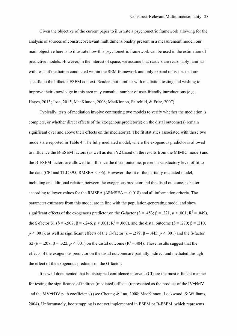
Construct-Relevant Multidimensionality 28
Given the objective of the current paper to illustrate a psychometric framework allowing for the
analysis of sources of construct-relevant multidimensionality present in a measurement model, our
main objective here is to illustrate how this psychometric framework can be used in the estimation of
predictive models. However, in the interest of space, we assume that readers are reasonably familiar
with tests of mediation conducted within the SEM framework and only expand on issues that are
specific to the bifactor-ESEM context. Readers not familiar with mediation testing and wishing to
improve their knowledge in this area may consult a number of user-friendly introductions (e.g.,
Hayes, 2013; Jose, 2013; MacKinnon, 2008; MacKinnon, Fairchild, & Fritz, 2007).
Typically, tests of mediation involve contrasting two models to verify whether the mediation is
complete, or whether direct effects of the exogenous predictor(s) on the distal outcome(s) remain
significant over and above their effects on the mediator(s). The fit statistics associated with these two
models are reported in Table 4. The fully mediated model, where the exogenous predictor is allowed
to influence the B-ESEM factors (as well as item Y2 based on the results from the MIMIC model) and
the B-ESEM factors are allowed to influence the distal outcome, present a satisfactory level of fit to
the data (CFI and TLI >.95; RMSEA < .06). However, the fit of the partially mediated model,
including an additional relation between the exogenous predictor and the distal outcome, is better
according to lower values for the RMSEA (ΔRMSEA = -0.018) and all information criteria. The
parameter estimates from this model are in line with the population-generating model and show
significant effects of the exogenous predictor on the G-factor (b = .453; β = .221, p < .001; R2 = .049),
the S-factor S1 (b = -.507; β = -.246, p < .001; R2 = .060), and the distal outcome (b = .270; β = .210,
p < .001), as well as significant effects of the G-factor (b = .279; β = .445, p < .001) and the S-factor
S2 (b = .207; β = .322, p < .001) on the distal outcome (R2 =.404). These results suggest that the
effects of the exogenous predictor on the distal outcome are partially indirect and mediated through
the effect of the exogenous predictor on the G-factor.
It is well documented that bootstrapped confidence intervals (CI) are the most efficient manner
for testing the significance of indirect (mediated) effects (represented as the product of the IVMV
and the MVDV path coefficients) (see Cheung & Lau, 2008; MacKinnon, Lockwood, & Williams,
2004). Unfortunately, bootstrapping is not yet implemented in ESEM or B-ESEM, which represents

Construct-Relevant Multidimensionality 29
another limitation of the way these models are currently implemented. However, these tests can easily
be implemented using the ESEM-Within-CFA (EWC) approach described by Morin, Marsh et al.
(2013; also see Marsh, Nagengast et al., 2013, as well as the input files provided here in the online
supplements). To implement this method, one needs to use the start values provided as part of the
final predictive ESEM or B-ESEM model, to add the constraints required for identification purposes,
and to re-estimate this model while requesting bootstraped estimation (see the online supplements for
details of implementation). When our final model is re-estimated using this method and requesting
bias-corrected bootstrapped confidence intervals, the results confirm that the indirect effect of the
exogenous predictor on the distal outcome, as mediated by the G-factor, is significant as indicated by
a bias-corrected bootstrapped 95% CI excluding 0 (indirect effect = b = .127; 95% CI = .088/.174).
Another limitation of current implementations is that all factors forming a single set of ESEM
or B-ESEM factors (i.e., a set of factors is defined as a group of factors defined by the same collection
of items allowed to have their main loadings or cross-loadings on all factors included in the group) are
required to be simultaneously related to other variables in the same manner (Asparouhov & Muthén,
2009; Marsh et al., 2009). Attempts to estimate a model where the factors forming a single set are
specified as having a different pattern of relations to other constructs (e.g., the exogenous predictor
predicts S1 and G, but not S2 and S3; or including a regression between S1 and the outcome, but a
correlation path between S2 and the outcome) would simply fail and produce a warning saying that
the model has been misspecified. In the present study, this means that the exogenous predictor needed
to be allowed to simultaneously predict the G-factor and the 3 S-factors. In turn, the G-factor and the
3 S-factors was simultaneously allowed to predict the distal outcome factor. Although this was not
necessary in the present application, the EWC method could have been used to circumvent this
limitation. To do so, one would simply need to use the start values from the final ESEM or B-ESEM
measurement model, to add the constraints required for identification purposes, and to replace the
factor correlations linking the ESEM/B-ESEM factors to the other variables by the required predictive
paths. We provide a sample input in the online supplements illustrating the implementation of this
method to estimate only the predictive paths depicted in Figure 2.
General Discussion

Construct-Relevant Multidimensionality 30
An Integrative Framework to Investigate Source of Construct-Relevant Multidimensionality
This study illustrated an overarching psychometric approach of broad relevance to
investigations of many complex multidimensional instruments routinely used in psychological and
educational research. More precisely, we showed how an integration of classical (CFA), emerging
(ESEM) and “rediscovered” (bifactor) models provides a general framework (bifactor-ESEM) for the
investigation of two sources construct-relevant psychometric multidimensionality related to (a) the
hierarchical nature of the constructs being assessed (i.e., the co-existence of global and specific
components within the same measurement model) and (b) the fallible nature of indicators which tend
to include at least some degree of association with non-target constructs. We argue that the first
source of construct-relevant multidimensionality naturally calls for bifactor models, while the second
source of construct-relevant multidimensionality rather calls for ESEM (rather than CFA). Thus,
when both sources of multidimensionality are present, then a bifactor-ESEM model should be
preferable. Such integrated models have only recently be made available and had yet to be
systematically applied to the investigation of complex measurement instruments.
The first step in the application of the proposed framework starts with a comparison of first-
order ICM-CFA and ESEM models to assess the presence of construct-relevant multidimensionality
due to the fallible nature of the indicators and reinforced by the presence of conceptually-related or
overlapping constructs. Given that bifactor models tend to absorb un-modeled cross-loadings through
the estimation of inflated global factors (Murray & Johnson, 2013), it is important that the application
of this framework always starts with a comparison of ESEM versus ICM-CFA models. In agreement
with previous recommendations (e.g., Marsh et al., 2014; Morin, Marsh et al., 2013), we argue that
this first comparison should routinely be conducted in the investigation of the measurement structure
of any multidimensional instrument. In the examples provided in this manuscript, ESEM solutions
provided a better fit to the data when compared to ICM-CFA models. The superiority of ESEM was
further corroborated by the observation of lower factor correlations, resulting in more clearly
differentiated factors. In line with previous recommendations (e.g., Morin, Marsh et al., 2013),
applied studies (e.g., Marsh et al., 2009, Marsh, Lüdtke et al., 2010; Morin & Maïano, 2011), and
simulations (Asparouhov & Muthén, 2009; Marsh, Lüdtke et al., 2013; Schmitt & Sass, 2011), these

Construct-Relevant Multidimensionality 31
observations converge in supporting the superiority of the ESEM solution – at least in the data sets
considered here. As previously reinforced, decisions regarding the appropriateness of alternative
models to represent sources of construct-relevant multidimensionality should not be taken in
disconnection from a detailed examination of parameter estimates and substantive theory. The ESEM
results from Study 1 showed that all factors were clearly defined by the expected pattern of target
loadings and non-target cross-loadings, with stronger cross-loadings between conceptually-related or
hierarchically-ordered scales. This last observation suggested the presence of construct-relevant
multidimensionality involving hierarchically-superior constructs.
The second step in the application of the proposed framework involves the comparison of
first-order versus bifactor and higher-order solutions (relying on ESEM or CFA depending on the
results from the first step), in order to assess the presence of construct-relevant multidimensionality
due to the presence of hierarchically-superior constructs. Although we argued that the first step of this
framework should be routinely applied to the investigation of any multidimensional instrument, this
second verification should only be conducted when substantive theory and the results from the first
step suggest that this second source of construct-relevant multidimensionality may be present in an
instrument. In the examples considered here, the bifactor-ESEM was retained as providing the best
fitting representation of the data after verification of theoretical (in Study 1) and empirical (in both
studies) conformity of the parameter estimates. Indeed, in the bifactor-ESEM solutions, the G-factors
were well-defined and clearly supported the presence of a global factor emerging from answers to the
full set of items. It is true that, in Study 1, the inclusion of items specifically designed to assess global
self-conceptions made the SDQ-I uniquely well suited to this illustration. However, the application of
bifactor models is in no way dependent on the presence of items directly tapping into a global
construct (e.g., Gignac & Watkins, 2013; Morin, Tran et al., 2013; Simms et al., 2008).
The Meaning of the Alternative Models
Construct-Relevant Multidimensionality: Items as Fallible Indicators of a Single
Construct. A common idea in applied research is that good indicators need to provide a perfect
reflection of a single construct, and that cross-loadings will inherently and irremediably change the
meaning of the constructs that are estimated. Rather, following Marsh et al. (2014), we argue here that

Construct-Relevant Multidimensionality 32
a completely pure item that has no cross-loadings or other sources of non-random specificity is a
convenient fiction – at best an impossible ideal and at worst a potentially serious distortion of reality
that undermines the valid interpretation of the data. Seeking such ideals, absolute truths, and other
golden rules in psychometrics that obviate subjective interpretations (Marsh et al., 2004) is not
inherently bad. However, applied researchers need to understand that pure items do not exist in reality
and will be rejected in a purely statistical sense when evaluated within a sufficiently broad framework
(with large Ns and a sufficiently large number of items and factors). Of course, misfit associated with
cross-loadings might be sufficiently trivial to be ignorable – providing an appropriate balance between
complexity and parsimony – but support for such claims should be based on empirical results.
The simple observation that many items are inherently expected to include construct-relevant
multidimensionality explaining their association with multiple constructs shows that this requirement
for pure indicators relies on a logic that inherently flawed. For example, in the assessment of anxiety
and depression (e.g., Gignac et al., 2007; Simms et al., 2008), cross-loadings are expected due to the
fact that some symptoms are inherently part of both disorders, such as insomnia and psychomotor
agitation. Our illustration based on the SDQ-I also provides interesting examples. For instance, “I
have a good looking body” (an indicator of physical appearance self-concept) had a significant non-
target cross-loading on physical ability self-concept, which could be related to the fact that athletic
bodies tend to be perceived as more attractive. Similar examples are numerous and show that cross-
loadings do not “taint” the constructs, but rather allow the constructs to be estimated using all of the
relevant information present at the indicator level. Remember that, according to the reflective logic of
factor analyses, the factors are specified as influencing the indicators, rather than the reverse. Thus,
small cross-loadings should be seen as reflecting the influence of the factor on the construct-relevant
part of the indicators, rather than the indicators having an impact on the nature of the factor itself. It
should be kept in mind that this interpretation applies to relatively small cross-loadings that are in line
with theoretical expectations, whereas any model showing large and unexplainable cross-loadings or
cross-loadings larger than target loadings should be re-examined.
Furthermore, factor correlations tend to be substantially biased when non-zero cross-loadings
are constrained to be zero (as shown in our simulated data set, as well as in Asparouhov & Muthén,

Construct-Relevant Multidimensionality 33
2009; Marsh, Lüdtke et al., 2013; Schmitt & Sass, 2011). This suggests that it is the exclusion of these
cross-loadings that can drastically change the meaning of the constructs. This clearly underlines the
importance for applied research to consider this additional source of construct-relevant psychometric
multidimensionality even when the initial ICM-CFA model appears to fit the data well (Marsh, Liem
et al., 2011; Marsh, Nagengast et al., 2011). As noted by Marsh et al. (2014, p. 104): “If the fit and
parameter estimates (e.g., latent factor correlations) for the ICM-CFA do not differ substantially from
the corresponding ESEM, on the basis of parsimony researchers should retain the CFA model”.
Alternatively, when the fit of the ESEM solution is acceptable, higher than the fit of the ICM-CFA,
and ESEM results in lower estimates of the factor correlations, then ESEM should be preferred.
It is true that rotational indeterminacy raises additional questions. Indeed, any ESEM solution
depends on the rotation procedure that is selected so that factors correlations and non-target cross-
loading can be directly increased or decreased by changing the rotation (Morin, & Maïano, 2011;
Schmitt & Sass, 2011). With this in mind, simulation studies still show that, notwithstanding this
issue, ESEM tends to provide factor correlation estimates that are closer to true population values,
even if they are themselves imperfect due to rotational indeterminacy (e.g., Asparouhov & Muthén,
2009; Marsh, Lüdtke et al., 2013; Schmitt & Sass, 2011). Furthermore, even when the true population
model corresponds to ICM-CFA, ESEM still tends to adequately recover true population values. In
this paper, we elected to rely on target rotation, which provides a confirmatory approach to ESEM
(see Marsh et al., 2014) and allows the analyst to specify the expected pattern of associations between
items and factors. Furthermore, when bifactor-ESEM models are specified as orthogonal (e.g., Chen
et al., 2006; Reise, 2012), these concerns are somehow diminished. However, the reader should keep
in mind that even for bifactor-ESEM, the selection of an orthogonal (versus oblique) rotation is itself
a choice and subject to rotational indeterminacy (see Endnote 1 and Jenrich & Bentler, 2012).
Construct-Relevant Multidimensionality: Hierarchically-Superior Constructs. Although
our main focus is on bifactor models as a method of choice to model construct-relevant
multidimensionality due to the presence of hierarchically-superior constructs, we also contrasted these
models with hierarchical models in t study 1. The SLP (described earlier) makes obvious that both
models estimate some form of global factor based on the covariance shared among all items, as well

Construct-Relevant Multidimensionality 34
as variance components reflecting specificity associated with groupings of items that remain
unexplained by the global factor (see also Chen et al., 2006). However, there are critical differences
between the two approaches. Statistically, the strict proportionality constraints that are at play in
hierarchical models limit their flexibility and practical applicability (Brunner et al., 2012; Chen et al.,
2006; Jenrich & Bentler, 2011; Reise, 2012). In line with this affirmation, the hierarchical-CFA and
hierarchical-ESEM systematically provided the worst fit to the data of all models estimated in the first
study. Substantively, the difference between these models is even more pronounced. A bifactor model
assumes the existence of an overarching construct underlying all indicators, and estimates the S-
factors from the part of the indicators that remains unexplained by this global component. The S-
factors are thus seen as conceptually distinct from the G-factor. Conversely, a hierarchical model
directly estimates the global factor from the first-order factors, rather than the indicators. The first-
order factors are thus a component of the global factor, rather than being separate from it.
As shown in our illustration based on simulated data, even when the true underlying
population model follows bifactor assumptions, it is possible for alternative first-order CFA or ESEM
models to provide a satisfactory level of fit to the data through the simple “absorption” of this
hierarchical structure via inflated factor correlations and/or item cross-loadings. However, these
alternative models are substantively erroneous in that they completely ignore the underlying global
construct that underlies responses to all indicators. In psychiatric measurement, Morin, Tran et al.
(2013, p. 2) note that “an important question has to do with whether a primary dimension (e.g.,
depression, anxiety, ADHD, etc.) does exist as a unitary disorder, including specificities (i.e., as
represented by a bifactor model), or whether these specificities rather define a set of distinct facets
without a generic common core (i.e., represented by a classical CFA model)”. Fortunately, a detailed
assessment of parameter estimates, theory, and statistical indices allowed us to pick the proper model
in this simulated data study, although the fit of the alternative models generally proved satisfactory
according to typical interpretation guidelines. Clearly, future simulation studies should investigate
more thoroughly the efficacy of the various goodness-of-fit indices and information criteria in
selecting the proper model amongst the alternative representations considered here.
Conclusion

Construct-Relevant Multidimensionality 35
This study was designed to illustrate an overarching psychometric framework for the
investigation of construct-relevant multidimensionality related to the fallible nature of the imperfect
indicators typically used in applied research, and to the assessment of hierarchically-superior
constructs within the same instrument. Although our results supported the use of bifactor-ESEM, we
do not claim that this specific psychometric representation will necessarily generalize to all
instruments that are routinely used in psychological, educational, and social sciences research.
However, we anticipate that this specific combination (i.e., bifactor-ESEM) may prove to be quite
important to consider when working with complex multidimensional measures. More generally, we
argue that the full framework proposed here should be routinely applied to studies of complex
instruments, especially those that include a separate subset of items specifically designed to assess
hierarchically-superior constructs. In these contexts, we believe that typical solutions of modeling
these items as a separate subscale, or simply of excluding them, should no longer be seen as adequate
as it ignores the inherently hierarchical nature of the assessed constructs.
Endnotes
1 Bifactor estimation relies on orthogonal factors to ensure interpretability of the results. However,
alternative models may be estimated where the S-factors are allowed to correlate to one another,
although these models often pose interpretation and/or convergence problems. In B-CFA (or CFA
more generally), orthogonal models are more parsimonious than comparative models based on
oblique factors, and thus provide a different fit to the data. However, in ESEM or B-ESEM, oblique or
orthogonal rotations have equivalent covariance implications and thus are statistically equivalent
models with identical fit to the data. To ensure comparability with typical bifactor applications, as
well as between B-CFA and B-ESEM, we relied on orthogonal rotation. However, exploring
alternative procedures confirmed that our main conclusions were unaffected by this choice.
2 An ESEM model including f factors is empirically impossible to distinguish from a B-ESEM model
including f-1 S-factors: Both are equivalent, have the same degrees of freedom, and produce the same
chi-square, fit indices, and information criteria (Hershberger & Marcoulides, 2013; MacCallum,
Wegener, Uchino, & Fabrigar, 1993). The reason for this is that in ESEM, each item is allowed to
load on all factors. So, in a B-ESEM model including f S-factors and one G-factor, each item is in fact

Construct-Relevant Multidimensionality 36
allowed to load on f +1 factors. This makes an ESEM model including f factors impossible to
distinguish from a B-ESEM model including f-1 S-factors as both, in the end, will estimate the
loadings of all items on a total of f factors. In fact, differences in results between these two solutions
can be attributed to the inherent rotational indeterminacy of any EFA/ESEM application (e.g., Morin
& Maïano, 2011; Morin, Marsh et al., 2013). For this reason, we recommend starting all comparisons
by contrasting an ESEM model including f factors with a B-ESEM model including the same number
of S-factors (i.e., only differing by the addition of the G-factor). Whenever the results from both
models provide an adequate and similar level of fit to the data, then the results from the B-ESEM
model should be systematically inspected in order to verify whether it makes sense to drop one of the
S-factor including items that should theoretically relate only to the G-factor.
References
Abu-Hilal, M.M., & Aal-Hussain, A.Q.A. (1997). Dimensionality and hierarchy of the SDQ in a non-
western milieu: A test of self-concept invariance across gender. Journal of Cross-Cultural
Psychology, 28, 535-553.
Akaike, H. (1987). Factor analysis and AIC. Psychometrika, 52, 317-332.
Arens, A.K., Yeung, A.S., Craven, R.G., & Hasselhorn, M. (2011). The twofold multidimensionality
of academic self-concept: Domain specificity and separation between competence and affect
components. Journal of Educational Psychology, 103, 970-981.
Arens, A.K., Yeung, A.S., Craven, R.G., & Hasselhorn, M. (2013). A short German version of the
Self-Description Questionnaire I: Theoretical and empirical comparability. International Journal
of Research & Method in Education, 36, 415-438.
Asparouhov, T. & Muthén, B.O. (2009). Exploratory structural equation modeling. Structural
Equation Modeling, 16, 397-438.
Barendse, M.T., Oort, F.J., & Garst, G.J. (2010). Using restricted factor analysis with latent
moderated structures to detect uniform and nonuniform measurement bias: A simulation study.
AStA-Advances in Statistical Analysis, 94, 117-127.
Barendse, M.T., Oort, F.J., Werner, C.S., Ligtvoet, R., & Schermelleh-Engel, K. (2012).
Measurement bias detection through factor analysis. Structural Equation Modeling, 19, 561-579.
Bentler, P. (1990). Comparative fit in structural models. Psychological Bulletin, 107, 238-246.

Construct-Relevant Multidimensionality 37
Bollen, K.A. (1989). Structural Equations with latent variables. New York, NY: Wiley.
Bozdogan, H. (1987). Model Selection and Akaike's information criterion (AIC): The general theory
and its analytical extensions. Psychometrika, 52, 345-370.
Browne, M.W. (2001). An overview of analytic rotation in exploratory factor analysis. Multivariate
Behavioral Research, 36, 111–150
Browne, M.W., & Cudeck, R. (1993). Alternative ways of assessing model fit. In K. A. Bollen, & J.
S. Long (Eds.), Testing structural equation models (pp. 136-162). Newbury Park, CA: Sage.
Brunner, M., Keller, U., Dierendonck, C., Reichert, M., Ugen, S., Fischbach, A., & Martin, R. (2010).
The structure of academic self-concepts revisited: The nested Marsh/Shavelson model. Journal of
Educational Psychology, 102, 964-981.
Brunner, M., Keller, U., Hornung, C., Reichert, M. & Martin, R. (2009). The cross-cultural
generalizability of a new structural model of academic self-concepts. Learning and Individual
Differences, 19, 387-403.
Brunner, M., Lüdtke, O., & Trautwein, U. (2008). The internal/external frame of reference model
revisited: Incorporating general cognitive ability and general academic self-concept. Multivariate
Behavioral Research, 43, 137-172.
Brunner, M., Nagy, G., & Wilhelm, O. (2012). A tutorial on hierarchically structured constructs.
Journal of Personality, 80, 796–846.
Byrne, B.M. (1996). Measuring self-concept across the life span: Issues and instrumentation.
Washington, DC: American Psychological Association.
Byrne, B.M., Shavelson, R.J., & Muthén, B.O. (1989). Testing for the equivalence of factor
structures: The issue of partial measurement invariance. Psychological Bulletin, 105, 456-466.
Caci, H., Morin, A.J.S., & Tran, A. (2013, in press). Teacher ratings of the ADHD-RS IV in a
community sample: Results from the ChiP-ARD study. Journal of Attention Disorders. Early
view, DOI: 10.1177/1087054712473834.
Chen, F.F. (2007). Sensitivity of goodness of fit indices to lack of measurement invariance. Structural
Equation Modeling, 14, 464-504.
Chen, F.F., West, S.G., & Sousa, K.H. (2006). A comparison of bifactor and second-order models of
quality of life. Multivariate Behavioral Research, 41, 189-255.
Cheung, G.W., & Lau, R.S. (2008). Testing mediation and suppression effects of latent variables:

Construct-Relevant Multidimensionality 38
Bootstrapping with structural equation models. Organizational Research Methods, 11, 296-325.
Cheung, G.W., & Lau, R.S. (2012). A direct comparison approach for testing measurement
invariance. Organizational Research Methods, 15, 167-198.
Cheung, G.W. & Rensvold, R.B. (2002). Evaluating goodness-of-fit indexes for testing measurement
invariance. Structural Equation Modeling, 9, 233-255.
Eid, M., Nussbeck, F.W., Geiser, C., Cole, D.A., Gollwitzer, M., & Lischetzke, M (2008). Structural
equation modelling of multitrait-multimethod data: Different models for different types of
methods. Psychological Methods, 13, 230-253.
Enders, C.K. (2010). Applied missing data analysis. New York: Guilford.
Fan, X., & Sivo, S.A. (2005). Sensitivity of fit indexes to misspecified model components: Rationale
of two-index strategy revisited. Structural Equation Modeling, 12, 343-367.
Fan, X., & Sivo, S.A. (2007). Sensitivity of fit indices to model misspecification and model types.
Multivariate Behavioral Research, 42, 509-529
Fan, X., & Sivo, S.A. (2009). Using goodness-of-fit indexes in assessing mean structure invariance.
Structural Equation Modeling, 16, 54-69.
Gignac, G.E. (2007). Multi-factor modeling in individual differences research: Some
recommendations and suggestions. Personality and Individual Differences, 42, 37-48.
Gignac, G.E., Palmer, B., & Stough, C. (2007). A confirmatory factor analytic investigation of the
TAS-20: Corroboration of a five-factor model and suggestions for improvement. Journal of
Personality Assessment, 89, 247-257.
Gignac, G.E., & Watkins, M.W. (2013). Bifactor modeling and the estimation of model-based
reliability in the WAIS-IV. Multivariate Behavioral Research, 48, 639-662.
Graham, J.W. (2009). Missing data analysis: Making it work in the real world. Annual Review of
Psychology, 60, 549-576.
Grimm, K. J., Steele, J. S., Ram, N., & Nesselroade, J. R. (2013). Exploratory latent growth models in
the structural equation modeling framework. Structural Equation Modeling, 20, 568-591.
Hayes, A. F. (2013). Introduction to mediation, moderation, and conditional process analysis: A
regression-based approach. New York: Guilford.
Hershberger, S.L., & Marcoulides, G.A. (2013). The problem of equivalent structural models. In
Hancock, G.R., & Mueller, R.O. (Eds.). Structural equation modeling: A second course (2nd ed.,

Construct-Relevant Multidimensionality 39
pp. 13-42). Charlotte, NC: Information Age Publishing, Inc.
Hu, L.-T., & Bentler, P.M. (1998). Fit indices in covariance structure modeling: Sensitivity to
underparameterized model misspecification. Psychological Methods, 3, 424-453.
Holzinger, K.J., & Swineford, F. (1937). The bi-factor model. Psychometrika, 2, 1-17.
Jennrich, R.I., & Bentler, P.M. (2011). Exploratory bi-factor analysis. Psychometrika, 76, 537– 549.
Jennrich, R.I., & Bentler, P.M. (2012). Exploratory bi-factor analysis: The oblique case.
Psychometrika, 77, 442-454.
Jöreskog, K.G. (1973). A general method for estimating a linear structural equation system. In A.S.
Golberger, & O.D. Duncan (Eds.), Structural equation models in the social sciences (pp. 85-112).
New York, NY: Seminar.
Jöreskog, K.G., & Goldberger, A. (1975). Estimation of a model with multiple indicators and multiple
causes of a single latent variable. Journal of the American Statistical Association, 10, 631-639.
Jose, P.E. (2013). Doing statistical mediation and moderation. New York: Guilford.
MacCallum, R.C., Wegener, D.T., Uchino, B.N., & Fabrigar, L.R. (1993). The problem of equivalent
models in applications of covariance structure analysis. Psychological Bulletin, 114, 185-199.
MacKinnon, D.P. (2008). Introduction to statistical mediation analysis. Mahwah, NJ: Erlbaum.
MacKinnon, D.P., Fairchild, A.J., & Fritz, M.S. (2007). Mediation analysis. Annual Review of
Psychology, 58, 593 -614.
MacKinnon, D.P., Lockwood, C.M., & Williams, J. (2004). Confidence limits for the indirect effect:
Distribution of product and resampling methods. Multivariate Behavioral Research, 39, 99-128.
Marsh, H.W. (1987). The hierarchical structure of self-concept and the application of hierarchical
confirmatory factor analyses. Journal of Educational Measurement, 24, 17-39.
Marsh, H.W. (1989). Age and sex effects in multiple dimensions of self-concept: Preadolescence to
early adulthood. Journal of Educational Psychology, 82, 417-430.
Marsh, H.W. (1990). Self-Description Questionnaire – I (SDQ-I). Manual. Macarthur, N.S.W.
Australia: University of Western Sydney.
Marsh, H.W. (2007). Self-concept theory, measurement and research into practice: The role of self-
concept in educational psychology. Leicester, UK: British Psychological Society.
Marsh, H.W., Abduljabbar, A.S., Abu-Hilal, M., Morin, A.J.S., Abdelfattah, F., Leung, K.C., Xu,
M.K., Nagengast, B., & Parker, P. (2013). Factor structure, discriminant and convergent validity

Construct-Relevant Multidimensionality 40
of TIMSS math and science motivation measures: A comparison of USA and Saudi Arabia.
Journal of Educational Psychology, 105, 108-128.
Marsh, H.W., & Ayotte, V. (2003). Do multiple dimensions of self-concept become more
differentiated with age? The differential distinctiveness hypothesis. Journal of Educational
Psychology, 95, 687-706.
Marsh, H.W., Hau, K.-T., & Grayson, D. (2005). Goodness of fit evaluation in structural equation
modeling. In A. Maydeu-Olivares & J. McArdle (Eds.), Contemporary psychometrics. A
Festschrift for Roderick P. McDonald. Mahwah NJ: Erlbaum.
Marsh, H.W., Hau, K.-T., & Wen, Z. (2004). In search of golden rules: Comment on hypothesis-
testing approaches to cutoff values for fit indexes and dangers in overgeneralizing Hu & Bentler’s
(1999). Structural Equation Modeling, 11, 320-341.
Marsh, H.W., & Hocevar, D. (1985). Application of confirmatory factor analysis to the study of self-
concept: First- and higher order factor models and their invariance across grades. Psychological
Bulletin, 97, 562-582.
Marsh, H.W., Liem, G.A.D., Martin, A.J., Morin, A.J.S., & Nagengast, B. (2011). Methodological
measurement fruitfulness of exploratory structural equation model: New approaches to issues in
motivation and engagement. Journal of Psychoeducational Assessment, 29, 322-346.
Marsh, H.W., Lüdtke, O., Muthén, B., Asparouhov, T., Morin, A. J. S., Trautwein, U., & Nagengast,
B. (2010). A new look at the big-five factor structure through exploratory structural equation
modeling. Psychological Assessment, 22, 471-491.
Marsh, H.W., Lüdtke, O., Nagengast, B., Morin, A.J.S., & Von Davier, M. (2013). Why item parcels
are (almost) never appropriate: Two wrongs do not make a right—Camouflaging misspecification
with item parcels in CFA models. Psychological Methods, 18, 257-284.
Marsh, H.W., Morin, A.J.S., Parker, P.D., & Kaur, G. (2014). Exploratory structural equation
modelling: An integration of the best features of exploratory and confirmatory factor analyses.
Annual Review of Clinical Psychology, 10, 85-110.
Marsh, H.W., Muthén, B., Asparouhov, A., Lüdtke, O., Robitzsch, A., Morin, A.J.S., & Trautwein, U.
(2009). Exploratory structural equation modeling, integrating CFA and EFA: Application to
students' evaluations of university teaching. Structural Equation Modeling, 16, 439-476.
Marsh, H.W., Nagengast, B., & Morin, A.J.S. (2013). Measurement invariance of big-five factors

Construct-Relevant Multidimensionality 41
over the life span: ESEM tests of gender, age, plasticity, maturity, and La Dolce Vita effects.
Developmental Psychology, 49, 1194-1218.
Marsh, H.W., Nagengast, B., Morin, A.J.S., Parada, R.H., Craven, R.G., & Hamilton, L.R. (2011).
Construct validity of the multidimensional structure of bullying and victimization: An application
of exploratory structural equation modeling. Journal of Educational Psychology, 103, 701-732.
Marsh, H.W., Scalas, L.F., & Nagengast, B. (2010). Longitudinal tests of competing G-factor
structures for the Rosenberg self-esteem scale: Traits, ephemeral artifacts, and stable response
styles. Psychological Assessment, 22, 366-381.
Marsh, H.W., Tracey, D.K., & Craven, R.G. (2006). Multidimensional self-concept structure for
preadolescents with mild intellectual disabilities: A hybrid multigroup-mimic approach.
Educational and Psychological Measurement, 66, 795-818.
McCrae, R.R., Zonderman, A.B., Costa, P.T.Jr., Bond, M.H., & Paunonen, S. (1996). Evaluating the
replicability of factors in the revised NEO Personality Inventory: Confirmatory factor analysis
versus Procrustes rotation. Journal of Personality and Social Psychology, 70, 552–566.
Meleddu, M., Guicciardi, M., Scalas, L.F., & Fadda, D. (2012). Validation of an Italian version of the
Oxford Happiness Inventory in adolescence. Journal of Personality Assessment, 94, 175-185.
Meredith, W. (1993). Measurement invariance, factor analysis and factorial invariance.
Psychometrika, 58, 525-543.
Millsap, R.E. (2011). Statistical approaches to measurement invariance. New York: Routledge.
Möller, J., Pohlmann, B., Köller, O., & Marsh, H. W. (2009). Meta-analytic path analysis of the
internal/external frame of reference model of academic achievement and academic self-concept.
Review of Educational Research, 79, 1129-1167.
Morin, A. J. S., & Maïano, C. (2011). Cross-validation of the short form of the physical self-inventory
(PSI-S) using exploratory structural equation modeling (ESEM). Psychology of Sport & Exercise,
12, 540-554.
Morin, A. J. S., Marsh, H. W., & Nagengast, B. (2013). Exploratory structural equation modeling. In
Hancock, G. R., & Mueller, R. O. (Eds.). Structural equation modeling: A second course (2nd ed.,
pp. 395-436). Charlotte, NC: Information Age Publishing, Inc.
Morin, A.J.S., Tran, A., & Caci, H. (2013, in press). Factorial validity of the ADHD Adult Symptom
Rating Scale in a French community sample. Journal of Attention Disorders. Early view, DOI:

Construct-Relevant Multidimensionality 42
10.1177/1087054713488825
Murray, A.L., & Johnson, W. (2013). The limitations of model fit in comparing the bi-factor versus
higher-order models of human cognitive ability structure. Intelligence, 41, 407-422.
Muthén, B.O. (1989). Latent variables in heterogenous populations. Psychometrika, 54, 557-585.
Muthén, L.K., & Muthén, B.O. (1998 –2012). Mplus user’s guide. Seventh edition. Los Angeles, CA:
Muthén & Muthén.
Reise, S.P. (2012). The rediscovery of bifactor measurement models. Multivariate Behavioral
Research, 47, 667–696.
Reise, S.P., Moore, T.M., & Haviland, M.G. (2010). Bifactor models and rotations: Exploring the
extent to which multidimensional data yield univocal scale scores. Journal of Personality
Assessment, 92, 544-559.
Reise, S.P., Moore, T.M., & Maydeu-Olivares, A. (2011). Targeted bifactor rotations and assessing
the impact of model violations on the parameters of unidimensional and bifactor models.
Educational and Psychological Measurement, 71, 684–711.
Reise, S.P., Morizot, J., & Hays, R.D. (2007). The role of the bifactor model in resolving
dimensionality issues in health outcomes measures. Quality of Life Research, 16, 19-31.
Rindskopf, D., & Rose, T. (1988). Some theory and applications of confirmatory second-order factor
analyses. Multivariate Behavioral Research, 23, 51-67.
Schmid, J., & Leiman, J.M. (1957). The development of hierarchical factor solutions. Psychometrika,
22, 53–61.
Schmitt, T.A., & Sass, D.A. (2011). Rotation criteria and hypothesis testing for exploratory factor
analysis: implications for factor pattern loadings and interfactor correlations. Educational &
Psychological Measurement, 71, 95-113.
Schwartz, G. (1978). Estimating the dimension of a model. The Annals of Statistics, 6, 461-464.
Schweizer, K. (2012). On correlated errors. European Journal of Psychological Assessment, 28, 1-2.
Sclove, L. (1987). Application of model-selection criteria to some problems in multivariate analysis.
Psychometrika, 52, 333-343.
Shavelson, R.J., Hubner, J.J. & Stanton, G.C. (1976). Self-concept: Validation of construct
interpretations. Journal of Educational Research, 46, 407-441.
Simms, L.J., Grös, D.F., Watson, D., & O’Hara, M. (2008). Parsing general and specific components

Construct-Relevant Multidimensionality 43
of depression and anxiety with bifactor modeling. Depression and Anxiety, 25, 34–46.
Steiger, J. H. (1990). Structural model evaluation and modification: An interval estimation approach.
Multivariate Behavioral Research, 25, 173-180.
Tucker, L. R., & Lewis, C. (1973). A reliability coefficient for maximum likelihood factor analysis.
Psychometrika, 38, 1–10.
Vispoel, W.P. (1995). Self-concept in artistic domains: An extension of the Shavelson, Hubner, and
Stanton (1976) model. Journal of Educational Psychology, 87, 134-153
Watkins, D., & Akande, A. (1992). Internal structure of the Self-Description Questionnaire: A
Nigerian investigation. British Journal of Educational Psychology, 62, 120-125.
Watkins, D., & Dong, Q. (1994). Assessing the self-esteem of Chinese school children. Educational
Psychology, 14, 129-137.
Watkins, D., Juhasz, A.M., Walker, A., & Janvlaitiene, N. (1995). The Self-Description
Questionnaire-1: Lithuanian. European Journal of Psychological Assessment, 11, 41-51.
Yung, Y.F., Thissen, D., & McLeod, L.D. (1999). On the relationship between the higher-order factor
model and the hierarchical factor model. Psychometrika, 64, 113–128.

Construct-Relevant Multidimensionality 44
F1
X1
X2
X3
Y1
Y2
Y3
Z1
Z2
Z3
F2 F3
ESEM
F1
X1
X2
X3
Y1
Y2
Y3
Z1
Z2
Z3
F2 F3
ICM-CFA
F1
X1
X2
X3
Y1
Y2
Y3
Z1
Z2
Z3
F2 F3
HF
Hierarchical-CFA
F1
X1
X2
X3
Y1
Y2
Y3
Z1
Z2
Z3
F2 F3
Hierarchical-ESEM
HF
S1
X1
X2
X3
Y1
Y2
Y3
Z1
Z2
Z3
S2 S3
Bifactor-CFA
G
S1
X1
X2
X3
Y1
Y2
Y3
Z1
Z2
Z3
S2 S3
Bifactor-ESEM
G
Figure 1. Graphical representation of the alternative models considered in this study. Note. CFA= Confirmatory factor analyses; ICM = Independent cluster model; ESEM = Exploratory structural equation modeling; X1-X3, Y1-Y3, Z1-Z3 = Items; F1-F3: Factors; HF: Higher-order factors; S1-S3: Specific factors in a bifactor model; G = Global factor in a bifactor model; Ovals represent latent factors and squares represent observed variables; full unidirectional arrows linking ovals and squares represent the main factor loadings; dotted unidirectional arrows linking ovals and squares represent the cross-loadings; full unidirectional arrows linked to the items or the factors represent the item uniquenesses or factor disturbances; bidirectional full arrows linking the ovals represent factor covariances/correlations; bidirectional dashed arrows connecting a single oval represent factor variances.
X1 X2 X3 X4 Y1 Y2 Y3 Y4 Z1 Z2 Z3 Z4 W1 W2 W3 W4
Group
S1 S2 S3
O
G
b = .5
b = .5
b = .3
b = .5
b = .5 b = -.5
Figure 2. Graphical representation of the population generating model. Note. Circles represent latent factors and squares represent observed variables; dotted unidirectional arrows linking ovals and squares represent the factor loadings and cross loadings; full unidirectional arrows the ovals and squares represent regressions; full unidirectional arrows placed under the squares represent the item uniquenesses; full unidirectional arrows placed under the circles the factor disturbances; bidirectional dashed arrows connecting a single oval represent factor variances.
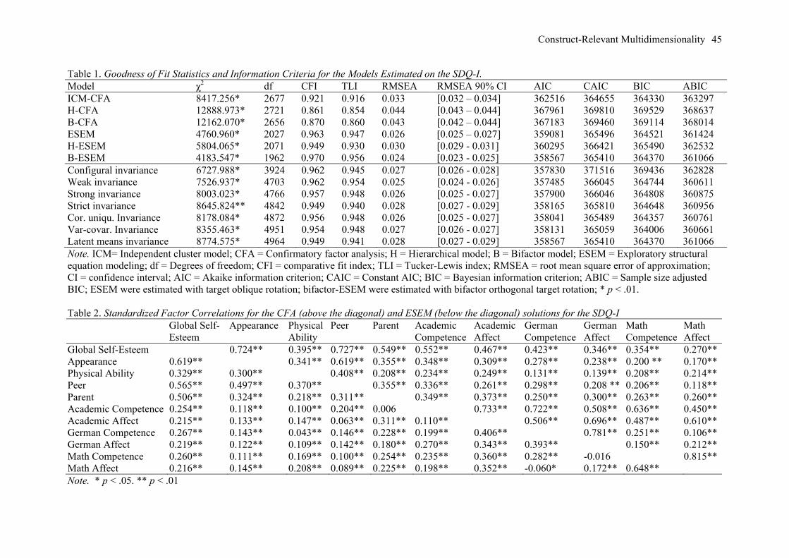
Construct-Relevant Multidimensionality 45
Table 1. Goodness of Fit Statistics and Information Criteria for the Models Estimated on the SDQ-I. Model χ2 df CFI TLI RMSEA RMSEA 90% CI AIC CAIC BIC ABIC ICM-CFA 8417.256* 2677 0.921 0.916 0.033 [0.032 – 0.034] 362516 364655 364330 363297 H-CFA 12888.973* 2721 0.861 0.854 0.044 [0.043 – 0.044] 367961 369810 369529 368637 B-CFA 12162.070* 2656 0.870 0.860 0.043 [0.042 – 0.044] 367183 369460 369114 368014 ESEM 4760.960* 2027 0.963 0.947 0.026 [0.025 – 0.027] 359081 365496 364521 361424 H-ESEM 5804.065* 2071 0.949 0.930 0.030 [0.029 - 0.031] 360295 366421 365490 362532 B-ESEM 4183.547* 1962 0.970 0.956 0.024 [0.023 - 0.025] 358567 365410 364370 361066 Configural invariance 6727.988* 3924 0.962 0.945 0.027 [0.026 - 0.028] 357830 371516 369436 362828 Weak invariance 7526.937* 4703 0.962 0.954 0.025 [0.024 - 0.026] 357485 366045 364744 360611 Strong invariance 8003.023* 4766 0.957 0.948 0.026 [0.025 - 0.027] 357900 366046 364808 360875 Strict invariance 8645.824** 4842 0.949 0.940 0.028 [0.027 - 0.029] 358165 365810 364648 360956 Cor. uniqu. Invariance 8178.084* 4872 0.956 0.948 0.026 [0.025 - 0.027] 358041 365489 364357 360761 Var-covar. Invariance 8355.463* 4951 0.954 0.948 0.027 [0.026 - 0.027] 358131 365059 364006 360661 Latent means invariance 8774.575* 4964 0.949 0.941 0.028 [0.027 - 0.029] 358567 365410 364370 361066 Note. ICM= Independent cluster model; CFA = Confirmatory factor analysis; H = Hierarchical model; B = Bifactor model; ESEM = Exploratory structural equation modeling; df = Degrees of freedom; CFI = comparative fit index; TLI = Tucker-Lewis index; RMSEA = root mean square error of approximation; CI = confidence interval; AIC = Akaike information criterion; CAIC = Constant AIC; BIC = Bayesian information criterion; ABIC = Sample size adjusted BIC; ESEM were estimated with target oblique rotation; bifactor-ESEM were estimated with bifactor orthogonal target rotation; * p < .01. Table 2. Standardized Factor Correlations for the CFA (above the diagonal) and ESEM (below the diagonal) solutions for the SDQ-I Global Self-
Esteem Appearance Physical
Ability Peer Parent Academic
Competence Academic Affect
German Competence
German Affect
Math Competence
Math Affect
Global Self-Esteem 0.724** 0.395** 0.727** 0.549** 0.552** 0.467** 0.423** 0.346** 0.354** 0.270** Appearance 0.619** 0.341** 0.619** 0.355** 0.348** 0.309** 0.278** 0.238** 0.200 ** 0.170** Physical Ability 0.329** 0.300** 0.408** 0.208** 0.234** 0.249** 0.131** 0.139** 0.208** 0.214** Peer 0.565** 0.497** 0.370** 0.355** 0.336** 0.261** 0.298** 0.208 ** 0.206** 0.118** Parent 0.506** 0.324** 0.218** 0.311** 0.349** 0.373** 0.250** 0.300** 0.263** 0.260** Academic Competence 0.254** 0.118** 0.100** 0.204** 0.006 0.733** 0.722** 0.508** 0.636** 0.450** Academic Affect 0.215** 0.133** 0.147** 0.063** 0.311** 0.110** 0.506** 0.696** 0.487** 0.610** German Competence 0.267** 0.143** 0.043** 0.146** 0.228** 0.199** 0.406** 0.781** 0.251** 0.106** German Affect 0.219** 0.122** 0.109** 0.142** 0.180** 0.270** 0.343** 0.393** 0.150** 0.212** Math Competence 0.260** 0.111** 0.169** 0.100** 0.254** 0.235** 0.360** 0.282** -0.016 0.815** Math Affect 0.216** 0.145** 0.208** 0.089** 0.225** 0.198** 0.352** -0.060* 0.172** 0.648** Note. * p < .05. ** p < .01

Construct-Relevant Multidimensionality 46
Table 3 Standardized Factor Loadings for Bifactor-ESEM Solution of the SDQ-I Items Global Self
Esteem Appearance Physical
Ability Peer Parent Academic
Competence Academic Affect
German Competence
German Affect
Math Competence
Math Affect G-Factor Uniquenesses
29 0.101 0.052* 0.053* 0.062* 0.000 -0.027 0.023 -0.067* 0.099** -0.090** -0.014 0.451** 0.753** 37 0.277** 0.216** -0.013 0.119** 0.160** -0.033 0.042 0.026 -0.104** 0.030 -0.040 0.320** 0.637** 45 0.381** 0.294** 0.088** 0.031 0.202** -0.141** 0.083 -0.047 -0.018 0.022 0.012 0.389** 0.538** 53 0.348** 0.082** 0.072** 0.131** 0.173** -0.049 0.002 -0.035 -0.029 -0.032 -0.035 0.519** 0.544** 61 0.273** 0.053* -0.038 0.056* 0.198** 0.008 -0.010 0.128** -0.125** 0.022 -0.077 0.433** 0.519** 67 0.306** 0.025 0.027 0.110** 0.012 0.070 -0.118** -0.056* -0.069** 0.013 -0.065** 0.610** 0.489** 70 0.280** 0.100** -0.023 0.254** 0.034 0.056 -0.061 -0.077* -0.025 -0.146** -0.022 0.469** 0.590** 72 0.411** 0.281** 0.036 0.098** -0.003 -0.017 -0.083** -0.089** -0.076** -0.121** -0.045* 0.557** 0.393** 74 0.355** 0.072** 0.002 0.086** -0.037 0.073 -0.132** -0.010 -0.046 -0.008 -0.118** 0.566** 0.500** 76 0.368** 0.048* 0.025 0.051* 0.028 -0.024 -0.064* -0.077** -0.047* -0.025 -0.087** 0.594** 0.484** 1 0.072** 0.629** 0.056** 0.094** -0.004 -0.015 -0.007 -0.017 -0.060** -0.045* -0.013 0.379** 0.438** 8 0.175** 0.589** 0.102** 0.083** 0.074** -0.086 0.060 -0.010 -0.026 0.005 0.029 0.392** 0.433** 15 0.021 0.690** 0.001 0.092** 0.003 -0.005 -0.005 -0.004 0.004 -0.058* -0.064** 0.449** 0.305** 22 0.030 0.724** -0.020** 0.077** 0.011 0.026 -0.015 -0.046* -0.021 -0.056** -0.069** 0.478** 0.229** 30 0.240** 0.528** 0.030 0.054* 0.128** -0.080 0.023 0.002 -0.038 0.035 0.010 0.376** 0.452** 38 -0.010 0.378** 0.050* 0.281** -0.058* 0.116* -0.117** -0.086* -0.038 -0.126** -0.062* 0.428** 0.533** 46 0.097* 0.307** 0.219** 0.050 0.017 -0.100* -0.016 -0.010 -0.066* -0.054* -0.055* 0.484** 0.590** 54 0.009 0.365** 0.054* 0.099** -0.099** 0.086 -0.219** -0.169** -0.099** -0.069** -0.134** 0.400** 0.567** 62 0.216** 0.350** -0.011 0.074** 0.029 0.038 -0.111** -0.038 -0.013 -0.119** -0.032 0.441** 0.599** 3 -0.068 0.085** 0.619** 0.065** -0.054* -0.213** -0.058 0.018 -0.069 -0.047 -0.022 0.348** 0.420** 10 0.025 0.010 0.512** 0.030 0.067** -0.138** 0.098* -0.013 0.030 -0.002 0.019 0.221** 0.653** 17 0.119** 0.024 0.744** 0.095** 0.068** 0.342** 0.127 0.009 0.011 0.044 0.052 0.118** 0.267** 24 0.090* 0.024 0.783** 0.095** 0.047* 0.264** 0.097 -0.023 0.055 0.016 0.047 0.180** 0.249** 32 -0.005 0.073** 0.351** 0.055 -0.068** -0.062 -0.164** -0.184** -0.014 -0.025 -0.002 0.300** 0.708** 40 0.010 0.045** 0.809** 0.059** -0.008 -0.058 -0.030 -0.020 -0.057** -0.012 0.003 0.320** 0.229** 48 -0.049 -0.026 0.575** 0.025 -0.021 -0.123** -0.106** -0.046 -0.050 -0.004 0.002 0.403** 0.472** 56 -0.020 0.050** 0.786** 0.037 -0.043** -0.117** -0.064 -0.037 -0.063* -0.062** -0.029 0.399** 0.189** 64 -0.039 0.041 0.487** 0.048 -0.012 -0.100* -0.067 -0.150** -0.059* 0.037 0.038 0.320** 0.612** 7 0.085* 0.070** 0.127** 0.589** 0.116** -0.117 0.120** 0.056* -0.011 0.032 -0.051* 0.242** 0.518** 14 0.009 0.051* 0.056** 0.518** -0.031 -0.045 0.008 0.047* -0.025 -0.011 -0.089** 0.317** 0.611** 21 0.028 0.055** 0.101** 0.575** 0.042 0.010 0.010 0.086** -0.073** 0.023 -0.108** 0.271** 0.523** 28 0.071 0.043 0.117** 0.504** 0.113** -0.112* 0.082* 0.019 -0.016 -0.017 -0.012 0.364** 0.560** 36 0.128** 0.232** 0.019 0.333** -0.004 -0.012 -0.027 -0.034 -0.075** -0.059* -0.048* 0.398** 0.647** 44 0.074 0.147** 0.025 0.499** 0.004 0.054 -0.107** -0.083** -0.021 -0.097** -0.042 0.448** 0.490** 52 0.016 0.085** 0.055** 0.458** -0.044* 0.041 -0.135** -0.133** -0.018 -0.027 -0.058* 0.370** 0.599** 60 0.073 0.112** 0.060** 0.454** -0.048* 0.088 -0.236** -0.098** -0.093** -0.060* -0.090** 0.486** 0.441** 69 0.156** 0.143** 0.076** 0.546** -0.007 0.053 -0.123** -0.095** -0.051* -0.118** -0.060** 0.497** 0.357**

Construct-Relevant Multidimensionality 47
Items Global Self Esteem
Appearance Physical Ability
Peer Parent Academic Competence
Academic Affect
German Competence
German Affect
Math Competence
Math Affect G-Factor Uniquenesses
5 0.086** 0.027 0.024 0.022 0.542** -0.028 0.038 0.002 0.038 -0.005 0.012 0.387** 0.543** 12 0.103** -0.004 -0.058* 0.022 0.313** 0.068 0.017 0.107** -0.053 0.095** -0.032 0.311** 0.666** 19 0.086 0.047** 0.028 -0.003 0.558** -0.073 0.032 -0.014 0.053* -0.005 0.016 0.281** 0.589** 26 0.096* 0.088** 0.013 0.042 0.535** -0.011 -0.018 0.009 0.032 0.017 -0.012 0.302** 0.601** 34 0.006 -0.002 -0.004 0.052* 0.413** 0.046 0.019 -0.017 0.001 -0.040 -0.019 0.347** 0.702** 42 -0.005 -0.013 0.014 0.056 0.503** 0.089 -0.055 -0.090* -0.004 -0.047 -0.031 0.430** 0.537** 50 0.021 -0.002 -0.018 -0.017 0.699** -0.042 -0.008 -0.050* 0.029 0.016 0.028 0.414** 0.332** 58 0.059* 0.020 -0.028 -0.012 0.758** -0.060** 0.017 -0.050* -0.014 -0.021 0.004 0.423** 0.235** 66 0.024 -0.024 0.029 0.032 0.650** 0.040 -0.079* -0.078** -0.053** -0.090** 0.019 0.432** 0.363** 2 -0.102** -0.044** -0.074** -0.100** -0.068** 0.099 0.199** 0.267** -0.152** 0.155** -0.074** 0.604** 0.429** 16 -0.128 -0.080** -0.065** -0.083** -0.043* 0.089 0.201** 0.293** -0.168** 0.142** -0.074** 0.638** 0.369** 31 -0.067* -0.131** -0.046* -0.091* -0.060** 0.083 0.095** 0.170** -0.053* 0.168** -0.055** 0.628** 0.491** 47 0.118** -0.017 -0.014 -0.025 0.061* -0.011 -0.001 0.220** 0.013 0.131** -0.025 0.446** 0.550** 63 -0.070* -0.122** -0.076** -0.112** -0.101** 0.070 0.208** 0.099** -0.075** 0.154** -0.042 0.691** 0.386** 9 -0.071** -0.011 -0.038* -0.094** 0.035 -0.024 0.367** -0.021 0.126** -0.065** 0.134** 0.585** 0.467** 23 0.062 -0.011 -0.008 -0.020 0.092** 0.061 0.174** 0.085** 0.188** 0.007 0.180** 0.372** 0.624** 39 -0.087** -0.097** -0.014 -0.128** -0.058 0.067 0.406** -0.087** 0.179** -0.049 0.147** 0.632** 0.331** 55 -0.075** -0.097** -0.027 -0.096** -0.037* 0.021 0.404** -0.102** 0.232** -0.065** 0.195** 0.644** 0.289** 71 -0.083** -0.131** -0.021 -0.111** -0.050** 0.051 0.418** -0.097** 0.196** 0.022 0.163** 0.658** 0.276** 4 -0.060** -0.041* -0.117** -0.052** -0.054** 0.050 -0.029 0.596** 0.106** -0.054* -0.132** 0.530** 0.303** 18 -0.081 -0.061** -0.086** -0.021 -0.055** 0.014 -0.028 0.595** 0.260** -0.023 -0.151** 0.548** 0.233** 33 0.016 -0.023 -0.066** -0.044** -0.006 0.047 -0.039 0.524** 0.235** -0.004 -0.084** 0.508** 0.364** 49 -0.036 -0.091** -0.087** -0.021 -0.064** 0.005 -0.069** 0.490** 0.336** -0.035 -0.145** 0.530** 0.317** 73 -0.007 -0.113** -0.043* -0.036 -0.102** 0.014 -0.049 0.388** 0.291** -0.024 -0.187** 0.597** 0.343** 11 -0.063** -0.004 -0.068** -0.054** 0.001 -0.032 0.122** 0.284** 0.595** -0.122** -0.047** 0.461** 0.309** 25 -0.070** -0.026 -0.043* -0.055** 0.017 -0.018 0.120** 0.159** 0.618** -0.090** -0.008 0.486** 0.322** 41 -0.071** -0.069** -0.008 -0.045** 0.004 -0.009 0.103** 0.160** 0.635** -0.124** -0.030 0.515** 0.268** 57 -0.066 -0.073** -0.049** -0.076** 0.003 -0.021 0.118** 0.175** 0.651** -0.122** -0.014 0.541** 0.206** 65 -0.003 -0.087 -0.051** -0.065** 0.009 0.016 0.071** 0.233** 0.566** -0.083** -0.040* 0.454** 0.333** 13 -0.051* -0.069** -0.018 -0.034* -0.041* 0.000 -0.016 -0.071** -0.115** 0.616** 0.336** 0.423** 0.300** 27 -0.058** -0.054** -0.045** -0.055** -0.028 0.029 0.004 0.036 -0.134** 0.622** 0.230** 0.491** 0.287** 43 -0.028 -0.096** 0.015 -0.027 -0.019 -0.010 -0.034 -0.048* -0.102** 0.557** 0.344** 0.543** 0.251** 59 -0.036* -0.072** -0.017 -0.070** -0.036* 0.016 -0.025 -0.027 -0.098** 0.630** 0.347** 0.542** 0.164** 75 0.018 -0.073** 0.009 -0.067** 0.015 0.049 -0.030 -0.016 -0.108** 0.572** 0.315** 0.457** 0.309** 6 -0.036 -0.043** 0.016 -0.084** 0.041* -0.013 0.048** -0.079** -0.078** 0.298* 0.644** 0.333** 0.347** 20 -0.047** -0.046** -0.005 -0.094 0.011 0.005 0.113** -0.113** -0.009 0.253** 0.690** 0.454** 0.215** 35 -0.071** -0.045** 0.026 -0.071** -0.005 0.003 0.090** -0.118** 0.001 0.265** 0.690** 0.464** 0.204** 51 -0.026 -0.043** 0.025 -0.098** -0.016** 0.011 0.076** -0.099** -0.037** 0.275** 0.763** 0.460** 0.100** 68 -0.060** -0.086** 0.039** -0.062** -0.013 -0.040* 0.095** -0.109** 0.000 0.282** 0.657** 0.478** 0.221**
Note. Negatively worded items are italicized; * p < .05. ** p < .01
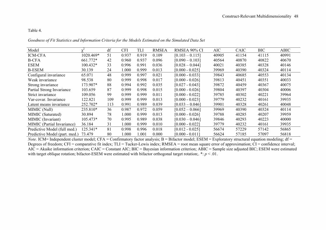
Construct-Relevant Multidimensionality 48
Table 4.
Goodness of Fit Statistics and Information Criteria for the Models Estimated on the Simulated Data Set
Model χ2 df CFI TLI RMSEA RMSEA 90% CI AIC CAIC BIC ABIC ICM-CFA 1020.469* 51 0.937 0.919 0.109 [0.103 – 0.115] 40905 41154 41115 40991 B-CFA 661.772* 42 0.960 0.937 0.096 [0.090 – 0.103] 40564 40870 40822 40670 ESEM 100.432* 33 0.996 0.991 0.036 [0.028 – 0.044] 40021 40385 40328 40146 B-ESEM 30.139 24 1.000 0.999 0.013 [0.000 - 0.025] 39969 40390 40324 40114 Configural invariance 65.071 48 0.999 0.997 0.021 [0.000 - 0.033] 39843 40685 40553 40134 Weak invariance 98.538 80 0.999 0.998 0.017 [0.000 - 0.026] 39813 40451 40351 40033 Strong invariance 173.907* 88 0.994 0.992 0.035 [0.027 - 0.043] 39872 40459 40367 40075 Partial Strong Invariance 103.659 87 0.999 0.998 0.015 [0.000 - 0.026] 39804 40397 40304 40006 Strict invariance 109.056 99 0.999 0.999 0.011 [0.000 - 0.022] 39785 40302 40221 39964 Var-covar. Invariance 122.821 109 0.999 0.999 0.013 [0.000 - 0.023] 39779 40232 40161 39935 Latent means invariance 252.702* 113 0.991 0.989 0.039 [0.033 – 0.046] 39901 40328 40261 40048 MIMIC (Null) 235.810* 36 0.987 0.972 0.059 [0.052 – 0.066] 39969 40390 40324 40114 MIMIC (Saturated) 30.894 78 1.000 0.999 0.013 [0.000 - 0.026] 39788 40285 40207 39959 MIMIC (Invariant) 105.473* 70 0.995 0.989 0.038 [0.030 – 0.046] 39846 40293 40223 40000 MIMIC (Partial Invariance) 36.184 31 1.000 0.999 0.010 [0.000 - 0.022] 39779 40232 40161 39935 Predictive Model (full med.) 125.341* 81 0.998 0.996 0.018 [0.012 - 0.025] 56674 57229 57142 56865 Predictive Model (part. med.) 73.479 80 1.000 1.001 0.000 [0.000 - 0.011] 56624 57185 57097 56818 Note. ICM= Independent cluster model; CFA = Confirmatory factor analysis; B = Bifactor model; ESEM = Exploratory structural equation modeling; df = Degrees of freedom; CFI = comparative fit index; TLI = Tucker-Lewis index; RMSEA = root mean square error of approximation; CI = confidence interval; AIC = Akaike information criterion; CAIC = Constant AIC; BIC = Bayesian information criterion; ABIC = Sample size adjusted BIC; ESEM were estimated with target oblique rotation; bifactor-ESEM were estimated with bifactor orthogonal target rotation;. *: p < .01.

Construct-Relevant Multidimensionality 49
Table 5.
Standardized Factor Correlations for the CFA (above the diagonal) and ESEM (below the diagonal) solutions for the Simulated Data Set
Factor 1 Factor 2 Factor 3 Factor 1 0.516** 0.613** Factor 2 0.475** 0.731** Factor 3 0.522** 0.629** Note. * p < .05. ** p < .01
Table 6.
Standardized Factor Loadings for Bifactor-ESEM Solution for the Simulated Data
Items G-Factor Loadings
S-Factor1 Loadings
S-Factor2 Loadings
S-Factor3 Loadings
Uniquenesses
X1 0.469** 0.602** -0.063* 0.100** 0.403**X2 0.466** 0.691** 0.176** 0.008 0.273**X3 0.663** 0.521** -0.176** -0.023 0.258**X4 0.639** 0.556** -0.050* -0.096** 0.271**Y1 0.661** -0.023 0.533** 0.134** 0.261**Y2 0.692** 0.130** 0.477** -0.015 0.276**Y3 0.747** -0.119** 0.546** 0.005 0.130**Y4 0.745** -0.042** 0.498** -0.075** 0.190**Z1 0.789** 0.128** -0.006 0.369** 0.225**Z2 0.791** -0.011 0.174** 0.353** 0.219**Z3 0.659** 0.005 -0.087** 0.552** 0.253**Z4 0.644** -0.079** 0.031* 0.583** 0.238*** p < .05. ** p < .01