Rule and Preference Learning -...
83
J. Fürnkranz Introduction to Machine Learning Rule and Preference Learning
Transcript of Rule and Preference Learning -...

J. Fürnkranz
Introduction to Machine Learning
Rule and Preference Learning
Johannes FürnkranzSummer School on Logic, AI and Verification | Machine Learning 2
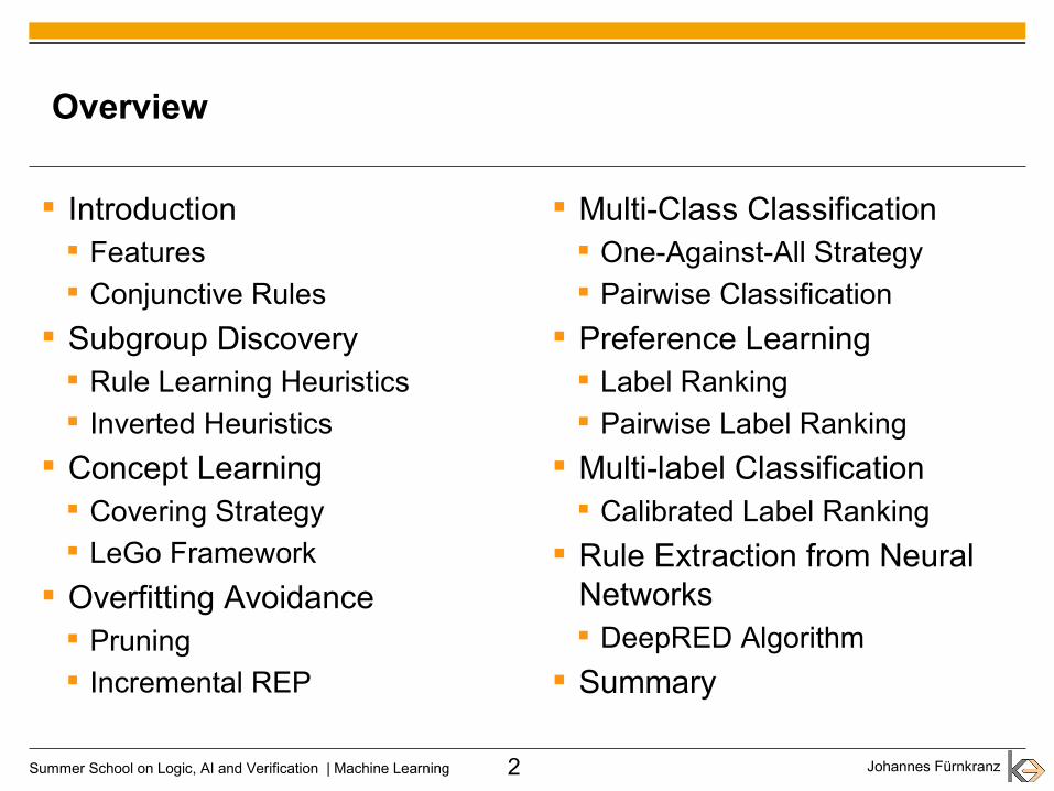
Overview
Introduction Features Conjunctive Rules
Subgroup Discovery Rule Learning Heuristics Inverted Heuristics
Concept Learning Covering Strategy LeGo Framework
Overfitting Avoidance Pruning Incremental REP
Multi-Class Classification One-Against-All Strategy Pairwise Classification
Preference Learning Label Ranking Pairwise Label Ranking
Multi-label Classification Calibrated Label Ranking
Rule Extraction from Neural Networks DeepRED Algorithm
Summary

Johannes FürnkranzSummer School on Logic, AI and Verification | Machine Learning 3
Supervised Learning - Induction of Classifiers
Training
ClassificationExample
Inductive Machine Learning algorithms
induce a classifier from labeled training examples. The classifier generalizes the training examples, i.e. it is able to assign labels
to new cases.
An inductive learning algorithm searches in a
given family of hypotheses (e.g., decision trees, neural networks) for a member that
optimizes given quality criteria (e.g., estimated predictive accuracy or
misclassification costs).
Classifier

Johannes FürnkranzSummer School on Logic, AI and Verification | Machine Learning 4
Why Rules?
Rules provide a good (the best?) trade-off between human understandability machine executability
Used in many applicationswhich will gain importance in the near future Security Spam Mail Filters Semantic Web
But they are not a universal tool e.g., learned rules sometimes lack in predictive accuracy
→ challenge to close or narrow this gap
Johannes FürnkranzSummer School on Logic, AI and Verification | Machine Learning 5
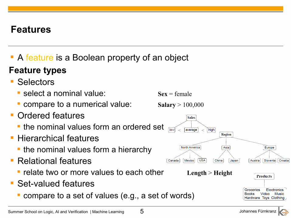
Features
A feature is a Boolean property of an object
Feature types Selectors select a nominal value: Sex = female
compare to a numerical value: Salary > 100,000
Ordered features the nominal values form an ordered set
Hierarchical features the nominal values form a hierarchy
Relational features relate two or more values to each other Length > Height
Set-valued features compare to a set of values (e.g., a set of words)

Johannes FürnkranzSummer School on Logic, AI and Verification | Machine Learning 6
Conjunctive Rule
Coverage A rule is said to cover an example if the example satisfies the
conditions of the rule.
Prediction If a rule covers an example, the rule's head is predicted for this example.
if (feature 1) and (feature 2) then +
Body of the rule (IF-part)● contains a conjunction of
conditions● a condition is a binary
feature
Head of the rule (THEN-part)● contains a prediction● typically + if object
belongs to concept,– otherwise

Johannes FürnkranzSummer School on Logic, AI and Verification | Machine Learning 7
A Sample Database
No. Education Marital S. Sex. Children? Approved?
1 Primary Single M N -
2 Primary Single M Y -
3 Primary Married M N +
4 University Divorced F N +
5 University Married F Y +
6 Secondary Single M N -
7 University Single F N +
8 Secondary Divorced F N +
9 Secondary Single F Y +
10 Secondary Married M Y +
11 Primary Married F N +
12 Secondary Divorced M Y -
13 University Divorced F Y -
14 Secondary Divorced M N +
Property of Interest(“class variable”)

Johannes FürnkranzSummer School on Logic, AI and Verification | Machine Learning 8
Subgroup Discovery
Definition
Examples
“Given a population of individuals and a property of those individuals that weare interested in, find population subgroups that are statistically 'most interesting', e.g., are as large as possible and have the most unusualdistributional characteristics with respect to the property of interest”
(Klösgen 1996; Wrobel 1997)

Johannes FürnkranzSummer School on Logic, AI and Verification | Machine Learning 9
Terminology
predicted + predicted -class + p (true positives) P-p (false negatives) P
class - n (false positives) N-n (true negatives) N
p + n P+N – (p+n) P+N
training examples P: total number of positive examples N: total number of negative examples
examples covered by the rule (predicted positive) true positives p: positive examples covered by the rule false positives n: negative examples covered by the rule
examples not covered the rule (predicted negative) false negatives P-p: positive examples not covered by the rule true negatives N-n: negative examples not covered by the rule

Johannes FürnkranzSummer School on Logic, AI and Verification | Machine Learning 10
Algorithms for Subgroup Discovery
Objective Find the best subgroups / rules according to some measure h
Algorithms Greedy search top-down hill-climbing or beam search successively add conditions that increase value of h most popular approach
Exhaustive search efficient variants avoid to search permutations of conditions more than once exploit monotonicity properties for pruning of parts of the search space
Randomized search genetic algorithms etc.

Johannes FürnkranzSummer School on Logic, AI and Verification | Machine Learning 11
Top-Down Hill-Climbing
Top-Down Strategy: A rule is successively specialized
1. Start with the universal rule R that covers all examples
2. Evaluate all possible ways to add a condition to R
3. Choose the best one (according to some heuristic)
4. If R is satisfactory, return it
5. Else goto 2.
Most greedy s&c rule learning systems use a top-down strategy
Beam Search: Always remember (and refine) the best b solutions in parallel
Johannes FürnkranzSummer School on Logic, AI and Verification | Machine Learning 12
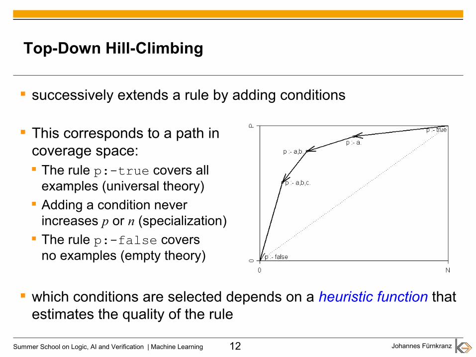
Top-Down Hill-Climbing
successively extends a rule by adding conditions
This corresponds to a path in coverage space: The rule p:-true covers all
examples (universal theory) Adding a condition never
increases p or n (specialization) The rule p:-false covers
no examples (empty theory)
which conditions are selected depends on a heuristic function that estimates the quality of the rule

Johannes FürnkranzSummer School on Logic, AI and Verification | Machine Learning 13
Rule Learning Heuristics
How can we measure the quality of a rule?
should cover as few negative examples as possible (consistency)
should cover as many positive examples as possible (completeness)
An evaluation heuristic should therefore trade off these two properties
Example: Laplace heuristic
grows with
grows with
Example: Precision
is not a good heuristic. Why?
hLap=p1
pn2
hPrec=p
pn
p∞
n0

Johannes FürnkranzSummer School on Logic, AI and Verification | Machine Learning 14
Example
2 2 0.5000 0.5000 03 1 0.7500 0.6667 24 2 0.6667 0.6250 22 3 0.4000 0.4286 -14 0 1.0000 0.8333 43 2 0.6000 0.5714 13 4 0.4286 0.4444 -16 1 0.8571 0.7778 53 3 0.5000 0.5000 06 2 0.7500 0.7000 4
Condition p n Precision Laplace p-nPrimary
Education = UniversitySecondarySingle
Marital Status = MarriedDivorced
Sex = MaleFemale
Children = YesNo
Heuristics Precision and Laplace add the condition Marital S. = Married to the (empty) rule stop and try to learn the next rule
Heuristic Accuracy / p − n adds Sex = Female continue to refine the rule (until no covered negative)

Johannes FürnkranzSummer School on Logic, AI and Verification | Machine Learning 15
3d-Visualization of Precision
2d Coverage Space

Johannes FürnkranzSummer School on Logic, AI and Verification | Machine Learning 16
Coverage Spaces
good tool for visualizing properties of rule evaluation heuristics each point is a rule covering p positive and n negative examples
universal rule:all examples are covered
(most general)
empty rule:no examples are covered
(most specific)
perfect rule:all positive and
no negativeexamples
are covered
random rules:predict with
coin tosses withfixed probability
opposite rule:all negative and
no positive examples
are covered
iso-accuracy:cover sameamount ofpositive
and negativeexamples

Johannes FürnkranzSummer School on Logic, AI and Verification | Machine Learning 17
Isometrics in Coverage Space
Isometrics are lines that connect points for which a function in p and n has equal values
Examples: Isometrics for heuristics h
p = p and h
n = -n

Johannes FürnkranzSummer School on Logic, AI and Verification | Machine Learning 18
Precision
basic idea: percentage of
positive examples among covered examples
effects: rotation around
origin (0,0) all rules with same
angle equivalent in particular, all
rules on P/N axes are equivalent
typically overfits
hPrec=p
pn
Johannes FürnkranzSummer School on Logic, AI and Verification | Machine Learning 19
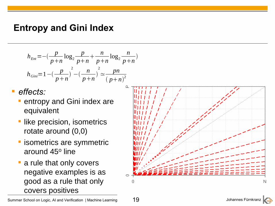
Entropy and Gini Index
effects: entropy and Gini index are
equivalent
like precision, isometrics rotate around (0,0)
isometrics are symmetric around 45o line
a rule that only covers negative examples is as good as a rule that only covers positives
hEnt=−p
pnlog2
ppn
n
pnlog2
npn
hGini=1−p
pn
2
−n
pn
2
≃pn
pn2

Johannes FürnkranzSummer School on Logic, AI and Verification | Machine Learning 20
Accuracy
basic idea:percentage of correct classifications (covered positives plus uncovered negatives)
effects: isometrics are parallel
to 45o line covering one positive
example is as good as not covering one negative example
hAcc=pN−n
PN≃ p−n Why are they
equivalent?
hAcc=P
PN
hAcc=N
PN
hAcc=12

Johannes FürnkranzSummer School on Logic, AI and Verification | Machine Learning 21
Weighted Relative Accuracy
Two Basic ideas: Precision Gain: compare precision to precision of a rule that classifies
all examples as positive
Coverage: Multiply with the percentage of covered examples
Resulting formula:
one can show that sorts rules in exactly the same way as
ppn
−P
PN
pnPN
hWRA=pn
PN⋅ p
pn−
PPN
hWRA '=pP−
nN

Johannes FürnkranzSummer School on Logic, AI and Verification | Machine Learning 22
Weighted relative accuracy
basic idea:compte the distance fromthe diagonal (i.e., from random rules)
effects: isometrics are parallel
to diagonal covering x% of the
positive examples isconsidered to be as good as not covering x% of the negative examples
typically over-generalizes
hWRA=p+ n
P+ N (p
p+ n−
PP+ N )≃
pP−
nN
hWRA=0

Johannes FürnkranzSummer School on Logic, AI and Verification | Machine Learning 25
Laplace-Estimate
basic idea:precision, but count coverage for positive and negative examples starting with 1 instead of 0
effects: origin at (-1,-1) different values on
p=0 or n=0 axes not equivalent to
precision
hLap=p1
p1n1=
p1pn2

Johannes FürnkranzSummer School on Logic, AI and Verification | Machine Learning 26
m-estimate
basic idea:initialize the counts with m examples in total, distributed according to the prior distribution P/(P+N) of p and n.
effects: origin shifts to
(-mP/(P+N),-mN/(P+N)) with increasing m, the
lines become more and more parallel
can be re-interpreted as a trade-off between WRA and precision/confidence
hm=
p+ mP
P+ N
( p+ mP
P+ N )+ (n+ mN
P+ N )=
p+ mP
P+ Np+ n+ m

Johannes FürnkranzSummer School on Logic, AI and Verification | Machine Learning 31
Non-Linear Isometrics – Correlation
basic idea:measure correlation coefficient of predictions with target
effects: non-linear isometrics in comparison to WRA prefers rules near the
edges steepness of connection of
intersections with edges increases
equivalent to χ2
hCorr=p N−n−P− pn
PN pnP− pN−n

Johannes FürnkranzSummer School on Logic, AI and Verification | Machine Learning 33
Application Study: Life Course Analysis
Data: Fertility and Family Survey 1995/96 for Italians and Austrians Features based on general descriptors and variables that describes
whether (quantum), at which age (timing) and in what order (sequencing) typical life course events have occurred.
Objective: Find subgroups that capture typical life courses for either country
Examples:

Johannes FürnkranzSummer School on Logic, AI and Verification | Machine Learning 34
Inverted Heuristics – Motivation
While the search proceeds top-down the evaluation of refinements happens from the point of view of
the origin (bottom-up)
Instead, we want to evaluate the refinement from the point of view of the predecessor
Johannes FürnkranzSummer School on Logic, AI and Verification | Machine Learning 35
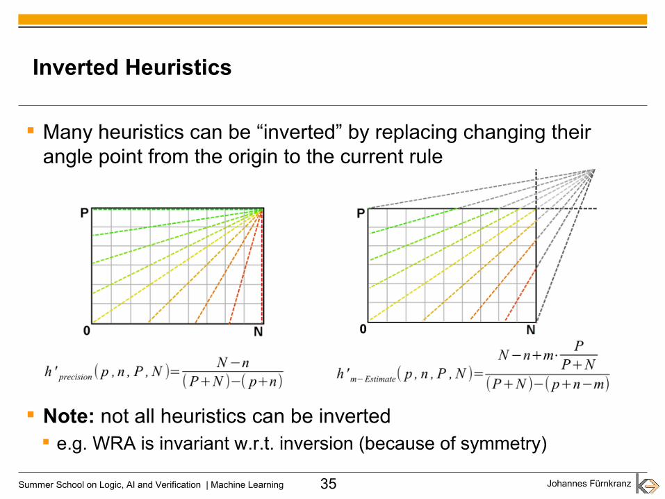
Inverted Heuristics
Many heuristics can be “inverted” by replacing changing their angle point from the origin to the current rule
Note: not all heuristics can be inverted e.g. WRA is invariant w.r.t. inversion (because of symmetry)

Johannes FürnkranzSummer School on Logic, AI and Verification | Machine Learning 36
Inverted Heuristics – Example

Johannes FürnkranzSummer School on Logic, AI and Verification | Machine Learning 37
Example: Mushroom dataset
The best three rules learned with conventional heuristics
The best three rules learned with inverted heuristics
IF veil-color = w, gill-spacing = c, bruises? = f, ring-number = o, stalk-surface-above-ring = kTHEN poisonous (2192,0)IF veil-color = w, gill-spacing = c, gill-size = n, population = v, stalk-shape = tTHEN poisonous (864,0)IF stalk-color-below-ring = w, ring-type = p, stalk-color-above-ring = w, ring-number = o, cap-surface = s, stalk-root = b, gill-spacing = cTHEN poisonous (336)
IF odor = f THEN poisonous (2160,0) IF gill-color = b THEN poisonous (1152,0) IF odor = p THEN poisonous (256,0)

Johannes FürnkranzSummer School on Logic, AI and Verification | Machine Learning 38
Inverted Heuristics – Rule Length
Inverted Heuristics tend to learn longer rules If there are conditions that can be added without decreasing coverage,
inverted heuristics will add them first (before adding discriminative conditions)
Typical intuition: long rules are less understandable, therefore short rules are preferable short rules are more general, therefore (statistically) more reliable
Should shorter rules be preferred? Claim: Not necessarily, because longer rules may capture more
information about the object Related to discriminative rules vs. characteristic rules Open question...

Johannes FürnkranzSummer School on Logic, AI and Verification | Machine Learning 39
Discriminative Rules
Allow to quickly discriminate an object of one category from objects of other categories
Typically a few properties suffice
Example:

Johannes FürnkranzSummer School on Logic, AI and Verification | Machine Learning 40
Characteristic Rules
Allow to characterize an object of a category Focus is on all properties that are representative for objects of
that category
Example:
Johannes FürnkranzSummer School on Logic, AI and Verification | Machine Learning 41
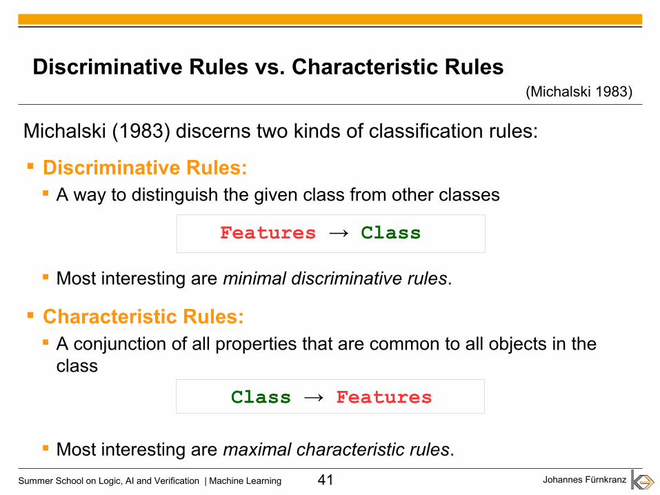
Discriminative Rules vs. Characteristic Rules
Michalski (1983) discerns two kinds of classification rules:
Discriminative Rules: A way to distinguish the given class from other classes
Most interesting are minimal discriminative rules.
Characteristic Rules: A conjunction of all properties that are common to all objects in the
class
Most interesting are maximal characteristic rules.
(Michalski 1983)
Features → Class
Class → Features

Johannes FürnkranzSummer School on Logic, AI and Verification | Machine Learning 42
Characteristic Rules
An alternative view of characteristic rules is to invert the implication sign
All properties that are implied by the category
Example:

Johannes FürnkranzSummer School on Logic, AI and Verification | Machine Learning 43
From Descriptive Rules to Predictive Theories
Descriptive Learning Focus on discovering patterns that describe (parts of) the data
Predictive Learning Focus on finding patterns that allow to make predictions about the data
From Descriptive Rules to Predictive Rule Sets Rule Diversity and Completeness: We need to be able to make a prediction for every possible instance
Predictive Evaluation: It is important how well rules are able to predict the dependent variable
on new data

Johannes FürnkranzSummer School on Logic, AI and Verification | Machine Learning 44
Concept Learning
Given: Positive Examples E+
examples for the concept to learn (e.g., days with golf)
Negative Examples E
counter-examples for the concept (e.g., days without golf)
Hypothesis Space H a (possibly infinite) set of candidate hypotheses e.g., rules, rule sets, decision trees, linear functions, neural networks, ...
Find: Find the target hypothesis h ∈ H the target hypothesis is the concept that was used (or could have been
used) to generate the training examples

Johannes FürnkranzSummer School on Logic, AI and Verification | Machine Learning 45
A Learned Rule Set
IF E=primary AND S=male AND M=married AND C=no THEN yes IF E=university AND S=female AND M=divorced AND C=no THEN yes IF E=university AND S=female AND M=married AND C=yes THEN yes IF E=university AND S=female AND M=single AND C=no THEN yes IF E=secondary AND S=female AND M=divorced AND C=no THEN yes IF E=secondary AND S=female AND M=single AND C=yes THEN yes IF E=secondary AND S=male AND M=married AND C=yes THEN yes IF E=primary AND S=female AND M=married AND C=no THEN yes IF E=secondary AND S=male AND M=divorced AND C=no THEN yesELSE no
IF E=primary AND S=male AND M=married AND C=no THEN yes IF E=university AND S=female AND M=divorced AND C=no THEN yes IF E=university AND S=female AND M=married AND C=yes THEN yes IF E=university AND S=female AND M=single AND C=no THEN yes IF E=secondary AND S=female AND M=divorced AND C=no THEN yes IF E=secondary AND S=female AND M=single AND C=yes THEN yes IF E=secondary AND S=male AND M=married AND C=yes THEN yes IF E=primary AND S=female AND M=married AND C=no THEN yes IF E=secondary AND S=male AND M=divorced AND C=no THEN yesELSE no
The solution is a set of rules that is complete and consistent on the training examples
→ it must be part of the version space but it does not generalize to new examples!

Johannes FürnkranzSummer School on Logic, AI and Verification | Machine Learning 46
A Better Solution
IF Marital = married THEN yes
IF Marital = single AND Sex = female THEN yes
IF Marital = divorced AND Children = no THEN yes
ELSE no
IF Marital = married THEN yes
IF Marital = single AND Sex = female THEN yes
IF Marital = divorced AND Children = no THEN yes
ELSE no

Johannes FürnkranzSummer School on Logic, AI and Verification | Machine Learning 47
Separate-and-Conquer Rule Learning
Learn a set of rules, one rule after the other using greedy covering
1. Start with an empty theory T and training set E2. Learn a single (consistent) rule R from E and add it to T 3. If T is satisfactory (complete), return T4. Else:
Separate: Remove examples explained by R from EConquer: goto 2.
One of the oldest family of learning algorithms Different learners differ in how they find a single rule Completeness and consistency requirements are typically
loosened

Johannes FürnkranzSummer School on Logic, AI and Verification | Machine Learning 49
Covering Strategy
Covering or Separate-and-Conquer rule learning learning algorithms learn one rule at a time and then removes the examples covered by this rule
This corresponds to a pathin coverage space: The empty theory R0 (no rules)
corresponds to (0,0) Adding one rule never
decreases p or n because adding a rule covers more examples (generalization)
The universal theory R+ (all examples are positive) corresponds to (N,P)
+

Johannes FürnkranzSummer School on Logic, AI and Verification | Machine Learning 51
Which Heuristic is Best?
There have been many proposals for different heuristics and many different justifications for these proposals some measures perform better on some datasets, others on other
datasets
Large-Scale Empirical Comparison: 27 training datasets on which parameters of the heuristics were tuned)
30 independent datasets which were not seen during optimization
Goals: see which heuristics perform best determine good parameter values for parametrized functions

Johannes FürnkranzSummer School on Logic, AI and Verification | Machine Learning 52
Empirical Comparison of Different Heuristics
Training
84,96 16,93 78,97 12,2085,63 26,11 78,87 25,3085,87 48,26 78,67 46,3383,68 37,48 77,54 47,33
Laplace 82,28 91,81 76,87 117,0082,36 101,63 76,22 128,3782,68 106,30 76,07 122,87
WRA 82,87 14,22 75,82 12,0082,24 85,93 75,65 99,13
Datasets Independent DatasetsHeuristic Accuracy # Conditions Accuracy #ConditionsRipper (JRip)Relative Cost Metric (c =0.342)m-Estimate (m = 22.466)Correlation
PrecisionLinear Cost Metric (c = 0.437)
Accuracy
Ripper is best, but uses pruning (the others don't) the optimized parameters for the m-estimate and the relative cost
metric perform better than all other heuristics also on the 30 datasets on which they were not optimized
some heuristics clearly overfit (bad performance with large rules) WRA over-generalizes (bad performance with small rules)

Johannes FürnkranzSummer School on Logic, AI and Verification | Machine Learning 53
Best Parameter Settings
for m-estimate: m = 22.5
meta-learned with a NN
Johannes FürnkranzSummer School on Logic, AI and Verification | Machine Learning 60
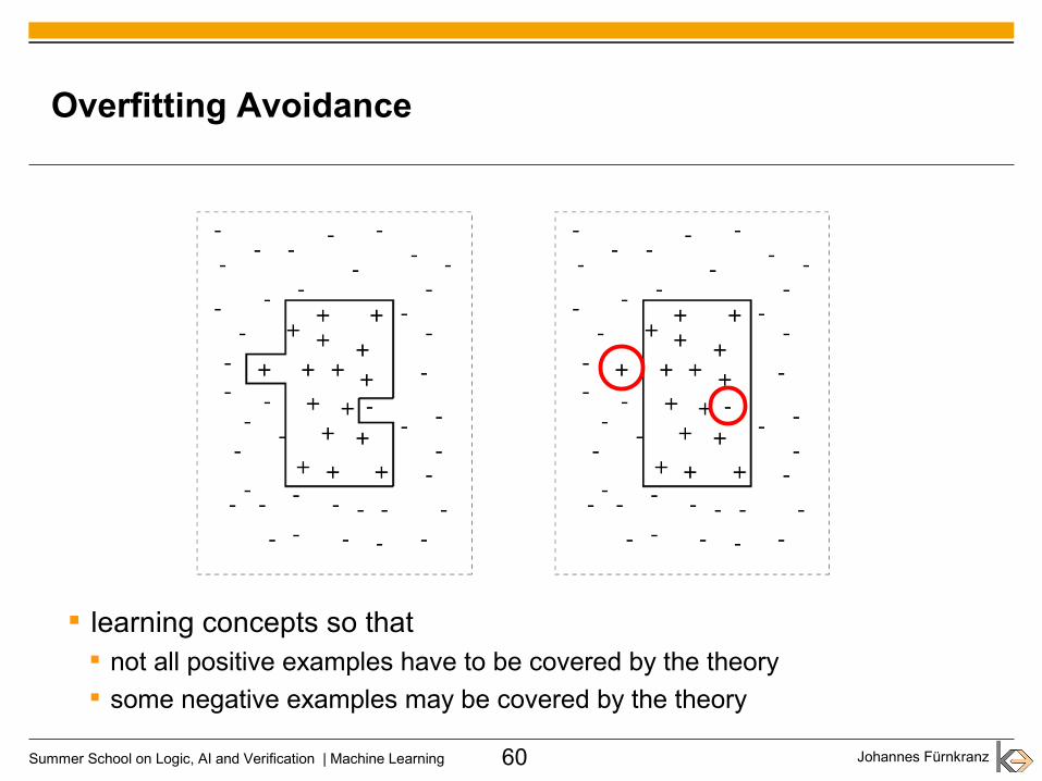
Overfitting Avoidance
learning concepts so that not all positive examples have to be covered by the theory some negative examples may be covered by the theory

Johannes FürnkranzSummer School on Logic, AI and Verification | Machine Learning 61
Complexity of Concepts
For simpler concepts there is less danger that they are able to overfit the data for a polynomial of degree n one can choose n+1 parameters in order
to fit the data points
→ many learning algorithms focus on learning simple concepts a short rule that covers many positive examples (but possibly also a
few negatives) is often better than a long rule that covers only a few positive examples
Pruning: Complex rules will be simplified Pre-Pruning: during learning
Post-Pruning: after learning

Johannes FürnkranzSummer School on Logic, AI and Verification | Machine Learning 74
Post-Pruning: Example
IF E=primary AND S=male AND M=single AND C=no THEN noIF E=primary AND S=male AND M=single AND C=yes THEN no IF E=primary AND S=male AND M=married AND C=no THEN yes IF E=university AND S=female AND M=divorced AND C=no THEN yes IF E=university AND S=female AND M=married AND C=yes THEN yes IF E=secondary AND S=male AND M=single AND C=no THEN no IF E=university AND S=female AND M=single AND C=no THEN yes IF E=secondary AND S=female AND M=divorced AND C=no THEN yes IF E=secondary AND S=female AND M=single AND C=yes THEN yes IF E=secondary AND S=male AND M=married AND C=yes THEN yes IF E=primary AND S=female AND M=married AND C=no THEN yes IF E=secondary AND S=male AND M=divorced AND C=yes THEN no IF E=university AND S=female AND M=divorced AND C=yes THEN no IF E=secondary AND S=male AND M=divorced AND C=no THEN yes
IF E=primary AND S=male AND M=single AND C=no THEN noIF E=primary AND S=male AND M=single AND C=yes THEN no IF E=primary AND S=male AND M=married AND C=no THEN yes IF E=university AND S=female AND M=divorced AND C=no THEN yes IF E=university AND S=female AND M=married AND C=yes THEN yes IF E=secondary AND S=male AND M=single AND C=no THEN no IF E=university AND S=female AND M=single AND C=no THEN yes IF E=secondary AND S=female AND M=divorced AND C=no THEN yes IF E=secondary AND S=female AND M=single AND C=yes THEN yes IF E=secondary AND S=male AND M=married AND C=yes THEN yes IF E=primary AND S=female AND M=married AND C=no THEN yes IF E=secondary AND S=male AND M=divorced AND C=yes THEN no IF E=university AND S=female AND M=divorced AND C=yes THEN no IF E=secondary AND S=male AND M=divorced AND C=no THEN yes

Johannes FürnkranzSummer School on Logic, AI and Verification | Machine Learning 75
IF S=male AND M=single THEN no
IF M=divorced AND C=yes THEN no
ELSE yes
IF S=male AND M=single THEN no
IF M=divorced AND C=yes THEN no
ELSE yes
Post-Pruning: Example

Johannes FürnkranzSummer School on Logic, AI and Verification | Machine Learning 76
Reduced Error Pruning
basic idea optimize the accuracy of a rule set on a separate pruning set
1. split training data into a growing and a pruning set
2. learn a complete and consistent rule set covering all positive examples and no negative examples
3. as long as the error on the pruning set does not increase delete condition or rule that results in the largest reduction of error on the
pruning set
4. return the remaining rules
REP is accurate but not efficient O(n4)

Johannes FürnkranzSummer School on Logic, AI and Verification | Machine Learning 80
Multi-Class Classification
No. Education Marital S. Sex. Children? Car
1 Primary Single M N Sports
2 Primary Single M Y Family
3 Primary Married M N Sports
4 University Divorced F N Mini
5 University Married F Y Mini
6 Secondary Single M N Sports
7 University Single F N Mini
8 Secondary Divorced F N Mini
9 Secondary Single F Y Mini
10 Secondary Married M Y Family
11 Primary Married F N Mini
12 Secondary Divorced M Y Family
13 University Divorced F Y Sports
14 Secondary Divorced M N Sports
Property of Interest(“class variable”)

Johannes FürnkranzSummer School on Logic, AI and Verification | Machine Learning 81
Learning Multiclass Classifiers
A1 A2 A3 Label
1 1 1 a
1 1 0 c
1 0 1 c
1 0 0 b
0 0 0 c
0 1 0 c
0 1 1 a
example withunknown class label
Classifier
dataset with class label for each example
A1 A2 A3 Label
0 0 1 b
A1 A2 A3 Label
0 0 1 ?

Johannes FürnkranzSummer School on Logic, AI and Verification | Machine Learning 82
Multi-Class Classification
Can we solve multi-classproblems with what wealready know (by reducingthem to binary problems)?

Johannes FürnkranzSummer School on Logic, AI and Verification | Machine Learning 83
One-against-all Reduction
c binary problems, one for each class label examples of class positive, all others negative

Johannes FürnkranzSummer School on Logic, AI and Verification | Machine Learning 84
Pairwise Reduction
c(c-1)/2 problems each class against each
other class
smaller training sets simpler decision boundaries larger margins

Johannes FürnkranzSummer School on Logic, AI and Verification | Machine Learning 85
Aggregating Pairwise Predictions
Aggregate the predictions of the binary classifiers into a final ranking by computing a score si for each class i
Voting: count the number of predictions for each class (number of points in a tournament)
Weighted Voting: weight the predictions by their probability
General Pairwise Coupling problem: Given for all i, j Find for all i Can be turned into an (underconstrained) system of linear equations
si=∑j≠i
δ {P (i> j)>0.5} {x }={1 if x= true 0 if x= false
P (i> j)
si=∑j=1
c
P (i> j)
P (i> j)=P (i ∣ i , j )P i

Johannes FürnkranzSummer School on Logic, AI and Verification | Machine Learning 86
Pairwise Classification & Ranking Loss
➔Weighted Voting optimizes Spearman Rank Correlation assuming that pairwise probabilities are estimated correctly
➔Kendall's Tau can in principle be optimized problem is NP-complete, but can be approximated
Different ways of combining the predictions of the binary classifiers optimize different loss functions without the need for re-training of the binary classifiers!
However, not all loss functions can be optimized e.g., 0/1 loss for rankings cannot be optimized or in general the probability distribution over the rankings cannot be
recovered from pairwise information

Johannes FürnkranzSummer School on Logic, AI and Verification | Machine Learning 87
Performance of Pairwise Classification
error rates on 20 benchmark data sets with 4 or more classes 10 significantly better
(p > 0.99, McNemar) 2 significantly better
(p > 0.95) 8 equal never (significantly)
worse
one-vs-all pairwise
Johannes FürnkranzSummer School on Logic, AI and Verification | Machine Learning 88
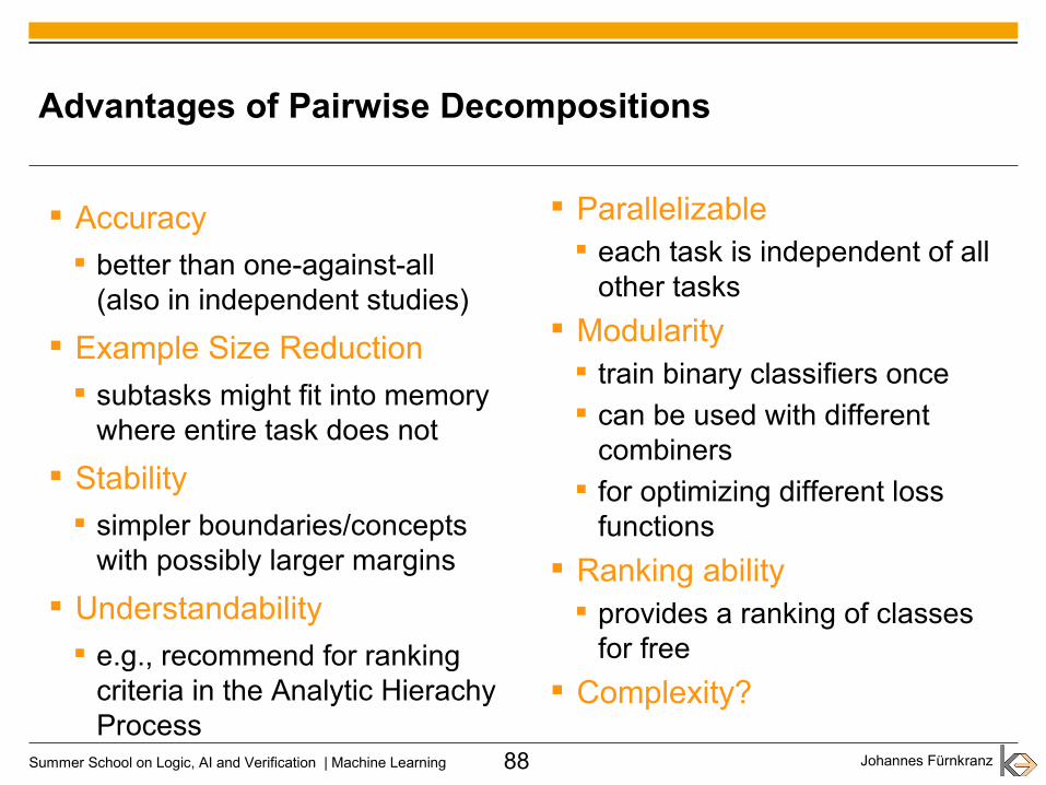
Accuracy better than one-against-all
(also in independent studies)
Example Size Reduction subtasks might fit into memory
where entire task does not
Stability simpler boundaries/concepts
with possibly larger margins
Understandability e.g., recommend for ranking
criteria in the Analytic Hierachy Process
Parallelizable each task is independent of all
other tasks
Modularity train binary classifiers once can be used with different
combiners for optimizing different loss
functions
Ranking ability provides a ranking of classes
for free
Complexity?
Advantages of Pairwise Decompositions

Johannes FürnkranzSummer School on Logic, AI and Verification | Machine Learning 89
Proof: ● each of the n training examples occurs in all binary tasks where its class is
paired with one of the other c−1 classes
Training Complexity of Pairwise Classification
Lemma: The total number of training examples for all binary classifiers in a pairwise classification ensemble is (c–1)∙n
Lemma: The total number of training examples for all binary classifiers in a pairwise classification ensemble is (c–1)∙n
Proof Sketch: ● one-against-all binarization needs a total of c∙n examples● fewer training examples are distributed over more classifiers● more small training sets are faster to train than few large training sets● for complexity f(n) = no (o > 1): o1∑ ni
o∑ ni
o
Theorem: For learning algorithms with at least linear complexity, pairwise classification is more efficient than one-against-all.
Theorem: For learning algorithms with at least linear complexity, pairwise classification is more efficient than one-against-all.

Johannes FürnkranzSummer School on Logic, AI and Verification | Machine Learning 90
Preference Data
No. Education Marital S. Sex. Children? Car Preferences
1 Primary Single M N Sports > Family
2 Primary Single M Y Family > Sports, Family > Mini
3 Primary Married M N Sports > Family > Mini
4 University Divorced F N Mini > Family
5 University Married F Y Mini > Sports
6 Secondary Single M N Sports > Mini > Family
7 University Single F N Mini > Family, Mini > Sports
8 Secondary Divorced F N Mini > Sports
9 Secondary Single F Y Mini > Sports, Family > Sports
10 Secondary Married M Y Family > Mini
11 Primary Married F N Mini > Family
12 Secondary Divorced M Y Family > Sports > Mini
13 University Divorced F Y Sports > Mini, Family > Mini
14 Secondary Divorced M N Sports > Mini

Johannes FürnkranzSummer School on Logic, AI and Verification | Machine Learning 91
Class Information encodes Preferences
A1 A2 A3 Label Pref.
1 1 1 a a > b | a > c
1 1 0 c c > b | c > a
1 0 1 c c > b | c > a
1 0 0 b b > a | b > c
0 0 0 c c > b | c > a
0 1 0 c c > b | c > a
0 1 1 a a > b | a > c
example withunknown class label
A1 A2 A3 Label
0 0 1 b
A1 A2 A3 Label
0 0 1 ?
dataset with class label for each example
LabelPreference
Learner
a > b means: for this example label a is preferred over label b

Johannes FürnkranzSummer School on Logic, AI and Verification | Machine Learning 92
General Label Preference Learning Problem
A1 A2 A3 Pref.
1 1 1 a > b | b > c
1 1 0 a > b | c > b
1 0 1 b > a
1 0 0 b > a | a > c | c > b
0 0 0 c > a
0 1 0 c > b | c > a
0 1 1 a > c
example withunknown preferences Label
Preference Learner
dataset with preferences for each example
A1 A2 A3 Pref.
0 0 1 b > a > c
A1 A2 A3 Pref.
0 0 1 ?
Each examplemay have an arbitrary number of preferences
We typically predict a complete ranking
(a total order)

Johannes FürnkranzSummer School on Logic, AI and Verification | Machine Learning 93
Label Ranking
GIVEN: a set of labels: a set of contexts: for each training context ek: a set of preferences
FIND: a label ranking function that orders the labels for any given
context
GIVEN: a set of labels: a set of contexts: for each training context ek: a set of preferences
FIND: a label ranking function that orders the labels for any given
context
Pk={λi≻k λ j}⊆L x L
E={ek∣k=1n }
L={i∣i=1c }
Preference learning scenario in which contexts are characterized by features no information about the items is given except a unique name (a label)

Johannes FürnkranzSummer School on Logic, AI and Verification | Machine Learning 94
Pairwise Preference Learning

Johannes FürnkranzSummer School on Logic, AI and Verification | Machine Learning 95
A Multilabel Database
No. Education Marital S. Sex. Children? Quality Tabloid Fashion Sports
1 Primary Single M N 0 0 0 0
2 Primary Single M Y 0 0 0 1
3 Primary Married M N 0 0 0 0
4 University Divorced F N 1 1 1 0
5 University Married F Y 1 0 1 0
6 Secondary Single M N 0 1 0 0
7 University Single F N 1 1 0 0
8 Secondary Divorced F N 1 0 0 1
9 Secondary Single F Y 0 1 1 0
10 Secondary Married M Y 1 1 0 1
11 Primary Married F N 1 0 0 0
12 Secondary Divorced M Y 0 1 0 0
13 University Divorced F Y 0 1 1 0
14 Secondary Divorced M N 1 0 0 1

Johannes FürnkranzSummer School on Logic, AI and Verification | Machine Learning 96
Multi-Label Classification
Multilabel Classification: each context is associated with multiple labels e.g., keyword assignments to texts
Relevant labels R for an example those that should be assigned to the example
Irrelevant labels I = L \ R for an example those that should not be assigned to the examples
Simple solution: Predict each label independently (Binary Relevance / one-vs-all)
Key Challenge: The prediction tasks are not independent!

Johannes FürnkranzSummer School on Logic, AI and Verification | Machine Learning 97
Pairwise Multi-Label Ranking
Tranformation of Multi-Label Classification problems into preference learning problems is straight-forward
at prediction time, the pairwise ensemble predicts a label ranking
Problem:
Where to draw boundary between relevant and irrelevant labels?
relevant labels
irrelevant labels
|R|∙|I| preferences
λ7
λ4
λ6
λ2
λ5
λ1
λ3
R
I

Johannes FürnkranzSummer School on Logic, AI and Verification | Machine Learning 98
Calibrated Multi-Label PC
Key idea: introduce a neutral label into the preference scheme the neutral label is less relevant than all relevant classes more relevant than all irrelevant classes
at prediction time, all labels that are ranked abovethe neutral label are predicted to be relevant
λ7
λ4
λ6
λ2
λ5
λ1
λ3
λ0
neutral label c = |R| + |I| new preferences
R
I

Johannes FürnkranzSummer School on Logic, AI and Verification | Machine Learning 99
EuroVOC Classification of EC Legal Texts
Eur-Lex database ≈ 20,000 documents ≈ 4,000 labels ≈ 5 labels per document
Pairwise modeling approachlearns ≈8,000,000 perceptrons memory-efficient dual
representation necessary
Results: average precision of pairwise method is almost 50%
→ on average, the 5 relevant labels can be found within the first 10 labels of the ranking of all 4000 labels
one-against-all methods (BR and MMP) had an avg. precision < 30%

Johannes FürnkranzSummer School on Logic, AI and Verification | Machine Learning 101
Open Problems
Multilabel Rule Learning
The key challenge in multi-label classification is to model the dependencies between the labels
much of current research in this area is devoted to this topic
Rules can make these dependencies explicit and exploit them in the learning phase
regular rule: university, female → quality, fashion
label dependency: fashion ≠ sports
mixed rule: university, tabloid → quality

Johannes FürnkranzSummer School on Logic, AI and Verification | Machine Learning 106
Structured Concepts
Most rule learning algorithms learn flat theories e.g., n-bit parity needs 2n flat
rules
But structured concepts are often more interpretable e.g. only O(n) rules with
intermediate concepts
+ :- x1, x2, x3, x4.+ :- x1, x2, not x3, not x4.+ :- x1, not x2, x3, not x4.+ :- x1, not x2, not x3, x4.+ :- not x1, x2, not x3, x4.+ :- not x1, x2, x3, not x4.+ :- not x1, not x2, x3, x4.+ :- not x1, not x2, not x2, not x4.
Previous work in the 90s in inductive logic programming (ILP) and restructuring knowledge bases was not successful
new approaches could borrow ideas from Deep Learning
+ :- x1, not parity234.+ :- not x1, parity234.
parity234 :- x2, not parity34.parity234 :- not x2, parity34.
parity34 :- x3, x4.parity34 :- not x3, not x4.

Johannes FürnkranzSummer School on Logic, AI and Verification | Machine Learning 107
Rule Extraction from Neural Networks
Pedagogical Strategy: Train a (deep) network

Johannes FürnkranzSummer School on Logic, AI and Verification | Machine Learning 109
DeepRED: Rule Extraction from Deep Networks
(Zilke, Loza, Janssen 2016)
Step 1: Propagate activation through network

Johannes FürnkranzSummer School on Logic, AI and Verification | Machine Learning 110
DeepRED: Rule Extraction from Deep Networks
(Zilke, Loza, Janssen 2016)
Step 2: Find a decision tree that describes an output node using activation values of the previous hidden layer hi

Johannes FürnkranzSummer School on Logic, AI and Verification | Machine Learning 111
DeepRED: Rule Extraction from Deep Networks
(Zilke, Loza, Janssen 2016)
Step 3: Replace target activations hi
by split points on hi using in prediction model hi → hi+1

Johannes FürnkranzSummer School on Logic, AI and Verification | Machine Learning 112
DeepRED: Rule Extraction from Deep Networks
(Zilke, Loza, Janssen 2016)
Step 4: induce model hi-1 → hi
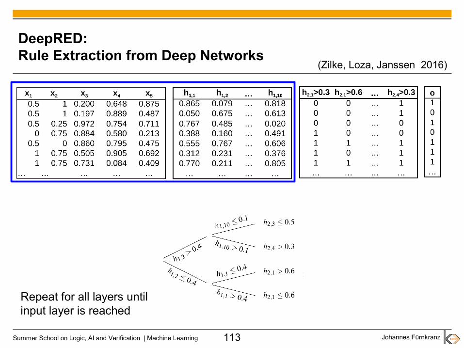
Johannes FürnkranzSummer School on Logic, AI and Verification | Machine Learning 113
DeepRED: Rule Extraction from Deep Networks
(Zilke, Loza, Janssen 2016)
Repeat for all layers until input layer is reached

Johannes FürnkranzSummer School on Logic, AI and Verification | Machine Learning 114
DeepRED: Rule Extraction from Deep Networks
(Zilke, Loza, Janssen 2016)

Johannes FürnkranzSummer School on Logic, AI and Verification | Machine Learning 115
DeepRED: Rule Extraction from Deep Networks
Represent output as a function of inputs
Extract rule sets R(hi-1 → hi) from decision trees
Optional: Combine rules into a single rule set Advance layerwise
put R(hi-1 → hi) into R(hi → ho) to get R(hi-1 → ho)
delete unsatisfiable and redundant terms
(Zilke, Loza, Janssen 2016)
IF x1>0.5 AND x2>0.6 THEN h11<=0.4IF x1>0.5 AND x2<=0.6 THEN h11>0.4IF x1<=0.5 …...
IF h12>0.4 AND h110<=0.1 THEN h23<=0.5IF h12>0.4 AND h110>0.1 THEN h24>0.3IF h12<=0.4 AND h11<=0.4 THEN h21>0.6IF h12<=0.4 AND h11 >0.1 THEN h21<=0.6
IF h21>0.6 AND h24>0.3 THEN o=0IF h21>0.6 AND h24<=0.3 THEN o=1IF h21<=0.6 THEN o=1

Johannes FürnkranzSummer School on Logic, AI and Verification | Machine Learning 116
Can DeepRED make use of complex concepts hidden in NNs?
XOR parity function: x ∈ {0,1}8 → XOR(x1,x2,x3,x4,x5,x6,x7,x8}
28 examples split into 150 training and 106 test examples top-down approaches (e.g. C4.5) usually need all examples to learn
consistent model
Results as expected, baseline fails DeepRED is able to extract
rules that classify all or almost all test examples correctly
Open Question Understandability of intermediate
concepts?
(Zilke, Loza, Janssen 2016)

Johannes FürnkranzSummer School on Logic, AI and Verification | Machine Learning 117
Summary (1)
Rules can be learned via top-down hill-climbing add one condition at a time until the rule covers no more negative exs.
Heuristics are needed for guiding the search can be visualize through isometrics in coverage space
Rule Sets can be learned one rule at a time using the covering or separate-and conquer strategy
Overfitting is a serious problem for all machine learning algorithms too close a fit to the training data may result in bad generalizations
Pruning can be used to fight overfitting Pre-pruning and post-pruning can be efficiently integrated
Multi-class problems can be addressed by multiple rule sets one-against-all classification or pairwise classification

Johannes FürnkranzSummer School on Logic, AI and Verification | Machine Learning 118
Summary (2)
Problem decomposition as a powerful tool Try to understand simple problems first Build solutions for complex problems on
well-understood solutions for simpler problems
motivated by research in rule learning but applied to other fields e.g., work on preference learning has (so far) used little rule learning
Preference Learning is a general framework for decomposing complex machine learning problems into simpler problems multi-label classification, graded ML classification,
ordered classification, hierarchical classification, ranking...
subgroup discovery → concept learning → multi-class classification → → preference learning → multi-label classification
subgroup discovery → concept learning → multi-class classification → → preference learning → multi-label classification

Johannes FürnkranzSummer School on Logic, AI and Verification | Machine Learning 119
Literatur
J. Fürnkranz, D. Gamberger, N. Lavrac, Foundations of Rule LearningSpringer-Verlag, 2012.
J. Fürnkranz, E. Hüllermeier (eds.) Preference Learning
Springer-Verlag, 2011.