RT SSV&A
290
Real-time Systems Specification, Verification and Analysis Edited by Mathai Joseph Tata Research Development & Design Centre Revised version with corrections June 2001
-
Upload
cara-sucia -
Category
Science
-
view
65 -
download
1
Transcript of RT SSV&A
Real-time SystemsSpecification, Verification and
Analysis
Edited by Mathai JosephTata Research Development & Design Centre
Revised version with correctionsJune 2001

Original edition published in 1996 by Prentice Hall International, London,underISBN 0-13-455297-0
This version incorporates corrections to and changes from the originaledition.
This version is madeavailable for research,teaching and personal useonly.
Copies may be made for non-commercial use only.
Enquiries for other uses tothe Editor([email protected]).

Contents
Preface vii
Contributors xii
1 Time and Real-time 1
Mathai Joseph
Introduction 11.1 Real-time computing 21.2 Requirements, specification and implementation 31.3 The mine pump 51.4 How to read the book 111.5 Historical background 121.6 Exercises 14
2 Fixed Priority Scheduling – A Simple Model 15
Mathai Joseph
Introduction 152.1 Computational model 162.2 Static scheduling 182.3 Scheduling with priorities 192.4 Simple methods of analysis 202.5 Exact analysis 242.6 Extending the analysis 292.7 Historical background 302.8 Exercises 31
iii

iv CONTENTS
3 Advanced Fixed Priority Scheduling 32
Alan Burns and Andy Wellings
Introduction 323.1 Computational model 323.2 Advanced scheduling analysis 383.3 Introduction to Ada 95 503.4 The mine pump 533.5 Historical background 643.6 Further work 643.7 Exercises 65
4 Dynamic Priority Scheduling 66
Krithi Ramamritham
Introduction 664.1 Programming dynamic real-time systems 694.2 Issues in dynamic scheduling 754.3 Dynamic priority assignment 764.4 Dynamic best-effort approaches 804.5 Dynamic planning-based approaches 834.6 Practical considerations in dynamic scheduling 904.7 Historical background 934.8 Further work 944.9 Exercises 95
5 Assertional Specification and Verification 97
Jozef Hooman
Introduction 975.1 Basic framework 985.2 The mine pump 1055.3 Communication between parallel components 1095.4 Parallel decomposition of the sump control 1145.5 Programming language 1225.6 The mine pump example: final implementation 1315.7 Further work 1365.8 Historical background 1385.9 Exercises 141

CONTENTS v
6 Specification and Verification in Timed CSP 147
Steve Schneider
Introduction 1476.1 The language of real-time CSP 1476.2 Observations and processes 1566.3 Specification 1626.4 Verification 1646.5 Case study: the mine pump 1696.6 Historical background 1786.7 Exercises 180
7 Specification and Verification in DC 182
Zhiming Liu
Introduction 1827.1 Modelling real-time systems 1827.2 Requirements 1847.3 Assumptions 1887.4 Design 1897.5 The basic duration calculus (DC) 1917.6 The mine pump 1987.7 Specification of scheduling policies 2027.8 Probabilistic duration calculus (PDC) 2057.9 Historical background 2247.10 Further work 2257.11 Exercises 227
8 Real-time Systems and Fault-tolerance 229
Henk Schepers
Introduction 2298.1 Assertions and correctness formulae 2308.2 Formalizing a failure hypothesis 2328.3 A proof rule for failure prone processes 2348.4 Reliability of the mine pump 2368.5 Soundness and completeness of the new proof rule 2508.6 Historical background 2548.7 Exercises 256
References 259
Index 272

Preface
The field of real-time systems has not traditionally been hospitable to newcomers: on theone hand there are experts who seem to rely on experience and a few specialized docu-ments and, on the other, there is a vast and growing catalogue of technical papers. Thereare very few textbooks and the most successful publications are probably collections ofpast papers carefully selected to cover different views of the field. As interest has grown,so has the community, and the more recent papers are spread over a large range of pub-lications. This makes it particularly difficult to keep in touch with all the new develop-ments.
If this is distressing to the newcomer, it is of no less concern to anyone who has toteach a course on real-time systems: one has only to move a little beyond purely technicalconcerns to notice how quickly the teachable material seems to disappear in a cloud ofopinions and a range of possibilities. It is not that the field lacks intellectual challengesor that there is not enough for a student to learn. On the contrary, the problem seems to bea question of where to start, how to relate practical techniques with methods of analysis,analytical results with theories and, more crucially, how to decide on the objectives of acourse.
This book provides a detailed account of three major aspects of real-time systems:program structures for real-time, timing analysis using scheduling theory and specifica-tion and verification in different frameworks. Each chapter focuses on a particular tech-nique: taken together, they give a fairly comprehensive account of the formal study ofreal-time systems and demonstrate the effectiveness and applicability of mathematicallybased methods for real-time system design. The book should be of interest to computerscientists, engineers and practical system designers as it demonstrates also how these newmethods can be used to solve real problems.
Chapters have different authors and each focuses on a particular topic, but the materialhas been written and edited so that the reader should notice no abrupt changes when mov-ing from one chapter to another. Chapters are linked with cross-references and throughtheir description and analysis of a common example: the mine pump (Burns & Lister,1991; Mahony & Hayes, 1992). This allows the reader to compare the advantages and
vii

viii PREFACE
limitations of different techniques. There are a number of small examples in the text toillustrate the theory and each chapter ends with a set of exercises.
The idea for the book came originally from material used for the M.Sc. module onreal-time systems at the University of Warwick. This module has now been taught byseveral of the authors over the last three years and has been attended by both studentsand visiting participants. However, it was planned that the book would contain a morecomprehensive treatment of the material than might be used in a single course. This al-lows teachers to draw selectively on the material, leaving some parts out and others asfurther reading for students. Some possible course selections are outlined in Chapter 1but many more are possible and the choice will be governed by the nature of the courseand the interests and preparation of the students. Part of the material has been taught bythe authors in advanced undergraduate courses in computer science, computer engineer-ing and related disciplines; selections have also been used in several different postgrad-uate courses and in short courses for industrial groups. So the material has been usedsuccessfully for many different audiences.
The book draws heavily on recent research and can also serve as a source book forthose doing research and for professionals in industry who wish to use these techniquesin their work. The authors have many years of research experience in the areas of theirchapters and the book contains material with a maturity and depth that would be difficultfor a single author to achieve, certainly on a short time-scale.
AcknowledgementsEach chapter has been reviewed by another author and then checked and re-drafted by theeditor to make the style of presentation uniform. This procedure has required a great dealof cooperation and understanding from the authors, for which the editor is most grateful.Despite careful scrutiny, there will certainly be inexcusable errors lurking in corners andwe would be very glad to be informed of any that are discovered.
We are very grateful to the reviewers for comments on the draft and for providing uswith the initial responses to the book. Anders Ravn read critically through the wholemanuscript and sent many useful and acute observations and corrections. Matthew Wa-hab pointed out a number of inconsistencies and suggested several improvements. Weare also glad to acknowledge the cooperation of earlier ‘mine pump’ authors, AndrewLister, Brendan Mahony and Ian Hayes.
In addition, particular thanks are due to many other people for their comments on dif-ferent chapters.
Chapters 1, 2: Tomasz Janowski made several useful comments, as did students ofthe M.Sc. module on real-time systems and the Warwick undergraduate course, Verifica-tion and Validation. Steve Schneider’s specification in Z of the mine pump was a usefultemplate during the development of the specification in Chapter 1.
Chapter 4: Gerhard Fohler, Swamy Kutti and Arcot Sowmya commented on an earlierdraft. Thanks are also due to the present and past members of the real-time group at theUniversity of Massachusetts.
Chapter 5: Jan Vitt read through the chapter carefully and made several suggestions
PREFACE ix
for improvement.Chapter 6: Jim Davies, Bruno Dutertre, Gavin Lowe, Paul Mukherjee, Justin Pearson,
Ken Wood and members of the ESPRIT Basic Research Action CONCUR2 providedcomments at various stages of the work.
Chapter 7: Zhou Chaochen was a source of encouragement and advice during the writ-ing of this chapter.
The book was produced using LATEX2e, aided by the considerable ingenuity, skill andperseverance of Steven Haeck, with critical tips from Jim Davies and with help at manystages from Jeff Smith.
Finally, the book owes a great deal to Jackie Harbor of Prentice Hall International, whopiloted the project through from its start, and to Alison Stanford, who was Senior Pro-duction Editor. Their combined efforts made it possible for the writing, editing and re-viewing of the book to be interleaved with its production so that the whole process couldbe completed in 10 months.
The Series editor, Tony Hoare, encouraged us to start the book and persuaded us notto be daunted by the task of editing it into a cohesive text. All of us, editor and authors,owe a great deal for this support.
Department of Computer Science Mathai JosephUniversity of Warwick

Preface to Revised Edition
In the five years that have passed since the original edition of the book was published, the field ofreal-time systems has grown at a breathtaking rate. Most notably, embedded systems havebecome a separate field of study from other real-time control systems and applications ofembedded systems have spread from the original domain of machinery and transportation to hand-held devices, like organizers, personal digital assistants and mobile telephones. Along with this, thenature of the problems to be faced has also changed. Reliability, usability and adaptability are nowadded to the factors that must be studied and analyzed when designing a real-time embeddedsystem. And with widespread personal use taking place, it is not just usability but also reliabilityunder unspecified use (e.g. incorrect operation, environmental change, component and subsystemfailure) that must be demonstrated.
Nevertheless, the basic principles for the analysis, specification and verification of real-timesystems remain unchanged. Whether using a design method such as real-time UML, or moretraditional software engineering methods, timing properties must still be determined in conjunctionwith functional properties. New methods may further systematize the ways in which real-timesystems are designed but timing analysis will still need to be done using methods such as thoseillustrated in this book.
This book has been in use for teaching several courses on real-time systems. With requests forcopies still coming from different parts of the world, for both teaching and personal use, thecontributors quickly decided that there would be a continued readership for some time to come.The only choice was between producing a revised and corrected edition and collaborating onceagain to produce a wholly new book. While the second choice would be closer to ideal, the othercommitments of the authors have led us to choose the first alternative as being both practical andcapable of early completion. Many of the contributors have changed their earlier affiliations andlocations and some even their roles, making collaboration at the same level difficult to contemplate.We therefore leave the task of producing a new text on the specification, verification and analysisof real-time systems to other authors, wishing them well and assuring them of our support and ofour belief that such as task is well worth doing.
The original edition of this book was published by Prentice-Hall International, London, in 1996. Arevised edition with corrections and some changes was planned but, as the title was discontinuedby the publishers in 1998, never saw light of day. This revised edition incorporating the correctionsand changes is now being made available free of cost for research, teaching and personal use.
Tata Research Development & Design Centre54B Hadapsar Industrial EstatePune 411 013, India
x
Mathai JosephJune 2001


ContributorsProfessor Alan Burns [email protected] of Computer ScienceUniversity of York,HeslingtonYork YO10 5DD, UK
Dr. Jozef Hooman [email protected] Science InstituteUniversity of NijmegenP.O. Box 90106500 GL Nijmegen, The Netherlands
Professor Mathai Joseph [email protected] Research Development & Design Centre54B Hadapsar Industrial EstatePune 411 013, India
Dr. Zhiming Liu [email protected] of Mathematics and Computer ScienceUniversity of LeicesterLeicester LE1 7RH, UK
Professor Krithi Ramamritham [email protected] of Computer Science and EngineeringIndian Institute of TechnologyPowaiMumbai 400 076, India
Dr. Ir. Henk Schepers [email protected] Research LaboratoriesInformation & Software TechnologyProf. Holstlaan 45656 AA Eindhoven, The Netherlands
Dr. Steve Schneider [email protected] of Computer ScienceRoyal Holloway, University of LondonEgham, Surrey TW20 0EX, UK
Professor A.J. Wellings [email protected] of Computer ScienceUniversity of YorkHeslingtonYork YO10 5DD, UK
Xii

Chapter 1
Time and Real-time
Mathai Joseph
Introduction
There are many ways in which we alter the disposition of the physical world. There areobvious ways, such as when a car moves people from one place to another. There areless obvious ways, such as a pipeline carrying oil from a well to a refinery. In each case,the purpose of the ‘system’ is to have a physical effect within a chosen time-frame. Butwe do not talk about a car as being a real-time system because a moving car is a closedsystem consisting of the car, the driver and the other passengers, and it is controlled fromwithin by the driver (and, of course, by the laws of physics).
Now consider how an external observer would record the movement of a car using apair of binoculars and a stopwatch. With a fast moving car, the observer must move thebinoculars at sufficient speed to keep the car within sight. If the binoculars are movedtoo fast, the observer will view an area before the car has reached there; too slow, andthe car will be out of sight because it is ahead of the viewed area. If the car changesspeed or direction, the observer must adjust the movement of the binoculars to keep thecar in view; if the car disappears behind a hill, the observer must use the car’s recordedtime and speed to predict when and where it will re-emerge.
Suppose the observer replaces the binoculars by an electronic camera which requiresn seconds to process each frame and determine the position of the car. As when the car isbehind a hill, the observer must predict the position of the car and point the camera so thatit keeps the car in the frame even though it is ‘seen’ only at intervals of n seconds. To dothis, the observer must model the movement of the car and, based on its past behaviour,predict its future movement. The observer may not have an explicit ‘model’ of the carand may not even be conscious of doing the modelling; nevertheless, the accuracy of theprediction will depend on how faithfully the observer models the actual movement of thecar.
Finally, assume that the car has no driver and is controlled by commands radioed by theobserver. Being a physical system, the car will have some inertia and a reaction time, andthe observer must use an even more precise model if the car is to be controlled success-
1

2 CHAPTER 1. TIME AND REAL-TIME
fully. Using information obtained every n seconds, the observer must send commandsto adjust throttle settings and brake positions, and initiate changes of gear when needed.The difference between a driver in the car and the external observer, or remote controller,is that the driver has a continuous view of the terrain in front of the car and can adjust thecontrols continuously during its movement. The remote controller gets snapshots of thecar every n seconds and must use these to plan changes of control.
1.1 Real-time computing
A real-time computer controlling a physical device or process has functions very similarto those of the observer controlling the car. Typically, sensors will provide readings atperiodic intervals and the computer must respond by sending signals to actuators. Theremay be unexpected or irregular events and these must also receive a response. In allcases, there will be a time-bound within which the response should be delivered. Theability of the computer to meet these demands depends on its capacity to perform thenecessary computations in the given time. If a number of events occur close together,the computer will need to schedule the computations so that each response is providedwithin the required time-bounds. It may be that, even so, the system is unable to meet allthe possible unexpected demands and in this case we say that the system lacks sufficientresources (since a system with unlimited resources and capable of processing at infinitespeed could satisfy any such timing constraint). Failure to meet the timing constraint fora response can have different consequences: in some cases, there may be no effect at all;in other cases, the effects may be minor and correctable; in yet other cases, the resultsmay be catastrophic.
Looking at the behaviour required of the observer allows us to define some of the prop-erties needed for successful real-time control. A real-time program must
� interact with an environment which has time-varying properties,� exhibit predictable time-dependent behaviour, and� execute on a system with limited resources.
Let us compare this description with that of the observer and the car. The movement ofthe car through the terrain certainly has time-varying properties (as must any movement).The observer must control this movement using information gathered by the electroniccamera; if the car is to be steered safely through the terrain, responses must be sent tothe car in time to alter the setting of its controls correctly. During normal operation, theobserver can compute the position of the car and send control signals to the car at regu-lar intervals. If the terrain contains hazardous conditions, such as a flooded road or icypatches, the car may behave unexpectedly, e.g. skidding across the road in an arbitrarydirection. If the observer is required to control the car under all conditions, it must bepossible to react in time to such unexpected occurrences. When this is not possible, wecan conclude that the real-time demands placed on the observer may, under some condi-tions, make it impossible to react in time to control the car safely. In order for a real-time

1.2. REQUIREMENTS, SPECIFICATION AND IMPLEMENTATION 3
system to manifest predictable time-dependent behaviour it is thus necessary for the en-vironment to make predictable demands.
With a human observer, the ability to react in time can be the result of skill, training,experience or just luck. How do we assess the real-time demands placed on a computersystem and determine whether they will be met? If there is just one task and a singleprocessor computer, calculating the real-time processing load may not be very difficult.As the number of tasks increases, it becomes more difficult to make precise predictions;if there is more than one processor, it is once again more difficult to obtain a definiteprediction.
There may be a number of factors that make it difficult to predict the timing of re-sponses.
� A task may take different times under different conditions. For example, predictingthe speed of a vehicle when it is moving on level ground can be expected to takeless time than if the terrain has a rough and irregular surface. If the system hasmany such tasks, the total load on the system at any time can be very difficult tocalculate accurately.
� Tasks may have dependencies: Task A may need information from Task B beforeit can complete its calculation, and the time for completion of Task B may itself bevariable. Under these conditions, it is only possible to set minimum and maximumbounds within which Task A will finish.
� With large and variable processing loads, it may be necessary to have more thanone processor in the system. If tasks have dependencies, calculating task comple-tion times on a multi-processor system is inherently more difficult than on a single-processor system.
� The nature of the application may require distributed computing, with nodes con-nected by communication lines. The problem of finding completion times is theneven more difficult, as communication between tasks can now take varying times.
1.2 Requirements, specification and implementation
The demands placed on a real-time system arise from the needs of the application andare often called the requirements. Deciding on the precise requirements is a skilled taskand can be carried out only with very good knowledge and experience of the application.Failures of large systems are often due to errors in defining the requirements. For a safety-related real-time system, the operational requirements must then go through a hazard andrisk analysis to determine the safety requirements.
Requirements are often divided into two classes: functional requirements, which de-fine the operations of the system and their effects, and non-functional requirements, suchas timing properties. A system which produces a correctly calculated response but fails tomeet its timing-bounds can have as dangerous an effect as one which produces a spuriousresult on time. So, for a real-time system, the functional and non-functional requirementsmust be precisely defined and together used to construct the specification of the system.
4 CHAPTER 1. TIME AND REAL-TIME
Requirements
ApplicationReal-time
ProgramSpecification
ProgramDesign
ProgramImplementation
Hardware System
Application
Mathematical
dependent
definition
Formal or
rulessemi-formal
languageProgramming
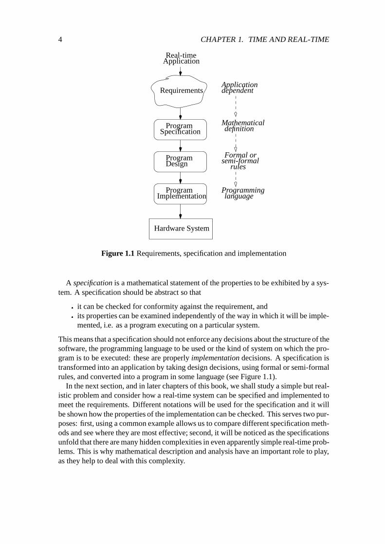
Figure 1.1 Requirements, specification and implementation
A specification is a mathematical statement of the properties to be exhibited by a sys-tem. A specification should be abstract so that
� it can be checked for conformity against the requirement, and� its properties can be examined independently of the way in which it will be imple-
mented, i.e. as a program executing on a particular system.
This means that a specification should not enforce any decisions about the structure of thesoftware, the programming language to be used or the kind of system on which the pro-gram is to be executed: these are properly implementation decisions. A specification istransformed into an application by taking design decisions, using formal or semi-formalrules, and converted into a program in some language (see Figure 1.1).
In the next section, and in later chapters of this book, we shall study a simple but real-istic problem and consider how a real-time system can be specified and implemented tomeet the requirements. Different notations will be used for the specification and it willbe shown how the properties of the implementation can be checked. This serves two pur-poses: first, using a common example allows us to compare different specification meth-ods and see where they are most effective; second, it will be noticed as the specificationsunfold that there are many hidden complexities in even apparently simple real-time prob-lems. This is why mathematical description and analysis have an important role to play,as they help to deal with this complexity.
1.3. THE MINE PUMP 5
������
������
�����
�����
���
���
�����������
�����������
AB
C
ED
Pump Controller
Pump
Sump
Log
Operator
HighwatersensorAirflowsensorMethanesensor
Lowwatersensor
CarbonMonoxidesensorABCDE
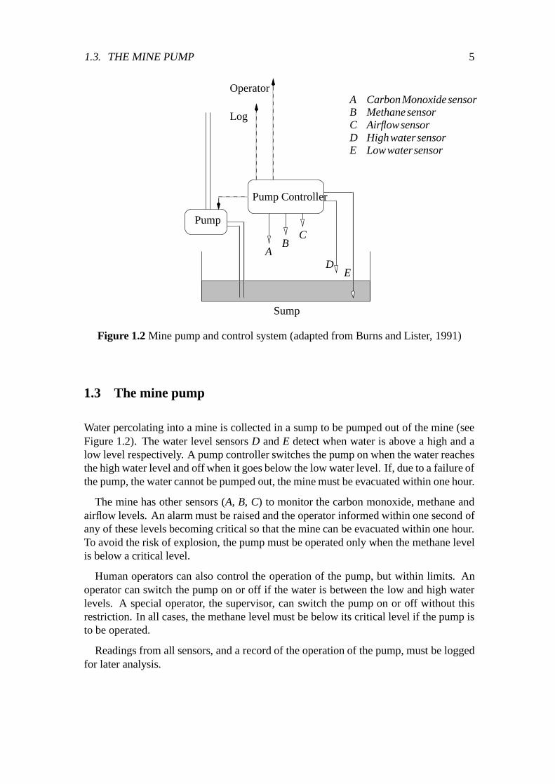
Figure 1.2 Mine pump and control system (adapted from Burns and Lister, 1991)
1.3 The mine pump
Water percolating into a mine is collected in a sump to be pumped out of the mine (seeFigure 1.2). The water level sensors D and E detect when water is above a high and alow level respectively. A pump controller switches the pump on when the water reachesthe high water level and off when it goes below the low water level. If, due to a failure ofthe pump, the water cannot be pumped out, the mine must be evacuated within one hour.
The mine has other sensors (A, B, C) to monitor the carbon monoxide, methane andairflow levels. An alarm must be raised and the operator informed within one second ofany of these levels becoming critical so that the mine can be evacuated within one hour.To avoid the risk of explosion, the pump must be operated only when the methane levelis below a critical level.
Human operators can also control the operation of the pump, but within limits. Anoperator can switch the pump on or off if the water is between the low and high waterlevels. A special operator, the supervisor, can switch the pump on or off without thisrestriction. In all cases, the methane level must be below its critical level if the pump isto be operated.
Readings from all sensors, and a record of the operation of the pump, must be loggedfor later analysis.
6 CHAPTER 1. TIME AND REAL-TIME
Safety requirementsFrom the informal description of the mine pump and its operations we obtain the follow-ing safety requirements:
1. The pump must not be operated if the methane level is critical.2. The mine must be evacuated within one hour of the pump failing.3. Alarms must be raised if the methane level, the carbon monoxide level or the air-
flow level is critical.
Operational requirementThe mine is normally operated for three shifts a day, and the objective is for no more thanone shift in 1000 to be lost due to high water levels.
ProblemWrite and verify a specification for the mine pump controller under which it can be shownthat the mine is operated whenever possible without violating the safety requirements.
CommentsThe specification is to be the conjunction of two conditions: the mine must be operatedwhen possible, and the safety requirements must not be violated. If the specification read‘The mine must not be operated when the safety requirements are violated’, then it couldbe trivially satisfied by not operating the mine at all! The specification must obviate thiseasy solution by requiring the mine to be operated when it is safely possible.
Note that the situation may not always be clearly defined and there may be times whenit is difficult to determine whether operating the mine would violate the safety require-ments. For example, the pump may fail when the water is at any level; does the timeof one hour for the evacuation of the mine apply to all possible water levels? More cru-cially, how is pump failure detected? Is pump failure always complete or can a pump failpartially and be able to displace only part of its normal output?
It is also important to consider under what conditions such a specification will be valid.If the methane or carbon monoxide levels can rise at an arbitrarily fast rate, there may notbe time to evacuate the mine, or to switch off the pump. Unless there are bounds on therate of change of different conditions, it will not be possible for the mine to be operatedand meet the safety requirements. Sensors operate by sampling at periodic intervals andthe pump will take some time to start and to stop. So the rate of change of a level mustbe small enough for conditions not to become dangerous during the reaction time of theequipment.
The control system obtains information about the level of water from the Highwaterand Lowwater sensors and of methane from the Methane sensor. Detailed data is neededabout the rate at which water can enter the mine, and the frequency and duration of met-hane leaks; the correctness of the control software is predicated on the accuracy of thisinformation. Can it also be assumed that the sensors always work correctly?
The description explains conditions under which the mine must be evacuated but doesnot indicate how often this may occur or how normal operation is resumed after an evac-

1.3. THE MINE PUMP 7
uation. For example, can a mine be evacuated more than once in a shift or, following anevacuation, is the shift considered to be lost? If the mine is evacuated, it would be normalfor a safety procedure to come into effect and for automatic and manual clearance to beneeded before operation of the mine can resume. This information will make it possibleto decide on how and when an alarm is reset once it has been raised.
1.3.1 Developing a specification
The first task in developing a specification is to make the informal description more pre-cise. Some requirements may be very well defined but it is quite common for many re-quirements to be stated incompletely or with inconsistencies between requirements. Forexample, we have seen that there may be conditions under which it is not possible to meetboth the safety requirements and the operational requirement; unfortunately, the descrip-tion gives us no guidance about what should be done in this case. In practice, it is thennecessary to go back to the user or the application engineer to ask for a more precise def-inition of the needs and to resolve inconsistencies. The process of converting informallystated requirements into a more precise form helps to uncover inconsistencies and inad-equacies in the description, and developing a specification often needs many iterations.
We shall start by trying to describe the requirements in terms of some properties, usinga simple mathematical notation. This is a first step towards making a formal specificationand we shall see various different, more complete, specifications of the problem in laterchapters.
Properties will be defined with simple predicate calculus expressions using the logicaloperators ^ (and), _ (or), ) (implies) and , (iff), and the universal quantifier 8 (forall). The usual mathematical relational operators will be used and functions, constantsand variables will be typed. We use
F : T1! T2
for a function F from type T1 (the domain of the function) to type T2 (the range of thefunction) and a variable V of type T will be defined as V : T. An interval from C1 toC2 will be represented as [C1;C2] if the interval is closed and includes both C1 and C2,as (C1;C2] if the interval is half-open and includes C2 and not C1 and as [C1;C2) if theinterval is half-open and includes C1 and not C2.
Assume that time is measured in seconds and recorded as a value in the set Time andthe depth of the water is measured in metres and is a value in the set Depth; Time andDepth are the set of real numbers.
S1: Water levelThe depth of the water in the sump depends on the rate at which water enters and leavesthe sump and this will change over time. Let us define the water level Water at any timeto be a function from Time to Depth:
Water : Time! Depth
8 CHAPTER 1. TIME AND REAL-TIME
Let Flow be the rate of change of the depth of water measured in metres per second andbe represented by the real numbers; WaterIn and WaterOut are the rates at which waterenters and leaves the sump and, since these rates can change, they are functions fromTime to Flow:
WaterIn;WaterOut : Time! Flow
The depth of water in the sump at time t2 is the sum of the depth of water at an earliertime t1 and the difference between the amount of water that flows in and out in the timeinterval [t1; t2]. Thus 8t1; t2 : Time �
Water(t2) = Water(t1)+Z t2
t1(WaterIn(t)�WaterOut(t)) dt
HighWater and LowWater are constants representing the positions of the high and lowwater level sensors. For safe operation, the pump should be switched on when the waterreaches the level HighWater and the level of water should always be kept below the levelDangerWater:
DangerWater > HighWater > LowWater
If HighWater = LowWater, the high and low water sensors would effectively be reducedto one sensor.
S2: Methane levelThe presence of methane is measured in units of pascals and recorded as a value of typePressure (a real number). There is a critical level, DangerMethane, above which thepresence of methane is dangerous.
The methane level is related to the flow of methane in and out of the mine. As forthe water level, we define a function Methane for the methane level at any time and thefunctions MethaneIn and MethaneOut for the flow of methane in and out of the mine:
Methane : Time! PressureMethaneIn;MethaneOut : Time! Pressure
and 8 t1; t2 : Time �
Methane(t2) = Methane(t1)+Z t2
t1(MethaneIn(t)�MethaneOut(t))dt
S3: Assumptions1. There is a maximum rate MaxWaterIn : Flow at which the water level in the sump
can increase and at any time t, WaterIn(t) �MaxWaterIn.2. The pump can remove water with a rate of at least PumpRating : Flow, and this
must be greater than the maximum rate at which water can build up: MaxWaterIn< PumpRating.

1.3. THE MINE PUMP 9
3. The operation of the pump is represented by a predicate on Time which indicateswhen the pump is operating:
Pumping : Time! Bool
and at any time t if the pump is operating it will produce an outflow of water of atleast PumpRating:
(Pumping(t)^Water(t) > 0))WaterOut(t) > PumpRating
4. The maximum rate at which methane can enter the mine is MaxMethaneRate. Ifthe methane sensor measures the methane level periodically every tM units of time,and if the time for the pump to switch on or off is tP, then the reaction time tM+ tPmust be such that normally, at any time t,
(Methane(t)+MaxMethaneRate � (tM + tP)+MethaneMargin)6DangerMethane
where MethaneMargin is a safety limit.5. The methane level does not reach DangerMethane more than once in 1000 shifts;
without this limit, it is not possible to meet the operational requirement. Methaneis generated naturally during mining and is removed by ensuring a sufficient flowof fresh air, so this limit has some implications for the air circulation system.
S4: Pump controllerThe pump controller must ensure that, under the assumptions, the operation of the pumpwill keep the water level within limits. At all times when the water level is high and themethane level is not critical, the pump is switched on, and if the methane level is criticalthe pump is switched off. Ignoring the reaction times, this can be specified as follows:
8t 2 Time � (Water(t) > HighWater^Methane(t) < DangerMethane)) Pumping(t)^ (Methane(t) �DangerMethane)):Pumping(t)
Now let us see how reaction times can be taken into account. Since tP is the time takento switch the pump on, a properly operating controller must ensure that
8t 2 Time �Methane(t) <DangerMethane^:Pumping(t)^Water(t) > HighWater) Pumping(t+ tP)
So if the operator has not already switched the pump on, the pump controller must do sowhen the water level reaches HighWater.
Similarly, the methane sensor may take tM units of time to detect a methane level andthe pump controller must ensure that
8t 2 Time �Pumping(t)^ (Methane(t)+MethaneMargin) =DangerMethane):Pumping(t+ tM + tP)
10 CHAPTER 1. TIME AND REAL-TIME
S5: SensorsThe high water sensor provides information about the height of the water at time t inthe form of predicates HW(t) and LW(t) which are true when the water level is aboveHighWater and LowWater respectively. We assume that at all times a correctly workingsensor gives some reading (i.e. HW(t) _:HW(t)) and, since HighWater > LowWater,HW(t)) LW(t).
The readings provided by the sensors are related to the actual water level in the sump:
8t 2 Time � Water(t) > HighWater,HW(t)^ Water(t) > LowWater , LW(t)
Similarly, the methane level sensor reads either DML(t) or :DML(t):
8t 2 Time � Methane(t) > DangerMethane, DML(t)^Methane(t) < DangerMethane,:DML(t)
S6: ActuatorsThe pump is switched on and off by an actuator which receives signals from the pumpcontroller. Once these signals are sent, the pump controller assumes that the pump actsaccordingly. To validate this assumption, another condition is set by the operation of thepump. The outflow of water from the pump sets the condition PumpOn; similarly, whenthere is no outflow, the condition is PumpOff .
The assumption that the pump really is pumping when it is on and is not pumping whenit is off is specified below:
8t 2 Time � PumpOn(t) ) Pumping(t)^PumpOff (t)):Pumping(t)
The condition PumpOn is set by the actual outflow and there may be a delay before theoutflow changes when the pump is switched on or off. If there were no delay, the impli-cation) could be replaced by the two-way implication iff, represented by ,, and thetwo conditions PumpOn and PumpOff could be replaced by a single condition.
1.3.2 Constructing the specification
The simple mathematical notation used so far provides a more abstract and a more precisedescription of the requirements than does the textual description. Having come so far,the next step should be to combine the definitions given in S1–S6 and use this to provethe safety properties of the system. The combined definition should also be suitable fortransformation into a program specification which can be used to develop a program.
Unfortunately, this is where the simplicity of the notation is a limitation. The defini-tions S1–S6 can of course be made more detailed and perhaps taken a little further to-wards what could be a program specification. But the mathematical set theory used forthe specification is both too rich and too complex to be useful in supporting program de-velopment. To develop a program, we need to consider several levels of specification

1.4. HOW TO READ THE BOOK 11
(and so far we have just outlined the beginnings of one level) and each level must beshown to preserve the properties of the previous levels. The later levels must lead di-rectly to a program and an implementation and there is nothing so far in the notation tosuggest how this can be done.
What we need is a specification notation that has an underlying computational modelwhich holds for all levels of specification. The notation must have a calculus or a proofsystem for reasoning about specifications and a method for transforming specifications toprograms. That is what we shall seek to accomplish in the rest of the book. Chapters 5–7contain different formal notations for specifying and reasoning about real-time programs;in Chapter 8 this is extended to consider the requirements of fault-tolerance in the minepump system. Each notation has a precisely defined computational model, or semantics,and rules for transforming specifications into programs.
1.3.3 Analysis and implementation
The development of a real-time program takes us part of the way towards an implemen-tation. The next step is to analyze the timing properties of the program and, given thetiming characteristics of the hardware system, to show that the implementation of theprogram will meet the timing constraints. It is not difficult to understand that for mosttime-critical systems, the speed of the processor is of great importance. But how exactlyis processing speed related to the statements of the program and to timing deadlines?
A real-time system will usually have to meet many demands within limited time. Theimportance of the demands may vary with their nature (e.g. a safety-related demand maybe more important than a simple data-logging demand) or with the time available for aresponse. So the allocation of the resources of the system needs to be planned so thatall demands are met by the time of their deadlines. This is usually done using a sched-uler which implements a scheduling policy that determines how the resources of the sys-tem are allocated to the program. Scheduling policies can be analyzed mathematicallyso the precision of the formal specification and program development stages can be com-plemented by a mathematical timing analysis of the program properties. Taken together,specification, verification and timing analysis can provide accurate timing predictions fora real-time system.
Scheduling analysis is described in Chapters 2–4; in Chapter 3 it is used to analyze anAda 95 program for the mine pump controller.
1.4 How to read the book
The remaining chapters of this book are broadly divided into two areas: (a) schedulingtheory and (b) the specification and verification of real-time and fault-tolerant propertiesof systems. The book is organized so that an interested reader can read chapters in theorder in which they appear and obtain a good understanding of the different methods. The

12 CHAPTER 1. TIME AND REAL-TIME
fact that each chapter has a different author should not cause any difficulties as chaptershave a very similar structure, follow a common style and have cross-references.
Readers with more specialized interests may wish to focus attention on just some ofthe chapters and there are different ways in which this may be done:
� Scheduling theory: Chapters 2, 3 and 4 describe different aspects of the applica-tion of scheduling theory to real-time systems. Chapter 2 has introductory ma-terial which should be readily accessible to all readers and Chapter 3 follows onwith more advanced material and shows how a mine pump controller can be pro-grammed in Ada 95; these chapters are concerned with methods of analysis forfixed priority scheduling. Chapter 4 introduces dynamic priority scheduling andshows how this method can be used effectively when the future load of the systemcannot be calculated in advance.
� Scheduling and specification: Chapters 2, 3 and 4 provide a compact overview offixed and dynamic priority scheduling. Chapters 5, 6 and 7 are devoted to specifi-cation and verification using assertional methods, a real-time process calculus andthe duration calculus respectively; one or more of these chapters can therefore bestudied to understand the role of specification in dealing with complex real-timeproblems.
� Specification and verification: any or all of Chapters 5, 6 and 7 can be used; if achoice must be made, then using either Chapters 5 and 6, or Chapters 5 and 7, willgive a good indication of the range of methods available.
� Timing and fault-tolerance: Chapter 8 shows how reasoning about fault-tolerancecan be done at the specification level; it assumes that the reader has understoodChapter 5 as it uses very similar methods.
� The mine pump: Different treatments of the mine pump problem can be found inChapters 1, 3, 5, 6, 7 and 8; though they are based on the description in this chap-ter, subtle differences may arise from the nature of the method used, and these arepointed out.
Each chapter has a section describing the historical background to the work and anextensive bibliography is provided at the end of the book to allow the interested readerto refer to the original sources and obtain more detail.
Examples are included in most chapters, as well as a set of exercises at the end of eachchapter. The exercises are all drawn from the material contained in the chapter and rangefrom easy to relatively hard.
1.5 Historical background
Operations research has been concerned with problems of job sequencing, timing, sched-uling and optimization for many decades. Techniques from operations research provided
1.5. HISTORICAL BACKGROUND 13
the basis for the scheduling analysis of real-time systems and the paper by Liu and Lay-land (1973) remained influential for well over a decade. This was also the time of the de-velopment of axiomatic proof techniques for programming languages, starting with theclassic paper by Hoare (1969). But the early methods for proving the correctness of pro-grams were concerned only with their ‘functional’ properties and Wirth (1977) pointedout the need to distinguish between this kind of program correctness and the satisfac-tion of timing requirements; axiomatic proof methods were forerunners of the assertionalmethod described and used in Chapters 5 and 8. Mok (1983) pointed out the difficulties inrelating work in scheduling theory with assertional methods and with the needs of prac-tical, multi-process programming; it is only recently that some progress has been madein this direction: e.g. see Section 5.7.1 and Liu et al. (1995).
There are many ways in which the timing properties of programs can be specified andverified. The methods can be broadly divided into three classes.
1. Real-time without time: Observable time in a program’s execution can differ to anarbitrary extent from universal or absolute time and Turski (1988) has argued that timeis an issue to be considered at the implementation stage but not in a specification; Hehner(1989) shows how values of time can be used in assertions and for reasoning about simpleprogramming constructs, but also recommends that where there are timing constraints itis better to construct a program with the required timing properties than to try to computethe timing properties of an arbitrary program. For programs that can be implemented withfixed schedules on a single processor, or those with very restricted timing requirements,these restrictions make it possible to reason about real-time programs without reasoningabout time.
2. Synchronous real-time languages: The synchrony hypothesis assumes that externalevents are ordered in time and the program responds as if instantaneously to each event.The synchrony hypothesis has been used in the ESTEREL (Berry & Gonthier, 1992), LUS-TRE and SIGNAL family of languages, and in Statecharts (Harel, 1987). Treating a re-sponse as ‘instantaneous’ is an idealization that applies when the time of response issmaller than the minimum time between external events. External time is given a discreterepresentation (e.g. the natural numbers) and internal actions are deterministic and or-dered. Synchronous systems are most easily implemented on a single processor. Strongsynchrony is a more general form of synchrony applicable to distributed systems wherenondeterminism is permitted but events can be ordered by a global clock.
3. Asynchronous real-time: In an asynchronous system, external events occur at timesthat are usually represented by a dense domain (such as the real numbers), and the systemis expected to provide responses within time-bounds. This is the most general model ofreal-time systems and is applicable to single-processor, multi-processor and distributedsystems. With some variations, this is the model we shall use for much of this book. Aswe shall see, restrictions must be imposed (or further assumptions made) to enable thetiming properties of an asynchronous model to be fully determined: e.g. using discreterather than dense time, imposing determinism, and approximating cyclic behaviour andaperiodicity by periodic behaviours. Few of these restrictions are really compatible with

14 CHAPTER 1. TIME AND REAL-TIME
the asynchrony model but they can be justified because without them analysis of the tim-ing behaviour may not be possible.
The mine pump problem was first presented by Kramer et al. (1983) and used by Burnsand Lister (1991) as part of the description of a framework for developing safety-criticalsystems. A more formal account of the mine pump problem was given by Mahony andHayes (1992) using an extension of the Z notation. The description of the mine pump inthis chapter has made extensive use of the last two papers, though the alert reader will no-tice some changes. The first descriptions of the mine pump problem, and the descriptiongiven here, assume that the requirements are correct and that the only safety considera-tions are those that follow from the stated requirements. The requirements for a practicalmine pump system would need far more rigorous analysis to identify hazards and checkon safety conditions under all possible operating conditions (see e.g. Leveson, 1995).Use of the methods described in this book would then complement this analysis by pro-viding ways of checking the specification, the program and the timing of the system.
1.6 Exercises
Exercise 1.1 Define the condition Alarm which must be set when the water, methane orairflow levels are critical. Recall that, according to the requirements, Alarm must be setwithin one second of a level becoming critical. Choose an appropriate condition underwhich Alarm can be reset to permit safe operation of the mine to be resumed.
Exercise 1.2 Define the condition Operator under which the human operator can switchthe pump on or off. Define a similar condition Supervisor for the supervisor and describewhere the two conditions differ.
Exercise 1.3 In S4, separate definitions are given for the operation of the pump con-troller and for the delays, tP to switch the pump on and tM for the methane detector. Con-struct a single definition for the operation of the pump taking both these delays into ac-count.
Exercise 1.4 Suppose there is just one water level sensor SW. What changes will needto be made in the definitions in S1 and S5? (N.B.: in Chapter 7 it is assumed that thereis one water level sensor.)
Exercise 1.5 Suppose a methane sensor can fail and that following a failure, a sensordoes not resume normal operation. Assume that it is possible to detect this failure. Tocontinue to detect methane levels reliably, let three sensors DML1, DML2 and DML3 beused and assume that at most one sensor can fail. If the predicate MOKi is true when theith methane sensor is correct, i.e. operating according to the definition in S6, and falseif the sensor has failed, define a condition which guarantees that the methane level sen-sor reading DML is always correct. (Hint: Since at most one sensor can fail, the correctreading is the same as the reading of any two equal sensor readings. N.B.: Chapter 8examines the reliability of the mine pump controller in greater detail.)

Chapter 2
Fixed Priority Scheduling – A SimpleModel
Mathai Joseph
Introduction
Consider a simple, real-time program which periodically receives inputs from a deviceevery T units of time, computes a result and sends it to another device. Assume that thereis a deadline of D time units between the arrival of an input and the despatch of the cor-responding output.
For the program to meet this deadline, the computation of the result must take alwaysplace in less than D time units: in other words, for every possible execution path throughthe program, the time taken for the execution of the section of code between the inputand output statements must be less than D time units.
If that section of the program consists solely of assignment statements, it would bepossible to obtain a very accurate estimate of its execution time as there will be just onepath between the statements. In general, however, a program will have a control structurewith several possible execution paths.
For example, consider the following structured if statement:
1 Sensor_Input.Read(Reading);2 if Reading = 5 then Sensor_Output.Write(20)3 elseif Reading < 10 then Sensor_Output.Write(25)4 else ...5 Sensor_Output.Write( ...)6 end if;
There are a number of possible execution paths through this statement: e.g. there isone path through lines 1, 2 and 6 and another through lines 1, 2, 3 and 6. Paths willgenerally differ in the number of boolean tests and assignment statements executed andso, on most computers, will take different execution times.
In some cases, as in the previous example, the execution time of each path can be com-puted statically, possibly even by a compiler. But there are statements where this is not
15
16 CHAPTER 2. FIXED PRIORITY SCHEDULING – A SIMPLE MODEL
possible:
Sensor_Input.Read(Reading);while X > Reading + Y loop
...end
Finding all the possible paths through this statement may not be easy: even if it isknown that there are m different paths for any one iteration of this while loop, the ac-tual number of iterations will depend on the input value in Reading. But if the range ofpossible input values is known, it may then be possible to find the total number of pathsthrough the loop. Since we are concerned with real-time programs, let us assume that theprogram has been constructed so that all such loops will terminate and therefore that thenumber of paths is finite.
So, after a simple examination of alternative and iterative statements, we can concludethat:
� it is not possible to know in advance exactly how long a program execution willtake, but
� it may be possible to find the range of possible values of the execution time.
Rather than deal with all possible execution times, one solution is to use just the longestpossible, or worst-case, execution time for the program. If the program will meet itsdeadline for this worst-case execution, it will meet the deadline for any execution.
Worst-caseAssume that the worst-case upper bound to the execution time can be computed for anyreal-time program.
2.1 Computational model
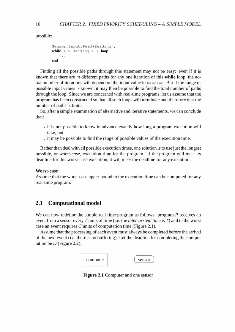
We can now redefine the simple real-time program as follows: program P receives anevent from a sensor every T units of time (i.e. the inter-arrival time is T) and in the worstcase an event requires C units of computation time (Figure 2.1).
Assume that the processing of each event must always be completed before the arrivalof the next event (i.e. there is no buffering). Let the deadline for completing the compu-tation be D (Figure 2.2).
computer sensor
Figure 2.1 Computer and one sensor

2.1. COMPUTATIONAL MODEL 17
TT
C
inputs
time
Figure 2.2 Timing diagram 1
If D < C, the deadline cannot be met. If T < D, the program must still process eachevent in a time � T if no events are to be lost. Thus the deadline is effectively boundedby T and we need to handle only those cases where
C � D � T
Now consider a program which receives events from two sensors (Figure 2.3). Inputsfrom Sensor 1 come every T1 time units and each needs C1 time units for computation;events from Sensor 2 come every T2 time units and each needs C2 time units. Assumethe deadlines are the same as the periods, i.e. T1 time units for Sensor 1 and T2 time unitsfor Sensor 2. Under what conditions will these deadlines be met?
More generally, if a program receives events from n such devices, how can it be de-termined if the deadline for each device will be satisfied?
Before we begin to analyze this problem, we first define a program model and a sys-tem model. This allows us to study the problem of timing analysis in a limited context.We consider simple models in this chapter; more elaborate models will be considered inChapters 3 and 4.
Program modelAssume that a real-time program consists of a number of independent tasks that do notshare data or communicate with each other. A task is periodically invoked by the occur-rence of a particular event.
�� ��
4T13T12T1
T2 2T2
sensor 1
sensor 2
T1
Figure 2.3 Timing diagram 2

18 CHAPTER 2. FIXED PRIORITY SCHEDULING – A SIMPLE MODEL
System modelAssume that the system has one processor; the system periodically receives events fromthe external environment and these are not buffered. Each event is an invocation for aparticular task. Note that events may be periodically produced by the environment orthe system may have a timer that periodically creates the events.
Let the tasks of program P be τ1; τ2; : : : ; τn. Let the inter-arrival time, or period, forinvocations to task τi be Ti and let the computation time for each such invocation be Ci.
We shall use the following terminology:
� A task is released when it has a waiting invocation.
� A task is ready as long as the processing associated with an invocation has not beencompleted.
� A processor is idle when it is not executing a task.
2.2 Static scheduling
One way to schedule the program is to analyze its tasks statically and determine theirtiming properties. These times can be used to create a fixed scheduling table accordingto which tasks will be despatched for execution at run-time. Thus, the order of executionof tasks is fixed and it is assumed that their execution times are also fixed.
Typically, if tasks τ1; τ2; : : : ; τn have periods of T1; T2; : : : ; Tn, the table must coverscheduling for a length of time equal to the least common multiple of the periods, i.e.LCM(fT1; T2; : : : ; Tng), as that is the time in which each task will have an integral num-ber of invocations. If any of the Ti are co-primes, this length of time can be extremelylarge so where possible it is advisable to choose values of Ti that are small multiples ofa common value.
Static scheduling has the significant advantage that the order of execution of tasks isdetermined ‘off-line’, before the execution of the program, so the run-time schedulingoverheads can be very small. But it has some major disadvantages:
� There is no flexibility at run-time as all choices must be made in advance and musttherefore be made conservatively to cater for every possible demand for computa-tion.
� It is difficult to cater for sporadic tasks which may occur occasionally, if ever, butwhich have high urgency when they do occur.
For example, an alarm condition which requires a system to be shut down within a shortinterval of time may not occur very often but its task must still be accommodated in thescheduling table so that its deadline will be met if the alarm condition does occur.

2.3. SCHEDULING WITH PRIORITIES 19
��
overrunhere
τ1
τ2
τ3
2 7 14
6 16
0 13time
Figure 2.4 Priorities without pre-emption
2.3 Scheduling with priorities
In scheduling terms, a priority is usually a positive integer representing the urgency orimportance assigned to an activity. By convention, the urgency is in inverse order tothe numeric value of the priority and priority 1 is the highest level of priority. We shallassume here that a task has a single, fixed priority. Consider the following two simplescheduling disciplines:
Priority-based executionWhen the processor is idle, the ready task with the highest priority is chosen for execu-tion; once chosen, a task is run to completion.
Pre-emptive priority-based executionWhen the processor is idle, the ready task with the highest priority is chosen for execu-tion; at any time execution of a task can be pre-empted if a task of higher priority becomesready. Thus, at all times the processor is either idle or executing the ready task with thehighest priority.
Example 2.1 Consider a program with 3 tasks, τ1, τ2 and τ3, that have the priorities,repetition periods and computation times defined in Figure 2.4. Let the deadline Di foreach task τi be Ti. Assume that the tasks are scheduled according to priorities, with nopre-emption.
Priority Period Comp.timeτ1 1 7 2τ2 2 16 4τ3 3 31 7
If all three tasks have invocations and are ready at time=0, task τ1 will be chosen forexecution as it has the highest priority. When it has completed its execution, task τ2 willbe executed until its completion at time=6.

20 CHAPTER 2. FIXED PRIORITY SCHEDULING – A SIMPLE MODEL
��
9
τ1
τ2
τ3
2 7 14
6 20
0 21time
Figure 2.5 Priorities with pre-emption
At that time, only task τ3 is ready for execution and it will execute from time=6 totime=13, even though an invocation comes for task τ1 at time=7. So there is just oneunit of time for task τ1 to complete its computation requirement of two units and its nextinvocation will arrive before processing of the previous invocation is complete.
In some cases, the priorities allotted to tasks can be used to solve such problems; inthis case, there is no allocation of priorities to tasks under which task τ1 will meet itsdeadlines. But a simple examination of the timing diagram shows that between time=15and time=31 (at which the next invocation for task τ3 will arrive) the processor is notalways busy and task τ3 does not need to complete its execution until time=31. If therewere some way of making the processor available to tasks τ1 and τ2 when needed andthen returning it to task τ3, they could all meet their deadlines.
This can be done using priorities with pre-emption: execution of task τ3 will then bepre-empted at time=7, allowing task τ1 to complete its execution at time=9 (Figure 2.5).Process τ3 is pre-empted once more by task τ1 at time=14 and this is followed by thenext execution of task τ2 from time=16 to time=20 before task τ3 completes the rest ofits execution at time=21.
2.4 Simple methods of analysis
Timing diagrams provide a good way to visualize and even to calculate the timing prop-erties of simple programs. But they have obvious limits, not least of which is that a verylong sheet of paper might be needed to draw some timing diagrams! A better method ofanalysis would be to derive conditions to be satisfied by the timing properties of a pro-gram for it to meet its deadlines.
Let an implementation consist of a hardware platform and the scheduler under whichthe program is executed. An implementation is called feasible if every execution of theprogram will meet all its deadlines.

2.4. SIMPLE METHODS OF ANALYSIS 21
Using the notation of the previous section, in the following sections we shall considera number of conditions that might be applied. We shall first examine conditions that arenecessary to ensure that an implementation is feasible. The aim is to find necessary con-ditions that are also sufficient, so that if they are satisfied an implementation is guaranteedto be feasible.
2.4.1 Necessary conditions
Condition C18i �Ci < Ti
It is obviously necessary that the computation time for a task is smaller than its period,as, without this condition, its implementation can be trivially shown to be infeasible.
However, this condition is not sufficient, as can be seen from the following example.
Example 2.2
Priority Period Comp.timeτ1 1 10 8τ2 2 5 3
At time=0, execution of task τ1 begins (since it has the higher priority) and this willcontinue for eight time units before the processor is relinquished; task τ2 will thereforemiss its first deadline at time=5.
Thus, under Condition C1, it is possible that the total time needed for computation inan interval of time is larger than the length of the interval. The next condition seeks toremove this weakness.
Condition C2i
∑j=1
�Cj=Tj
� � 1
Ci=Ti is the utilization of the processor in unit time at level i. Condition C2 improves onCondition C1 in an important way: not only is the utilization Ci=Ti required to be lessthan 1 but the sum of this ratio over all tasks is also required not to exceed 1. Thus, takenover a sufficiently long interval, the total time needed for computation must lie withinthat interval.
This condition is necessary but it is not sufficient. The following example shows animplementation which satisfies Condition C2 but is infeasible.

22 CHAPTER 2. FIXED PRIORITY SCHEDULING – A SIMPLE MODEL
Example 2.3
Priority Period Comp.timeτ1 1 6 3τ2 1 9 2τ3 2 11 2
Exercise 2.4.1 Draw a timing diagram for Example 2.3 and show that the deadline forτ3 is not met.
Condition C2 checks that over an interval of time the arithmetic sum of the utilizationsCi=Ti is � 1. But that is not sufficient to ensure that the total computation time neededfor each task, and for all those of higher priority, is also smaller than the period of eachtask.
Condition C3
8i �i�1
∑j=1
�Ti
Tj�Cj
�� Ti�Ci
Here, Condition C2 has been strengthened so that, for each task, account is taken ofthe computation needs of all higher priority tasks. Assume that Ti=Tj represents integerdivision:
� Processing of all invocations at priority levels 1 : : : i�1 must be completed in thetime Ti�Ci, as this is the ‘free’ time available at that level.
� At each level j, 1� j� i�1, there will be Ti=Tj invocations in the time Ti and eachinvocation will need a computation time of Cj.
Hence, at level j the total computation time needed is
Ti
Tj�Cj
and summing this over all values of j < i will give the total computation needed at leveli. Condition C3 says that this must be true for all values of i.
This is another necessary condition. But, once again, it is not sufficient: if Tj > Ti,Condition C3 reduces to Condition C1 which has already been shown to be not sufficient.
There is another problem with Condition C3. It assumes that there are Ti=Tj invoca-tions at level j in the time Ti. If Ti is not exactly divisible by Tj, then either dTi=Tje is anoverestimate of the number of invocations or bTi=Tjc is an underestimate. In both cases,an exact condition will be hard to define.
To avoid the approximation resulting from integer division, consider an interval Miwhich is the least common multiple of all periods up to Ti:
Mi = LCM(fT1;T2; : : : ;Tig)Since Mi is exactly divisible by all Tj; j< i, the number of invocations at any level j withinMi is exactly Mi=Mj.
This leads to the next condition.

2.4. SIMPLE METHODS OF ANALYSIS 23
Condition C4i
∑j=1
�Cj�
Mi=Tj
Mi
�� 1
Condition C4 is the Load Relation and must be satisfied by any feasible implementa-tion. However, this condition averages the computational requirements over each LCMperiod and can easily be shown to be not sufficient.
Example 2.4
Priority Period Comp.timeτ1 1 12 5τ2 2 4 2
Since the computation time of task τ1 exceeds the period of task τ2, the implementationis infeasible, though it does satisfy Condition C4.
Condition C4 can, moreover, be simplified to
i
∑j=1
�Cj=Tj
� � 1
which is Condition 2 and thus is necessary but not sufficient.Condition C2 fails to take account of an important requirement of any feasible imple-
mentation. Not only must the average load be smaller than 1 over the interval Mi, but theload must at all times be sufficiently small for the deadlines to be met. More precisely,if at any time T there are t time units left for the next deadline at priority level i, the totalcomputation requirement at time T for level i and all higher levels must be smaller thant. Since it averages over the whole of the interval Mi, Condition C2 is unable to takeaccount of peaks in the computational requirements.
But while on the one hand it is necessary that at every instant there is sufficient com-putation time remaining for all deadlines to be met, it is important to remember that oncea deadline at level i has been met there is no further need to make provision for compu-tation at that level up to the end of the current period. Conditions which average over along interval may take account of computations over the whole of that interval, includ-ing the time after a deadline has been met. For example, in Figure 2.5, task τ2 has met itsfirst deadline at time=6 and the computations at level 1 from time=7 to time=9 and fromtime=14 to time=16 cannot affect τ2’s response time, even though they occur before theend of τ2’s period at time=16.
2.4.2 A sufficient condition
So far, we have assumed that priorities are assigned to tasks in some way that character-izes their urgency, but not necessarily in relation to their repetition periods (or deadlines).

24 CHAPTER 2. FIXED PRIORITY SCHEDULING – A SIMPLE MODEL
18
τ1
τ2
6 12
time
Figure 2.6 Timing diagram for Example 2.5
Consider, instead, assigning priorities to tasks in rate-monotonic order, i.e. in the inverseorder to their repetition periods. Assume that task deadlines are the same as their peri-ods. It can then be shown that if under a rate-monotonic allocation an implementation isinfeasible then it will be infeasible under all other similar allocations.
Let time=0 be a critical instant, when invocations to all tasks arrive simultaneously.For an implementation to be feasible, the following condition must hold.
Condition C5� The first deadline for every task must be met.� This will occur if the following relation is satisfied:
n�
21=n�1��
n
∑i=1
Ci=Ti
For n = 2, the upper bound to the utilization ∑ni=1 Ci=Ti is 82:84%; for large values of n
the limit is 69:31%.This bound is conservative: it is sufficient but not necessary. Consider the following
example.
Example 2.5
Priority Period Comp.timeτ1 1 6 4τ2 2 12 4
In this case (Figure 2.6), the utilisation is 100% and thus fails the test. On the otherhand, it is quite clear from the graphical analysis that the implementation is feasible asall deadlines are met.
2.5 Exact analysis
Let the worst-case response time be the maximum time between the arrival of an invo-cation and the completion of computation for that invocation. Then an implementation

2.5. EXACT ANALYSIS 25
time
Tj
t0t
j
Figure 2.7 Inputs([t; t0); j) = 5
is feasible if at each priority level i, the worst-case response time ri is less than or equalto the deadline Di. As before, we assume that the critical instant is at time=0.
If every task τj, j < i, has higher priority than τi, the worst-case response time Ri is
Ri = Ci +i�1
∑j=1d Ri
Tje�Cj
In this form, the equation is hard to solve (since Ri appears on both sides).
2.5.1 Necessary and sufficient conditions
In this section, we show how response times can be calculated in a constructive waywhich illustrates how they are related to the number of invocations in an interval andthe computation time needed for each invocation.
For the calculation, we shall make use of half-open intervals of the form [t; t0), t < t0,which contain all values from t up to, but not including, t0.
We first define a function Inputs([t; t0); j), whose value is the number of events at pri-ority level j arriving in the half-open interval of time [t; t0) (see Figure 2.7):
Inputs([t; t0); j) = dt0=Tje�dt=TjeThe computation time needed for these invocations is
Inputs([t; t0); j)�Cj
So, at level i the computation time needed for all invocations at levels higher than ican be defined by the function Comp([t; t0); i):
Comp([t; t0); i) =i�1
∑j=1
Inputs([t; t0); j)�Cj
26 CHAPTER 2. FIXED PRIORITY SCHEDULING – A SIMPLE MODEL
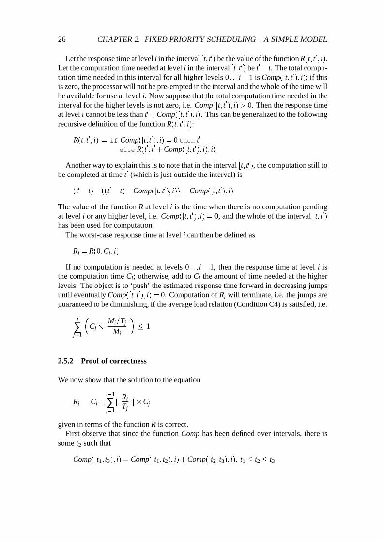
Let the response time at level i in the interval [t; t0) be the value of the function R(t; t0; i).Let the computation time needed at level i in the interval [t; t0) be t0� t. The total compu-tation time needed in this interval for all higher levels 0 : : :i�1 is Comp([t; t0); i); if thisis zero, the processor will not be pre-empted in the interval and the whole of the time willbe available for use at level i. Now suppose that the total computation time needed in theinterval for the higher levels is not zero, i.e. Comp([t; t0); i)> 0. Then the response timeat level i cannot be less than t0+Comp([t; t0); i). This can be generalized to the followingrecursive definition of the function R(t; t0; i):
R(t; t0; i) = if Comp([t; t0); i) = 0 then t0
else R(t0; t0+Comp([t; t0); i); i)
Another way to explain this is to note that in the interval [t; t0), the computation still tobe completed at time t0 (which is just outside the interval) is
(t0� t)� ((t0� t)�Comp([t; t0); i)) = Comp([t; t0); i)
The value of the function R at level i is the time when there is no computation pendingat level i or any higher level, i.e. Comp([t; t0); i) = 0, and the whole of the interval [t; t0)has been used for computation.
The worst-case response time at level i can then be defined as
Ri = R(0;Ci; i)
If no computation is needed at levels 0 : : :i� 1, then the response time at level i isthe computation time Ci; otherwise, add to Ci the amount of time needed at the higherlevels. The object is to ‘push’ the estimated response time forward in decreasing jumpsuntil eventually Comp([t; t0); i) = 0. Computation of Ri will terminate, i.e. the jumps areguaranteed to be diminishing, if the average load relation (Condition C4) is satisfied, i.e.
i
∑j=1
�Cj�
Mi=Tj
Mi
�� 1
2.5.2 Proof of correctness
We now show that the solution to the equation
Ri = Ci +i�1
∑j=1d Ri
Tje�Cj
given in terms of the function R is correct.First observe that since the function Comp has been defined over intervals, there is
some t2 such that
Comp([t1; t3); i) = Comp([t1; t2); i)+Comp([t2; t3); i); t1 � t2 � t3
2.5. EXACT ANALYSIS 27
Proof: Let the sum of the computation time needed in the interval [0; t) at the levels0 : : :i� 1 plus the time needed at level i be t0. Then an invariant INV for the recursiveequation R is
INV : Comp([0; t); i)+Ci = t0
Step 1: the initial condition R(0;Ci; i) satisfies the invariant.Step 2: by the induction hypothesis, R(t0; t0 + Comp([0; t); i); i) satisfies the invariant.Further,
Comp([0; t0); i)+Ci = t0+Comp([t; t0); i)
Since for 0� t � t0, using interval arithmetic,
Comp([0; t0); i) = Comp([0; t); i)+Comp([t; t0); i)
we can substitute and simplify this to
Comp([0; t); i)+Ci = t0
This proves the induction step.Step 3: on termination, Ri = t0 and
INV ^ Comp([t; t0); i) = 0
Substituting for INV gives
Comp([0; t0); i)+Ci = t0 ^ Ri = t0
and substituting for Comp gives i�1
∑j=1d Ri
Tje�Cj
!+Ci = t0 ^ Ri = t0
2
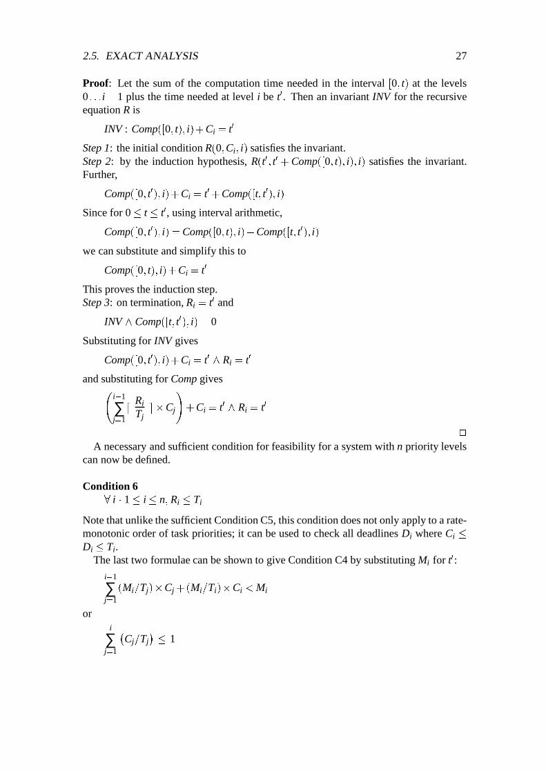
A necessary and sufficient condition for feasibility for a system with n priority levelscan now be defined.
Condition 68 i � 1� i� n; Ri � Ti
Note that unlike the sufficient Condition C5, this condition does not only apply to a rate-monotonic order of task priorities; it can be used to check all deadlines Di where Ci �Di � Ti.
The last two formulae can be shown to give Condition C4 by substituting Mi for t0:
i�1
∑j=1
(Mi=Tj)�Cj +(Mi=Ti)�Ci < Mi
ori
∑j=1
�Cj=Tj
� � 1

28 CHAPTER 2. FIXED PRIORITY SCHEDULING – A SIMPLE MODEL
2.5.3 Calculating response times
The function R can also be evaluated by rewriting it as a recurrence relation:
Rn+1i = Ci +
i�1
∑j=1d Rn
i
Tje�Cj
where Rni is the response time in the nth iteration and the required response time is the
smallest value of Rn+1i to solve this equation. In Chapter 3, the tasks τj of higher priority
than i will be collectively described by defining them as members of the set hp(i) and theequation becomes
Rn+1i = Ci + ∑
j2hp(i)
d Rni
Tje�Cj
To use the recurrence relation to find response times, it is necessary to compute Rn+1i
iteratively until the first value m is found such that Rm+1i = Rm
i ; then the response time isRm
i .Programs can be written to use either the recursive or iterative way to find response
times. In the following examples we show how response times can be found by handcalculation using the recursive definition.
Example 2.6 For the following task set, find the response time for task τ4.
Priority Period Comp.timeτ1 1 10 1τ2 2 12 2τ3 3 30 8τ4 4 600 20
Substitution shows that the task set satisfies Condition C4:
i
∑j=1
�Cj�
600=Tj
600
�� 1
The response time R4 is therefore
R(0;20;4) = if Comp([0;20);4) = 0 then20elseR(20;20+Comp([0;20);4))
Comp([0;20);4) = Inputs([0;20);1)� 1+Inputs([0;20);2)� 2+Inputs([0;20);3)� 8
=2�1+2�2+1�8=14
Repeat this calculation for R(20;34;4) by first computing

2.6. EXTENDING THE ANALYSIS 29
Comp([20;34);4)= Inputs([20;34);1)�1+Inputs([20;34);2)�2+Inputs([20;34);3)�8
=2�1+1�2+1�8=12
Calculation of the function Comp must be therefore be repeated to obtain R(34;46;4):
Comp([34;46);4)= Inputs([34;46);1)�1+Inputs([34;46);2)�2+Inputs([34;46);3)�8
=1�1+1�2=3
Comp([46;49);4)=2Comp([49;51);4)=1Comp([51;52);4)=0
Thus the response time R(0;20;4) = R(0;52;4) for task τ4 is 52.
2.6 Extending the analysis
The rate-monotonic order provides one way of assigning priorities to tasks. It is easyto think of other ways: e.g. in deadline-monotonic order (if deadlines are smaller thanperiods). Priorities can also be assigned to tasks in increasing order of slack time, wherethe slack time for task τi is the difference Ti�Ci between its period and its computationtime. All these methods of assignment are static as the priority of a task is never changedduring execution. The method of analysis described in this chapter can be used for anystatic assignment of priorities, but it does not provide a way of choosing between them.
So far, we have considered a very simple program model with independent tasks thatdo not inter-communicate. This has made it possible to schedule tasks without regard toany dependencies between them: any task with some incomplete computation is readyand it can be scheduled whenever it is ready and the processor is free. This type of modelcan be used for simple data-logging programs but most real-time programs have a morecomplex structure. If tasks can communicate with each other, using shared memory or bymessage passing, scheduling becomes far more complicated as it is not only time-driven.A task can receive a message only after the message has been sent, so a receiving taskτ2 will not be ready to be scheduled until the corresponding sending task τ1 has beenscheduled, even if τ1 is of lower priority than τ2.
When analysis shows that no allocation of priorities to tasks is feasible, it may meanthat the single available processor is not sufficient to meet the processing load. Solutionsare then either to obtain a faster processor (thereby effectively reducing the computationtime for each task) or to add one or more processors. With multiple processors, there isthe question of exactly how the processing load is divided between the processors. Whentasks are statically assigned to processors, the analysis described here can be used for

30 CHAPTER 2. FIXED PRIORITY SCHEDULING – A SIMPLE MODEL
each processor. But two difficult problems are introduced: first, to find a good assignmentof tasks to processors so that response time requirements are met, noting that finding the‘best’ assignment of tasks to processors is in general an NP-complete problem; second,to account for communication between tasks over multiple processors, and without someconstraints this can make the analysis very difficult.
In Chapter 3, we shall consider a more elaborate program model which takes task com-munication into account. And in Chapter 4, dynamic task priorities are introduced and itis seen that their use permits more flexibility and better utilization of resources.
2.7 Historical background
The problem of assigning resources to tasks is old and has been studied using the tech-niques of operations research (e.g. linear programming, dynamic programming). In thiscontext, its best-known form is job-shop scheduling, where components are processedthrough a factory floor consisting of a number of machines. Effective job-shop schedul-ing requires generating schedules to meet hard deadlines using some form of priorities.
The first important results in the scheduling of hard-real-time systems are usually at-tributed to the classic paper by Liu and Layland (1973), which considered the questionof determining feasibility for a fixed set of independent, periodic tasks and identified thecritical instant at which all tasks are ready to start computation. Their method of analysisand their proof of the optimality of the rate-monotonic order resulted in much subsequentwork being focussed on rate-monotonic scheduling (though, as we have seen here, otherfixed priority scheduling methods are also of importance).
Necessary tests (e.g. Joseph, 1985) for feasibility were replaced by necessary and suf-ficient tests, together with a proof of correctness, in Joseph and Pandya (1986) whereresponse time analysis was used to determine the feasibility of any fixed priority orderwith task deadlines Ci � Di � Ti. Harter (1987), working with a simple temporal logicproof system, studied response time analysis for a program model that allowed procedurecalls between tasks at different priority levels. Lehoczky et al. (1989) studied systemswhere Di = Ti (i.e. the Liu and Layland model) and developed a necessary and suffi-cient condition for feasibility using workloads, in terms of processor utilization; Nassorand Bres (1991) extended this to allow Di � Ti. Audsley et al. (1991) defined responsetimes using a recurrence relation, in which form it was used in other work (e.g. Audsleyet al. 1993a) and also in what is now commonly called the Rate Monotonic Book (Kleinet al., 1993). Lehoczky (1990) used workload analysis to provide two ways to deal withcases where Di > Ti, and Tindell (1993) provided a more general analysis using responsetimes.
An excellent survey of work on fixed priority scheduling appeared in Audsley et al.(1995).

2.8. EXERCISES 31
2.8 Exercises
Exercise 2.1 A real-time program has four tasks with the following characteristics:
Priority Period Comp.timeτ1 1 5 1τ2 2 15 2τ3 3 60 3τ4 4 200 7
(a) Determine using a graphical method whether the program will meet its deadlines ifscheduled according to priorities but with no pre-emption.(b) If scheduled with priorities and pre-emption, what is the response time for task τ2?
Exercise 2.2 Given the following task set with priorities assigned in rate-monotonic or-der, check that task τ3 meets its deadline of 36.
Priority Period Comp.timeτ1 1 6 2τ2 2 18 4τ3 3 36 6
Exercise 2.3 In the following task set, the response time for task τ4 is smaller than fortask τ3:
Period Comp.time Resp. limitτ1 10 1 10τ2 12 2 12τ3 40 8 40τ4 600 20 30
Choose a suitable allocation of priorities to the tasks and show that the response timelimits for all tasks can be met.
Exercise 2.4 For the following task set:
Period Comp.timeτ1 100 1τ2 10 4τ3 14 6τ4 50 8
check whether there is an assignment of priorities to tasks under which each task willmeet its deadlines.

Chapter 3
Advanced Fixed Priority Scheduling
Alan Burns and Andy Wellings
Introduction
In this chapter, we consider an extended computational model and describe some of themore advanced methods of analysis that can be used. The features of the extended modelpermit efficient resource sharing at run-time and the methods of analysis allow effectiveprediction of the worst-case timing behaviour of an application.
The resources of a system include processors and communication media; on some sys-tems there will also be disks and specialized hardware devices. Chapter 2 consideredways in which a single processor could be shared between simple processes using dif-ferent scheduling techniques. In a similar way, run-time scheduling can be used to shareother resources. There are two aspects to the use of any scheduling technique: the run-time behaviour it produces, and the methods of analysis available for predicting tim-ing properties. As before, the computational model will be defined independently ofthe scheduling technique. The model defines the real-time software structure while thescheduling technique defines how this is mapped onto the system at run-time. Not allscheduling techniques can be used if accurate predictions of the resulting timing proper-ties are needed.
3.1 Computational model
Most embedded real-time systems are inherently parallel in nature and the extended com-putational model allows the definition of concurrent tasks, each of which can be invokedrepeatedly. Tasks may be periodic or sporadic. A periodic task is released by a timerevent and a sporadic task by an event originating either from another task or from the en-vironment of the system (typically as an interrupt). In Chapter 2, we considered eventsto be unbuffered and to be lost if they were not processed in time. Here we assume in-vocation events to be persistent: a periodic task that overruns into its next release periodcan continue directly with its next invocation.
32

3.1. COMPUTATIONAL MODEL 33
Periodic and sporadic tasks have a minimal inter-arrival time T. Sporadic tasks mayalso have global constraints, such as the maximum number of invocations in a period. Forexample, a sporadic task may have an inter-arrival time of 1 ms and the restriction that nomore than four invocation events occur in any 10 ms interval. As before, we shall be con-cerned with the worst-case response time R of a task. For a given scheduling technique,R represents the predicted latest possible task completion time, relative to its invocationevent. We shall assume that the number N of tasks is fixed. In a distributed system withmany processing nodes, each task is statically allocated to one node. Tasks may commu-nicate with each other asynchronously through a protected shared object (PSO) whichensures mutual exclusion over the shared data. Tasks effectively perform atomic readand write operations on the shared object; we shall see later how this can be assured bya scheduling technique. This form of asynchronous communication ensures that a task’sbehaviour is simple (and hence predictable). Apart from waiting for access to PSOs,a task will proceed from its invocation event to the completion of that invocation in astraightforward way. The scheduling technique will ensure that tasks are blocked for theminimum time when attempting to access PSOs. A task execution must not voluntarilysuspend itself during an invocation. For example, a task which sets up an input opera-tion from an external device, and which must wait for a minimum time before reading theinput value, cannot delay itself. Instead, the operation must be implemented using twotasks with the delay represented by setting a time offset between their executions. Analternative to asynchronous communication would be to allow tasks to exchange data di-rectly, e.g. using an Ada rendezvous so that a PSO would then not be needed. As a taskcan always be used to implement a PSO, it is clear that there is no fundamental distinc-tion between the two approaches. But we shall show that asynchronous communicationallows enough flexibility in program design and permits efficient scheduling.
A software system therefore consists primarily of tasks and PSOs; like tasks, PSOsmay be distributed over the nodes of a distributed system. To deal with the typical timingrequirements of real-time systems we add the mechanism of a transaction to link inputand output activities that have associated deadlines. A transaction may be periodic, witha deadline relative to some initial timing event, or sporadic, with a deadline relative toan input event. Transactions will be used to reflect end-to-end properties, i.e. from aninput event to an output response. In a distributed system, input and output may be ondifferent nodes and an end-to-end property may therefore cross node boundaries.
3.1.1 Example of transactions
Transactions are implemented using tasks and PSOs. A simple (non-distributed) transac-tion may be implemented as a single task but, more typically, a transaction will involvea number of tasks related in some precedence order.
For example, consider a simple periodic transaction consisting of three tasks, τ1, τ2and τ3. Assume that data is processed by the tasks in the order τ1, τ2 and τ3. Let theprecedence order over the tasks be represented by the operator �.
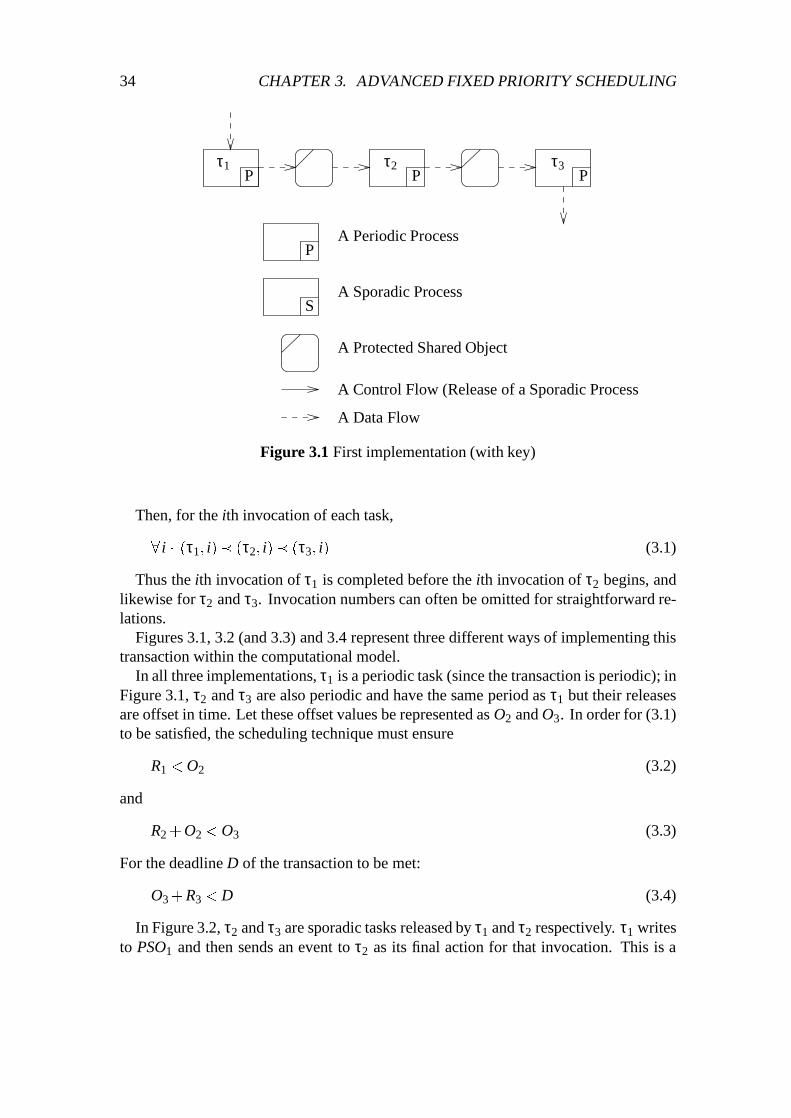
34 CHAPTER 3. ADVANCED FIXED PRIORITY SCHEDULING
P
S
A Data Flow
A Control Flow (Release of a Sporadic Process
A Protected Shared Object
A Sporadic Process
A Periodic Process
τ1P
τ2P
τ3P
Figure 3.1 First implementation (with key)
Then, for the ith invocation of each task,
8i � (τ1; i)� (τ2; i)� (τ3; i) (3.1)
Thus the ith invocation of τ1 is completed before the ith invocation of τ2 begins, andlikewise for τ2 and τ3. Invocation numbers can often be omitted for straightforward re-lations.
Figures 3.1, 3.2 (and 3.3) and 3.4 represent three different ways of implementing thistransaction within the computational model.
In all three implementations, τ1 is a periodic task (since the transaction is periodic); inFigure 3.1, τ2 and τ3 are also periodic and have the same period as τ1 but their releasesare offset in time. Let these offset values be represented as O2 and O3. In order for (3.1)to be satisfied, the scheduling technique must ensure
R1 < O2 (3.2)
and
R2 +O2 < O3 (3.3)
For the deadline D of the transaction to be met:
O3+R3 < D (3.4)
In Figure 3.2, τ2 and τ3 are sporadic tasks released by τ1 and τ2 respectively. τ1 writesto PSO1 and then sends an event to τ2 as its final action for that invocation. This is a

3.1. COMPUTATIONAL MODEL 35
P S Sτ1 τ2 τ3
PSO1 PSO2
Figure 3.2 Second implementation (showing PSOs)
P St1 t2 t3
P
Figure 3.3 Second implementation (PSOs not shown)
commonly needed pair of operations and there is therefore an advantage in combiningthem into a single operation; we shall see in Section 3.3 that this has been done in Ada 95.We shall use a combined operation in subsequent diagrams, for example by redrawingFigure 3.2 as Figure 3.3; note that the arrow denoting control flow now also implies apossible data flow.
Relation 3.1 is satisfied by definition in this second implementation. To meet the trans-action requirement, the following condition must be met:
R1 +R2+R3 < D (3.5)
The second implementation has the advantage that its overall worst-case response timeis likely to be less than that provided by the first implementation. This is because thetimer events are spread out (e.g. because the hardware platform may not be able to sup-port the release of periodic tasks at arbitrary times). Hence O2 may be somewhat largerthan R1, and the scheduling technique may be able to guarantee (3.5) but not (3.4).
There is another property of the second implementation which may, or may not, be anadvantage. Not only may the worst-case response time be less but the average- and best-case response times may also be less. Response times are calculated for the maximumload, and for certain patterns of invocation the load may be much less than the maximum.Hence, in the second implementation, data could ripple quickly through the system.
It is not always possible to guarantee that timing properties are strictly met. For exam-ple, a periodic event may in fact occur at times either a little before or a little later thanits strict period. This jitter can have many effects and certain control applications may

36 CHAPTER 3. ADVANCED FIXED PRIORITY SCHEDULING
P S Pτ1 τ2 τ3
Figure 3.4 Third implementation
become unstable if results are output too early. So, in addition to a deadline, a transac-tion may need to have a maximum output jitter defined: e.g. to produce output withinthe interval [D� J, D], where J is a jitter constant.
Assume, for illustration, that the minimum response time of all tasks is 0. Then thesecond implementation has an output bound of [0, R1 +R2 +R3], while the first imple-mentation has a much tighter bound of [O3, O3+R3] and this may make it conform moreclosely to the requirements.
The third implementation (Figure 3.4) attempts to combine the best features of the twoearlier attempts by keeping the end-to-end response time small without making the tim-ing conditions too rigid. Here τ2 is sporadic but τ3 is periodic. This implementation hasthe same bound on its output as for the second implementation (i.e. [O3, O3 +R3]) buthas a potentially lower value for O3:
R1 +R2 < O3 (3.6)
The advantages of the third implementation increase with the number of tasks in the trans-action. For example, if there are ten tasks it is still only the first and last tasks that needto be periodic.
In general, tasks may be associated with more than one transaction and the precedencerelations between tasks can include branching and joining. Even with the simple exampledescribed above, it is clear that there are a number of design choices to be made. It isthe role of a design method to provide the means by which a task set corresponding toa computational model is obtained from the system specification. Design methods willnot be considered here in detail but some references can be found in Section 3.5.
3.1.2 Allocation
To prevent a task from suspending itself while accessing PSOs, the computational modelmust impose restrictions on remote actions (i.e. actions from one processing node to an-other): a task may read or write from a local PSO, may write to a remote PSO but maynot read from a remote PSO.
To read from a remote PSO would involve suspending the task and would require theunderlying execution environment to support a remote procedure call (RPC) mechanism.Unfortunately, RPC mechanisms are not usually amenable to timing analysis because of

3.1. COMPUTATIONAL MODEL 37
R1P
P
PR2
W
Figure 3.5 Centralized readers and writer
R1
R2W
N N
P P
PP
Copy
Figure 3.6 Distributed readers and writer
the effects of the communications network and the remote processor. By restricting themodel, all that is required from the execution environment is an asynchronous messagetransfer feature that can place data in a remote PSO or release a remote sporadic task forexecution.
The disadvantage of this restriction is that it may be difficult to distribute a programacross a set of nodes. For example, to take an extreme case, if all the tasks in a programread from one PSO, they would all need to be located on the same node as the PSO. How-ever, in practice, programs are not often so centralized and simple transformations to theprogram structure can usually make distributed allocation possible.
Consider a program with one PSO that is read by two tasks (R1 and R2) that must beallocated to different nodes because they interact directly with devices on these nodes.Clearly, the PSO can only be in one place and so the program structure must be changedto use two PSOs. Then data can be copied from the original PSO to one that is local tothe task that does not have direct access. The copying can be done in a number of ways.If the two tasks are periodic, an additional periodic task can be used with a release time,period and deadline chosen so that data will appear in the second PSO in time for it to beread (locally). This transformation of the program is illustrated in Figures 3.5 and 3.6.where the outer box depicts a node boundary.
The restriction over remote access forces all significant computational events to be ex-plicitly represented in the system description. Analysis can then be applied to all the rel-evant components and the effect of the addition of a new periodic task is easily analyzed.
38 CHAPTER 3. ADVANCED FIXED PRIORITY SCHEDULING
It is not easy to analyze the timing properties of an operating system’s RPC mechanismwhich automatically generates task stubs.
3.1.3 Summary
We have informally introduced a computational model that is appropriate for resourcesharing in distributed real-time systems. The main features of this model are summarizedbelow.
Extended program model� A program consists of tasks and Protected Shared Objects (PSOs).� Tasks and PSOs may be distributed over a physical system.� The important timing properties of tasks and PSOs are known.� A task’s behaviour consists of a potentially unbounded series of invocations, each
released by an invocation event. A task must not voluntarily suspend itself duringan invocation.
� Periodic tasks are released by local timer events.� Sporadic tasks are released by events originating in either another (possibly re-
mote) task, or from the environment of the system.� PSOs provide mutually exclusive access to the data shared between tasks.� Tasks may write to any PSO, but can only read from local PSOs.� Transactions are defined using precedence relations between tasks and are used to
represent end-to-end timing properties.
3.2 Advanced scheduling analysis
In Chapter 2, the exact analysis was based on fixed priority pre-emptive scheduling andtasks were independent and periodic. Many of these restrictions will now be relaxed.
For the simple model, the timing attributes of a task consisted of its period T, its worst-case execution time C, a deadline D and its priority P. A recurrence relationship wasdefined for the worst-case response time (or completion time) R for each task, assumingthat a fixed number N of tasks were executed on the processing node. The recurrencerelation for task τi was:
Rn+1i = Ci + ∑
j2hp(i)
d Rni
Tje�Cj (3.7)
where hp(i) is the set of tasks of higher priority than τi, and R0 is given an initial value ofCi (although more efficient initial values can be found). The value R can be consideredto be a ‘computational window’ into which C must be accommodated. When Rn
i is equalto Rn+1
i , then this value is the worst-case response time, Ri, and the goal is to ensure thatthis is less than Di.

3.2. ADVANCED SCHEDULING ANALYSIS 39
We shall now generalize equation (3.7) so that it can be used for the computationalmodel described in the previous section:
� Tasks interact through PSOs (this requires the use of a ‘priority ceiling’ protocol).� Tasks may have sporadic (non-periodic) executions.� There may be jitter over the release time of a task.� Task deadlines may take any values – including D > T.� A task may have internal deadlines and external deadlines that occur before exe-
cution of the task is completed.� Task priorities should be assigned optimally (even when D > T).� Account must be taken of the execution time overheads.
Each of these issues is considered in the following sections.
3.2.1 Worst-case execution time
We have already seen that it is necessary to find the worst-case execution time of a task.In addition to processing time, it may also be necessary to estimate the time for delays incommunication and disk access.
The worst-case execution time C can be found either by measurement or by analysis.Measurement is most useful to validate figures obtained by analysis but when used on itsown it is hard to be sure when the worst-case has been observed. The difficulty in usinganalysis is that an accurate model of the processor (including caches, pipelines, memorywait states, etc.) must be available.
Techniques used for timing analysis usually require two steps: first decompose thecode of a task into a directed graph of basic blocks which represent straightline code,then use the processor model to estimate the worst-case execution time.
Once the times for all the basic blocks are known, the directed graph can be collapsed.For example, for a simple alternative statement, the two basic blocks can be reduced toa single value (i.e. the larger of the two values for the alternative blocks). Similarly,loops can be collapsed using knowledge about maximum repetition bounds. More so-phisticated graph reduction techniques can be used if sufficient semantic information isavailable. For a simple example, consider the following code:
for I in 1..10 loopif Cond then-- 100 time unit basic block
else-- 10 time unit basic block
end ifend loop
With no further information, the total timing ‘cost’ of this fragment would be 10�100+ loopoverhead, giving a total of over 1000. But static analysis of the code mayshow that Cond is only true for, at most, three iterations, leading to a less pessimistictiming cost.

40 CHAPTER 3. ADVANCED FIXED PRIORITY SCHEDULING
PSO request
task release task competion
PSO release
prio
rity
time
τ1
τ2
τ3
Figure 3.7 Execution sequence without ceiling priorities
3.2.2 Task interactions and ceiling priority algorithms
When tasks interact through PSOs, fixed priority scheduling can give rise to the phe-nomenon of priority inversion. Consider three tasks τ1, τ2 and τ3 and assume that τ1 hasthe highest priority and τ3 the lowest. Assume also that τ1 and τ3 communicate throughPSO1. However rarely τ1 and τ3 may compete for access to PSO1, there will be occasionsfor which τ3 has gained access to the shared object just as τ1 is released for execution. τ1will pre-empt τ3 because of its higher priority but it will also be blocked as τ3 has alreadyobtained exclusive access to PSO1.
This blocking is unavoidable but it is important to bound the delay and, ideally, to makeit short. If τ2 is released during the execution of τ1, then we have a situation in whichτ1 is blocked by τ3, and τ3 is pre-empted by τ2. The blocking will last for the entireexecution time of τ2. The condition under which a lower priority process is executing(i.e. τ2) when a higher priority process (i.e. τ1) is blocked is called priority inversion.This is illustrated in Figure 3.7. A scheduling technique must aim to minimize the timeduring which priority inversion occurs.
The solution is to adopt some form of priority inheritance; we describe one method inthis section and refer to others in Section 3.5.
The method considered here is known as Immediate Ceiling Priority Inheritance(ICPI). With ICPI, all PSOs are assigned a priority equal to the maximum priority of anytask that uses it. This is its ceiling priority. Whenever a task accesses a PSO, its priority

3.2. ADVANCED SCHEDULING ANALYSIS 41
τ2prio
rity
time
τ1
τ3
Figure 3.8 Execution sequence with ceiling priorities
is immediately raised to this ceiling level. Where a PSO is accessed externally (from aremote node), the priority assigned by the execution environment (the operating system)must be used and, typically, this will be higher than any local task priority.
As a task cannot be pre-empted by another task of equal or lower priority, only one taskcan ever be executing within a PSO.1 Thus mutual exclusion, the fundamental propertyof a PSO, is guaranteed for single processor systems by this inheritance protocol. In ad-dition, ICPI has another important property:
� A task may be blocked when it is released but only by a single lower priority task;once it has started executing it will not be blocked again (although it may, of course,be pre-empted by a higher priority task).
When a task is released, there may be a lower priority task currently executing with aceiling priority of equal or higher priority. When this task has left the PSO and had itspriority returned to a lower value, the released task will pre-empt it and start executing.As a task does not voluntarily suspend itself during its execution, no further lower prioritytask can gain access to any PSOs that the released task may require. Hence it proceedsthrough its execution without further blocking. This is illustrated in Figure 3.8 whichrepresents the same behaviour as Figure 3.7, but with ICPI.
1To ensure this safety property, a pre-empted task must be placed at the front of the run queue (for itsprocessor and its priority) if it must give way to a higher priority task. This ensures that it will run beforeany other task of the same priority. An alternative is to give the PSO a ceiling priority higher than anycalling task.

42 CHAPTER 3. ADVANCED FIXED PRIORITY SCHEDULING
As a task is only blocked at the beginning of its invocation it is only blocked once. Andas a task does not start executing before it is blocked, the context switching overheadsof the protocol are low. Other protocols involve executing the task, context switching tothe blocking task, executing it and then context switching back again.
The final key property of ICPI is that it ensures that use of PSOs by tasks is deadlockfree. As a task is not blocked more than once, no circular blocking dependencies canexist. It is not possible to write a program that will deadlock when executed with fixedpriorities and ICPI.
In the analysis that follows, the maximum blocking factor will be denoted by B, whichis easily calculated: it is the maximum time for which any lower priority task can executewith a ceiling priority equal to or greater than that of the task under consideration:
Bi = maxτj2lp(i)
( maxobj2pso(i)
(usage(τj;obj))) (3.8)
where lp(i) is the set of tasks with lower priority than τi, pso(i) is the set of PSOs with aceiling priority greater than or equal to the priority of τi and usage gives the worst-caseexecution time of task τj in object obj.
Recall that the only way a task can obtain a ceiling priority is to access a PSO. The basicrecurrent equation of Chapter 2 can easily be modified to include the blocking value:
Rn+1i = Bi + Ci + ∑
j2hp(i)
�Rn
i
Tj
�Cj (3.9)
Note that while interference increases as you go down the priority order, blocking doesnot: a task can be blocked at most once.
3.2.3 Sporadic tasks and release jitter
In the simple model all tasks were assumed to be periodic and to be released with perfectperiodicity: i.e. if task τi has period Ti then it was assumed to be released with exactlythat frequency. Sporadic tasks can be incorporated into the model by assuming that theyhave some minimum inter-arrival interval. However, this is not a realistic assumption.Consider a sporadic task τs that is released by a remote periodic task τp and τp � τs; e.g.the first two tasks in Figures 3.3 and 3.4 could have this relationship. The period of thefirst task is Tp and the sporadic task will have the same period, but it is incorrect to as-sume that the maximum load (or interference) that τs exerts on low priority tasks can berepresented in equations (3.7) or (3.9) as that of a periodic task with period Ts = Tp.
To understand the reason for this, consider two consecutive executions of τp. Assumethat the event that releases τs occurs at the end of the periodic task’s execution. On thefirst execution of τp, assume that the task does not complete until its latest possible time,i.e. Rp. However, on the next invocation assume there is no interference on τp so it com-pletes within Cp. As this value could be arbitrarily small, let it be equal to zero. The twoexecutions of the sporadic task are then separated not by Tp but by Tp�Rp. Figure 3.9

3.2. ADVANCED SCHEDULING ANALYSIS 43
t
completion of periodic task and release of the sporadic task
release of periodic task
time
t+15 t+20
τP
Figure 3.9 Releases of sporadic tasks
illustrates this behaviour for Tp equal to 20, Rp equal to 15 and minimum Cp equal to1 (i.e. two sporadic tasks released within six time units). Note that this phenomenon isof interest only if τp is remote as, otherwise, the variations in the release of τs could beaccounted for by the standard equations.
To represent the interference caused by sporadic tasks upon other tasks correctly, therecurrence relation must be modified. Let the maximum variation in a task’s release becalled its jitter, represented by J. (In the example above, τs has a jitter of 15.) Examina-tion of Figure 3.7 and the way the recurrence relation was derived suggests that it shouldbe changed to the following:
Rn+1i = Bi + Ci + ∑
j2hp(i)
�Rn
i + Jj
Tj
�Cj (3.10)
In general, periodic tasks do not suffer release jitter. An implementation may, however,restrict the granularity of the system timer which releases periodic tasks. In this situationa periodic task may also suffer release jitter. For example, a period of 10 with a systemgranularity of 8 will lead to a jitter value of 6, i.e. the periodic task will be released forits time=10 invocation at time=16. If response time R�i is to be measured relative to thereal release time, then the jitter value must be added to the previous response time:
R�i = Ri + Ji (3.11)
This assumes that the response time is smaller than Ti.

44 CHAPTER 3. ADVANCED FIXED PRIORITY SCHEDULING
3.2.4 Arbitrary deadlines
When Di, and hence possibly Ri, can be greater than Ti, the analysis must be changedagain. When Di � Ti, it is only necessary to consider a single release of each task. Thecritical instant, when all higher priority tasks are released at the same time, representsthe maximum interference and hence the response time following a release at the criti-cal instant must be the worst-case response time. However, when Di > Ti, a number ofreleases must be considered.
Assume that the release of a task is delayed until all previous releases of the same taskhave been completed. For each potentially overlapping release, define a separate windoww(q), where q is the serial number of the window (i.e. q = 0;1;2; :::). Equation (3.9) canthen be extended (ignoring jitter) as follows:
Rn+1i (q) = Bi + (q+1)Ci + ∑
j2hp(i)
�Rn
i (q)
Tj
�Cj (3.12)
For example, with q = 2, three releases of task τi will occur in the window. For eachvalue of q, a stable value of w(q) can be found by iteration – as in equation (3.7). Theresponse time is
Ri(q) = Rni (q) � qTi (3.13)
e.g. with q = 2 the task started 2Ti into the window and hence the response time is thesize of the window minus 2Ti.
The number of releases that need to be considered is bounded by the lowest value ofq for which the following relation is true:
Ri(q) 6 Ti (3.14)
At this point, the task completes execution before its next release and the succeeding win-dows do not overlap. The worst-case response time is then the maximum value found foreach q:
Ri = maxq=0;1;2;:::
Ri(q) (3.15)
Note that for D6 T, relation (3.14) is true for q = 0 and equations (3.12)and (3.13) canbe simplified into their original form.
To combine the use of arbitrary deadlines with the effect of release jitter, two alter-ations must be made to this analysis. First, as before, the extent of interference must beincreased if any higher priority tasks have release jitter:
Rn+1i (q) = Bi + (q+1)Ci + ∑
j2hp(i)
�Rn
i (q)+ Jj
Tj
�Cj (3.16)
The other change is in the structure of the task: if it is subject to release jitter then twoconsecutive windows will overlap if its response time plus the extent of jitter is greaterthan the period. To accommodate this, equation (3.13) must be altered:
Ri(q) = Rni (q) � qTi + Ji (3.17)

3.2. ADVANCED SCHEDULING ANALYSIS 45
a b c d
Figure 3.10 Task execution phases
3.2.5 Internal deadlines
As we shall see shortly (Section 3.2.7), it may be necessary for the model to take accountof the overheads of context switching between tasks and to ‘charge’ this to some task.With realistic (i.e. non-zero) context switch times, the ‘deadline’ may well then not be atthe end of the context switch. Moreover, the last observable event may not be at the endof the task execution and there may be a number of internal actions after the last outputevent.
Figure 3.10 gives a block representation of a task execution (excluding pre-emptionsfor higher priority tasks). Phase a is the initial context switch to begin the executionof the task, phase b is the task’s actual execution time up to the last observable event,phase c represents the internal actions of the task following the last observable eventand, finally, phase d is the cost of the context switch at the end of the task execution.The ‘real’ deadline of the task is at the end of phase b.
Let CD be the computation time required before the real internal deadline (i.e. phasesa + b only), and CT the total computation time of the task in each period (i.e. all fourphases). Note there is no requirement to complete CT by T as long as CD is completed byD. Hence, an adaptation of the analysis for arbitrary deadlines is required. If we includethe two phases of computation into equation (3.16) we obtain:
Rn+1i (q) = Bi + qCT
i + CDi + ∑
j2hp(i)
�Rn
i (q)+ Jj
Tj
�CT
j (3.18)
Combined with equations (3.17), (3.14) and (3.15), this allows the worst-case responsetime (RD
i ) for CDi to be calculated (assuming the maximum CT
i interference from earlyreleases of the task). It can be shown, trivially, that when the utilization of the processoris less than 100% the response times for all tasks are bounded.2 What is important is thatRD
i is less than Di.
3.2.6 Priority assignment
One of the consequences of having arbitrary or internal deadlines is that simple algo-rithms, such as those using rate-monotonic or deadline-monotonic assignment for de-
2Consider a set of periodic tasks with 100% utilization; let all tasks have deadlines equal to the LCMof the task set. Clearly, within the LCM period, no idle time occurs and no task executes for more than itneeds, and hence all deadlines must be met.

46 CHAPTER 3. ADVANCED FIXED PRIORITY SCHEDULING
riving priority orderings are no longer optimal. In this section we state a theorem andprovide an algorithm for assigning priorities in these situations.
Theorem 3.1 If task τ is assigned the lowest priority and is feasible then, if a feasiblepriority ordering exists for the complete task set, an ordering exists with τ assigned thelowest priority.
If such a task τ is found, then the same reasoning can be applied to the task with thelowest but one priority, etc., and a complete priority ordering is obtained (if one exists).
An implementation in Ada of the priority assignment algorithm is given below. Set
is an array of tasks that is ordered by priority, Set(1) being the highest and Set(N) thelowest priority. The procedure Task Test tests whether task K is feasible at the currentposition in the array. The nested loops work by first putting a task into the lowest positionand checking whether a feasible result is obtained. If this fails, the next higher priorityposition is then considered, and so on. If at any time the inner loop fails to find a feasibletask, the whole procedure is abandoned. (Observe that a more compact algorithm canbe used if an extra Swap is performed.) If the test of feasibility is exact (necessary andsufficient), then the priority ordering is optimal. Thus for arbitrary deadlines and internaldeadlines (without blocking), an optimal ordering can be found.
procedure Assign_Pri (Set : in out Process_Set; N : Natural;Ok : in out Boolean) is
beginfor K in reverse 1..N loop
for Next in reverse 1..K loopSwap(Set,K,Next);Task_Test(Set,K,Ok);Set(K).P := K;exit when Ok;
end loop;exit when not Ok;
end loop;end Assign_Pri;
3.2.7 Overheads
Simple scheduling analysis usually ignores context switch times and queue manipula-tions but the time for this is often significant and cannot realistically be assumed to benegligible.
If a second processor is used to perform context switches (in parallel with the applica-tion/host processor) there will still be some context switch overhead. And when a soft-ware kernel is used, if the actual timing of operations models is not known a safely largeoverhead must be assumed. In addition, the interrupt handler for the clock will usuallyalso manipulate the delay queue. When there are no tasks in the delay queue the cost maybe only a few microseconds but if an application has, say, 20 periodic tasks that have a
3.2. ADVANCED SCHEDULING ANALYSIS 47
common release, the cost of moving all 20 tasks from the delay queue to the run queuemay take hundreds of microseconds.
Context switch times can be accounted for by adding these times to the task that causesthe context switch. For periodic tasks, the worst-case time for returning a task to the delayqueue and switching back to a lower priority task may depend on the longest possiblesize of the delay queue (i.e. on the number of periodic tasks in the application). In mostexecution environments, the context switching will be performed by a non-pre-emptablesection of code and will therefore itself give rise to blocking. For example, if a clockinterrupt occurs once a low priority task has begun to suspend itself then the interruptwill be delayed. If this interrupt leads to a high priority task being released then it willalso be delayed. Equation (3.8) should therefore have the form:
Bi = max( maxτj2lp(i)
( maxobj2pso(i)
(usage(τj;obj)));CE) (3.19)
where CE is the maximum non-pre-emptible execution time in the kernel.To take account of the delay queue manipulations that occur in the clock interrupt han-
dler (i.e. at one of the top priority levels) adequately, the overheads caused by each pe-riodic task must be computed directly. It may be possible to model the clock interrupthandler using two parameters, CCLK (the overhead occurring on each interrupt assumingthat tasks are on the delay queue but none are removed), and CPER (the cost of movingone task from the delay queue to the run-queue). Equation (3.7) thus becomes:
Rn+1i = Ci+∑j2hp(i)
lRn
iTj
mCj +
lRn
iTCLK
mCCLK
+∑f2pts
lRn
iTf
mCPER (3.20)
where pts is the set of periodic tasks.For a sporadic task (released by an interrupt), it is necessary to account for the inter-
rupt handler’s execution time. For most hardware systems, this handler will execute witha priority higher than the released sporadic task. In fact, it may well be higher than anyapplication task. To account for this extra overhead, equation (3.20) must have an addi-tional term included:
Rn+1i = Ci+∑j2hp(i)
lRn
iTj
mCj +
lRn
iTCLK
mCCLK
+∑f2pts
lRn
iTf
mCPER +∑g2sts
lRn
iTg
mCINT (3.21)
where sts is the set of sporadic tasks released by interrupts, and CINT is the system inter-rupt cost (assuming a fixed cost for all interrupts). The other extensions to equation (3.7)would have to incorporate these changes similarly.
3.2.8 Analysis for system transactions
All these methods of analysis allow the worst-case response times for each individual taskto be predicted. However, as we noted in the discussion on computational models, the

48 CHAPTER 3. ADVANCED FIXED PRIORITY SCHEDULING
timing requirements usually refer to the end-to-end time for transactions running throughan entire system. Although some transactions may be realized by a single task, most arenot. The following discussion allows the system-level timing requirements to be verified.This will be done by examining a number of examples. In these illustrations it is assumedthat the worst-case response times (R) of the tasks are known.
Case I – a simple control loop
The simplest example is that of a periodic task which reads an input from the environmentand produces a control output. The basic requirement for this task is to work at a specifiedrate (i.e. have a fixed period) and to deliver its output within a known bounded time (thisis usually referred to as its deadline, D). With this simple structure, verification is neededto check simply that R6D.
Case II – responding to an event using a sporadic task
A deadline can also be placed on the response time of the system to some external eventthat manifests itself as an interrupt. Mapping the interrupt onto the release conditions ofa sporadic task again requires simple verification that R6 D.
Case III – responding to an event using a periodic task
The external event may be the result of polling. In the worst case, the event will occurjust after the periodic polling is over and the next check will be in the next period. Hencethe required test is T +R6 D.
In Cases II and III, improvements can be made by using an internal response timerather than the task’s final response time (see Section 3.2.5).
Case IV – precedence chain on the same processor
Figure 3.3 gave an example of a transaction consisting of three tasks, the last two beingsporadic tasks released by the completion of a predecessor. One way of structuring thischain on one processor is to assume that all three tasks are released at the same time butrun in the correct order because the earlier tasks have higher priorities. The end-to-endresponse time of the complete transaction is therefore equal to the response time of thefinal sporadic task, or R3 6D. Note that this is a different formula to that given in equa-tion (3.5). The value of R3 is measured relative to the start of the complete transactionand therefore includes R1 and R2.
3.2. ADVANCED SCHEDULING ANALYSIS 49
Case V – a distributed precedence chain
In the previous example, assume now that communication between the second and thirdtasks uses a communication link between independent processors. There still remainsan end-to-end transaction deadline but the analysis is now more complicated. When atask releases a local sporadic task for execution, it is appropriate to assume that the re-sponse time of the releaser incorporates the time needed to release the sporadic task. Butwith a remote release this is not the case: the first task constructs the release message butthe underlying system software performs the actual transmission across the network (orpoint-to-point link) and the release of the remote task. Assuming that M2 is the worst-case communication delay for the the second task to release the third, the verification testis then R2+M2 +R3 6D. Note that the response time for the third task is calculated ac-cording to its priority on its processor, while the first and second tasks are assumed to beon the same processor.
In calculating the response times for the tasks on the second processor it will be nec-essary to take into account the release jitter of the third task (see Section 3.2.3). If weassume that the third task can be released arbitrarily close to the first, then J3 = R2+M2.This jitter value can be reduced if the minimum execution and communication times areknown.
The value of M (the message worst-case communication time) must be obtained froman analysis of the communication medium. Protocols that use priority-based messagescheduling are available and with these the analysis presented in this chapter can be useddirectly.
Case VI – a precedence chain using offsets
Figure 3.3 illustrated another means of implementing precedence relationships. In Sec-tion 3.1.1 it was shown that the deadline test was O3 +R3 6 D. In general where tasksinteract asynchronously (i.e. via PSOs) the key question is: how old is the data when thereceiving task actually reads it?
As with remote sporadic releases, writing to a remote PSO has a communication costthat must be added to the data’s maximum age. It should also be noted that time offsetscan only be used to implement precedence relationships if the clocks on the two proces-sors are synchronized. Let ∆ be the maximum drift between any two clocks. If, as before,the second and third tasks are on different nodes, then the offset needed (relative to therelease of τi) is O3 >O2 +R2 +M2+∆.
3.2.9 Summary
The simple scheduling analysis presented in Chapter 2 has been extended to incorporatethe realistic characteristics of a more general computational model. The main new fea-tures are listed below:

50 CHAPTER 3. ADVANCED FIXED PRIORITY SCHEDULING
� the use of ICPI to implement mutual exclusion for PSOs and to provide a deadlock-free efficient means for tasks to share access to PSOs,
� an improved method of analysis to cater for release jitter and arbitrary deadlines,� analysis to cater for tasks with precedence relations,� a general priority assignment algorithm,� analysis to incorporate kernel overheads,� analysis of system transactions.
Taken together, they allow the timing requirements of realistic applications to be verified.
3.3 Introduction to Ada 95
In order to implement the computational model introduced in Section 3.1 it is necessaryto use an implementation language that can support its features, and one such languageis Ada.
The Ada programming language has gone through a number of changes since its initialdesign in the late 1970s. The current version, known as Ada 95, has a number of featuresthat make it suitable as the implementation language for real-time systems. In particularit:
� provides features to implement tasks and PSOs directly,� supports pre-emptive priority-based scheduling, and� permits distribution of tasks and PSOs over a system.
Being a general purpose programming language, Ada also has a number of other fea-tures but in the following overview we focus mainly on the ‘real-time’ features.
3.3.1 Tasks and protected objects
Concurrent tasks can be declared statically or dynamically (though static declarations aresufficient for the computational model).
A task type has a specification and a body. If direct synchronous communication be-tween tasks is required, then the specification must declare entries that can be called fromother tasks. With asynchronous communication, no entries are necessary. Instead pro-tected objects are used and these are described below. An example of a task type andsome task objects follows:
task type Controller;Con1, Con2 : Controller;task body Controller is
-- internal declarationsbegin-- code to be executed by each task
end Controller;
This defines two task objects Con1 and Con2. The task body will usually contain a loop

3.3. INTRODUCTION TO ADA 95 51
that will enable the task to execute repetitive actions.A protected object type defines data that can be accessed mutually exclusively by tasks.
For example, the following simple object allows client tasks to read and write a sharedinteger data item:
protected type Shared isprocedure Read(D : out Integer);procedure Write(D : Integer);
privateStore : Integer := Some_Initial_Value;
end Shared;Simple : Shared;protected body Shared is
procedure Read(D : out Integer) isbeginD := Store;
end Read;procedure Write(D : Integer) isbeginStore := D;
end Write;end Shared;
In addition to mutual exclusion, a protected object can also be used for conditionalsynchronization. A calling task can be suspended until released by the action of someother task, in the following example by a call to Update with a negative value:
protected Barrier is-- note this defines a single object of an anonymous typeentry Release(V : out Integer);procedure Update(V : Integer);
privateStore : Integer := 1;
end Barrier;protected body Barrier is
entry Release(V : out Integer) when Store < 0 isbeginV := Store;
end Release;procedure Update(V : Integer) isbeginStore := V;
end Update;end Barrier;
As Release is a conditional routine, it is defined as an entry. To make a call on this pro-tected object a task would execute
Barrier.Release(Result); -- where Result is of type integer
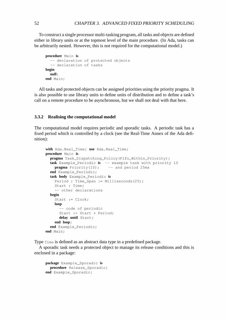
52 CHAPTER 3. ADVANCED FIXED PRIORITY SCHEDULING
To construct a single processor multi-tasking program, all tasks and objects are definedeither in library units or at the topmost level of the main procedure. (In Ada, tasks canbe arbitrarily nested. However, this is not required for the computational model.)
procedure Main is-- declaration of protected objects-- declaration of tasks
beginnull;
end Main;
All tasks and protected objects can be assigned priorities using the priority pragma. Itis also possible to use library units to define units of distribution and to define a task’scall on a remote procedure to be asynchronous, but we shall not deal with that here.
3.3.2 Realising the computational model
The computational model requires periodic and sporadic tasks. A periodic task has afixed period which is controlled by a clock (see the Real-Time Annex of the Ada defi-nition):
with Ada.Real_Time; use Ada.Real_Time;procedure Main is
pragma Task_Dispatching_Policy(Fifo_Within_Priority);task Example_Periodic is -- example task with priority 10
pragma Priority(10); -- and period 25msend Example_Periodic;task body Example_Periodic isPeriod : Time_Span := Milliseconds(25);Start : Time;-- other declarations
beginStart := Clock;loop-- code of periodicStart := Start + Period;delay until Start;
end loop;end Example_Periodic;
end Main;
Type Time is defined as an abstract data type in a predefined package.A sporadic task needs a protected object to manage its release conditions and this is
enclosed in a package:
package Example_Sporadic isprocedure Release_Sporadic;
end Example_Sporadic;

3.4. THE MINE PUMP 53
package body Example_Sporadic istask Sporadic_Thread is
pragma Priority(15);end Sporadic_Thread;protected Starter is
procedure Go;entry Wait;pragma Priority(15); -- ceiling priority
privateRelease_Condition : Boolean := False;
end Starter;procedure Release_Sporadic isbeginStarter.Go;
end Release_Sporadic;task body Sporadic_Thread is
-- declarationsbegin
loopStarter.Wait;-- code of sporadic
end loop;end Sporadic_Thread;protected body Starter is
procedure Go isbeginRelease_Condition := True;
end Go;entry Wait when Release_Condition isbeginRelease_Condition := False;
end Wait;end Starter;
end Example_Sporadic;
The Wait entry must reset the release condition so that its next caller will be blockeduntil Release Sporadic is called again. Variations of this basic structure can deal withbursty releases (with the protected object buffering the releases) and data communicationthrough the protected object from the task that calls Release Sporadic to the sporadictask.
If the sporadic task is to be released by an interrupt then the Go procedure is mappeddirectly onto the interrupt source. An example of this is given in the mine pump examplein the next section.
3.4 The mine pump
Chapter 1 introduced the mine pump control problem. In this section we develop a designusing the computational model defined earlier. A simple decomposition of the systemidentifies four major components:

54 CHAPTER 3. ADVANCED FIXED PRIORITY SCHEDULING
� the pump controller,� the environmental monitors (for airflow, methane and carbon monoxide),� the data logging subsystem,� the operator’s subsystem.
The details of the data logging subsystem will be ignored and a protected object will beused as the interface. Calls to the operator will similarly be mapped onto a protectedobject. The operator can enquire about the status of the pump and attempt to turn thepump on – these operations will be accommodated within the pump controller.
The timing requirements of the environmental monitors have a cyclic behaviour and sothese are represented as periodic tasks. The pump itself is a protected resource and is en-capsulated within a PSO. Whenever the methane monitor reads a critically high methanelevel it will call this PSO to turn the pump off.
The high and low water sensors come into the system as interrupts. It is therefore ap-propriate to define sporadic tasks as the objects that respond to these interrupts and at-tempt to either turn on or turn off the pump (via calls to the pump PSO).
Although this structure provides an adequate design, one piece of functionality is stillmissing: after the methane level returns to low how is the pump turned on again? Thereis also an issue of safety analysis that would normally be applied to this sort of system.With the current design, the methane monitor and the pump controller are safety-critical.It could be argued that the fail-silent behaviour of the monitoring subsystem should notlead to failure (i.e. pump working while methane level too high). This leads to two extraelements being added.
� a PSO Methane Status that holds the current methane level and the time at whichthe data was read (these values are obtained from the methane monitor),
� a periodic task that reads the Methane Status PSO and sends control commandsto the pump controller.
With this structure the new periodic task has the responsibility for turning the pump onagain once the methane level is low enough.
Failure of the methane monitor will lead to a fail-safe state. Of course, this is not a fullyreliable situation as the pump would not be able to operate if the mine were flooding andthe methane level were low.
Figure 3.11 gives a pictorial representation of the design. Table 3.1 gives the details ofthe tasks and PSOs (including a key to the labels used in Figure 3.11). Note that both spo-radic tasks are released by the same PSO. The design could be implemented on a singleprocessor or a distributed system. Figure 3.12 gives one possible distributed configura-tion. Note how all the remote actions are legal in the computational model. One advan-tage of the design of this configuration is that the system fails-silent even when remotecommunications are unreliable.
Table 3.1 shows, where appropriate, the periods and minimum arrival rates of the tasks.It also includes the deadlines and priorities of the tasks (and hence the PSOs). A singleprocessor implementation is assumed and priorities are in the range 1 : : :10; unlike theanalysis in Chapter 2, 1 is the lowest and 10 the highest priority which is allocated to the
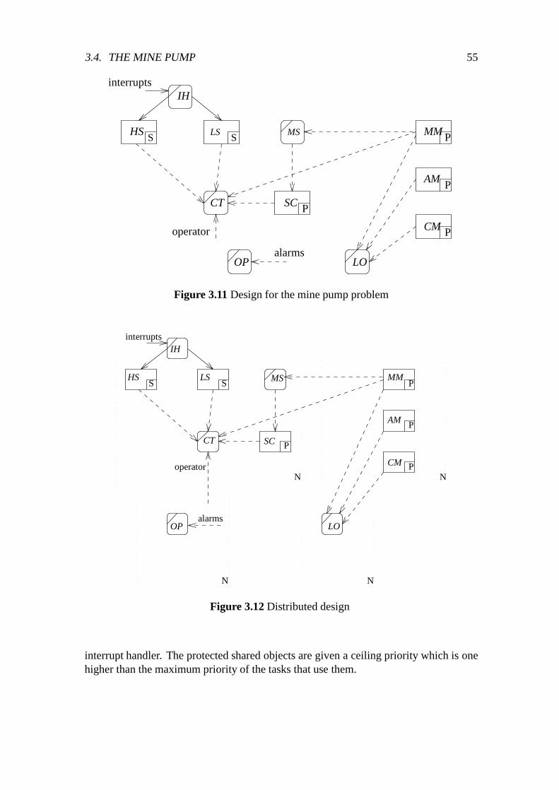
3.4. THE MINE PUMP 55
LS MS
interruptsIH
HSS S
CT
OP
SC P
MM
AM
CM
LO
P
P
Poperator
alarms
Figure 3.11 Design for the mine pump problem
S
alarms
S
interrupts
P
P
P
Poperator
MS
CT
N
NN
N
AM
CM
SC
LSHS
OP LO
MM
IH
Figure 3.12 Distributed design
interrupt handler. The protected shared objects are given a ceiling priority which is onehigher than the maximum priority of the tasks that use them.
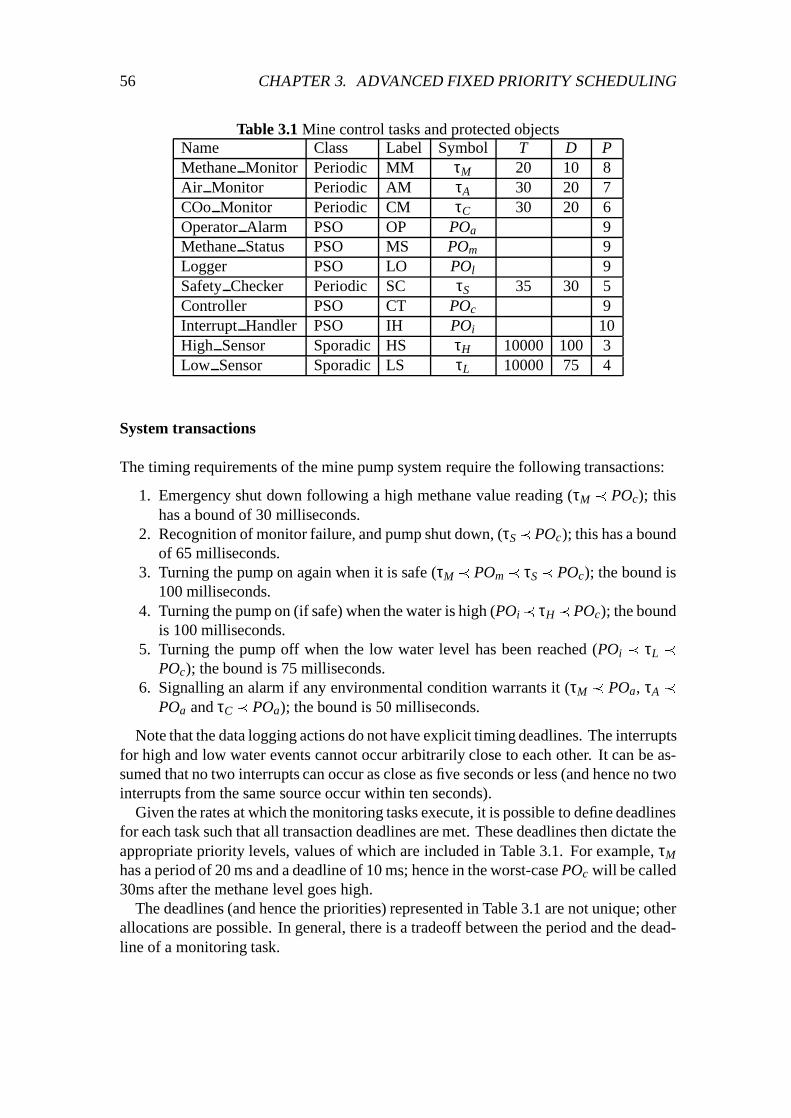
56 CHAPTER 3. ADVANCED FIXED PRIORITY SCHEDULING
Table 3.1 Mine control tasks and protected objectsName Class Label Symbol T D PMethane Monitor Periodic MM τM 20 10 8Air Monitor Periodic AM τA 30 20 7COo Monitor Periodic CM τC 30 20 6Operator Alarm PSO OP POa 9Methane Status PSO MS POm 9Logger PSO LO POl 9Safety Checker Periodic SC τS 35 30 5Controller PSO CT POc 9Interrupt Handler PSO IH POi 10High Sensor Sporadic HS τH 10000 100 3Low Sensor Sporadic LS τL 10000 75 4
System transactions
The timing requirements of the mine pump system require the following transactions:
1. Emergency shut down following a high methane value reading (τM � POc); thishas a bound of 30 milliseconds.
2. Recognition of monitor failure, and pump shut down, (τS�POc); this has a boundof 65 milliseconds.
3. Turning the pump on again when it is safe (τM � POm � τS � POc); the bound is100 milliseconds.
4. Turning the pump on (if safe) when the water is high (POi� τH �POc); the boundis 100 milliseconds.
5. Turning the pump off when the low water level has been reached (POi � τL �POc); the bound is 75 milliseconds.
6. Signalling an alarm if any environmental condition warrants it (τM � POa, τA �POa and τC � POa); the bound is 50 milliseconds.
Note that the data logging actions do not have explicit timing deadlines. The interruptsfor high and low water events cannot occur arbitrarily close to each other. It can be as-sumed that no two interrupts can occur as close as five seconds or less (and hence no twointerrupts from the same source occur within ten seconds).
Given the rates at which the monitoring tasks execute, it is possible to define deadlinesfor each task such that all transaction deadlines are met. These deadlines then dictate theappropriate priority levels, values of which are included in Table 3.1. For example, τM
has a period of 20 ms and a deadline of 10 ms; hence in the worst-case POc will be called30ms after the methane level goes high.
The deadlines (and hence the priorities) represented in Table 3.1 are not unique; otherallocations are possible. In general, there is a tradeoff between the period and the dead-line of a monitoring task.

3.4. THE MINE PUMP 57
3.4.1 Ada 95 implementation
The design objects introduced in the previous section can be coded in Ada 95. The fol-lowing program is for a single processor solution. All the necessary code is included,apart from the instructions that interact with the hardware; these instructions are repre-sented as comments as their actual form would depend upon the particular hardware be-ing used.
Some basic types are first defined in a global package together with constants repre-senting critical input values. For example, if the methane level from the sensor is above32, then the pump should be disabled. The time-constant Freshness indicates the max-imum time a data item should reside within POm without being overwritten by a morerecent reading. Its value is set to T +D for τm.
with Ada.Real_Time; use Ada.Real_Time;package Data_Defs is
type Status is (On,Off);type Safety_Status is (Stopped, Operational);type Alarm_Source is (Methane, Air_Flow, Carbon_Monoxide);type Methane_Value is range 0..256;type Air_Value is range 0..256;type Co_Value is range 0..256;Methane_Threshold : constant Methane_Value := 32;Air_Threshold : constant Air_Value := 100;Co_Threshold : constant Co_Value := 124;Freshness : constant Time_Span := Milliseconds(30);
end Data_Defs;
There are two main protected objects in the program: one gives the current methanereading, the other controls the pump. First consider the simple Methane Status object:
protected Methane_Status isprocedure Read(Ms : out Methane_Value; T : out Time);procedure Write(V : Methane_Value; T : Time);pragma Priority(9);
privateCurrent_Value : Methane_Value := Methane_Value’Last;Time_Of_Read : Time := Clock;
end Methane_Status;protected body Methane_Status is
procedure Read(Ms : out Methane_Value; T : out Time) isbeginMs := Current_Value;T := Time_Of_Read;
end Read;procedure Write(V : Methane_Value; T : Time) isbeginCurrent_Value := V;Time_Of_Read := T;
end Write;end Methane_Status;

58 CHAPTER 3. ADVANCED FIXED PRIORITY SCHEDULING
The pump controller is also a protected object. The sporadic tasks that respond to thehigh and low water interrupts will call Turn On and Turn Off. The safety controller willcall Stop and Start. Only if the status of the pump is on (following a call of Turn On)and the safety status is operational (i.e. no call of Stop) will the pump be actually started(or restarted). The other subprogram defined in this object is called by the operator mod-ule:
protected Controller isprocedure Turn_On;procedure Turn_Off;procedure Stop;procedure Start;procedure Current_Status(St:out Status;
Safe_St:out Safety_Status);pragma Priority(9);
privatePump : Status := Off;Condition : Safety_Status := Stopped;
end Controller;protected body Controller is
procedure Turn_On isbeginPump := On;if Condition = Operational then-- turn on pump
end if;end Turn_On;procedure Turn_Off isbeginPump := Off;-- turn off pump
end Turn_Off;procedure Stop isbegin-- turn off pumpCondition := Stopped;
end Stop;procedure Start isbeginCondition := Operational;if Pump = On then-- turn on pump
end if;end Start;procedure Current_Status(St:out Status;
Safe_St:out Safety_Status) isbeginSt := Pump;Safe_St := Condition;
end Current_Status;end Controller;
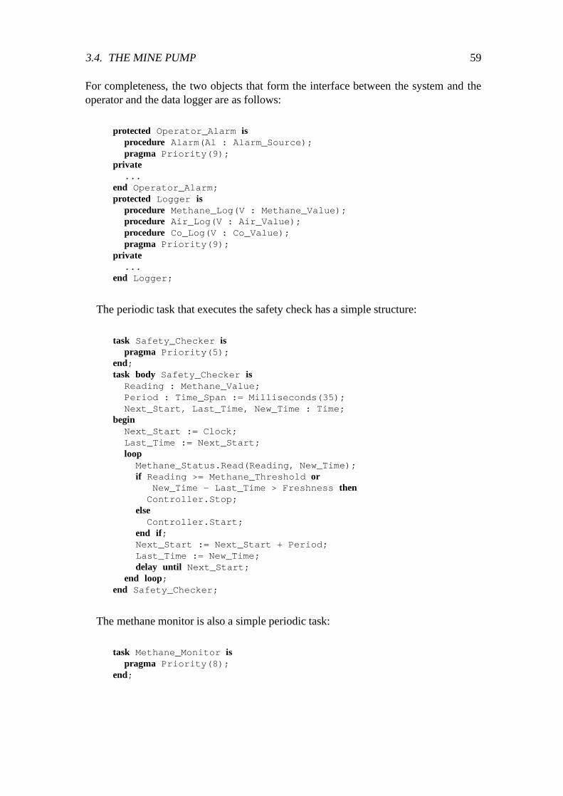
3.4. THE MINE PUMP 59
For completeness, the two objects that form the interface between the system and theoperator and the data logger are as follows:
protected Operator_Alarm isprocedure Alarm(Al : Alarm_Source);pragma Priority(9);
private...
end Operator_Alarm;protected Logger is
procedure Methane_Log(V : Methane_Value);procedure Air_Log(V : Air_Value);procedure Co_Log(V : Co_Value);pragma Priority(9);
private...
end Logger;
The periodic task that executes the safety check has a simple structure:
task Safety_Checker ispragma Priority(5);
end;task body Safety_Checker is
Reading : Methane_Value;Period : Time_Span := Milliseconds(35);Next_Start, Last_Time, New_Time : Time;
beginNext_Start := Clock;Last_Time := Next_Start;loopMethane_Status.Read(Reading, New_Time);if Reading >= Methane_Threshold or
New_Time - Last_Time > Freshness thenController.Stop;
elseController.Start;
end if;Next_Start := Next_Start + Period;Last_Time := New_Time;delay until Next_Start;
end loop;end Safety_Checker;
The methane monitor is also a simple periodic task:
task Methane_Monitor ispragma Priority(8);
end;

60 CHAPTER 3. ADVANCED FIXED PRIORITY SCHEDULING
task body Methane_Monitor isSensor_Reading : Methane_Value;Period : Time_Span := Milliseconds(20);Next_Start : Time;
beginNext_Start := Clock;loop-- read hardware register into Sensor_Reading;if Sensor_Reading >= Methane_Threshold thenController.Stop;Operator_Alarm.Alarm(Methane);
end if;Methane_Status.Write(Sensor_Reading,Next_Start);Logger.Methane_Log(Sensor_Reading);Next_Start := Next_Start + Period;delay until Next_Start;
end loop;end Methane_Monitor;
To complete the software for the periodic structures, the tasks for air monitoring andcarbon monoxide monitoring are as follows:
task Air_Monitor ispragma Priority(7);
end;task body Air_Monitor is
Sensor_Reading : Air_Value;Period : Time_Span := Milliseconds(30);Next_Start : Time;
beginNext_Start := Clock;loop-- read hardware register into Sensor_Reading;if Sensor_Reading <= Air_Threshold thenOperator_Alarm.Alarm(Air_Flow);
end if;Logger.Air_Log(Sensor_Reading);Next_Start := Next_Start + Period;delay until Next_Start;
end loop;end Air_Monitor;task Co_Monitor is
pragma Priority(6);end Co_Monitor;task body Co_Monitor is
Sensor_Reading : Co_Value;Period : Time_Span := Milliseconds(30);Next_Start : Time;

3.4. THE MINE PUMP 61
beginNext_Start := Clock;loop-- read hardware register into Sensor_Reading;if Sensor_Reading >= Co_Threshold thenOperator_Alarm.Alarm(Carbon_Monoxide);
end if;Logger.Co_Log(Sensor_Reading);Next_Start := Next_Start + Period;delay until Next_Start;
end loop;end Co_Monitor;
The two sporadic tasks are closely related and can therefore be managed by the sameprotected object:
package Flow_Sensors istask High_Sensor is
pragma Priority(4);end High_Sensor;task Low_Sensor is
pragma Priority(3);end Low_Sensor;
end Flow_Sensors;package body Flow_Sensors is
protected Interrupt_Handlers isprocedure High; pragma Interrupt_Handler(High);procedure Low; pragma Interrupt_Handler(Low);entry Release_High; entry Release_Low;pragma Priority(10);
privateHigh_Interrupt, Low_Interrupt : Boolean := False;
end Interrupt_Handlers;protected body Interrupt_Handlers is
procedure High isbeginHigh_Interrupt := True;
end High;procedure Low isbeginLow_Interrupt := True;
end Low;entry Release_High when High_Interrupt isbeginHigh_Interrupt := False;
end Release_High;entry Release_Low when Low_Interrupt isbeginLow_Interrupt := False;
end Release_Low;end Interrupt_Handlers;

62 CHAPTER 3. ADVANCED FIXED PRIORITY SCHEDULING
Table 3.2 Worst case execution timesName Class Symbol CMethane Monitor Periodic τM 5:4Air Monitor Periodic τA 3:3CO Monitor Periodic τC 3:3Safety Checker Periodic τS 3:5Low Sensor Sporadic τL 2:9High Sensor Sporadic τH 2:9Interrupt Handler PSO POi 1:2Controller PSO POc 1:4Operator Alarm PSO POa 0:1Methane Status PSO POm 1.2Logger PSO POl 0:8
task body High_Sensor isbegin
loopInterrupt_Handlers.Release_High; Controller.Turn_On;
end loop;end High_Sensor;task body Low_Sensor isbegin
loopInterrupt_Handlers.Release_Low; Controller.Turn_Off;
end loop;end Low_Sensor;
end Flow_Sensors;
This completes the code for all of the components of the design.
3.4.2 Analysis of the application
Once the code has been developed it must be analyzed to obtain its worst-case executiontimes. As indicated in Section 3.2.1, these values can be obtained either by direct mea-surement or by modelling the hardware. None of the code derived is likely to requireextensive computations and so it is reasonable to assume that a slow speed processoris adequate. Table 3.2 contains some representative values for the worst-case executiontimes for each task and PSO in the design. Note that the times for each task include timespent executing within called PSOs. Hence, for example, τM will call POm and POl ineach period but will also call POc and POa when the methane is high. This gives a totalof 5.4 milliseconds of execution time.
The execution environment imposes its own set of important parameters – these are
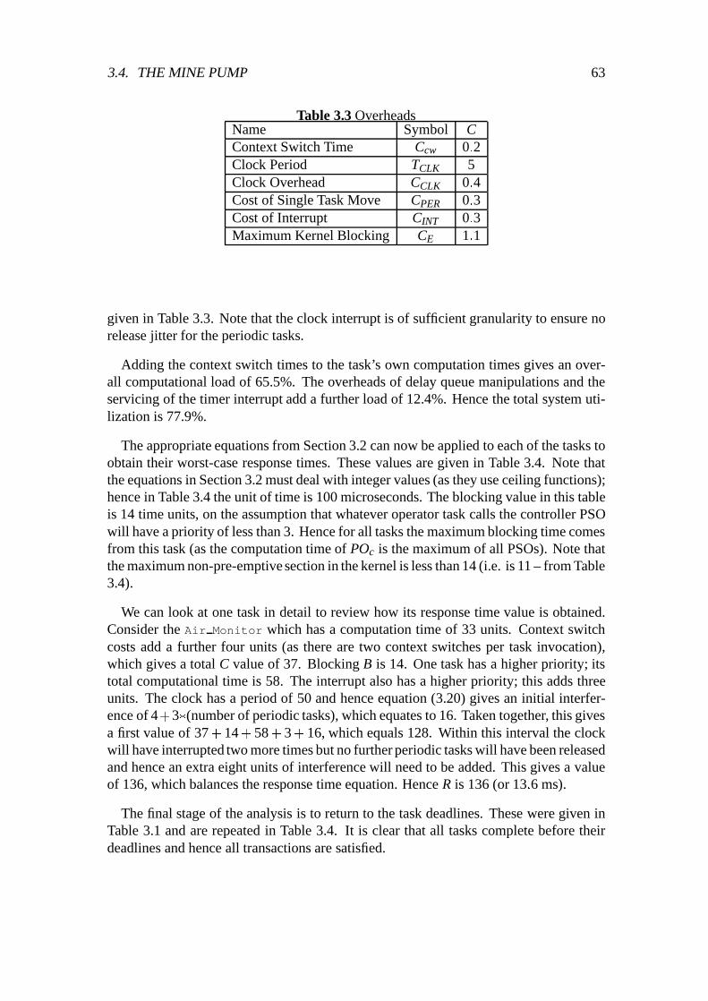
3.4. THE MINE PUMP 63
Table 3.3 OverheadsName Symbol CContext Switch Time Ccw 0:2Clock Period TCLK 5Clock Overhead CCLK 0:4Cost of Single Task Move CPER 0:3Cost of Interrupt CINT 0:3Maximum Kernel Blocking CE 1:1
given in Table 3.3. Note that the clock interrupt is of sufficient granularity to ensure norelease jitter for the periodic tasks.
Adding the context switch times to the task’s own computation times gives an over-all computational load of 65.5%. The overheads of delay queue manipulations and theservicing of the timer interrupt add a further load of 12.4%. Hence the total system uti-lization is 77.9%.
The appropriate equations from Section 3.2 can now be applied to each of the tasks toobtain their worst-case response times. These values are given in Table 3.4. Note thatthe equations in Section 3.2 must deal with integer values (as they use ceiling functions);hence in Table 3.4 the unit of time is 100 microseconds. The blocking value in this tableis 14 time units, on the assumption that whatever operator task calls the controller PSOwill have a priority of less than 3. Hence for all tasks the maximum blocking time comesfrom this task (as the computation time of POc is the maximum of all PSOs). Note thatthe maximum non-pre-emptive section in the kernel is less than 14 (i.e. is 11 – from Table3.4).
We can look at one task in detail to review how its response time value is obtained.Consider the Air Monitor which has a computation time of 33 units. Context switchcosts add a further four units (as there are two context switches per task invocation),which gives a total C value of 37. Blocking B is 14. One task has a higher priority; itstotal computational time is 58. The interrupt also has a higher priority; this adds threeunits. The clock has a period of 50 and hence equation (3.20) gives an initial interfer-ence of 4+3�(number of periodic tasks), which equates to 16. Taken together, this givesa first value of 37+ 14+ 58+ 3+ 16, which equals 128. Within this interval the clockwill have interrupted two more times but no further periodic tasks will have been releasedand hence an extra eight units of interference will need to be added. This gives a valueof 136, which balances the response time equation. Hence R is 136 (or 13:6 ms).
The final stage of the analysis is to return to the task deadlines. These were given inTable 3.1 and are repeated in Table 3.4. It is clear that all tasks complete before theirdeadlines and hence all transactions are satisfied.

64 CHAPTER 3. ADVANCED FIXED PRIORITY SCHEDULING
Table 3.4 Results of schedulability analysisName Class Symbol T D P C RMethane Monitor Periodic τM 200 100 8 58 95Air Monitor Periodic τA 300 200 7 37 136CO Monitor Periodic τC 300 200 6 37 177Safety Checker Periodic τS 350 300 5 39 285Low Sensor Sporadic τL 100000 750 4 33 525High Sensor Sporadic τH 100000 1000 3 33 558
3.5 Historical background
The computational model presented in this chapter is similar to that used in a number ofdesign methods such as Mascot (Bate, 1986) and HRT-HOOD (Burns & Wellings, 1994).A formal representation of the model can be found in the semantic descriptions of theTemporal Access Method (TAM) (Scholfield et al., 1994).
Section 3.2 gave an overview of some recent scheduling results; the derivation of theseequations is described in Burns (1994), Audsley et al. (1993a; 1993b) and Burns etal. (1993), and detailed descriptions have been provided by Audsley (1993) and Tindell(1993). Discussion of the inheritance and ceiling protocols can be found in Goodenoughand Sha (1988), Sha et al. (1990) and Baker (1990; 1991). A detailed case study of theAltitude and Orbital Control System (AOCS) of the Olympus Satellite appears in Burnset al. (1993).
Debates over the development of the Ada programming language have raged for anumber of years. Readers interested in issues relating to the Ada tasking model will finda discussion in Burns et al. (1987). Real-time issues are discussed extensively in theProceedings of the International Workshops on Real-Time Ada Issues.3
3.6 Further work
The analysis presented in this chapter covers a level of detail and a range of practical con-cerns that make it suitable for use on ‘real’ systems. There is current research in increas-ing the flexibility of the analysis and further removing restrictions in the computationalmodel. For example, the model can be extended to include invocation interruption (i.e.asynchronously affecting the execution of a periodic task, during execution, to allow itto respond immediately to a mode change), dynamic allocation and re-allocation to caterfor processor failure.
There has been much attention recently to the use of on-line techniques because, it isargued, that contemporary systems are too complex for purely off-line analysis. On-line
3The proceedings of these workshops, which started in 1987, are published annually in ACM AdaLetters.

3.7. EXERCISES 65
techniques are based on ‘best-effort’ scheduling to make the most effective use of thesystem under all possible conditions; they will be described in greater detail in Chapter4. While priority-based scheduling and best-effort scheduling are often considered to beirreconcilable, there has been work on defining a framework that can accommodate bothapproaches (Audsley et al., 1993c; 1994; Davis et al., 1993). Within such a frameworkit would be possible to integrate static analysis, diverse and adaptive software, deadlinevariations and software fault-tolerance (Bondavalli et al., 1993).
3.7 Exercises
Exercise 3.1 Verify that the system transaction deadlines for the mine control problemare satisfied by the period and deadline definitions in given Table 3.1.
Exercise 3.2 Check the response-time calculations given in Table 3.4. Which value iswrong?
Exercise 3.3 In the analysis of the mine control system, what would be the conse-quences of running the clock at 10 ms (or 20 ms)?
Exercise 3.4 Do a sensitivity analysis on the mine control task set. Taking each taskin turn, consider by how much its computation time must increase before the task setbecomes unschedulable. Express this value as a percentage of the original value of thecomputation time.

Chapter 4
Dynamic Priority Scheduling
Krithi Ramamritham
Introduction
Dynamic scheduling of a real-time program requires a sequence of decisions to be takenduring execution on the assignment of system resources to transactions. Each decisionmust be taken without prior knowledge of the needs of future tasks. As in the case offixed priority scheduling, the system resources include processors, memory and shareddata structures; but tasks can now have arbitrary attributes: arrival times, resource re-quirements, computation times, deadlines and importance values.
Dynamic algorithms are needed for applications where the computing requirementsmay vary widely, making fixed priority scheduling difficult or inefficient. Many real-timeapplications require support for dynamic scheduling: e.g. in robotics, where the controlsubsystem must adapt to a dynamic environment. This kind of scheduling also allowsmore flexibility in dealing with practical issues, such as the need to alter scheduling de-cisions based on the occurrence of overloads, e.g. when
� the environment changes,� there is a burst of task arrivals, or� a part of the system fails.
In a practical system, it can prove costly to assume that overloads and failures will neveroccur and, at the same time, be inefficient to determine schedulability or a priori to con-struct a fixed schedule for a system with such variable properties.
Dynamic scheduling has three basic steps: feasibility checking, schedule constructionand dispatching. Depending on the kind of application for which the system is designed,the programming model adopted and the scheduling algorithm used, all of the steps maynot be needed. Often, the boundaries between the steps may also not be clear.
We shall first generalize the definitions of transaction and process used in Chapter 3. Acomputational transaction will now be assumed to be made up of one or more processescomposed in parallel. A process consists of one or more tasks.
66

INTRODUCTION 67
Feasibility analysisFeasibility, or schedulability, analysis has been described in Chapters 2 and 3: it is theprocess of determining whether the timing requirements of a set of tasks can be satis-fied, usually under a given set of resource requirements and precedence constraints. Withfixed priority scheduling, feasibility analysis is typically done statically, before the pro-gram is executed. Dynamic systems perform feasibility checking on-line, as tasks arrive.
There are two approaches to scheduling in dynamic real-time systems:
1. Dynamic planning-based approaches: Execution of a task is begun only if it passesa feasibility test, i.e that it will complete execution before its deadline. Often, oneof the results of the feasibility analysis is a schedule or plan that is used to decidewhen a task should begin execution.
2. Dynamic best-effort approaches: Here no feasibility checking is done; the systemtries to ‘do its best’ to meet deadlines but, since feasibility is not checked, a taskmay be aborted during its execution.
In a planning-based approach, the feasibility of a set of tasks is checked in terms of ascheduling policy such as ‘earliest-deadline-first’ or ‘least-laxity-first’, before the execu-tion of a set of tasks. By contrast, in a best-effort approach, tasks may be queued accord-ing to policies that take account of the time constraints (similar to the kind of schedulingfound in a non-real-time operating system). No feasibility checking is done before thetasks are queued.
The relative importance of a task and the value given to its completion are used totake scheduling decisions, whether or not feasibility checking is done. This informationis usually given as a time-value function that specifies the contribution of a task to thesystem upon its successful completion. Figure 4.1 relates value with completion time,for different value functions.
For hard real-time tasks, the value drops immediately after the deadline and dynamicalgorithms cannot be used: there should be a priori verification that such tasks will meettheir deadlines. Dynamic algorithms are suitable for the tasks in the ‘firm’ and ‘soft’categories.
To achieve high system performance, the system must also consider the relative valuesof tasks, or their importance, when determining which tasks to reject and which to exe-cute. Because a dynamic scheduling algorithm takes decisions without prior knowledgeof the tasks, the total value is not predictable and the algorithm must attempt to maximizethe value accrued from tasks that complete on time. Most dynamic algorithms developedso far assume that a value function assigns a positive value to a task that is successfullycompleted, and zero to an incomplete task. This corresponds to the curve marked ‘firm’in Figure 4.1, where the value for a task remains constant until its deadline and then dropsto zero. If all the tasks have the same value, maximizing the accrued value is the sameas maximizing the number of completed tasks.
While achieving maximum value, real-time systems must also exhibit a capability for‘graceful degradation’. To achieve this, not only must the fact that a task did not meet itsdeadline be detected, but the fact that this is going to occur must be detected as soon as

68 CHAPTER 4. DYNAMIC PRIORITY SCHEDULING
time
hard
firm
soft
value
Figure 4.1 Different kinds of value function
possible. An exception must then be signalled to make it possible for the task to be substi-tuted by one or more contingency tasks. Thus on-line schedulability analysis must havean early warning feature which provides sufficient lead time for the timely invocation ofcontingency tasks, making it possible for the scheduler to take account of a continuouslychanging environment.
Such schedulability analysis is especially important for transactions for which recov-ery following an aborted partial execution can be complicated. Error handlers are com-plex in general and abnormal termination may produce inconsistent system states. Thisis likely to be the case especially if the transaction involves inter-process interaction. Insuch situations, it is better to allow a transaction to take place only if it can be guaranteedto complete by its deadline. If such a guarantee cannot be provided, then the program canperform an alternative action. And to provide sufficient time for executing the alterna-tive action, a deadline may be imposed on the determination of schedulability. This canbe generalized so that there are N versions of the transaction and the algorithm attemptsto guarantee the execution of the best possible version. ‘Best’ refers to the value of theresults produced by a particular version; typically, the better the value of the result, thelonger the execution time.
Schedule constructionSchedule construction is the process of ordering the tasks to be executed and storing thisin a form that can be used by the dispatching step.
Feasibility checking is sometimes performed by checking if there is a schedule or planin which all the tasks will meet their deadlines. For planning-based approaches, scheduleconstruction is usually a direct consequence of feasibility checking.
In other cases, priorities are assigned to tasks and at run-time the task in execution

4.1. PROGRAMMING DYNAMIC REAL-TIME SYSTEMS 69
has the highest priority. This is the case with fixed priority approaches and with somesimple dynamic priority approaches, such as earliest-deadline-first or least-laxity-first,where feasibility checking involves ensuring that the total processor utilization is belowa bound.
In the remainder of this chapter we will refer to schedule construction simply asscheduling. Thus, scheduling involves deciding when tasks will execute. The scheduleis maintained explicitly in the form of a plan or implicitly as the assignment of prioritiesto tasks.
DispatchingDispatching is the process of deciding which task to execute next. The complexity andrequirements for the dispatching step depend on:
1. the scheduling algorithm used in the feasibility checking step,2. whether a schedule is constructed as part of the schedulability analysis step,3. the kinds of tasks, e.g. whether they are independent or with precedence con-
straints, and whether their execution is pre-emptive or non-pre-emptive, and4. the nature of the execution platform, e.g. whether it has one processor or more and
how communication takes place.
For example, with non-pre-emptive scheduling a task is dispatched exactly once; withpre-emptive scheduling, a task will be dispatched once when it first begins execution andagain whenever it is resumed.
In the remainder of this chapter, we discuss how the timing requirements of transac-tions can be specified and how user level transactions can be mapped into tasks withdifferent characteristics including timing constraints, precedence constraints, resourcerequirements, importance levels and communication characteristics. Issues to be con-sidered for dynamic scheduling are introduced and different ways of assigning priori-ties to tasks are considered. The two types of dynamic scheduling approach, best-effortscheduling and planning-based scheduling, are discussed in detail and, since the run-timecost of a dynamic approach is an important practical consideration, several techniques arediscussed for efficient dynamic scheduling.
4.1 Programming dynamic real-time systems
The requirements for tasks in a real-time system can be quite varied. In this section, weshow how they can be specified from within a program. For dynamic real-time applica-tions, it should be possible to specify several important requirements:
� Before initiating a time-constrained transaction, it should be possible for the pro-gram to ask for a guarantee from the run-time system that the transaction will becompleted within the specified deadline.
70 CHAPTER 4. DYNAMIC PRIORITY SCHEDULING
A transaction can be guaranteed to complete within its deadline if a schedule canbe created for this transaction and the other transactions that have been previouslyguaranteed to meet their deadlines.
� If the system cannot give a guarantee when it is sought, then it should be possibleto choose an alternative activity. When a guarantee is not sought and it is not pos-sible to meet the timing constraint, it should be possible to take alternative action.In either case, the alternative may be a timing-error handler that will allow somecorrective action to be taken.
Language constructs to express such constraints are described using a form of pseudo-code. In what follows, terminals are shown in typewriter font, [ ] encloses optionalitems and | separates alternatives.
A transaction (shown in italics) refers to a statement. A real-time transaction has atime constraint such as a periodicity requirement or a deadline.
4.1.1 Activities with deadlines
Timeouts can be associated with any statement using the within deadline statementwhich has the form
within deadline (d) statement1[ else statement2 ]
During execution, if execution of a within deadline statement starts at time t and is notcompleted by t+d, then it is terminated and statement2, if provided, is executed. Hence,d is the deadline relative to the current time. The effect of this abnormal terminationis local if statement1 does not require any inter-process communication; otherwise, theother interacting processes may be affected. We discuss this further in Section 4.1.5.
Example 4.1 Air traffic control 1. An air-traffic control system should provide finalclearance for a pilot to land within 60 seconds after clearance is requested. Otherwisethe pilot will abort the landing procedure:
within deadline (60) get clearanceelse abort landing
4.1.2 Guaranteed transactions
The guarantee statement is used to ensure before a transaction is started that it can becompleted within the specified time constraint:
within deadline (gd ) guarantee
time constrained statement[else statement ]

4.1. PROGRAMMING DYNAMIC REAL-TIME SYSTEMS 71
where gd is the deadline for obtaining the guarantee. If the guarantee is not possible, orif it cannot be given within gd, the else statement, if provided, is executed. Otherwise,the time-constrained statement is executed.
To provide such a guarantee, the execution time and the resource requirements of thestatement must a priori be determinable (at least at the time of the guarantee). This makesit important for the execution time to lie within relatively small bounds as resources mustbe provided for the worst-case needs. In general, the larger the worst-case needs, the lesslikely it will be to obtain a guarantee; further, even if a guarantee can be given for largebounds, it is likely to affect future guarantees.
Dynamic scheduling makes it possible to use run-time information about tasks, such asexecution times and resource constraints. Such information can be derived from formu-las provided by the compiler for evaluation at the time of task invocation. For example,the calculation of the execution time can then take into account the specific parametersof the invocation and hence be more accurate (and perhaps less pessimistic) than a stat-ically determined execution time; such calculations can make use of data only availableat run-time, such as the number and values of inputs. As for compile-time calculation ofworst-case execution times, run-time calculation also requires loop iterations and com-munication times to be bounded. If synchronous communication statements do not haveassociated time-constraints, it is necessary to consider the communicating tasks togetheras a transaction when checking feasibility.
Example 4.2 The following statement tries to guarantee that statement1 will be com-pleted within the next d seconds:
within deadline (gd) guarantee
within deadline (d) statement1[else ...]
[else statement2 ]
If execution starts at time t, statement2 will be executed if it is not possible to obtain theguarantee by t + gd. If guaranteed, execution of statement1 will start at st and end by t+ d, where st lies in the interval (t; t+gd).
Example 4.3 A simple railway crossing. The task controlling a railway signal has todetermine whether a certain track will be clear by the time a train is expected to reachthere. This must be done early enough to give enough time to stop the train if the track isnot expected to be clear. Assume that the train will not reach the track before d secondsand that it takes at most s seconds to stop the train (s < d):
within deadline (d� s) guarantee
within deadline (d) clear trackelse ...
else stop train

72 CHAPTER 4. DYNAMIC PRIORITY SCHEDULING
4.1.3 Start-time-constraints
The following statement attaches start time constraints to transactions with deadlines:
start at (s) within deadline (d ) statement1[else statement2]
If execution of the within deadline statement starts at time t, then execution ofstatement1 should start at or after t+ s and be completed by t+d, where d > s. A simpleextension gives the guaranteed version of this statement.
The value v of a task is specified by attaching the construct value v to the within
deadline statement.
4.1.4 Flexible time-constraints
The time-constraints described thus far are to ensure that if a transaction is not completedwithin the specified time, it is terminated and timing-error handling is done. This is ap-propriate if there is no value in completing the transaction after the specified time.
For many real-time applications, while it may be desirable for all transactions to meetthe timing-constraints, it may be better, and sometimes necessary, to complete a transac-tion even if it is delayed. Such time-constraints will be called flexible. Thus a transactionmay have a non-zero value up to some point past its deadline; if this point does not lie ina fixed interval, the transaction should be completed regardless of how long it takes.
To express flexible time-constraints, an overflow is associated with a time-constraint.If the overflow is positive, a transaction should be terminated only after the end of theinterval corresponding to the overflow. This corresponds to a soft deadline.
If the overflow has a negative value, it indicates that the transaction must be completedby the specified deadline but, if possible, within overflow units before the deadline. (Thisis like asking the system to ‘be nice’ to a transaction by trying to complete it before thedeadline.)
A deadline-constrained transaction statement1 is specified as
within deadline (d)[overflow] statement1else statement2
and has the following effect:
� If execution of statement1 is not completed by max(d;d+overflow), processing ofstatement1 is terminated and statement2, if provided, is executed.
� If overflow is not specified, it is assumed to be zero.� If a guarantee is requested, it will be first attempted for min(d;d+overflow) and,
if this is unsuccessful, for max(d;d+ overflow); if the second attempt is also un-successful, the else clause, if specified, will be executed.
� If a time-constrained component of statement1 has an overflow, it can increase theworst-case execution time of statement1.

4.1. PROGRAMMING DYNAMIC REAL-TIME SYSTEMS 73
Example 4.4 Air traffic control 2. An air-traffic control system should provide finalclearance for a pilot to land within t1 seconds after the request has been made; if this isnot possible, clearance should be given within another t2 seconds or the pilot will abortthe landing procedure:
within deadline (t1) (t2) clear landingelse abort landing
It is easy to see that a large overflow indicates that the transaction has only a nominaldeadline and should be allowed to complete even if the deadline is past.
4.1.5 Inter-process communication and time-constraints
There are two important considerations when a time-constrained transaction interactswith other transactions. The first is to find the duration of such interactions so that theexecution time of the transaction can be determined. The second is the effect on othertransactions when a time-constrained transaction is terminated because a specified time-constraint is not met.
The sender of an asynchronous message does not wait (assuming that buffers do notoverflow), so the time needed for sending a message is bounded. However, for syn-chronous communication, the sending task is suspended until the receiver responds andthe delay may be unbounded. With timed synchronous communication, the maximumtime that a task can wait for a call to complete is bounded.
The execution of a statement with an associated deadline is abandoned when its dead-line has expired, and there are a number of consequences when a synchronous send orreceive statement is abandoned by the callee:
� A send that is abandoned before the matching receive occurs will clearly not af-fect the sender. If it is withdrawn during the execution of the receive statement,there is no effect on the receiver. It should be possible for the sender to determineif the message was received or if it was withdrawn while in the process of beingreceived. A special variable t interrupted can be associated with each task toindicate if the last send was withdrawn during the receive.
� A similar variable t abandoned can be used to indicate if execution of a receivestatement was abandoned by the receiver.
Example 4.5 Termination during process interaction. A resource is managed by aManager task. If a requesting task has not received the resource within max wait time itwill take its request to another provider:
within deadline (max wait)Manager.get(pid)
else get resource from another provider

74 CHAPTER 4. DYNAMIC PRIORITY SCHEDULING
where pid is the id of the calling task.The Manager task may be responding to the get request when the specified time limit
max wait expires. In this case, although the request is withdrawn, the Manager contin-ues with the allocation as if nothing happened and the requester is required to free theresource after examining the value of variable t interrupted:
within deadline (max wait)Manager.get(pid)
else if (t interrupted) then Manager.free(pid);
get resource from another provider
Let us now examine what is involved in guaranteeing whether or not a synchronoussend can be completed within a deadline:
within deadline (d) guarantee
within deadline (max wait) Manager.get(pid);
else get resource from another provider;
To provide this guarantee, the scheduler must be able to determine when the receiver willactually receive the message. In some special cases, it may be possible to determine thistime but, in general, the delay may depend on a number of factors such as the executiontimes of various code segments within the receiver, when these code segments will bescheduled, etc. Taken together, they make it all but impossible for the sender to determinedynamically when the receiver will receive the message.
However, in the special case of a set of interacting tasks participating in a transactionwith a deadline, the transaction can be converted into a set of precedence-related tasksand started only if they are found to be feasible.
A transaction may be suspended at a number of scheduling points; these occur at thebeginning and end of critical sections, at synchronous communication calls, or whereexplicit suspend calls appear in the code. A transaction is executed from one schedulingpoint to the next (a task) and it can then be executed without being interrupted for wantof resources or for synchronization.
A task graph contains tasks related by precedence and communication constraints. Ac-tivities without internal scheduling points reduce to a graph with a single task. Activitiescontaining critical sections or other scheduling points will reduce to task graphs with sev-eral tasks. During the construction of the task graph, the resources needed for each taskcan be determined. The description of a transaction is then available for the scheduler asa group of tasks representing the transaction.
Figure 4.2 shows a transaction with two components A and B which can execute inparallel and communicate synchronously. This transaction is converted into a graph withfive tasks. With this, the two components, and hence the transaction, can be executedpredictably if the corresponding task graph can be feasibly scheduled.

4.2. ISSUES IN DYNAMIC SCHEDULING 75
B2Synch Synch
A BA1 B1
A2 B3
send rec.
Precedence constraint
Communication
Figure 4.2 Communicating tasks and the corresponding task graph
4.2 Issues in dynamic scheduling
With static priorities, a task’s priority is assigned when it arrives and fresh evaluationis not required as time progresses and new tasks arrive. Hence static priorities are wellsuited for periodic tasks that execute at all times (but, with the extensions shown in Chap-ter 3, they can be used for aperiodic tasks as well).
In a dynamic system, static feasibility checking is not possible and dynamic decisionmaking algorithms must be used. This has several implications. It is no longer possibleto guarantee that all task arrivals will be able to meet their deadlines: if the arrival timesof tasks are not known, the schedulability of the tasks cannot be guaranteed. However, ifthe system has only independent, periodic tasks and one processor, static schedulabilityanalysis can be used even if the scheduling policy is dynamic.
For tasks with a more complex structure, other attributes can be used to assign prior-ities. This gives dynamic algorithms a lot of flexibility and adds to their ability to dealwith a wide variety of tasks. But there may be substantial overheads in calculating thepriorities of tasks and in selecting the task of highest priority. When dynamic prioritiesare used, the relative priorities of tasks can change as time progresses, as new tasks arriveor as tasks execute. Whenever one of these events occurs, the priority of all the remain-ing tasks must be recomputed. This makes the use of dynamic priorities more expensivein terms of run-time overheads, and in practice these overheads must be kept as small aspossible.
A shortcoming of static schedulability analysis arises from the assumptions and therestrictions on which off-line guarantees are based. For example, if there is a non-zeroprobability that these assumptions are unlikely to hold or that restrictions may be vi-olated, a system using a static approach will not perform as designed and tasks maymiss their deadlines. And, under some situations, effective control of the system canbe lost because of the limited scheduling capability available at run-time. Thus, whenconstraints assumed by off-line schedulability analysis are likely to be violated, dynamic

76 CHAPTER 4. DYNAMIC PRIORITY SCHEDULING
scheduling approaches provide a solution.Consider a very simple example. If system overloads are known to be impossible, then
the earliest-deadline-first algorithm (EDF) can be used. Since overloads cannot occur,when a task is pre-empted there is an implicit guarantee that the remainder of the taskwill be completed before its deadline; without overloads, simple algorithms such as EDFand least-laxity-first (LLF) perform very well. But if overloads are possible, in the worstcase, EDF and LLF may produce zero value, i.e. none of the tasks that arrive will meet itsdeadline (even if, under another scheduling discipline, some tasks may meet their dead-lines).
An optimal dynamic scheduling algorithm always produces a feasible schedule when-ever a clairvoyant algorithm, i.e. a scheduling algorithm with complete prior knowledgeof the tasks, can do so. Unfortunately, it is difficult to construct a good on-line algo-rithm to compete with a clairvoyant algorithm. Competitiveness analysis, involving thecomparison of an on-line algorithm with a clairvoyant algorithm, is one way to predictthe behaviour of a dynamic algorithm. However, this analysis considers only worst-casebehaviours involving all possible task characteristics. For predictability, planning-basedscheduling is a viable alternative. Here, given a particular priority assignment policy andthe requirements of a task before it begins execution, a check is made to see whetherthere is a way for the task to meet its deadline. As mentioned earlier, many planning ap-proaches also produce a schedule for task execution as a useful by-product and the addedcost of the checking may be well spent.
4.3 Dynamic priority assignment
Construction of a plan in planning-based approaches and determining which task to ex-ecute next in best-effort approaches requires assigning priorities to tasks; this raises thequestion of how priorities are assigned. Further, there is a conflict between priority-basedscheduling and the goal of maximizing resource utilization in a real-time system.
4.3.1 Simple priority assignment policies
In a real-time system, priority assignment must be related to the time constraints asso-ciated with a task, e.g. according to EDF or LLF ordering. For scheduling independenttasks with deadline constraints on single processors, EDF and LLF are optimal methods,so if any assignment of priorities can feasibly schedule such tasks, then so can EDF andLLF.
For a given task set, if tasks have the same arrival times but different deadlines, EDFgenerates a non-pre-emptive schedule, while the LLF schedule requires pre-emptions. Ifboth arrival times and deadlines are arbitrary, EDF and LLF schedules may both requirepre-emptions. These algorithms use the timing characteristics of tasks and are suitablewhen the processor is the only resource needed and tasks are independent of each other.

4.3. DYNAMIC PRIORITY ASSIGNMENT 77
4.3.2 Priority assignment for tasks with complex requirements
Of more practical interest is the scheduling of tasks with timing constraints, precedenceconstraints, resource constraints and arbitrary values on multi-processors. Unfortunately,most instances of the scheduling problem for real-time systems are computationally in-tractable. Non-pre-emptive scheduling is desirable as it avoids context switching over-heads, but determining such a schedule is an NP-hard problem even on uniprocessors iftasks can have arbitrary ready times. The presence of precedence constraints exacerbatesthe situation and finding a resource-constrained schedule is an NP-complete problem.
This makes it clear that it serves no effective purpose to try to obtain an optimal sched-ule, especially when decisions are made dynamically. And, with multi-processors, no dy-namic scheduling algorithm is optimal and can guarantee all tasks without prior knowl-edge of task deadlines, computation times and arrival times. Such knowledge is not avail-able in dynamic systems so it is necessary to resort to approximate algorithms or to useheuristics, as we shall now see.
As in Chapter 3, a task τ is the unit for scheduling; it is characterized by its arrivaltime AT, its absolute deadline D, its value V, its worst-case computation time C and itsresource requirements fRRg. Tasks are assumed to be independent, non-periodic andnon-pre-emptive. A task uses a resource either in shared mode or in exclusive mode andholds a requested resource as long as it executes. EST is the earliest start time at whichthe task can begin execution (EST is calculated when scheduling decisions are made).
The following condition relates AT, D, C, EST and the current time T :
AT � EST � D�C
Let Pr(τ) be the priority of task τ, and assume that the smaller the value of Pr(τ), thehigher the priority. There are a number of possible priority assignment policies.
1. Smallest arrival time first, or first-come-first served (FCFS): Pr(τ) = AT. FCFS is afair policy but it does not take any real-time considerations into account. For taskswith the same priority, FCFS may be a suitable policy.
2. Minimum processing time first (Min C): Pr(τ) = C. In non-real-time environ-ments, the simple heuristic Min C is often a rule for minimizing average responsetimes but it is not usually adequate for real-time systems.
3. Minimum (or earliest) deadline first (Min D): Pr(τ) = D. For tasks needing onlya processor resource, Min D can be a suitable policy.
4. Minimum earliest start time first (Min S): Pr(τ) = EST. This is the first policy totake resource requirements into account through calculation of EST.
5. Minimum laxity first (Min L): Pr(τ) = D� (EST+C). Like EDF, (Min L) is op-timal for tasks that have just processing requirements; Min L takes into accountthe information used in Min D and Min S.
6. Minimum value first (Min V): Pr(τ) = V. Min V considers only the value of atask.
7. Minimum value density first (Min VD): Pr(τ) = TVC . Unlike Min V, which does
not take the computation time into account, Min VD considers the value per unittime when assigning task priorities.

78 CHAPTER 4. DYNAMIC PRIORITY SCHEDULING
Table 4.1 Task parameters for Example 4.1Task τ1 τ2 τ3
computation time 9 10 1resource request either copy either copy both
deadline 9 74 11
8. Min D + Min C: Pr(τ) = D+W1�C, where W1 is a weighting constant. Thispolicy considers two task parameters, but resource requirements are ignored.
9. Min D + Min S: Pr(τ) = D+W1�EST, where W1 is a weighting constant. Fortasks having time- and resource-constraints, this policy has been shown to resultin good real-time performance.
10. Min D + Min S + Min VD: Pr(τ) =D+W1�EST+W2� VC . This considers the
value, computation time, deadline and resource requirements of a task.
4.3.3 Priority-based scheduling and resources
There is usually a conflict between keeping resources busy and respecting task priorities:if resources are to be used to the fullest extent possible, there may be task executions thatviolate task priorities.
Example 4.6 Greedy scheduling. Assume that the (Min D + Min S) heuristic is usedto assign priorities to tasks. Let W1 = 6. Assume there are two processors, three tasksand two copies of a resource, each of which is used only in exclusive mode. The taskparameters are listed below in Table 4.1. We first determine the schedule produced bylist scheduling, a greedy approach. Tasks are ordered on a list by decreasing priority and,when a processor is idle, the list is scanned from the beginning and the first task whichdoes not violate the resource constraints is assigned to the processor.
The task priorities are Pr(τ1) = 9, Pr(τ2) = 74 and Pr(τ3) = 11. So τ1 has the highestpriority and it is scheduled to start at time=0. Then, because one processor is still idle, listscheduling is used to find another task that can start at time=0. Recomputing the prioritiesof the remaining tasks gives Pr(τ2) = 74 and Pr(τ3) = 65. Although τ3 has the higherpriority, since it requires both resources only τ2 can start at time=0 and so it is chosen.Finally, τ3 is scheduled to start at time=10 when both copies of the resource are available.Thus, tasks are scheduled according to their priority but while the policy is greedy aboutkeeping the resources fully used.
Suppose we used a pure priority-driven approach, one that is not greedy. After τ1 isscheduled, the remaining task priorities are recomputed and τ3 will be chosen to be exe-cuted next at time=9, followed by τ2 at time=10.
Thus with list scheduling, the higher priority task τ3 will be delayed by one time unitwhile, without greed, τ2 will be delayed by ten time units.
The example shows that though list scheduling keeps resources better utilized, it doesso by delaying the execution of higher priority tasks. Since the priority of a task reflects

4.3. DYNAMIC PRIORITY ASSIGNMENT 79
its time-constraints and other characteristics of importance, in real-time systems it is usu-ally desirable to take more account of priorities than of the underutilization of resources.
We can attempt to obtain the best of both worlds by adopting pre-emptive priority-driven scheduling. If this is done, then by the time τ1 completes execution, τ2 could havebeen pre-empted by τ3. Unfortunately, the decision to pre-empt may not be simple:
� There may be tasks which, once pre-empted, will need to be restarted, losing all thecomputation up to the point of pre-emption. For example, in a communicating task,if a communication is interrupted it may have to be re-started from the beginning:the communication line represents an exclusive resource that is required for thecomplete duration of the task.
� A task that is pre-empted while reading a shared data structure can resume fromthe point of pre-emption only provided the data structure has not been modified.
� A task that is pre-empted while modifying a shared data structure may leave it inan internally inconsistent state; one way to restore consistency is to wait for thepre-empted task to be completed before allowing further use of the resource. Analternative is to rollback the changes made by the pre-empted task but, in general,it is difficult to keep a record of all such changes. A rollback can add considerablyto the overhead.
Returning to Example 4.6, τ2 uses the resource in exclusive mode. So there are twopossible ways in which list scheduling can be used, depending on the nature of the re-source:
1. If the resource is like the communication line, τ2 can be pre-empted at time=9 andτ3 can begin using it immediately. This is equivalent to not having started execu-tion of τ2 at all, and allowing τ2 to execute ahead of its turn by being greedy hasnot helped. But, if τ2’s computation time is less than or equal to that of τ1, greedcan be used. In any case, the execution of τ3 will not be more delayed than it wouldbe for pure priority-driven scheduling.
2. If the resource is a modifiable data structure, τ3’s execution will be delayed, eitherby the need to rollback τ2’s changes or to wait for τ2 to complete execution. Ineither case, τ3 will complete later than under pure priority-driven scheduling.
This suggests that a limited form of list scheduling can be used in which task computa-tion times and the nature of the resources, as well as their use, is considered when makingscheduling decisions. The goal is then to ensure that priorities are not violated when agreedy policy is used. Another alternative is to limit the greed so that the algorithm triesto keep only a specified fraction of each replicated resource busy.
In the examples, we have assumed that the worst-case resource requirements for eachtask are available. The scheduling algorithm then takes these resource requirements dur-ing feasibility checking. Assuming that tasks are non-pre-emptable, the scheduling al-gorithm will not schedule in parallel two tasks with resource conflicts.
There is another approach to dealing with resource requirements in which the schedul-ing algorithm does not explicitly consider resource requirements. Instead, the resource

80 CHAPTER 4. DYNAMIC PRIORITY SCHEDULING
requirements of each task are analyzed and also the resource conflicts among the tasks.This allows calculation of the worst-case blocking time for each task due to resource con-tention, and incorporation of this into the task’s worst-case execution time (see Chapter3). When this is done, the run-time management of the resources must correspond to theassumptions made at analysis time. For example, if the worst-case times are derived as-suming that each resource use is guarded by a semaphore, then semaphores must be usedat run-time.
4.4 Dynamic best-effort approaches
4.4.1 Best-effort scheduling
In best-effort scheduling, tasks are assigned priorities according to one of the policies ofSection 4.3, and task execution occurs in priority order. It is this requirement to alwaysexecute the highest priority task that necessitates pre-emption: if a low priority task isin execution and a higher priority task arrives, or becomes eligible to execute, the lowpriority task is pre-empted and the processor is given to the new arrival.
With priority-driven pre-emptive scheduling using, say, task deadlines to decide onpriorities and without any feasibility checking, a task can be pre-empted at any time dur-ing its execution. In this case, until the deadline, or until the task finishes, whichevercomes first, it is not known whether a timing-constraint will be met.
The overall predictability of best-effort approaches is also difficult to assess. Whereasreal-time scheduling algorithms, such as EDF and LLF, have optimal behaviour as longas no overloads occur, extreme performance degradation can occur under overloads and,at times, a system may produce only zero value. This potential for very poor performanceunder overloads is the major disadvantage of the dynamic best-effort approaches. But,since dynamic algorithms must perform well under varying loading conditions, carefulchoice is needed of the task to execute and of the task to discard when an overload occurs.In practice, this requires confidence to be gained using extensive simulation, re-codingthe tasks and adjusting the priorities.
During overloads, tasks with lower values can be shed and there are several ways ofaccomplishing this. Tasks of lower importance can be removed one at a time and in strictorder from low to high importance. This incurs higher overheads than a scheme whichchooses any lower valued task, but neither method takes into account the time gained bydropping a task. Shedding tasks in the lowest-value-density-first order does, however,take a task’s computation time into consideration.
Let S be an arbitrary task arrival sequence and A an on-line scheduling algorithm thatknows about task τ only at its arrival time AT. Let CA be a clairvoyant algorithm whichgives an ideal, optimal, off-line schedule using information about all the tasks in S. VA(S)is the total value obtained by A and VCA(S) is the total value obtained by CA.
First overload example: For a single processor system, assume that A uses a sim-ple strategy to take scheduling decisions: it uses EDF when the system is underloaded,

4.4. DYNAMIC BEST-EFFORT APPROACHES 81
Table 4.2 Task parameters for first overload exampleTasks AT C D V
τ1 0 2 2 3τ2 1 100 101 100
Table 4.3 Task parameters for second overload exampleTasks AT C D V Tasks AT C D V
τ1 0 10 10 10 τ01 0 9 11 9τ2 9 11 20 11 τ02 9 10 21 10τ3 19 12 31 12 τ03 19 11 32 11τ4 30 13 43 13 τ04 30 12 44 12τ5 42 14 56 14 τ05 42 13 57 13τ6 55 15 70 15 τ06 55 14 71 14τ7 69 16 85 16 τ07 69 15 86 15τ8 84 16 100 16
and it favours the tasks with larger value density during overloads. Let the task requestsequence be
S = fτ1;τ2gwith its parameters as specified in Table 4.2.
At time=0, τ1 arrives and gets service. At time=1, τ2 arrives and the system is over-loaded. Algorithm A favours the task τ1 which has the larger value density. Hence, τ2 isrejected and is lost. The total value obtained by A is 3. On the other hand, the total valueobtained by a clairvoyant algorithm can be 100 (v2). The performance ratio is
VA(S)VCA(S)
=3
100
If the computation time, deadline and the value of τ2 increase at the same rate, the ratiobetween VA(S) and VCA(S) goes to zero.
Second overload example: Once again for a single processor system, let A use EDFwhen the system is underloaded and assume that it favours the task with the larger valueduring overloads. Let the task request sequence be
S = fτ1;τ01;τ2;τ02;τ3;τ03;τ4;τ04;τ5;τ05;τ6;τ06;τ7;τ07;τ8;gwith its parameters as specified in Table 4.3.
Notice that the value density of all the tasks is 1. The CA schedule is
(τ01;τ02;τ
03;τ
04;τ
05;τ
06;τ
07;τ8)
giving a total value of 100. Algorithm A works as follows: τ1 and τ01 arrive at time=0 andτ1 is given the processor. τ01 is discarded because A favours the larger valued task during

82 CHAPTER 4. DYNAMIC PRIORITY SCHEDULING
overload. (A has no information that τ2 will arrive, otherwise it would have chosen τ01.)At time=9, τ2 and τ02 arrive and the system is overloaded again: τ2 gets the processorbecause it is the task with the largest value in the current task set. This pattern continuesuntil τ8 arrives at time=84. The current running task τ7 has the same value as τ8 andalgorithm A does not make the switch. The total value obtained by A is 16 because onlyτ8 meets its deadline and all other tasks are lost. The performance ratio is
VA(S)VCA(S)
=16
100
A task pattern can be constructed in a similar way to give a task arrival sequence for anarbitrary number of tasks for which the ratio between VA(S) and VCA(S) goes to zero.
These examples demonstrate a phenomenon that is not uncommon in on-line schedul-ing: an on-line algorithm will at times unavoidably make the wrong decision because itlacks future knowledge and, in the worst case, this can reduce the value of the result tozero.
There is no optimal algorithm for on-line scheduling to maximize the total task value,so attention has turned to a new, worst-case bound method, competitiveness analysis,which provides very good insight into the design of best-effort scheduling algorithms.To evaluate a particular on-line scheduling algorithm, the worst case of a schedulingalgorithm is compared with all possible competing algorithms, including the idealizedclairvoyant algorithm. The results of such analysis can be useful in handling overloadseffectively.
4.4.2 Competitiveness analysis of best-effort approaches
Assume that tasks are aperiodic, independent and pre-emptable without penalty (it helpsto calculate the bound, though this may not be a realistic value). In a multi-processorsystem, a pre-empted task can be resumed on any available processor. Assume that thesystem has no information about the tasks before they arrive.
The lower bound, BA, of an on-line scheduling algorithm, A, is defined as
VA(S)VCA(S)
� BA; for all S
where BA 2 [0;1] because 8S � VA(S) � VCA(S)
The upper bound, B, is defined as
B� BA; for all A
A bound is tight if it can be reached.Suppose a task has a value equal to its execution time when it completes successfully
and no value otherwise. It is known that no dynamic scheduling algorithm can guaranteea cumulative value greater than 0.25 of the value obtainable by a clairvoyant algorithm.

4.5. DYNAMIC PLANNING-BASED APPROACHES 83
(In fact, for an algorithm that always sheds the lowest valued task upon an overload, thisratio can be as low as zero.) Thus, in the worst case, an on-line algorithm is only ableto complete 0.25 of the work completed by a clairvoyant algorithm and, in fact, such analgorithm can be constructed, showing the bound to be tight.
This result can be extended to cases in which tasks have different value densities. Letγ be the ratio of the highest and lowest value densities of tasks. The upper bound for theon-line scheduling is 1=(γ+ 1+ 2
pγ). As a special case, if γ is 1, the upper bound is0.25, which is the result mentioned above, and if γ is 2, the upper bound is 1/5.828.
With two processors, the upper bound is 0.5 and is tight when all the tasks have thesame value density and zero laxity. Thus, the upper bound doubles and, for the worstcase, is twice the value obtained from two separate single processor systems. For a real-time system designer, this can provide an important reason for choosing a two processorsystem instead of a single processor system.
4.5 Dynamic planning-based approaches
Dynamic planning combines the flexibility of dynamic scheduling with the predictabilityoffered by feasibility checking. When a task arrives, an attempt is made to guarantee thetask by constructing a plan for task execution by which all previously guaranteed taskscontinue to meet their timing constraints. A task is guaranteed subject to a set of assump-tions, for example about its worst-case execution time and resource needs, and the natureof the faults in the system. If these assumptions hold, once a task is guaranteed it willmeet its timing requirements. Thus, predictability is checked with each arrival.
If the attempt to guarantee fails, the task is not feasible and a timing fault is forecast.If this is known sufficiently ahead of the deadline, there may be time to take alternativeaction. For example, it may be possible to trade off quality for timeliness by attemptingto schedule an alternative task which has a shorter computation time or fewer resourceneeds. In a distributed system, it may be possible to transfer the task to a less-loadednode.
If a node with guaranteed tasks fails, the guarantees cease to hold. For a guarantee tohold in spite of node failures, a task must be guaranteed on multiple nodes and we shalldiscuss this later.
4.5.1 Algorithms for dynamic planning
A dynamic planning algorithm attempts to construct a feasible schedule for a given set oftasks. This can be viewed as a search for a feasible schedule in a tree in which the leavesrepresent schedules, of which some are feasible. The root is the empty schedule. Aninternal node is a partial schedule for a task set with one more task than that representedby its parent. Given the NP-completeness of the scheduling problem, it would serve littlepurpose to search exhaustively for a feasible schedule. So the priority Pr of each task is
84 CHAPTER 4. DYNAMIC PRIORITY SCHEDULING
used to direct scheduling choices along the most likely path.The basic algorithm attempts to schedule a task τi non-pre-emptively, given its arrival
time ATi, deadline Di or period Ti, worst-case computation time Ci and resource require-ments fRRig. A task uses a resource Rj either in shared mode or in exclusive mode andholds a requested resource as long as it executes. The algorithm computes the earlieststart time, ESTi, at which task τi can begin execution after accounting for resource con-tention among tasks. Given a partial schedule, the earliest time EATj at which resourceRj is available can be determined. Then the earliest time that a task τi that is yet to bescheduled can begin execution is
ESTi = Max(ATi;EATui )
where u is either s for ‘shared’ or e for ‘exclusive’ mode.The heuristic scheduling algorithm starts at the root of the search tree and repeatedly
tries to extend the schedule (with one more task) by moving to one of the vertices at thenext level in the search tree until a full feasible schedule is derived. At each level of thesearch, the priority can be computed for all the tasks that remain to be scheduled. Thisis a
n+(n�1)+ : : :+2 = O(n2)
search algorithm, where n is the number of tasks in the set. The complexity can be re-duced to O(n) if only the k tasks that remain to be scheduled at each level of search areconsidered. In both cases, the task with the highest priority is selected to extend the cur-rent schedule.
While extending the partial schedule at each level of search, the algorithm determineswhether the current partial schedule is strongly feasible or not. A partial feasible sched-ule is said to be strongly feasible if all the schedules obtained by extending this currentschedule with any one of the remaining tasks are also feasible. Thus, if a partial feasi-ble schedule is found not to be strongly feasible because, say, task τ misses its deadlinewhen the current task set is extended by τ, then it is appropriate to stop the search sincenone of the future extensions involving task τ will meet its deadline. In this case, a setof tasks cannot be scheduled given the current partial schedule. (In the terminology ofbranch-and-bound techniques, the search path represented by the current partial scheduleis bounded since it will not lead to a feasible complete schedule.)
However, it is possible to backtrack to continue the search even after a non-stronglyfeasible schedule is found. Backtracking is done by discarding the current partial sched-ule, returning to the previous partial schedule and extending it with a different task, e.g.the task with the second highest priority. When backtracking is used, the overheads canbe restricted either by restricting the maximum number of possible backtracks or the totalnumber of re-evaluations of priorities.
The algorithm starts with an empty partial schedule and at each step determineswhether the current partial schedule is strongly feasible and, if so, extends the currentpartial schedule by one task. The following variables are used:
� TR, the tasks that remain to be scheduled, in order of increasing deadline,

4.5. DYNAMIC PLANNING-BASED APPROACHES 85
TR := task set to be scheduled;partial schedule := empty; Result := Success;
whileTR 6= empty ^ Result 6= Failure loopif more than NTR tasks in TRthen TC := first NTR tasks in TR
else TC := TR end ifEST calculation:for each task τi in TR compute ESTi;Priority value generation:for each task τi in TR compute Pr(τi);Task selection:find task minτi with highest priority in TC;Update partial schedule or backtrack:if (partial schedule �minτi) is feasible and strongly feasiblepartial schedule := (partial schedule �minτi);TR := TR minT;
elseif backtracking is allowed and possiblebacktrack to a previous partial schedule;
else Result:=Failure;endif;
end loop
where �, add and remove respectively a task from a schedule
Figure 4.3 Basic guarantee algorithm
� N (TR), the number of tasks in TR,� M (TR), the maximum number of tasks considered by each step of scheduling,� NTR, the actual number of tasks in TR considered at each step of scheduling, where
NTR = M (TR), if N (TR) �M (TR), NTR = N (TR), otherwise, and� TC, the first NTR tasks in TR.
When attempting to extend the partial schedule by one task:
1. strong-feasibility is determined with respect to tasks in TC,2. if the partial schedule is strongly feasible, then the highest priority task is chosen
to extend the current schedule.
After a task τi is selected to extend the current partial schedule, its Scheduled Start TimeSSTi is equal to ESTi.
Given that only NTR tasks are considered at each step, the complexity is O(N �M (TR)) for a task set of size N. If M (TR) is constant (in practice it will be small whencompared to N), the complexity is linearly proportional to N.
Figure 4.3 outlines the structure of the basic guarantee algorithm. It can be seen thatthe algorithm uses only priority-based selection at each step of the search. This meansthat it may leave some resources idle and, in order to reduce such idle times, while still

86 CHAPTER 4. DYNAMIC PRIORITY SCHEDULING
being driven by task priorities, the algorithm can be extended to select the next task andto keep a specified minimum number of resources busy whenever possible.
We now consider the extensions necessary to deal with periodic tasks, tasks that havefault-tolerance requirements, tasks with different importance levels and tasks with prece-dence constraints.
Periodic tasksThere are several ways of guaranteeing periodic tasks when they are executed togetherwith non-periodic tasks. Assume that when a periodic task is guaranteed, every releaseof the task is guaranteed.
Consider a system with only periodic tasks. A schedule can be constructed using thebasic planning algorithm; given n periodic tasks with periods T1; : : :;Tn, the length ofthe schedule is LCM(T1; : : :;Tn). The earliest start time of the jth release of the ith taskis (j� 1)�Ti and its deadline is j�Ti. That is, assume that the deadline of a periodictask is the same as its period.
If a periodic task arrives dynamically, an attempt can be made to construct a new sched-ule. The new task is guaranteed if the attempt succeeds.
Suppose there are periodic and non-periodic tasks in the system. If the resourcesneeded by the two sets of tasks are disjoint, then the processors in the system can be par-titioned, with one set used for the periodic tasks. The remaining processors are used fornon-periodic tasks guaranteed using the dynamic planning algorithm.
If, however, periodic and non-periodic tasks need common resources, a more com-plicated scheme is needed. If a periodic task arrives in a system consisting of previouslyguaranteed periodic and non-periodic tasks, an attempt is made to construct a new sched-ule: if the attempt fails, the new task is not guaranteed and its introduction has to be de-layed until either the guaranteed non-periodic tasks complete or its introduction does notaffect the remaining guaranteed tasks.
Suppose a new non-periodic task arrives. Given a schedule for periodic tasks, the newtask can be guaranteed if there is sufficient time in the idle slots of the schedule. Alter-natively, applying the dynamic guarantee scheme, a non-periodic task can be guaranteedif all releases of the periodic tasks and all previously guaranteed non-periodic tasks canalso be guaranteed.
Tasks with fault-tolerance requirementsIf guarantees are required in spite of the possibility of node failures, they must be pro-vided on multiple nodes. Specifically, if a task is non-periodic and does not share re-sources with other tasks, or if it is a release of a periodic task and shares resources onlywith other releases of the same task, then guaranteed execution with respect to t fail-stopnode failures can be achieved by guaranteeing the execution of the task at t+1 nodes.
When a task does not share resources, the following scheme reduces the overheads ofexecuting its t+1 copies: the start times of its copies are staggered such that the ith copyis guaranteed for a start time of
s+(i�1)c

4.5. DYNAMIC PLANNING-BASED APPROACHES 87
and a deadline of
d� (t+1� i)c
where s and d are the start time and deadline of the task and c is the communication delaybetween nodes. As few task copies as possible should be used, so the first copy to com-plete successfully informs all the others and the resources and time allocated to the othercopies can be reclaimed (see Section 4.6). This assumes that all interactions with theenvironment take place when a copy completes successfully. Obviously, the scheme isapplicable only when communication delays and task computation times are small com-pared to task deadlines.
Tasks with different levels of importanceThe deadline and importance of a task are sometimes at conflict: tasks with very shortdeadlines might be less important than tasks with longer deadlines. For example, read-ing from a rotating disk may have a relatively short deadline but low importance as amissed disk read can be retried on the next disk revolution. This makes it more difficultto choose the next task to be executed. The question of guarantees may also have to berefined when tasks with differing importance values are present. Suppose a task has beenguaranteed and a task of higher importance arrives. It may be that the new task can beguaranteed only if the guarantee of the task of lower importance is withdrawn. Thus theonce-guaranteed–always-guaranteed strategy may mean that the new task is not guaran-teed even though it has higher importance.
Assume, instead, that tasks are handled using an acceptance, rather than the guaranteepolicy. This allows the rejection of previously accepted tasks, while the guarantee policydoes not: the acceptance does not imply a guarantee but is conditional upon the non-arrival of tasks of higher importance which conflict with it. In most applications, meetingthe deadlines of tasks of higher importance takes precedence over guarantees to tasks oflower importance. It would then be desirable that a task is not guaranteed until it is clearthat the guarantee will not be withdrawn.
A compromise approach is to allow an acceptance to be withdrawn until the guaran-tee deadline but not later. This gives some leeway to the system scheduler and allows atransaction to try alternatives in case one task is not accepted.
There are different ways to choose tasks for rejection so that a new task can be ac-cepted:
1. remove the tasks of lower importance, one at a time and in order from low to highimportance, or
2. remove tasks of lower importance, starting with tasks with the largest deadline,
until sufficient resources are released.
Tasks with precedence constraintsPrecedence constraints between tasks are used to model end-to-end timing constraintsboth for a single node and across nodes (see Chapter 3). Let a task group be a collection

88 CHAPTER 4. DYNAMIC PRIORITY SCHEDULING
of simple tasks with precedence constraints and a single deadline. Each task acquiresresources before it begins, and releases them upon completion. Assume that when a taskgroup is invoked, the worst-case computation time and resource requirements of eachtask can be determined. The first step is to find the set of ‘eligible’ tasks, i.e those whoseancestors are all in the partial schedule, and then to apply the basic planning algorithmto the set of eligible tasks. Priorities are computed only for tasks whose ancestors havebeen scheduled.
4.5.2 Timing of the planning
As the number of tasks increases, so does the cost of planning and there is less time avail-able for planning. This is the main reason for the poor performance of planning schemesduring overloads. So when a system overload is anticipated, use of a method that con-trols scheduling overheads is essential. Thus, it is important to address the issue of whento plan the execution of a newly arrived task. Two simple approaches are:
1. When a task arrives, attempt to plan its execution along with previously scheduledtasks: this is scheduling-at-arrival-time and all tasks that have not yet executed areconsidered for planning when a new task arrives.
2. Postpone the feasibility check until a task is chosen for execution: this isscheduling-at-dispatch-time and can be done very quickly for non-pre-emptivetask execution by checking whether the new task will finish by its deadline.
The second approach is less flexible and announces task rejection very late. Conse-quently, it does not provide sufficient lead time for considering alternative actions whena task cannot meet its timing-constraints. Both avoid resource wastage as a task does notbegin execution unless it is known that it will complete before its deadline.
To minimize scheduling overheads while giving enough lead time to choose alterna-tives, instead of scheduling tasks when they arrive or when they are dispatched, theyshould be scheduled somewhere in between – at the most opportune time. If they canbe scheduled at some punctual point, this can limit the number of tasks to be consideredfor scheduling and avoids unnecessary scheduling (or rescheduling) of tasks that have noeffect on the order of tasks early in the schedule.
Choice of the punctual point must take into account the fact that the larger the meanlaxity and the higher the load, the more tasks are ready to run. The increasing numberof tasks imposes growing scheduling overheads for all except a scheduler with constantoverheads. The punctual point is the minimum laxity value, i.e. the value to which atask’s laxity must drop before it becomes eligible for scheduling. In other words, theguarantee of a task with laxity larger than the punctual point is postponed at most untilits laxity reaches the punctual point. Of course, if the system is empty a task becomeseligible for scheduling by default. By postponing scheduling decisions, the number oftasks scheduled at any time is kept under control, reducing the scheduling overheads andpotentially improving the overall performance.
4.5. DYNAMIC PLANNING-BASED APPROACHES 89
The main benefit of scheduling using punctual points is the reduced scheduling over-heads when compared to scheduling at arrival time. This is due to the smaller number ofrelevant tasks (the tasks with laxities smaller than or equal to the punctual point) that arescheduled at any given time. Clearly, when the computational complexity of a schedul-ing algorithm is higher than the complexity of maintaining the list of relevant tasks, theseparation into relevant/irrelevant tasks reduces the overall scheduling cost; that is, thescheduling becomes more efficient.
Scheduling at the opportune time ensures that a scheduling decision is made earlierthan when scheduling at dispatch time, but not necessarily as early as when schedulingat arrival time. Consequently, the lead time for alternative actions is adjustable and isbased on design and run-time parameters. Scheduling at an opportune time (i.e. at thepunctual point) is more flexible, more effective and more tolerant of timing errors thanscheduling at dispatch time, primarily due to its early warning characteristics. Hence,ways of finding the punctual point for different system characteristics are required.
Consider the following scheme for tasks with deadlines that are held on a dispatchqueue, Q1(n), maintained in minimum laxity order, and a variant of the FCFS queue.When a task arrives, its laxity is compared with that of the n tasks in the queue Q1(n)and the task with the largest laxity is placed at the end of the FCFS queue. When a taskin Q1 is executed, the first task on the FCFS queue is transferred to Q1.
Analysis shows that performance to within 5% of the optimal LLF algorithm isachieved for even small values of n.
A more experimental way to limit the number of scheduled tasks is to have a Hit queueand a Miss queue: the number of scheduled tasks in the Hit queue is continuously ad-justed according to the ratio of tasks that complete on time (the ‘hit’ ratio). This methodis adaptive, handles deadlines and values and is easy to implement. However, it does notdefine a punctual point.
The weakness of both these approaches is the lack of analytical methods to adjust thenumber of scheduled tasks. The parameters that control the number of schedulable tasksmust be obtained through simulation and a newly arrived task can miss its deadline beforeit gets considered for execution. By contrast, if the punctual point is derived analytically,it can be ensured that every task that arrives will be considered for execution.
The number of schedulable tasks must be controlled using timing-constraints, ratherthan by explicitly limiting the number of schedulable tasks; this ensures that every task isconsidered for scheduling when its laxity reaches the most opportune moment, the punc-tual point. The approach is especially beneficial for systems where tasks have widelydiffering values, and rejecting a task without considering it for scheduling might resultin a large value loss, something that can happen easily when the number of schedulabletasks is fixed.
Finally, the features of a ‘well-timed scheduling framework’ are summarized below:
� Newly arrived tasks are classified as relevant or irrelevant, depending on their lax-ity.
� Irrelevant tasks are stored in a D-queue (the delay queue), where they are delayeduntil their laxity becomes equal to the punctual point, at which time they become

90 CHAPTER 4. DYNAMIC PRIORITY SCHEDULING
relevant.� Relevant tasks are stored in an S-pool (the scheduling pool) as tasks eligible for
immediate scheduling.� When a task is put into the S-pool, a feasibility check is performed; if this is satis-
fied, it is transferred into the current feasible schedule.
It is important to observe that apart from reducing the scheduling cost, the separation ofrelevant and irrelevant tasks also contributes to reducing the scheduling overheads dueto queue handling operations.
4.6 Practical considerations in dynamic scheduling
4.6.1 Implementing best-effort scheduling
The implementation mechanisms needed here are similar to those found in priority-basednon-real-time systems, the primary difference being the way in which priorities are as-signed.
Ready tasks are maintained in a ready queue according to their priority order. The setof tasks waiting for a resource (other than a processor) are placed in a wait queue. Whena task completes execution or when it releases a resource, one or more tasks may movefrom the wait queue to the ready queue. This, or the arrival of a high priority task, maycause the currently running task to be pre-empted. This is because these events can leadto changes in the relative priorities of tasks and task priorities must be re-evaluated andthe ready queue re-ordered according to the new priorities. Dispatching involves pre-emption, context switching and possibly placing the pre-empted task back in the readyqueue, according to its priority, for future resumption.
4.6.2 Implementing planning-based scheduling
Here there are two main considerations: feasibility checking and schedule construction.In a multi-processor system, feasibility checking and dispatching can be done indepen-dently, allowing these system functions to run in parallel. The dispatcher works with aset of tasks that have been previously guaranteed to meet their deadlines, and feasibilitychecking is done on the set of currently guaranteed tasks plus any newly invoked tasks.
Feasibility checking and schedule constructionOne of the crucial issues in dynamic scheduling is the cost of scheduling: the more timethat is spent on scheduling the less there is for task executions.
In a single-processor system, feasibility checking and task executions compete for pro-cessing time. If feasibility checking is delayed, there is less benefit from the early warn-ing feature. However, if feasibility checking is performed immediately after a task ar-rives, this may lead to guaranteed tasks missing their deadlines. Thus, when tasks are

4.6. PRACTICAL CONSIDERATIONS IN DYNAMIC SCHEDULING 91
guaranteed, some time must be set aside for scheduling-related work and a good balancemust be struck depending on task arrival rates and task characteristics such as computa-tion times.
One way is to provide for the periodic execution of the scheduler. Whenever invoked,the scheduler will attempt to guarantee all pending tasks. In addition, if needed, thescheduler could be invoked sporadically whenever these extra invocations will affect nei-ther guaranteed tasks nor the minimum guaranteed periodic rate of other system tasks.
Another alternative, applicable to multi-processor systems, is to designate a ‘schedul-ing’ processor whose sole responsibility is to deal with feasibility checking and scheduleconstruction. Guaranteed tasks are executed on the remaining ‘application’ processors.In this case, feasibility checking can be done concurrently with task execution. Recallthat a task is guaranteed as long as it can be executed to meet its deadline and the dead-lines of previously guaranteed tasks remain guaranteed. Guaranteeing a new task mightrequire re-scheduling of previously guaranteed tasks and so care must be taken to ensurethat currently running tasks will not be re-scheduled.
These considerations suggest that scheduling costs should be computed based on thetotal number of tasks in the schedule plus the newly arrived tasks, the complexity of thescheduling algorithm and the cost of scheduling one task. Tasks with scheduled starttimes before the current time plus the scheduling cost are not considered for reschedul-ing; the remaining tasks are candidates for re-scheduling to accommodate new tasks.
DispatchingPlanning-based schedulers typically use non-pre-emptive schedules. Dispatching de-pends on whether the tasks are independent and whether there are resource constraints.
If the tasks are independent and have no resource constraints, dispatching can be ex-tremely simple: the task to be executed next is the next task in the schedule, and this taskcan always be executed immediately even if its scheduled start time has not arrived.
On the other hand, precedence constraints and resource constraints may increase thecomplexity of dispatching. If tasks have resource or precedence constraints, the dispatch-ing process must take these into account. When the actual computation time of a task dif-fers from its worst-case computation time in a non-pre-emptive multi-processor schedulewith resource constraints, run-time anomalies may occur, causing some of the scheduledtasks to miss their deadlines. There are two possible kinds of dispatcher:
1. Dispatch tasks exactly according to the given schedule. In this case, upon the com-pletion of one task, the dispatcher may not be able to dispatch another task imme-diately because idle time intervals may have been inserted by the scheduler to con-form to the precedence constraints or resource constraints. One way to construct acorrect dispatcher is to use a hardware (count down) timer in order to enforce thestart time constraint.
2. Dispatch tasks taking into consideration the fact that, given the variance in taskexecution times, some tasks will complete earlier than expected. The dispatchertries to reclaim the time left by early completion and uses it to execute other tasks.
92 CHAPTER 4. DYNAMIC PRIORITY SCHEDULING
Clearly, non-real-time tasks can be executed in the idle time slots. More valuable is anapproach that improves the guarantees of tasks that have time-constraints. Several issuesmust be considered to achieve this. Resource reclaiming algorithms used in systems thatperform dynamic planning-based scheduling must maintain the feasibility of guaranteedtasks, must have low overheads, as a resource reclaiming algorithm is invoked whenevera task finishes, and must have costs that are independent of the number of tasks in theschedule. They must also be effective in improving the performance of the system.
Complete rescheduling of all remaining tasks is an available option, but, given thecomplexity of scheduling, it is usually expensive and ineffective.
A feasible multi-processor schedule provides task ordering information that is suffi-cient to guarantee the timing and resource requirements of tasks in the schedule. If twotasks overlap in time on different processors in a schedule, then it can be concluded thatno matter which of them is dispatched first at run-time, the deadline of the other willnot be affected. On the other hand, if two tasks do not overlap in time, the same con-clusion cannot be drawn without re-examining resource constraints or without total re-scheduling.
Assume each task τi is assigned a scheduled start time SSTi and a scheduled finish timeSFTi in the given feasible schedule. Resource reclaiming algorithms use this informationto perform local optimization at run-time, while preserving the correct relative orderingamong the scheduled tasks and ensuring the original guarantees. This local optimizationis accomplished by reasoning only about the first task scheduled to execute on each of them processors, and there is no need to examine the availability of the resources needed inorder to dispatch a task when reclaiming occurs. Thus, the complexity of the algorithmis independent of the number of tasks in the schedule and depends only on the numberof processors.
We now describe the basic reclaiming algorithm:
1. Upon completion of a task, the dispatcher identifies idle intervals on all processorsand resources by computing a function
reclaimable δ = min(SSTi)� current time
where SSTi is the scheduled start time of the current first task for processor i inthe schedule, 1 � i � m. The complexity of this is O(m). A positive value ofreclaimable δ indicates the length of the idle period. The cumulative value ofthese idle periods is stored in total reclaimable time.
2. Compute
actual start time = SSTi� total reclaimable time
for the next task τi scheduled for a processor; the task is dispatched if its actualstart time equals the current time.
Thus the complexity of the basic version is: O(m) + m�O(1) = O(m).The Early Start algorithm differs from the basic version by replacing Step 2 with the
following:
4.7. HISTORICAL BACKGROUND 93
Compute the Boolean function
can start early = SSTi < SFTj;1� j� m; i 6= j
where SSTi is the scheduled start time of the first task on processor i, SFTj isthe scheduled finish time of the first task on processor j and m is the numberof processors.
This function identifies parallelism between the first task on processor i and the first taskson all other processors. It has a complexity of O(m). If can start early is true the firsttask is dispatched and otherwise the actual start time is computed as in the basic version.
The second step of the algorithm must be executed for all currently idle processorswhenever a positive value of reclaimable time is obtained in the first step. Thus, EarlyStart has a complexity of O(m)+m�O(m) = O(m2).
Though Early Start has a higher run-time cost, experimental studies show that it per-forms much better than the basic version for most parameter settings. Only when theresource conflict probability is very high, or when the system is either extremely over-loaded or very lightly loaded, does the basic version demonstrate the same effectiveness.
One of the positive outcomes of reclaiming is that it is possible to be pessimistic aboutthe computation times of tasks. This is because even if the dynamic guarantees are pro-vided with respect to worst-case computation times, since any unused time is reclaimed,the negative effects of pessimism are considerably reduced.
4.7 Historical background
A number of books on scheduling theory (Coffman, 1976; Blazewicz et al., 1986) pro-vide excellent general background. Surveys of work on real-time task scheduling can befound in Stankovic and Ramamritham (1988; 1993).
Liu and Layland (1973) focused on the problem of scheduling periodic tasks on asingle processor and proposed two pre-emptive algorithms. In addition to the rate-monotonic algorithm, described in Chapters 2 and 3, they analyzed the earliest-deadline-first dynamic priority assignment algorithm.
Mok and Dertouzos (1978) and Dertouzos and Mok (1989) studied multi-processor on-line scheduling of real-time tasks, noting that in most real-world circumstances, optimaldynamic algorithms do not exist (Hong & Leung, 1988; Chetto & Chetto, 1989; Mok,1983). Dynamic algorithms that do not a priori know the arrival times, deadlines andcomputation times of tasks cannot guarantee optimal performance (Dertouzos & Mok,1989).
Different types of heuristic for best-effort algorithms are examined in Locke (1985),including shortest-processing-time-first, earliest-deadline-first, least-laxity-first, first-come-first-served, an algorithm that randomly chooses the next task to execute and onethat fixes a task’s priority to be its highest possible value. In addition to the standardhighest-priority-first scheduling algorithm, an algorithm which discards tasks with lowvalue density when an overload is considered likely is also evaluated. As expected, the

94 CHAPTER 4. DYNAMIC PRIORITY SCHEDULING
new algorithm improves performance under overloads. Dealing with overheads, in gen-eral, is a complex problem and solutions are still in their infancy (Baruah et al., 1992;Baruah & Rosier, 1991; Wang, 1993).
With deadline and resource constraints added to tasks, many heuristic approaches havebeen developed for dynamic planning-based scheduling: see e.g. Ramamritham andStankovic (1984), Ramamritham et al. (1990), Stankovic and Ramamritham (1991),Zhao and Ramamritham (1987), Zhao et al. (1987a; 1987b). Extensive simulation stud-ies of the heuristics show that those that combine deadline and resource requirementswork well (Zhao & Ramamritham, 1987; Zhao et al., 1987b) according to the perfor-mance criterion of maximizing the number of guaranteed tasks. Such an algorithm hasbeen implemented as part of the Spring Kernel (Stankovic & Ramamritham, 1991). Al-gorithms that attempt to maximize the value of tasks that meet their deadlines can befound in Biyabani et al. (1988.), Butazzo and Stankovic (1993), Locke (1985) andZlokapa (1993).
Well-timed scheduling and the analytical derivation of punctual points applicable toplanning-based scheduling for simple task models are discussed in Zlokapa (1993). Thistries to optimize the number of tasks considered for scheduling. Approaches using sim-ulation to bound the number of scheduled tasks are presented in Goli et al. (1990) andHong et al. (1989); both papers examine the performance of variants of the minimum-laxity-first scheduling policy – the policy that has been shown to be optimal with respectto minimizing the long-term, steady-state percentage of tasks that miss their deadlines,over all work-conserving non-pre-emptive policies (Panwar & Towsley, 1988; Panwaret al., 1988). Details of resource reclaiming algorithms as well as their performance im-plications are presented in Shen et al. (1993).
Several schemes for dynamic distributed scheduling have been reported in the liter-ature (Ramamritham et al., 1989; Blake & Schwan, 1991; Ramamritham & Stankovic,1984; Stankovic et al., 1985). A detailed discussion of scheduling imprecise computa-tions appears in Liu et al. (1991; 1994a); they allow the system to trade quality for thepurpose of achieving timeliness.
Though many real-time operating systems assign static priorities to periodic tasks,for the remaining tasks they usually employ best-effort scheduling (Furht et al., 1991;Ready, 1986; Holmes et al., 1987; Jensen, 1992). Experimental operating systems usingplanning-based scheduling include Spring (Stankovic & Ramamritham, 1991), Maruti(Gudmundsson et al., 1992) and Chaos (Schwan et al., 1990).
4.8 Further work
A comprehensive and integrated set of solutions for the real-time scheduling of complexsystems is still being sought. There are some important open research questions:
� What are good sets of integrated scheduling policies that span processor schedul-ing, input/output scheduling, communication needs and resource allocation?

4.9. EXERCISES 95
� Can a single sophisticated scheduling algorithm handle complex task sets cost ef-fectively, or should tasks be partitioned into equivalence classes with algorithmstailored to each class? How would such a set of algorithms interact?
� What type of predictability is possible for distributed real-time computation? Can acomprehensive scheduling approach that supports predictable and analyzable dis-tributed real-time systems be developed?
� How can task importance, computation time, tightness of deadline and fault re-quirements be traded off to maximize value in the system? What are the roles ofthe scheduling algorithms in this analysis?
� What is the impact of off-line allocation policies on dynamic on-line scheduling?� Can worst-case performance bounds be determined for the various algorithms; can
these bounds provide insight into practical techniques for avoiding the worst-caseperformance at run-time?
4.9 Exercises
Exercise 4.1 Why is dynamic scheduling required in many real-time applications?
Exercise 4.2 What are the predictability properties of dynamic priority algorithms vis-a-vis static priority algorithms?
Exercise 4.3 Develop algorithms to translate a task group deadline into individual taskdeadlines.
Exercise 4.4 Develop programming language constructs to support the acceptance pol-icy in place of the guarantee policy.
Exercise 4.5 Develop a guarantee version of the language construct that is used to spec-ify start time constraints.
Exercise 4.6 What characterizes dynamic best-effort scheduling?
Exercise 4.7 What characterizes dynamic planning-based scheduling?
Exercise 4.8 How are task priorities used in (a) dynamic best-effort scheduling? (b)dynamic planning-based scheduling?
Exercise 4.9 Why do dynamic priority approaches incur higher overheads than staticpriority approaches?
Exercise 4.10 Which incurs higher overheads: dynamic best-effort scheduling or dy-namic planning-based scheduling? Why? What are the ways in which these overheadscan be reduced?

96 CHAPTER 4. DYNAMIC PRIORITY SCHEDULING
Exercise 4.11 What is the difference between the interruptions that occur when taskscommunicate and when tasks are pre-empted?
Exercise 4.12 Is (Min L + Min S) a possible priority assignment policy? Explain thereasons for your answer.
Exercise 4.13 To reduce search time during planning-based scheduling it was suggestedthat the priority of at most a constant number of tasks be computed at each level of search.What factors influence the choice of this constant?
Exercise 4.14 For greedy scheduling, a limited form of list scheduling was suggestedin which task computation times are considered such that priorities are not violated whena greedy policy is used. An alternative is to use a limited form of greed in which the al-gorithm tries to keep x% of each replicated resource busy. Develop these ideas into fullyfledged scheduling algorithms. Will your algorithms help in keeping a certain number ofprocessors in a multi-processor system busy?
Chapter 5
Assertional Specification andVerificationJozef Hooman
Introduction
We now introduce a formal framework for the specification and verification of programsfor embedded real-time systems. Such programs are often concurrent programs, or dis-tributed programs, and the number of possible executions is so large that exhaustive test-ing is impossible. However, design faults in the programs can have disastrous conse-quences and the goal is to devise a formal method whose use will increase confidence inthe correctness of the program.
The number of possible states of a complex system is usually exponential in the num-ber of components. To deal with this ‘state explosion’, we use an assertional method ofreasoning in which a set of states can be characterized by a single logical formula. Fur-ther, to reduce the complexity of the verification task, we use a method which is compo-sitional: it allows reasoning about the specifications of components without consideringdetails of their implementation. This makes it possible to consider a part of the systemas a black box which is characterized by its specification.
Traditional Hoare logic allows the formulation of convenient and effective composi-tional rules for sequential composition and iteration in sequential programs. This logicis based on triples of the form fpg S fqg, where p is the precondition, S the programand q the postcondition. We will show how similar triples can be used in a formalismfor the specification and verification of distributed, real-time programs. This is achievedby extending the assertion language in which the precondition and the postcondition areexpressed and by modifying the interpretation of the triples.
The functional behaviour of a program is expressed in terms of the values of programvariables before and after the execution of the program. To express timing, a special vari-able now is added to represent time: placed in the precondition it denotes the starting timeof the program; in the postcondition it denotes the termination time. The relation betweenthe starting and completion times can then be used, for example to specify bounds on theexecution time of a program. Also, the real-time interface of the program with the envi-ronment can be specified using primitives denoting the timing of observable events.
97

98 CHAPTER 5. ASSERTIONAL SPECIFICATION AND VERIFICATION
Traditional triples were restricted to expressing partial correctness properties of pro-grams, i.e. properties of terminating computations. Partial correctness is a safety prop-erty, which means that it can be falsified in finite time. Liveness properties are also needed(e.g. to specify the progress of a computation, or its termination) and we shall describea formalism in which safety and liveness properties can both be described. For exam-ple, ‘termination within ten time units’ and ‘communication via channel c within 25 timeunits’ are safety properties because they can be falsified after ten and 25 time units, re-spectively, but they also express the fact that something must happen. Similarly, the real-time safety property ‘termination within ten time units’ implies the liveness property ‘ter-mination’. The interpretation of triples has therefore been adapted to require the post-condition to hold for terminating and non-terminating computations. Combined with thetiming primitives, this provides a framework in which liveness properties can be speci-fied.
We shall first formulate a compositional proof system, i.e. a set of rules and axiomswhich allow a formal derivation of the modified triples. For each compound program-ming language construct (such as sequential composition and parallel composition) therewill be a rule in which the specification of the construct can be deduced from specifica-tions of its constituents (without any further information about the internal structure ofthese constituents). The proof system can then be used to verify design steps taken in thecourse of top-down program construction.
In general, the method proceeds according to the following steps.
1. Formulate the top-level requirements specification of the complete system, includ-ing the properties of continuous components:
2. Formalize the assumptions about the physical processes in the system.
3. Specify the control requirements in terms of continuous quantities.
4. Verify Step 3, i.e. show that the specifications of Steps 2 and 3 lead to the propertiesspecified in Step 1.
5. Transform the control strategy (of Step 3) into a specification in terms of a discreteinterface; this is usually done using formal specifications of sensors and actuators.
6. Implement the discrete specification of Step 5 using a real-time programming lan-guage.
5.1 Basic framework
We begin by considering only the parallel composition of processes, without taking ac-count of their implementation (which may be in hardware or in software). We define thesemantic model used to describe the behaviour of real-time processes and then present aformalism to specify their properties.
5.1. BASIC FRAMEWORK 99
5.1.1 Parallel processes
Assume that a number of processes are composed in parallel using the operator k. Certainobjects (e.g. channels, variables, or physical quantities) of a process can be observed byits parallel environment.
Let obs(P) be the set of (representations of) observable objects of process P represent-ing the interface of P. For instance, if P communicates through channels, then obs(P)contains the names of these channels, and if P uses shared variables, then the names ofthese variables are included in obs(P). Define
obs(P1kP2) = obs(P1)[obs(P2)
The actions of a process that affect its interface are called observable actions and theoccurrence of an observable action is an observable event.
Process P will also have local objects (e.g. local variables) and loc(P) denotes the setof objects of P that are not observable by other parallel processes. For P1kP2 we assumethat loc(P1)\ loc(P2) = ø. Local variables range over a value domain VAL which is theset of real numbers R.
Reasoning about the real-time behaviour of parallel processes needs information aboutthe progress of actions, i.e. how long the execution of a statement can be postponed. Forexample, the execution time of the program x := 0k y := 1 depends on the allocation ofprocesses to processors. Assuming that assignment ‘:=’ takes one time unit, the programx := 0ky := 1 terminates after one time unit if each process x := 0 and y := 1 has its ownprocessor and can execute independently. However, if the two processes are executedon a single processor, the program will take at least two time units, since then the pro-cesses have to be scheduled in some order. Thus the real-time behaviour of a concurrentprogram will depend on the number of available processors and the way in which theyare allocated to processes. We shall make the maximal parallelism assumption that eachprocess has its own processor and local actions are executed as soon as possible.
5.1.2 Semantic model
The timing behaviour of a program is described from the viewpoint of an external ob-server with a clock. Thus, although components of a system may have local clocks, theobservable behaviour of the system is described in terms of a single, conceptual, globalclock. This global time is not part of the distributed system and it does not impose anysynchronization upon processes. The real-time semantics of programs is defined using afunction which assigns a set of records to each point of time to represent the observableevents that are taking place at that time.
We use a dense time domain TIME: i.e. between any pair of elements of TIME there isan intermediate value, also in TIME. Such a time domain allows modelling events thatare arbitrarily close to each other; dense time is also suitable for the description of hybridsystems which interact with an environment that has a time-continuous nature (e.g. themine pump controller).

100 CHAPTER 5. ASSERTIONAL SPECIFICATION AND VERIFICATION
Let the non-negative reals be taken as the time domain: TIME = fτ 2 R j τ� 0g.The real-time behaviour of a process P is described using the following components:
� the initial state (i.e. the values of the local objects at the start of the execution) andthe starting time of P,
� the timed occurrence of the observable actions of P, and� if P terminates, the final state (i.e. the values of the local objects at termination)
and the termination time of P (or ∞, if P does not terminate).
The observed real-time behaviour is modelled by a timed occurrence function, ρ, whichassigns to each point of time a set of records representing the observable events occurringat that time. The starting and termination times of programs are defined using a specialvariable now. Then a state σ assigns a value from TIME[f∞g to the variable now anda value to each local object.
Example 5.1 Consider a system in which we can observe read and write actions on ashared variable x and send and receive actions on two channels c and d. Then part of anoccurrence function ρ of this system might be given by
ρ(3:14)= fsend(c;0); read(x;5)gρ(5:1) = frec(c;0)gρ(6) = øρ(6:3) = fwrite(x;7); send(c;2); send(d;3)gρ(7:4) = frec(c;2)gρ(9) = frec(d;3);write(x;9)g
Of course this does not completely describe ρ because TIME is a dense domain, but itshows the events at the moments 3:14, 5:1, 6, etc.
The semantics of a program P starting in a state σ0 is denoted by M (P)(σ0); it is a setof pairs of the form (σ;ρ), where σ is a state and ρ a timed occurrence function. σ0(x)gives the value of local object x at the start of the execution and σ0(now) represents thestarting time. Consider a pair (σ;ρ) in M (P)(σ0). If P terminates, σ represents the val-ues of the local objects on termination and σ(now) denotes the termination time. When Pdoes not terminate, we define σ(now) =∞ and σ(x) is an arbitrary value for any x 6� now.
Function ρ represents the observable behaviour of P during its execution. Thus, forσ0(now)� τ < σ(now), ρ(τ) represents the observable events of the execution of P at τ.Outside this interval, the occurrence of actions is not restricted by the semantics of P, soarbitrary events may occur.
5.1.3 Specifications
Our specifications are based on traditional triples with some modifications: a slightly dif-ferent notation is used and the terms ‘assumption’ and ‘commitment’ replace ‘precondi-tion’ and ‘postcondition’. Formulas have the structure hhAii P hhCii, where P is a processand A and C are the assumption and the commitment respectively.
5.1. BASIC FRAMEWORK 101
Assertion A defines the values of local objects at the start of P, the starting time of P,and the timed occurrence of observable events.
Given assumption A, assertion C defines the commitment of P in terms of the valuesof the local objects at termination, if P terminates, the termination time (which is takenas ∞ if P does not terminate) and the timed occurrence of observable events.
Unlike the postcondition of a traditional triple, the commitment expresses propertiesof terminating and non-terminating computations. The addition of time makes it possiblefor the formalism to be used to express partial correctness and liveness properties.
The assertions A and C in a correctness formula hhAii P hhCii are expressed in a first-order logic with the following primitives:
� Names denoting local objects, such as x;y; : : :, ranging over VAL.� Logical variables that are not affected by program execution: logical value vari-
ables v, v0, v1, : : : range over VAL and logical time variables t, t0, t1, : : : overTIME[f∞g.
� A special variable now, ranging over TIME[ f∞g, refers to global time; an oc-currence of now in assumption A represents the starting time of statement P and incommitment C it denotes the termination time (using now=∞ for non-terminatingcomputations).
� For observable action O and expression exp which yields a value in TIME, theboolean primitive O@exp denotes that O occurs at time exp.
Example 5.2 Consider the system described in Example 5.1. We might use write(x;7)@6:3 to say that value 7 has been assigned to x at time 6:3 and send(c;0)@3:14 to saythat value 0 has been sent along channel c at time 3:14.
Let loc(p) be the set of names of the local objects occurring in assertion p. Similarly,let obs(p) denote the set of observables occurring in p. Time intervals will be defined asconventional intervals, for example
[t0; t1) = ft 2 TIME j t0 � t < t1g(t0; t1) = ft 2 TIME j t0 < t < t1g
Let � denote syntactic equality. Given P@t and a set (usually an interval) I � TIME,
P during I � 8 t 2 I : P@tP in I � 9 t 2 I : P@t(:P)@t � :(P@t), or simply :P@t instead of (:P)@t
Thus, :P during I is equivalent to (:P) during I (and also to :(P in I)).For functions such as f : TIME! VAL we will often use these abbreviations for time-
dependent predicates of the form (f > v)@t, (f � v)@t, which hold if f (t) > v, f (t) � vrespectively. Thus (f < 5) during [2;7] holds if f (t) < 5, for all t 2 [2;7].
The notation p[exp=var] is used to represent the substitution of expression exp for eachfree occurrence of variable var in assertion p. We assume the usual properties of ∞. Forinstance, for all t 2 TIME, t < ∞, t+∞ = ∞+ t = ∞� t = ∞. Frequently, 8 t0; t1 < ∞ isused as an abbreviation for 8t0 < ∞; 8t1 < ∞.

102 CHAPTER 5. ASSERTIONAL SPECIFICATION AND VERIFICATION
InterpretationLogical variables are interpreted using a logical variable environment γ, which is a map-ping which assigns a value from VAL to each logical value variable and a value fromTIME[f∞g to each logical time variable. The value of expression exp in an environmentγ, a state σ and a mapping ρ is denoted by V (exp)(σ;ρ;γ). It is defined by induction onthe structure of exp. A few illustrative cases are shown below:
V (t)(σ;ρ;γ) = γ(t)V (now)(σ;ρ;γ) = σ(now)V (x)(σ;ρ;γ) = σ(x)V (exp1 + exp2)(σ;ρ;γ) = V (exp1)(σ;ρ;γ)+V (exp2)(σ;ρ;γ)
Similarly, we define inductively that an assertion p holds in a triple (σ;ρ;γ), denoted by(σ;ρ;γ) j= p. Two examples illustrate this:
(σ;ρ;γ)j= O@exp iff O 2 ρ(V (exp)(σ;ρ;γ))(σ;ρ;γ)j= p1_p2 iff (σ;ρ;γ) j= p1 or (σ;ρ;γ) j= p2
Example 5.3 Consider the occurrence function ρ from Example 5.1. From this,
(σ;ρ;γ) j= write(x;7)@6:3
(σ;ρ;γ) j= send(c;0)@3:14
and if σ(x) = 2, then
(σ;ρ;γ) j= send(c;0)@(x+1:14)
Note that
(σ;ρ;γ) j= :(send(c;2)@7:4)
and is also written as
(σ;ρ;γ) j= :send(c;2)@7:4
To define the formal interpretation of a correctness formula hhAii P hhCii, observe thatassumption A may refer to points in time after the starting time. Thus A may containassumptions about the occurrence of actions during the execution of P. Therefore, thesame occurrence function will interpret A and C. Further, between the start and the ter-mination time of P, this occurrence function should correspond to the execution of P, asrepresented by the semantics of P.
Definition 5.1 (Validity) For a program P and assertions A and C, a correctness formulahhAii P hhCii is valid, denoted by j= hhAii P hhCii, iff for any environment γ, any stateσ0 2 STATE, and any pair σ, ρ with (σ;ρ) 2M (P)(σ0) we have
(σ0;ρ;γ) j= A implies(σ;ρ;γ) j= C

5.1. BASIC FRAMEWORK 103
Examples of specificationsProgram F is specified to start at time 6 in a state where local object x has the value 5,assuming that there is some observable action O at 3. The specification expresses theproperty that F terminates between times 15 and 23 in a state where x has the value f (5).Further, the commitment asserts that O occurs at 3:
hhx = 5^now = 6^O@3ii F hhx = f (5)^15 < now < 23^O@3iiSpecifications can be generalized using logical variables to represent the starting timeand the initial values of program variables. For instance, to specify that a program FUNcomputes f (x) within certain time bounds and leaves x unchanged, logical variables v andt can be used:
hhx = v^now = t < ∞ii FUN hhy = f (v)^ x = v^ t+5 < now < t+13iiNote that logical variables are implicitly universally quantified.
The real-time communication interface of a non-terminating program can be specified;consider, for instance, process L which sends output periodically:
hhx = 0^now = 0ii L hhnow = ∞^8i 2 N : (output; f (i))@T(i)iiNext, consider a program REACT with terminating as well as non-terminating computa-tions; it terminates iff it receives input 0:
hhnow = 0iiREACThh (8 t < now : (input;v)@t! (output; f (v)) in [t+Tl; t+Tu])^ (now < ∞$9 t0 < now : (input;0)@t0) ii
The traditional triple fpg P fqg denoting partial correctness (i.e. if p holds initially andif program P terminates, then q holds in the final state) can be expressed as
hhp^now < ∞ii P hhnow < ∞! qiiTotal correctness of P with respect to p and q (i.e. if p holds initially, then program Pterminates, and q holds in the final state) can be denoted by
hhp^now < ∞ii P hhnow < ∞^qii
5.1.4 Proof rules
The rule of consequence in the proof system is identical to the original rule for traditionaltriples and allows assumptions to be strengthened and commitments to be weakened.
Rule 5.1.1 (Consequence)
hhA0ii P hhC0ii; A! A0;C0! C
hhAii P hhCii

104 CHAPTER 5. ASSERTIONAL SPECIFICATION AND VERIFICATION
The proof rule for parallel composition has the following general form, using a com-binator Comb of assertions which will be defined below.
Rule 5.1.2 (Parallel Composition)
hhA1ii P1 hhC1ii; hhA2ii P2 hhC2ii; Comb(C1;C2)! C
hhA1 ^A2ii P1kP2 hhCiiprovided
loc(C1)\ loc(P2) = ø and loc(C2)\ loc(P1) = øi.e. the commitment of one process should not refer to local objects of the other, and
obs(A1;C1)\obs(P2)� obs(P1) and obs(A2;C2)\obs(P1)� obs(P2)
i.e. if an assertion in the specification of one process refers to the interface of anotherprocess, then this is part of a joint interface.
Consider three possibilities for Comb:
1. If now does not occur in C1 and C2 then define
Comb(C1;C2) �C1^C2
Without an additional restriction on now the rule is not sound. For example,
hhnow = 0ii P1 hhnow = 2iiand hhnow = 0ii P2 hhnow = 3iiwould lead to
hhnow = 0ii P1kP2 hhnow = 2^now = 3iiand hence by the Consequence rule
hhnow = 0ii P1kP2hhfalseiiWe shall refer to this version as the Simple Parallel Composition rule.
2. It is not straightforward to use now in the commitments because, in general, thetermination times of P1 and P2 will be different. To obtain a general rule, substitutelogical variables t1 and t2 for now in C1 and C2 respectively. Then the terminationtime of P1kP2, expressed by now in its commitment, is the maximum of t1 and t2:
Comb(C1;C2) �C1[t1=now]^C2[t2=now]^now = max(t1; t2)
3. This definition of Comb leads to a sound rule but, for completeness, predicates areneeded to state that process Pi, i = 1;2, does not perform any action after its ter-mination. Define
Comb(C1;C2) �C1[t1=now]^VO2obs(P1):O during [t1;now)^C2[t2=now]^VO2obs(P2):O during [t2;now)^now = max(t1; t2)
This parallel composition rule is compositional, as a specification of the compound con-struct P1kP2 can be derived using only the specifications of the components P1 and P2and their static interface given by loc and obs. Basically, compositionality is achievedby requiring that the specification of a process refers only to its interface.

5.2. THE MINE PUMP 105
SumpContr
Control System
outflow wl
inflow
Sump
Figure 5.1 The mine pump system
5.2 The mine pump
The function of the mine pump is to prevent flooding in the shaft. But the pump shouldnot be working when the atmosphere contains too much methane as this could lead to anexplosion.
Let wl be a function from TIME to the non-negative reals and let wl(texp) represent thewater level in the sump at time texp. Define obs(wl(texp)) = fwlg. The aim is to keep thewater level between certain bounds, say LWL and HWL, as expressed by the commitment
CTL� 8t < ∞ :LWL < wl(t) < HWL
Then, the Mine can be specified by
hhnow = 0ii Mine hhCTLiiwith obs(Mine) = fwlg.
The mine consists of two components: Sump and a controller SumpContr (see Fig-ure 5.1). Sump represents the water level; there is an inflow of water into the sump andthe function of SumpContr is to remove water (by means of the pump), i.e. control theoutflow so that the water level stays between the specified bounds. At any time, the wa-ter level is the sum of the initial level wl(0) at time 0 and the total inflow, minus the totaloutflow.
Let inflow(texp) denote the inflow at time texp, i.e. the amount of water added per unitof time, and let outflow(texp) denote the outflow at time texp, i.e. the amount of waterremoved per unit of time. Assume that these two functions are continuous and rangeover the non-negative reals. Define
obs(inflow(texp)) = finflowgandobs(outflow(texp)) = foutflowgThe water level in the sump is determined by the commitment
CSump1 � 8t < ∞ : wl(t) = wl(0)+Z t
0(inflow(x)�outflow(x))dx

106 CHAPTER 5. ASSERTIONAL SPECIFICATION AND VERIFICATION
By the continuity of inflow and outflow, wl is a continuous function.Clearly, CTL can only be achieved if the water level does not change too fast, i.e. if
the inflow is bounded. For some constant λmaxin > 0,
CSump2 � 8t < ∞ : 0� inflow(t) � λmaxin
Further, assume that the initial level is between the bounds LSWL (Low Water SafetyLevel) and HSWL (High Water Safety Level):
CSump3 � LSWL < wl(0)< HSWL
Define CSump�CSump1^CSump2^CSump3. Then the physical properties of the sumpare specified by
hhnow = 0ii Sump hhCSumpiiwith obs(Sump) = fwl; inflow;outflowg.
The following lemma can be derived by standard mathematical analysis.
Lemma 5.1 CSump1 implies8t0; t1 < ∞ : t0 � t1! wl(t1) = wl(t0)+
R t1t0(inflow(x)�outflow(x))dx
SumpContr should start to remove water as soon as the water level becomes high. First,we specify that as long as the water level is above HSWL there will be an outflow of atleast λmin
out , allowing a reaction delay of δsc time units. The constants λminout and δsc are
non-negative:
CSC1 � 8t0; t1 < ∞ : (wl� HSWL) during [t0; t1]! (outflow� λmin
out ) during [t0+δsc; t1]
Similarly, as soon as the level reaches a minimum level LSWL no more water should beremoved:
CSC2 � 8t0; t1 < ∞ : (wl� LSWL) during [t0; t1]! (outflow = 0) during [t0+δsc; t1]
These commitments do not specify the outflow when the water level is between LSWLand HSWL, or during the reaction periods (of, at most, δsc time units). Therefore we adda commitment about the maximal outflow, using a non-negative constant λmax
out :
CSC3 � 8t < ∞ : 0� outflow(t) < λmaxout
Using CSC�CSC1^CSC2 ^CSC3 we have
hhnow = 0ii SumpContr hhCSCiiwith obs(SumpContr)� fwl;outflowg. Note that
obs(CSump)\obs(SumpContr)� obs(CSump)= fwl; inflow;outflowg= obs(Sump)

5.2. THE MINE PUMP 107
and
obs(CSC)\obs(Sump) = fwl;outflowg � obs(SumpContr)
Since there are no local objects, the specifications of Sump and SumpContr satisfy therequirements of the Simple Parallel Composition rule and
hhnow = 0ii SumpkSumpContr hhCSump^CSCii
Standard mathematical analysis yields the following lemma.
Lemma 5.2 (Intermediate Value Property) Consider a continuous function f and twotime points t1 and t2 with t1 < t2. Then for any µ with f (t1) � µ� f (t2) or f (t1) � µ �f (t2) there exists some t3 2 [t1; t2] such that f (t3) = µ and (µ� f ) during [t3; t2] or (f �µ) during [t3; t2] respectively.
Lemma 5.3 If
LSWL� LWL+δscλmaxout (5.1)
HSWL�HWL�δscλmaxin (5.2)
λmaxin < λmin
out (5.3)
then CSump^CSC!CTL.
Proof: Assume (5.1), (5.2), and (5.3). Suppose CSump^CSC. Let t < ∞.First we prove LWL < wl(t) by contradiction. Let
wl(t) � LWL (5.4)
Since the constants are non-negative, (5.1) implies LWL� LSWL. Thus wl(t) � LSWL.By CSump3 we have LSWL < wl(0). Using the continuity of wl, Lemma 5.2 implies
that there exists some ts 2 [0; t] such that wl(ts) = LSWL and (wl � LSWL) during [ts; t].Hence, by CSC2, (outflow = 0) during [ts +δsc; t]. Using this, CSump1 and Lemma 5.1,and CSump2 and CSC3, respectively, we obtain
wl(t)= wl(ts)+R t
ts(inflow(x)�outflow(x))dx
= LSWL+R t
ts inflow(x)dx� R ts+δscts outflow(x)dx� R t
ts+δscoutflow(x)dx
� LSWL� R ts+δscts outflow(x)dx
> LSWL�δsc λmaxout
Hence wl(t)>LSWL�δsc λmaxout . Thus, by equation (5.1), wl(t)> LWL, which contradicts
(5.4).Similarly, we prove wl(t) < HWL by contradiction. Let
wl(t) �HWL (5.5)
108 CHAPTER 5. ASSERTIONAL SPECIFICATION AND VERIFICATION
Since all the constants are non-negative, equation (5.2) implies HWL � HSWL. Thuswl(t) � HSWL. By CSump3, wl(0) < HSWL. Using the continuity of wl, Lemma 5.2implies that there exists some ts 2 [0; t] such that
wl(ts) = HSWLand (wl� HSWL) during [ts; t]
Hence, by CSC1,
(outflow� λminout ) during [ts +δsc; t1]
Using this and CSump1 and Lemma 5.1, and CSump2 and CSC3, respectively, we obtain
wl(t) = wl(ts)+R t
ts(inflow(x)�outflow(x))dx
= HSWL+R t
ts inflow(x)dx� R ts+δscts outflow(x)dx� R t
ts+δscoutflow(x)dx
� HSWL+(t� ts)λmaxin �
R tts+δsc
outflow(x)dx6 HSWL+(t� ts)λmax
in �(t� (ts +δsc))λminout
= HSWL+δsc λmaxin +(t� ts�δsc)λmax
in �(t� (ts +δsc))λminout
By (5.3), this gives wl(t) < HSWL+ δscλmaxin and hence, by (5.2), wl(t) < HWL, which
contradicts (5.5). 2
Thus, by the Consequence rule, we determine that SumpkSumpContr is a correct im-plementation of Mine. It remains to implement SumpContr according to its specification.Now the specification of SumpContr was formulated in terms of the continuous variableswl and outflow. Since our implementation by software will be ‘discrete’, this continuousinterface must be ‘discretized’. The first step is to refine SumpContr into a componentPump and a pump control component PumpContr. But we must recall that a pump cancause an explosion if it operates when the methane concentration in the air is above acritical level CML. We therefore introduce the primitives
expl@texp to denote that an explosion occurs at time texp, andml(texp) to represent the methane level at time texp.
Define obs(expl@texp) = fexplg, obs(ml(texp)) = fmlg.The top-level specification must be altered to express the requirement that no explosion
occurs and that if the methane level stays below a safe level SML the water level willstay between the specified bounds. SML, rather than CML, is used to take account of thereaction time needed to switch the pump off:
CTL1 �8t < ∞ : :expl@tCTL2 �8t < ∞ : (ml < SML) during [0; t]! LWL < wl(t) < HWL
Let CTL�CTL1^CTL2. Then the specification of Mine is
hhnow = 0ii Mine hhCTLiiwith obs(Mine) = fwl;ml;explg.
The specification of SumpContr must also be changed: CSC1 is replaced by

5.3. COMMUNICATION BETWEEN PARALLEL COMPONENTS 109
CSC1 �8t0; t1 < ∞ :(wl� HSWL) during [t0; t1] ^ (ml < SML) during [t0; t1]! (outflow � λmin
out ) during [t0 +δsc; t1]
To satisfy CTL1 we simply add CSC4 � CTL1. Then we have
CSC� CSC1^CSC2^CSC3^CSC4
and it is easy to see that Lemma 5.3 is still valid for the modified specifications.
5.3 Communication between parallel components
There are several ways in which parallel processes can communicate, e.g. using sharedvariables or by passing messages along channels. Formal reasoning about concurrentsystems requires a precise axiomatization of communication mechanisms. We shall pro-vide this for three forms of communication: message passing along asynchronous chan-nels, message passing along synchronous channels and communication using physicallines.
5.3.1 Asynchronous channels
Assume that parallel processes communicate by passing messages along unidirectional,point-to-point channels, each connecting two processes. Channels are asynchronous, soa sender does not wait for a receiver, but there is no buffering and a message is lost ifthere is no waiting receiver. A receiving process waits until a message is available.
Let CHAN be a non-empty set of channel names and c 2 CHAN, and exp and texp beexpressions yielding values in VAL and TIME respectively:
� send(c;exp)@texp denotes a process that starts sending value exp along channelc at time texp.
� waitrec(c)@texp states that a process is waiting to receive a message along chan-nel c at time texp.
� rec(c;exp)@texp denotes that a process starts to receive value exp along channelc at time texp.
Define obs(send(c;exp)@texp) = fsend(c)g, obs(waitrec(c)@exp) = fwaitrec(c)g,and obs(rec(c;exp)@texp) = frec(c)g.
A process which starts waiting at time t to receive input along c and either receives aninput with value v or waits forever, can be specified using the following abbreviation.
await rec(c;v)@t �waitrec(c) during [t;∞)_ (9 t1 2 [t;∞) : waitrec(c) during [t; t1)^ rec(c;v)@t1)
We shall often ignore the value that is transmitted and use the abbreviations
110 CHAPTER 5. ASSERTIONAL SPECIFICATION AND VERIFICATION
rec(c)@t� 9v : rec(c;v)@t,send(c)@t� 9v : send(c;v)@t, andawait rec(c)@t� 9v : await rec(c;v)@t.
To specify a process which waits for at most ∆ time units to receive a message thefollowing abbreviation is introduced:
await�∆rec(c)@t � (9 t0 : t 2 [t0; t0+∆)^waitrec(c) during [t0; t0+∆))_ (9 t1 2 [t;∞) : waitrec(c) during [t; t1)^ rec(c)@t1)
Similar abbreviations can be defined with general expressions instead of v and t and wewill sometimes use (P1 ^P2)@t instead of P1@t^P2@t, etc.
Communication propertiesAt any point in time, at most one message is transmitted on an asynchronous channel c:
8t < ∞ 8v1;v2 : send(c;v1)@t^ send(c;v2)@t! v1 = v2 (ASYN-1)
Since maximal parallelism is assumed, a process waits only if it has to receive input andno message is available. Assume for simplicity that a message is available to a receiveras soon as the sender starts to send the message. Then a process can receive a messagealong a channel c only if the message is transmitted simultaneously, i.e.
8t < ∞ 8v : rec(c;v)@t! send(c;v)@t (ASYN-2)
There will be minimal waiting if no process waits to receive along channel c a messagethat is being transmitted (and hence is available) on c:
8t < ∞ : :(send(c)@t^waitrec(c)@t) (ASYN-3)
It is not difficult to adapt the framework for more realistic assumptions. For instance,suppose that ∆ time units pass before a message transmitted by a sender is available fora receiver. Then ASYN-2 becomes
8t < ∞ 8v : rec(c;v)@t! (t � ∆^ send(c;v)@(t�∆))
and ASYN-3 changes to
8t < ∞ : :(send(c)@t^waitrec(c)@(t+∆))
Alternatively, an output may be available during a period [t�∆1; t�∆2] and repeatedreading during this period will produce the same value (as for a shared variable). ThenASYN-2 and ASYN-3 become
8t < ∞ 8v :rec(c;v)@t! 9 t0 2 [t�∆1; t�∆2] : send(c;v)@t0^ :send(c) during (t0; t�∆2]
8t < ∞ : :(send(c)@t^waitrec(c) during [t+∆1; t+∆2])

5.3. COMMUNICATION BETWEEN PARALLEL COMPONENTS 111
Based on the properties ASYN-1–ASYN-3, we enunciate a few useful lemmas. The firstsays that if a message is not sent before ∆1 and appears after a gap of at least ∆2, and ifthe receiver is ready to receive before ∆1 and with a gap of at most ∆2, then no messagegets lost.
Let
maxsend(c;∆1;∆2)@t� send(c)@t! t� ∆1^:send(c) during (t�∆2; t),minwait(c;∆1;∆2)@t � t� ∆1! await rec(c) in (t�∆2; t]
Lemma 5.4 If maxsend(c;∆1;∆2) during [0;∞) and minwait(c;∆1;∆2) during [0;∞),then 8t < ∞ : send(c)@t$ rec(c)@t.
Proof: Consider t <∞. By ASYN-2, we have rec(c)@t! send(c)@t. Hence it remainsto prove send(c)@t ! rec(c)@t. Suppose send(c)@t. Assuming maxsend(c;∆1;∆2)during [0;∞) this leads to t � ∆1 and:send(c) during (t�∆2; t):
Hence, by ASYN-2,:rec(c) during (t�∆2; t). Since we have derived t� ∆1, the as-sumption minwait(c;∆1;∆2) during [0;∞ leads to awaitrec(c) in (t�∆2; t]:With:rec(c)during (t�∆2; t) this implies await rec(c)@t. By send(c)@t and the minimal waitingproperty ASYN-3, this leads to rec(c)@t. 2
By the next lemma, if a message is sent at least once every ∆s time units, and the re-ceiver is ready to receive a message at least once every ∆r time units, then there is a com-munication at least once every ∆s +∆r time units.
Lemma 5.5 If 8t < ∞ : send(c) in [t; t+∆s) and 8t <∞ : await rec(c) in [t; t+∆r), then8t < ∞ : rec(c) in [t; t+∆s +∆r).
Proof: Consider t < ∞. By the assumption, we have await rec(c) in [t; t+∆r).If rec(c) in [t; t+∆r), then rec(c) in [t; t+∆s +∆r).Otherwise, if :(rec(c) in [t; t+∆r)), i.e., :rec(c) during [t; t+∆r), then await rec(c)
@t+∆r, and assumption send(c) in [t+∆r; t+∆r +∆s) leads to rec(c) in [t+∆r; t+∆r +∆s). 2
A small variation on the previous lemma defines a receiver that has to wait for a mes-sage for at least ∆s time units.
Lemma 5.6 If 8 t < ∞ : send(c) in [t; t+∆s) and 8t < ∞ : await�∆s rec(c) in [t; t+∆r),then 8t < ∞ : rec(c) in [t; t+∆s +∆r):
Proof: Consider t < ∞. By await�∆srec(c) in [t; t+∆r), there is a point t2 2 [t; t+∆r) towhich one of the following applies:
1. There is some t0 such that t2 2 [t0; t0+∆s) and waitrec(c) during [t0; t0+∆s). Thisleads to a contradiction with the assumption send(c) in [t0; t0+∆s) and (ASYN-3).
2. There is some t1 2 [t2;∞) such that waitrec(c) during [t2; t1) and rec(c)@t1. Butt1 � t2 +∆s implies waitrec(c) during [t2; t2 +∆s) and hence there is a contradic-tion, as in the previous case.

112 CHAPTER 5. ASSERTIONAL SPECIFICATION AND VERIFICATION
Thus we have t1 < t2+∆s. Since t� t2� t1 < t2+∆s < t+∆r +∆s, then rec(c)@t1 leadsto rec(c) in [t; t+∆s +∆r). 2
Exercise 5.3.1 Prove for an asynchronous channel c,
8t < ∞ : :(rec(c)@t^waitrec(c)@t).
Exercise 5.3.2 As discussed above, it might be more realistic to assume that for an asyn-chronous channel c and some ∆, for all t < ∞, v, v1, and v2:
1. :(send(c)@t^waitrec(c)@(t+∆))2. rec(c;v)@t! t� ∆^ send(c;v)@(t�∆)
Prove the following by means of these properties:
� If maxsend(c;∆1;∆2) during [0;∞) and minwait(c;∆+∆1;∆2) during [0;∞),then 8t < ∞ : rec(c)@t$ t� ∆^ send(c)@(t�∆).
� If 8t < ∞ : send(c) in [t; t+∆s) and 8t < ∞ : await rec(c) in [t; t+∆r),then 8t 2 [∆;∞) : rec(c) in [t; t+∆s +∆r).
5.3.2 Synchronous channels
With a synchronous channel, both the sender and the receiver must synchronize to trans-mit a message: the first must wait until the other is ready to perform the correspondingaction.
To characterize this mechanism, we use the primitives send, waitrec and rec of theprevious section, together with the primitive waitsend(c)@texp, to denote that a processis waiting to send a message on channel c at time texp.
We shall use some more abbreviations:
await send(c;v)@t� waitsend(c) during [t;∞)_ (9 t1 2 [t;∞) : waitsend(c) during [t; t1) ^ send(c;v)@t1)
await send(c)@t � 9v : await send(c;v)@t
A synchronous channel c has the following properties:
8t < ∞ 8v1;v2 : send(c;v1)@t^ send(c;v2)@t! v1 = v2 (SYN-1)At any time, at most one message is transmitted on a particular channel.8t < ∞ 8v : rec(c;v)@t$ send(c;v)@t (SYN-2)No message is lost: every message received has been sent and every message sentwill be received.8t < ∞ : :(waitsend(c)@t^waitrec(c)@t) (SYN-3)Minimal waiting: it is not possible for processes to be simultaneously waiting tosend and waiting to receive on a particular channel.

5.3. COMMUNICATION BETWEEN PARALLEL COMPONENTS 113
8t < ∞ : :(rec(c)@t^waitrec(c)@t)^:(send(c)@t^waitsend(c)@t) (SYN-4)
It is not possible for a process to simultaneously be communicating and be waitingto communicate.
With a synchronous channel c, the time at which a communication takes place can bederived from the times at which both partners are ready to communicate.
Lemma 5.7 Assume, for t1; t2 < ∞, await send(c;v1)@t1^ await rec(c;v2)@t2:
(a) If t1 � t2 and :rec(c) during [t1; t2), then rec(c;v1)@t2 and v1 = v2.(b) If t2 � t1 and :rec(c) during [t2; t1), then rec(c;v1)@t1 and v1 = v2.
Proof:(a) By assumption SYN-2, :rec(c) during [t1; t2) leads to :send(c) during [t1; t2).
Together with await send(c;v1)@t1 this implies await send(c;v1)@t2. Hence this giveswaitsend(c)@t2_send(c)@t2. With ASYN-2, this leads to waitsend(c)@t2_rec(c)@t2.By SYN-3 and SYN-4 we obtain:waitrec(c)@t2. Since awaitrec(c;v2)@t2, this impliesrec(c;v2)@t2. Hence by ASYN-2, send(c;v2) @t2 and by SYN-4, :waitsend(c) @t2.Hence await send(c;v1)@t2 leads to send(c;v1)@t2, and thus rec(c;v1)@t2, using SYN-2. Further, by SYN-1 we obtain v1 = v2.
(b) The proof is similar. 2
Exercise 5.3.3 Prove Part (b) of Lemma 5.7.
Exercise 5.3.4 Prove
await rec(c;v)@t1^ (:rec(c)) during [t1; t2)^ t1 � t2! await rec(c;v)@t2
5.3.3 Communication using physical lines
Assume that a program component can set a physical line to a value and that other com-ponents are able to read the value of this line. For a line l and expressions exp and texpyielding values in VAL and TIME, respectively, let l(texp) represent the value of line l attime texp, and read(l;exp)@texp denote that a process starts reading from line l at timetexp.
Let obs(l(texp)) = flg and obs(read(l;exp)@texp) = fread(l)g. Define the followingabbreviations:
(l < v)@t� l(t) < v, and similarly for other relational operators, andread(l)@t � 9v : read(l;v)@t
Finally, let the value read from a line be the value of the line:
8t < ∞ 8v : read(l;v)@t! l(t) = v (LINE)

114 CHAPTER 5. ASSERTIONAL SPECIFICATION AND VERIFICATION
outflow wl
inflow
Sump
Pump Pump Control
pch ml
PumpContr
Figure 5.2 Introduction of the mine pump
5.4 Parallel decomposition of the sump control
SumpContr can be decomposed into a number of components executing in parallel.
5.4.1 Introducing a pump
Water is pumped from the sump by a Pump which is controlled by PumpContr. This con-trol component communicates with the pump by sending messages on the asynchronouschannel pch. Hence SumpContr is refined by PumpContr kPump (see Figure 5.2). Onchannel pch, messages of value 1 and 0 are used to switch the pump on and off respec-tively.
First the pump is specified using the following abbreviations:
ON(t1; t2) � rec(pch;1)@t1^ :rec(pch;0) during (t1; t2]OFF(t1; t2) � rec(pch;0)@t1^ :rec(pch;1) during (t1; t2]
To specify maximal outflow, let CPump1 � CSC3.Assume that after a period Init the pump is ready to receive inputs periodically every
Period units of time, i.e.
CPump2 � minwait(pch; Init;Period) during [0;∞)
When the pump receives the value 1 along pch, it produces an outflow of at least λminout
after a delay of at most δp, as long as no value 0 is received (δp and λminout are assumed to
be non-negative):
CPump3 � 8t1; t2 < ∞ : ON(t1; t2)! (outflow� λminout ) during [t1 +δp; t2]

5.4. PARALLEL DECOMPOSITION OF THE SUMP CONTROL 115
The pump will switch off within δp if the value 0 is received:
CPump4 � 8t1; t2 < ∞ : OFF(t1; t2)! (outflow = 0) during [t1+δp; t2]
There will be no explosion if the methane level is below a critical level CML or if thepump has been switched off:
CPump5 � 8t < ∞ : (ml(t) < CML_9 t0 � t�δp : OFF(t0; t))!:expl@t
Let CPump� CPump1^CPump2^CPump3 ^CPump4^CPump5 and assume
hhnow = 0ii Pump hhCPumpiiwith obs(Pump) = fwaitrec(pch); rec(pch);ml;outflow;explg.
PumpContr must contribute towards meeting the commitment of SumpContr. First, itmust not send messages along pch too fast:
CPC1 � maxsend(pch; Init;Period) during [0;∞)
Then the pump must be switched on (SETON) or off (SETOFF) if the water level is highor low. Let
SETON(t1; t2) � send(pch;1)@t1^:send(pch;0) during (t1; t2]SETOFF(t1; t2) � send(pch;0)@t1^:send(pch;1) during (t1; t2]
But the pump is switched on or kept running only if the methane level is below SML:
CPC2� 8t0; t1 < ∞ :t0 +δpc� t1^ (wl � HSWL) during [t0; t1]^ (ml < SML) during [t0; t1]!9 t2 � t0+δpc : SETON(t2; t1)
CPC3� 8t0; t1 < ∞ : t0 +δpc� t1^ (wl� LSWL) during [t0; t1]!9 t2 � t0+δpc : SETOFF(t2; t1)
The methane level cannot be controlled but we make a safety stipulation that if it is aboveCML the pump should have been off for at least δp:
CPC4 � 8t < ∞ : ml(t) � CML!9 t0 � t�δp : SETOFF(t0; t)
Define CPC� CPC1 ^CPC2^CPC3 ^CPC4, and let
hhnow = 0ii PumpContr hhCPCiiwith obs(PumpContr) � fmlg.
Now
obs(CPump)\obs(PumpContr) � obs(CPump)= fwaitrec(pch); rec(pch);ml;outflow;explg= obs(Pump)
116 CHAPTER 5. ASSERTIONAL SPECIFICATION AND VERIFICATION
Also,
obs(CPC)\obs(Pump)= fsend(pch);wl;mlg\fwaitrec(pch); rec(pch);ml;outflow;explg= fmlg � obs(PumpContr)
So by the Simple Parallel Composition rule
hhnow = 0ii PumpkPumpContr hhCPump^CPCii
Lemma 5.8 If
δsc� δpc+δp (5.6)
then CPump^CPC! CSC.
Proof: Assume (5.6). Suppose CPump^CPC. Since CPump2 and CPC1, together withLemma 5.4, show that for all t <∞, send(pch)@t$ rec(pch)@t, we have:send(pch;0)during (t1; t2] is equivalent to :rec(pch;0) during (t1; t2], and
8t1; t2 < ∞ : SETON(t1; t2)$ ON(t1; t2) (5.7)
Similarly,
8t1; t2 < ∞ : SETOFF(t1; t2)$ OFF(t1; t2) (5.8)
To prove CSC1, note that t0+δsc > t1 implies [t0+δsc; t1] = ø. Then (outflow� λminout )
during [t0+δsc; t1] holds. Next assume t0+δsc� t1, (wl�HSWL) during [t0; t1], and(ml < SML) during [t0; t1]. Since the assumption (5.6) implies t1 � t0+δsc� t0 +δpc,the commitment CPC2 shows there exists some t2 � t0 + δpc such that SETON(t2; t1).Hence, by (5.7), ON(t2; t1). Then CPump3 leads to (outflow� λmin
out ) during [t2+δp; t1].Since t2 � t0 +δpc we obtain (outflow � λmin
out ) during [t0 +δpc+δp; t1], and this, with(5.6), gives (outflow� λmin
out ) during [t0+δsc; t1].To prove CSC2, observe that t0+δsc > t1 implies [t0+δsc; t1] =ø. Then (outflow = 0)
during [t0+δsc; t1] holds trivially. Assume t0+δsc� t1 and (wl� LSWL) during [t0; t1].Since (5.6) implies t1 � t0+δsc� t0 +δpc, CPC3 shows that there exists some t2 � t0+δpc such that SETOFF(t2; t1). Hence, by (5.8), OFF(t2; t1). Then by CPump4 (outflow =0) during [t2 +δp; t1]. Since t2 � t0 +δpc we obtain (outflow = 0) during [t0 +δpc+δp; t1], and hence by (5.6) (outflow = 0) during [t0 +δsc; t1].
CSC3 follows from CPump1 by definition.To prove CSC4, i.e. :expl@t, for any t < ∞, we use CPump5. We must show that
ml(t) < CML_ 9 t0 � t�δp : OFF(t0; t). Suppose ml(t)� CML. Then by CPC4 there issome t0 � t�δp such that SETOFF(t0; t). Hence, by (5.8), OFF(t0; t). 2

5.4. PARALLEL DECOMPOSITION OF THE SUMP CONTROL 117
outflow wl
inflow
Sump
Pump
pch ml
expl wchWSens
WContr
Figure 5.3 Introduction of a water level sensor WSens
5.4.2 Introducing sensors
Assume that sensor WSens measures the water level and sends the measured values alongasynchronous channel wch to a control unit WContr (see Figure 5.3). PumpContr can bethen be refined as WSens kWContr, where sensor WSens measures the water level andsends the measured values along asynchronous channel wch to a control unit WContr.
Assume that a specification of the water level sensor WSens is available. We then needto find a specification of the control unit from which we can prove CPC.
For the sensor WSens assume we are given constants δws and εws; let the sensor sendvalues along wch at least once every δws time units:
CWSens1 � 8t < ∞ : send(wch) in [t; t+δws)
Further, assume that the value read by the sensor does not differ by more than εws fromthe real water level:
CWSens2 � 8t < ∞ : send(wch;v)@t! v� εws � wl(t) � v+ εws
Define CWSens� CWSens1 ^CWSens2 and assume WSens satisfies
hhnow = 0ii WSens hhCWSensiiwith obs(WSens) = fwl; send(wch)g.
Next we specify the control component WContr. As in CPC1, there must be a minimaldelay between messages sent along pch:
CWC1 � CPC1
WContr should be ready to receive input from the sensor along wch at least once everyδwr time units:
CWC2 � 8t < ∞ : await�δwsrec(wch) in [t; t+δwr)

118 CHAPTER 5. ASSERTIONAL SPECIFICATION AND VERIFICATION
Define
(rec(wch) � v0)@t � 8v : rec(wch;v)@t! v� v0
The pump must be switched on if a value above HSWL�εws has been received from thewater level sensor; it is not switched off as long as values above HSWL�εws are received.
CWC3 � 8t0;t1 < ∞ :t0+δwc � t1rec(wch;v)@t0^ v� HSWL� εws
^ (rec(wch) �HSWL� εws) during [t0; t1]^ (ml < SML) during [t0; t1]!9 t2 � t0+δwc : SETON(t2; t1)
Similarly, let
(rec(wch) � v0)@t � 8v : rec(wch;v)@t! v� v0
and define
CWC4 � 8t0; t1 < ∞ :t0 +δwc � t1^ rec(wch;v)@t0^ v � LSWL+ εws
^ (rec(wch)� LSWL+ εws) during [t0; t1]!9 t2 � t0 +δwc : SETOFF(t2; t1)
CWC5 � CPC4
Let CWC� CWC1^CWC2 ^CWC3 ^CWC4^CWC5, and
hhnow = 0ii WContr hhCWCii
with obs(WContr) � fmlg.This meets the syntactic requirements of the Simple Parallel Composition rule:
obs(CWSens)\obs(WContr)� fwl; send(wch)g = obs(WSens)obs(CWC)\obs(WSens)
= fsend(pch);waitrec(wch); rec(wch);mlg\fwl; send(wch)g= ø� obs(WContr)
Hence,
hhnow = 0ii WSens kWContr hhCWSens^CWCii
Lemma 5.9 If
δpc � δws +δwr +δwc (5.9)
then CWSens^CWC! CPC.

5.4. PARALLEL DECOMPOSITION OF THE SUMP CONTROL 119
Proof: Suppose (5.9), CWSens and CWC hold. Observe that by Lemma 5.6, CWSens1and CWC2 imply
8t < ∞ : rec(wch) in [t; t+δws+δwr) (5.10)
Also, CPC1 is equivalent to CWC1.To prove CPC2, assume t0 + δpc � t1, (wl � HSWL) during [t0; t1] and (ml < SML)
during [t0; t1]. By (5.10) there is a moment t3 2 [t0; t0+δws+δwr) and some v such thatrec(wch;v)@t3. Using property (ASYN-2) this implies send(wch;v)@t3. By CWSens2we obtain v � wl(t3)� εws. Since, using (5.9), t3 < t0 + δws + δwr � t0 + δpc � t1, wehave t3 2 [t0; t1] and hence wl(t3)� HSWL. Thus v �HSWL� εws.
To prove (rec(wch) � HSWL� εws) during [t3; t1], take t4 2 [t3; t1] with rec(wch;v0)@t4. Since t4 � t3 � t0, this gives wl(t4) �HSWL. Using (ASYN-2), send(wch;v0)@t4and, by CWSens2, this leads to v0 � wl(t4)� εws � HSWL� εws. Hence (rec(wch) �HSWL� εws) during [t3; t1]. Note that, using (5.9),
t3+δwc � t0+δwc+δws +δwr � t0 +δpc � t1
Further, t0 � t3, so (ml < SML) during [t3; t1]. Hence from CWC3 we can conclude thatthere exists some t2 � t3 + δwc such that SETON(t2; t1). Since t3 � t0 + δws + δwr weobtain t2 � t0 +δpc from (5.9).
To prove CPC3, assume t0+δpc� t1 and (wl� LSWL) during [t0; t1]. By (5.10) thereis some t3 2 [t0; t0+δws+δwr) and some v such that rec(wch;v)@t3. By the communica-tion property (ASYN-2), this implies send(wch;v)@t3. By CWSens2, v � wl(t3)+ εws.Since, using (5.9), t3 < t0 + δws + δwr � t0 + δpc � t1, we have t3 2 [t0; t1] and hencewl(t3)� LSWL. Thus by (wl � LSWL) during [t0; t1] we obtain v� LSWL+ εws.
To prove (rec(wch) � LSWL+ εws) during [t3; t1], take t4 2 [t3; t1] with rec(wch;v0)@t4. Since t4� t3� t0, we have wl(t4)� LSWL and (ASYN-2) gives send(wch;v0)@t4,and hence, using CWSens2, v0 �wl(t4)+εws� LSWL+εws. Thus (rec(wch)� LSWL+εws) during [t3; t1]. Since, by (5.9),
t3+δwc � t0+δwc+δws +δwr � t0 +δpc � t1
from CWC4 we conclude that there exists a t2� t3+δwc such that SETOFF(t2; t1). Sincet3 � t0 +δws +δwr we obtain t2 � t0+δpc from (5.9).
CPC4 is equivalent to CWC5. 2
By Lemma 5.9 and the Consequence rule
hhnow = 0ii WSens kWContr hhCWCiiObserve that obs(WSens kWContr)� fmlg. Thus WSens kWContr refines PumpContr.
To implement WContr, introduce a sensor MSens to measure the methane level ml andan atmosphere component Air to express assumptions about this methane level. The aimis to design a control component MContr such that AirkMSenskMContr refines WContr(see Figure 5.4).
Assume that the air component Air expresses a bound on the initial methane level anda bound on the maximal rise of this level:

120 CHAPTER 5. ASSERTIONAL SPECIFICATION AND VERIFICATION
outflow wl
inflow
Sump
Pumpexpl wch
pch mOK MSensMContr ml Air
WSens
Figure 5.4 Introduction of a methane level sensor MSens
CAir1� ml(0)< SMLCAir2� 8t1; t2 < ∞ : t1 � t2! ml(t2)�ml(t1) � λmax
ml (t2� t1)
Let CAir� CAir1^CAir2 and
hhnow = 0ii Air hhCAirii
with obs(Air) = fmlg.The methane sensor MSens communicates with the control component MContr by set-
ting the line mOK to 0 or 1 (as in Section 5.3.3). Let the line mOK be set to 1 if themethane level is not dangerous, i.e. below the safety level SML, and 0 otherwise; letmOK(t) 2 f0;1g, for all t 2 TIME. Start with the following commitment:
CMSens�8 t < ∞ : mOK(t) = 1$ ml(t) < SML
This requires there to be no delay or uncertainty but it is easy to adapt the specificationfor more realistic assumptions.
Assume that MSens satisfies
hhnow = 0iiMSenshhCMSensii
with obs(MSens) = fml;mOKg.Component MContr reads line mOK at least once every ∆read time units:
CMC1� 8t < ∞ : read(mOK) in [t; t+∆read)CMC2� CWC1 (i.e. CPC1)
The other commitments of MContr are similar to those of WContr with the methane levelml replaced by reading line mOK.

5.4. PARALLEL DECOMPOSITION OF THE SUMP CONTROL 121
CMC3� CWC2CMC4� 8t0; t1 < ∞ : t0 +δwc � t1^ rec(wch;v)@t0^ v �HSWL� εws
^ (rec(wch)� HSWL� εws) during [t0; t1]^:read(mOK;0) during [t0; t1!9 t2 � t0 +δwc : SETON(t2; t1)
CMC5� CWC4CMC6� 8t0; t1 < ∞ : t0+δml � t1^ read(mOK;0)@t0
^:read(mOK;1) during [t0; t1]!9 t2 � t0 +δml : SETOFF(t2; t1)
Define CMC � CMC1 ^CMC2 ^CMC3 ^CMC4 ^CMC5 ^CMC6 and let MContr bespecified by
hhnow = 0iiMContr hhCMCii
Observe that
obs(CAir)\obs(MSens)� obs(CAir) = fmlg= obs(Air)and
obs(CMSens)\ obs(Air) = fmlg � obs(MSens)
The Simple Parallel Composition rule leads to
hhnow = 0ii Air kMSenshhCAir^CMSensii
Similarly, obs(CAir ^CMSens) \ obs(MContr) � obs(CAir ^CMSens) = fml;mOKg= obs(Air kMSens) and that obs(CMC)\obs(Air kMSens) = fwaitrec(wch); rec(wch), send(pch) , read(mOK)g\fml;mOKg= ø� obs(MContr).Then the Simple Parallel Composition rule gives
hhnow = 0ii Air kMSensk MContrhhCAir^CMSens^CMCii
Lemma 5.10 If
(∆read+δml +δp)λmaxml �CML�SML (5.11)
then CAir^CMSens^CMC! CWC.
Proof: Assume (5.11), CAir, CMSens and CMC. Note that CWC1, CWC2, and CWC4,are equivalent to CMC2, CMC3 and CMC5 respectively.
To prove CWC3, assume that
t0+δwc � t1,rec(wch;v)@t0 and v� HSWL� εws
(rec(wch) �HSWL� εws) during [t0; t1] and(ml < SML) during [t0; t1]

122 CHAPTER 5. ASSERTIONAL SPECIFICATION AND VERIFICATION
To apply CMC4, we first show:read(mOK;0)during [t0; t1]. Consider t3 2 [t0; t1]. Sinceml(t3) < SML, by CMSens we obtain mOK(t3) = 1. Thus by the communication lineproperty (LINE), read(mOK;v)@t3 implies v = 1 and :read(mOK;0)@t3. This gives:read(mOK;0) during [t0; t1] and so CMC4 leads to 9 t2 � t0 +δwc : SETON(t2; t1].
To prove CWC5, i.e. CPC4, assume ml(t) � CML. Note that (5.11) implies CML �SML, since all the constants are non-negative. Observe that if λmax
ml = 0, then by CAir2we have ml(t)�ml(0) � 0; using CAir1, CML � ml(t) � ml(0) < SML, which is incontradiction with CML � SML. Hence, λmax
ml > 0. By CML � SML and CAir1 we ob-tain ml(0) � SML � ml(t). Using Lemma 5.2 (Intermediate Value Property), this im-plies that there exists a ts 2 [0; t] such that ml(ts) = SML and (ml � SML) during [ts; t].By CMC1, read(mOK) in [ts; ts + ∆read). Thus there exists some t0 2 [ts; ts + ∆read)such that read(mOK)@t0. By CAir2 we can derive ml(t)�ml(ts) � λmax
ml (t� ts), thusλmax
ml (t � ts) � ml(t) � SML � CML � SML. With (5.11), we obtain λmaxml (t � ts) �
(∆read + δml + δp)λmaxml . Since λmax
ml > 0 and all the constants are non-negative, this im-plies t� ts � ∆read, and hence ts +∆read � t. Then t0 2 [ts; t] and thus ml(t0)� SML. ByCMSens this (and the range of mOK) implies mOK(t0) = 0.
By the line property (LINE), read(mOK;0)@t0. Further, (ml � SML) during [t0; t]leads to (mOK = 0) during [t0; t], and by (LINE) we obtain:read(mOK;1)during [t0; t].
Hence, by CMC6, there exists a t2 � t0 + δml such that SETOFF(t2; t). Since t� ts �∆read+δml+δp, as shown above, we have ts +∆read+δml� t�δp. Thus t2� t0+δml <ts +∆read+δml � t�δp, that is, t2 � t�δp. 2
Hence, by Lemma 5.10, the Consequence rule leads to
hhnow = 0ii Air kMSenskMContr hhCWCii
Note that obs(Air kMSens kMContr) � obs(Air) = fmlg. Thus Air kMSens kMContrcorrectly implements WContr.
5.5 Programming language
We shall now describe the main features of a simple language that is sufficiently ex-pressive for the mine pump control program. To show that programs satisfy an assump-tion/commitment specification we shall then formulate a compositional proof system.
5.5.1 Syntax of the programming language
We choose a simple real-time concurrent programming language with communicationalong asynchronous channels and physical lines (cf. Section 5.3). Explicit timing is per-formed using a delay statement which suspends the execution for a specified period.
The statements of the programming language and their informal meanings are listedbelow, using program variable x, expression e yielding a value in VAL, boolean expres-sion b, asynchronous channel c and line l.

5.5. PROGRAMMING LANGUAGE 123
Atomic statements� skip terminates immediately.� Assignment x := e assigns the value of expression e to the variable x.� delay e suspends execution for e time units; if e is negative then delay e is the same
as skip.� c!!e sends the value of expression e along channel c without waiting for the re-
ceiver.� c?x assigns to variable x the value received on channel c; an input statement waits
until a message is available.� read(l;x) assigns to variable x the value of line l.
Compound statements� S1; S2 is the sequential composition of S1 and S2.� if b then S1 else S2 fi denotes choice between S1 and S2 based on condition b.� sel c?x then S1 or delaye then S2 les waits to receive a message on channel c; if
the message comes within e time units, S1 is executed otherwise S2 is executed.� while b do S od repeatedly tests b and executes S if b is true and terminates if b is
false.� S1kS2 is the parallel composition of processes S1 and S2 which must not share vari-
ables.
if b then S fi will be used as an abbreviation of if b then S else skip fi.
Example 5.4 The select statement can be used to program a time-out. For instance,
sel in?x then out!!f (x) or delay8 then alarm!!y les
With this statement, a process waits to receive a message on channel in for at most eighttime units; if a message comes within that time, it executes out!!f (x) and otherwise itexecutes alarm!!y.
Let loc(S) be the set of program variables of S. Then the set of observables of S, obs(S),is defined by induction on the structure of S. For input and output it is defined as
obs(c!!e) = fsend(c)gobs(c?x) = fwaitrec(c); rec(c)g andobs(read (l;x)) = fread(l)g
The other observables are easily defined:
obs(skip) = obs(x := e) = obs(delay e) = øobs(S1; S2)= obs(S1kS2) = obs(if b then S1 else S2 fi)
= obs(S1)[obs(S2)obs(sel c?x then S1 or delaye then S2 les)
= fwaitrec(c); rec(c)g[obs(S1)[obs(S2)and obs(while b do S od) = obs(S)
Observe that processes do not share variables: for S1kS2, loc(S1)\ loc(S2) = ø.
124 CHAPTER 5. ASSERTIONAL SPECIFICATION AND VERIFICATION
5.5.2 Basic timing assumptions
The next step is to make assumptions about the execution time needed for the atomicstatements and the relation between the execution time of a compound statement and thetiming of its components. Since we assume maximal progress, an enabled action will beexecuted as soon as possible. The execution of a local, non-communication, commandor an asynchronous output is never postponed. An input command can cause a processto wait, but only when no message is available.
We assume that an assignment x := e takes the non-negative time Ta. delay e waitsfor exactly e time units if e is positive and 0 otherwise. Each communication takes anon-negative time Tcomm and read (l;x) takes a non-negative Tr time unit.
The evaluation of the boolean b in if b then S1 else S2 fi or while b do S od takesTb time units and this has a fixed non-zero lower bound to guarantee finite variability (or‘non-Zeno-ness’).
5.5.3 Proof system
The compositional proof system for this logic consists of rules and axioms that apply toany statement and rules and axioms for the atomic and compound programming state-ments. Fresh logical variables are assumed to be used in the rules.
General rules and axioms
The first axiom says that an assumption which satisfies certain restrictions is not affectedby the execution of any program.
Axiom 5.1 Initial invariance
hhAii S hhAii
provided A does not refer to now or the program variables (loc(A) = ø).
Similarly, a variable which does not occur in program S is not affected by any termi-nating computations of S.
Axiom 5.2 Variable invariance
hhAii S hhnow < ∞! Aii
provided now does not occur in A and loc(A)\ loc(S) = ø.
A program S never performs an action which does not syntactically occur in S.

5.5. PROGRAMMING LANGUAGE 125
Axiom 5.3 Observables invariance
hhnow = t0ii S hh^
O2oset
:O during [t0;now)ii
provided oset is a finite set of observables with oset\obs(S) = ø.
Example 5.5 The following examples illustrate the invariance axioms.
(a) By the Initial Invariance axiom, for any program S,
hhrec(c;5)@t^ send(d;v)@(t+7)ii S hhrec(c;5)@t^ send(d;v)@(t+7)ii(b) Applying the Variable Invariance axiom,
hhx = 5ii while y 6= 0 do c?y ; d!!f (y) od hhnow < ∞! x = 5iiFor non-terminating computations, it is not possible to prove in the commitment that pro-gram variables have a particular value.
(c) By the Observables Invariance axiom,
hhnow = t0ii c?x hh(:send(c)) during [t0;now)^(:rec(d)) during[t0;now)ii
since obs(c?x) = fwaitrec(c); rec(c)g.A program which follows a non-terminating computation has no effect.
Axiom 5.4 Non-termination
hhA^now = ∞ii S hhA^now = ∞iiThe substitution rule allows a logical variable in the assumption to be replaced by anyexpression provided the variable does not occur in the commitment.
Rule 5.5.1 Substitution
hhAii S hhCiihhA[exp=t]ii S hhCii
provided t does not occur free in C.
The rules for conjunction and disjunction are identical to those used for traditionaltriples.
Rule 5.5.2 Conjunction
hhA1ii S hhC1ii; hhA2ii S hhC2iihhA1 ^A2ii S hhC1 ^C2ii
Rule 5.5.3 Disjunction
hhA1ii S hhC1ii; hhA2ii S hhC2iihhA1 _A2ii S hhC1 _C2ii

126 CHAPTER 5. ASSERTIONAL SPECIFICATION AND VERIFICATION
Axiomatization of the programming constructsA skip statement terminates immediately and has no effect.
Axiom 5.5 skip
hhAii skip hhAii
The next axiom for an assignment x := e expresses that to obtain commitment C theassumption C[e=x;now+Ta=now]^now<∞ is required (this is the weakest assumption).Note that, in addition to the traditional rule, we also update the time to express that thetermination time equals the initial time plus Ta time units.
Axiom 5.6 Assignment
hhC[e=x;now+Ta=now]^now < ∞ii x := e hhCii
Example 5.6 Show the correctness of the following triple:
hhx = 5^now = 6^ rec(c;0)@3iix := x+7
hhx = 12^now = 6+Ta^ rec(c;0)@3iiFrom the Assignment axiom,
hhx+7 = 12^now+Ta = 6+Ta^ rec(c;0)@3^now < ∞iix := x+7
hhx = 12^now = 6+Ta^ rec(c;0)@3iiThen the Consequence rule yields the required triple, since x= 5^now= 6^rec(c;0)@3implies x+7 = 12^now+Ta = 6+Ta^ rec(c;0)@3^now < ∞.
The axiom for the delay statement is similar.
Axiom 5.7 delay
hhC[now+max(0;e)=now]^now < ∞ii delay e hhCii
In the rule for asynchronous output, c!!e, now in Assumption A^now < ∞ is replacedby t0, which is the starting time of the statement, and send(c;e)@t0 denotes that it startssending at t0. For completeness, there is a term expressing that no transmission is startedafter t0 until it terminates, i.e. :send(c) during (t0;now), where now is the terminationtime, equal to t0 +Tcomm.
Rule 5.5.4 Asynchronous output
(A^now < ∞)[t0=now]^ send(c;e)@t0^:send(c) during (t0;now)^now = t0+Tcomm! C
hhA^now < ∞ii c!!e hhCii

5.5. PROGRAMMING LANGUAGE 127
Similarly, in the rule for the input statement c?x, now in A^ now < ∞ is replaced byt0, to represent the starting time. An input statement will need to wait if a message is notavailable, i.e. the corresponding output statement has not begun sending a value. But tomake the proof system compositional, no assumption should be imposed upon the envi-ronment. So the rule includes an arbitrary waiting period (including an infinite wait) and,if a communication takes place, any value can be received.
In the rule below, the commitment is split into Cnt, representing a non-terminatingcomputation with infinite waiting, i.e. waitrec(c) during [t0;∞), and a commitment Cfor the properties of terminating computations; in the latter case there is a point t in timeat which a value v is received and until that time the statement waits to receive it (thusalso asserting that no message was available earlier). After t, and until the terminationtime represented by now, the statement does not wait or start receiving a message, as ex-pressed by
comm(c;v)(t0; t)�waitrec(c) during [t0; t)^ rec(c;v)@t^ (:waitrec(c)^:rec(c)) during (t;now).
The value v is assigned to x at the termination time t+Tcomm.
Rule 5.5.5 Input
(A^now < ∞)[t0=now]^waitrec(c) during [t0;∞)^now = ∞! Cnt
(A^now < ∞)[t0=now]^9 t 2 [t0;∞) : comm(c;v)(t0; t)^now = t+Tcomm
! C[v=x]
hhA^now < ∞ii c?x hhCnt _Ciiprovided loc(Cnt) = ø.
Example 5.7 By the Input rule we can derive
hhnow = 5ii c?x hh (waitrec(c) during [5;∞)^now = ∞)_ (9 t 2 [5;∞) : waitrec(c) during [5; t)^ rec(c;x)@t^now = t+Tcomm) ii
since
t0 = 5^waitrec(c) during [t0;∞)^now = ∞! waitrec(c) during [5;∞)^now = ∞
and
t0 = 5^9 t 2 [t0;∞) : comm(c;v)(t0; t)^now = t+Tcomm
implies
9 t 2 [5;∞) : waitrec(c) during [5; t)^ rec(c;v)@t^now = t+Tcomm
i.e.
(9 t 2 [5;∞) : waitrec(c) during [5; t)^ rec(c;x)@t^now = t+Tcomm)[v=x]

128 CHAPTER 5. ASSERTIONAL SPECIFICATION AND VERIFICATION
The following rule defines the effect of reading a line l.
Rule 5.5.6 Read
(A^now < ∞)[t0=now]^ read(l;x)@t0^now = t0 +Tr! C
hhA^now < ∞ii read(l;x) hhCii
The rule for sequential composition is straightforward.
Rule 5.5.7 Sequential composition
hhAii S1 hhBii; hhBii S2 hhCiihhAii S1; S2 hhCii
Note that assertion B may describe non-terminating executions of S1. This part of B isnot affected by S2 and can be included in C, as illustrated in the following example.
Example 5.8 Consider a program c?y ; y := y+1 with
A�now = 7 andC� (now = ∞^waitrec(c) during [7;∞))_ (9 t 2 [7;∞) : now = t+Tcomm+Ta^ rec(c;y�1)@t)
To prove hhAii c?y ; y := y+1 hhCii, define
B�(now = ∞^waitrec(c) during [7;∞))_ (9 t 2 [7;∞) : now = t+Tcomm+Ta^ rec(c;y)@t)
Note that we can derive hhAii c?y hhBii and, using the Non-termination axiom 5.4 andthe Disjunction rule, hhBii y := y+1 hhCii. Hence the Sequential Composition rule leadsto hhAii c?y ; y := y+1 hhCii.
The rule for the choice statement has a delay of Tb time units added to represent thetime taken to evaluate the boolean expression.
Rule 5.5.8 Choice
hhAii delay Tb hhA0iihhA0 ^bii S1 hhCii; hhA0 ^:bii S2 hhCiihhAii if b then S1 else S2 fi hhCii
The select statement sel c?x then S1 or delaye then S2 les has two possible outcomes.First, a communication on c may occur within e time units after the starting time t0, lead-ing to assertion A1, after which S1 is executed, leading to C1. Alternatively, there may bea wait in order to communicate on c during e time units (assertion A2) and S2 is executed,leading to C2.

5.5. PROGRAMMING LANGUAGE 129
Rule 5.5.9 Select
(A^now < ∞)[t0=now]^9 t 2 [t0; t0+ e) : comm(c;v)(t0; t)^now = t+Tcomm! A1[v=x]
(A^now < ∞)[t0=now]^waitrec(c) during [t0; t0+ e)^now = t0+max(0;e)! A2
hhA1ii S1 hhC1ii; hhA2ii S2 hhC2iihhA^now < ∞ii sel c?x then S1 or delaye then S2 les hhC1 _C2ii
The rule for the while statement has clauses to deal with non-terminating computationsand a delay statement has been included to model the time Tb taken for the evaluation ofthe boolean expression.
Rule 5.5.10 While
hhI^now < ∞ii delay Tb hhI0iihhI0 ^b^now < ∞ii S hhIiiI! I1; loc(I1) = ø; (8 t1 < ∞ 9 t2 > t1 : I1[t2=now])! Cnt
hhIii while b do S od hh(Cnt ^now = ∞)_ (I0^:b)ii
Example 5.9 Consider the program
while x 6= 0 do in?x ; out!!f (x) od
Clearly this program maintains the relation
8t < ∞ 8v : rec(in;v)@t! send(out; f (v))@(t+Tcomm)
between input and output. We shall not prove this here (see Section 5.6 for similar proofs)but, rather, will concentrate in this example on the question of termination. The aim isto show
hhnow = 0^ x 6= 0iiwhile x 6= 0 do in?x ; out!!f (x) odhh (now = ∞^9t < ∞ : waitrec(in) during [t;∞))_ (now = ∞^8t < ∞ : :rec(in;0)@t)_ (now < ∞^9t < ∞ : rec(in;0)@t)ii
Thus the program either
� does not terminate because there is a deadlock on input channel in, i.e. the programwaits forever to receive input along in after a certain point in time, or
� does not terminate because it never receives value 0 along in, or� terminates because it receives 0.
The While rule is used to prove this, with

130 CHAPTER 5. ASSERTIONAL SPECIFICATION AND VERIFICATION
Cnt�(9 t < ∞ : waitrec(in) during [t;∞))_ (8 t < ∞ : :rec(in;0)@t)I �(now = ∞^9 t < ∞ : waitrec(in) during [t;∞))
_ (now < ∞^8t < now; t 6= now�2Tcomm : :rec(in;0)@t^ (x = 0$ rec(in;0)@(now�2Tcomm)))
I0 � now < ∞^8t < now; t 6= now�2Tcomm�Tb : :rec(in;0)@t^ (x = 0$ rec(in;0)@(now�2Tcomm�Tb))
I1 � (9 t < ∞ : waitrec(in) during [t;∞))_ (8 t < now�2Tcomm : :rec(in;0)@t)
To apply the While rule, we must prove the following:
� hhI^now < ∞ii delay Tb hhI0iiThis formula is easily derived using the proof system.
� hhI0 ^ x 6= 0^now < ∞ii in?x ; out!!f (x) hhIiiNote that I0^ x 6= 0^now < ∞ implies
now < ∞^8t < now : :rec(in;0)@t
Let B� (now = ∞^9t < ∞ : waitrec(in) during [t;∞))_ (now < ∞^8t < now; t 6= now�Tcomm : :rec(in;0)@t
^ (x = 0$ rec(in;0)@(now�Tcomm)))Then we can easily derive
hhnow < ∞^8t < now : :rec(in;0)@tii in?x hhBiihhBii out!!f (x) hhIii
which leads to the required formula by the Sequential Composition and Conse-quence rules:
� I! I1, which holds trivially. Further note that loc(I1) = ø.� (8 t1 < ∞ 9 t2 > t1 : I1[t2=now])! Cnt.Observe that 8t1 < ∞ 9 t2 > t1 : I1[t2=now] is equivalent to 8t1 < ∞ 9 t2 > t1 :
(9 t < ∞ : waitrec(in) during [t;∞))_ (8t < t2�2Tcomm : :rec(in;0)@t)
implying
(9 t < ∞ : waitrec(in) during [t;∞))_ (8t < ∞ : :rec(in;0)@t)
i.e., Cnt.
Then the While rule leads to
hhIiiwhile x 6= 0 do in?x ; out!!f (x) od hh(Cnt ^now = ∞)_ (I0^ x = 0)iiNote that now = 0^ x 6= 0! I. Further, (Cnt^now = ∞)_ (I0^ x = 0) is equivalent to
((9 t < ∞ : waitrec(in) during [t;∞)_8t < ∞ : :rec(in;0)@t)^now = ∞)_(now < ∞^ rec(in;0)@(now�2Tcomm�Tb))
which implies
(now = ∞^9 t < ∞ : waitrec(in) during [t;∞))_(now = ∞^8t < ∞ : :rec(in;0)@t)_(now < ∞^9t < ∞ : rec(in;0)@t)
Hence the Consequence rule leads to the triple to be proved.

5.6. THE MINE PUMP EXAMPLE: FINAL IMPLEMENTATION 131
5.6 The mine pump example: final implementation
We can now implement component MContr which was specified in Section 5.4.2:
hhnow = 0ii MContr hhCMCiiRecall that CMC� CMC1^CMC2 ^CMC3 ^CMC4^CMC5 ^CMC6, with
CMC1 � 8t < ∞ :read(mOK) in [t; t+∆read)CMC2 � 8t < ∞ : send(pch)@t! t � Init^ (:send(pch)) during (t�Period; t)CMC3 � 8t < ∞ : await�δws
rec(wch) in [t; t+δwr)CMC4 � 8t0; t1 < ∞ : t0 +δwc � t1^ rec(wch;v)@t0^ v � HSWL� εws
^ (rec(wch) � HSWL� εws) during [t0; t1]^:read(mOK;0) during [t0; t1]!9 t2 � t0 +δwc : send(pch;1)@t2^:send(pch;0) during (t2; t1]
CMC5 � 8t0; t1 < ∞ : t0 +δwc � t1^ rec(wch;v)@t0^ v � LSWL+ εws
^ (rec(wch) � LSWL+ εws) during [t0; t1]!9 t2 � t0 +δwc : send(pch;0)@t2^:send(pch;1) during (t2; t1]
CMC6 � 8t0; t1 < ∞ : t0 +δml� t1^ read(mOK;0)@t0^:read(mOK;1) during [t0; t1]!9 t2 � t0 +δml : send(pch;0)@t2^:send(pch;1) during (t2; t1]
To simplify the proof of the implementation, we rewrite the last three, somewhat com-plicated, commitments as the conjunction of six simpler assertions. That is, we replaceCMC by
CC� 8t < ∞ :V9
i=1 CCi(t), whereCC1(t) � read(mOK) in [t; t+∆read)CC2(t) � send(pch)@t! t� Init^ (:send(pch)) during (t�Period; t)CC3(t) � await�δws
rec(wch) in [t; t+δwr)CC4(t) � rec(wch;v)@t^ v� HSWL� εws
^:read(mOK;0) during [t; t+δwc]! send(pch;1) in [t; t+δwc]CC5(t) � rec(wch;v)@t^ v � LSWL+ εws! send(pch;0) in [t; t+δwc]CC6(t) � read(mOK;0)@t! send(pch;0) in [t; t+δml]CC7(t) � send(pch;1)@t!9 t0 2 [t�δwc; t];v :
rec(wch;v)@t0^ v� HSWL� εws ^:rec(wch) during (t0; t)CC8(t) � send(pch;1)@t
!9 t0 2 [t�δml; t] : read(mOK;1)@t0^:read(mOK) during (t0; t)CC9(t) � send(pch;0)@t
! [(9 t0 2 [t�δwc; t];v : rec(wch;v)@t0^ v� LSWL+ εws
^:rec(wch) during (t0; t))_ (9 t0 2 [t�δml; t] : read(mOK;0)@t0^:rec(wch) during (t0; t))]
Lemma 5.11 If
LSWL� εws < HSWL+ εws (5.12)
then CC! CMC

132 CHAPTER 5. ASSERTIONAL SPECIFICATION AND VERIFICATION
Proof: Since, for i = 1;2;3, 8 t < ∞ : CCi(t)$CMCi it remains to prove CMC4, CMC5,and CMC6.
To prove CMC4, assume it is given that
t0+δwc � t1; rec(wch;v)@t0v� HSWL� εws; (rec(wch)� HSWL� εws) during [t0; t1] and:read(mOK;0) during [t0; t1]
As t0+δwc� t1, we obtain :read(mOK;0) during [t0; t0+δwc]. Hence CC4(t0) impliessend(pch;1) in [t0; t0+δwc], i.e. there is a t2 2 [t0; t0+δwc] such that send(pch;1)@t2. Itremains to show :send(pch;0) during (t2; t1]. Suppose send(pch;0)@t3, for some t3 2(t2; t1]. Then by CC9(t3) there are two possibilities:
� There exist t4 2 [t3� δwc; t3] and v0 with rec(wch;v0)@t4, v0 � LSWL+ εws and:rec(wch) during (t4; t3).Since rec(wch)@t0 and t3 > t2 � t0, this implies that t4 � t0. Further, t4 � t3 �t1, thus t4 2 [t0; t1]. By (rec(wch) � HSWL� εws) during [t0; t1] we obtain v0 �HSWL� εws. Using (5.12), this leads to a contradiction with v0 � LSWL+ εws.
� There is some t4 2 [t3�δml; t3] such that read(mOK;0)@t4 and:rec(wch) during(t4; t3). Then, as above, we can show t4 2 [t0; t1], which leads to a contradictionwith :read(mOK;0) during [t0; t1].
To prove CMC5, let t0 +δwc � t1, rec(wch;v)@t0, v � LSWL+ εws, and (rec(wch) �LSWL + εws) during [t0; t1]. By CC5(t0), send(pch;0) in [t0; t0 + δwc], i.e., there is at2 2 [t0; t0+δwc] such that send(pch;0)@t2. It remains to prove :send(pch;1) during(t2; t1]. Suppose send(pch;1)@t3, for some t3 2 (t2; t1]. Then by CC7(t3) there exist t4 2[t3�δwc; t3] and v0 such that rec(wch;v0)@t4, v0�HSWL�εws, and :rec(wch) during(t4; t3). As above, we can prove t4 2 [t0; t1]. Then it is easy to see that (rec(wch) �LSWL+ εws) during [t0; t1] and (5.12) lead to a contradiction with v0 � HSWL� εws.
To prove CMC6, assume
t0+δml � t1; read(mOK;0)@t0; and:read(mOK;1) during [t0; t1]
By CC6(t0)we obtain send(pch;0) in [t0; t0+δml]; i.e. there exists a t2 2 [t0; t0+δml]withsend(pch;0)@t2. It remains to prove:send(pch;1)during (t2; t1]. Let send(pch;1)@t3,for t3 2 (t2; t1]. By CC8(t3) there exists
t4 2 [t3�δml; t3] such that read(mOK;1)@t4 and:read(mOK) during (t4; t3)
Since read(mOK)@t0 and t3 > t2� t0, this implies that t4� t0. Further, t4� t3� t1. Thust4 2 [t0; t1] and read(mOK;1)@t4 which contradicts :read(mOK;1) during [t0; t1]. 2
By Lemma 5.11 it remains to implement MContr according to the specification
hhnow = 0ii MContr hhCCiiWe show that component MContr can be implemented by the program:

5.6. THE MINE PUMP EXAMPLE: FINAL IMPLEMENTATION 133
while true dosel wch?x then skip or delayδws then x := timeoutval les ;read(mOK;mOKvar) ;if mOKvar = 1^ x � HSWL� εws then pch!!1else if mOKvar = 0_ x � LSWL+ εws then pch!!0 fi fi
od
Let S be the body of the while construct above, i.e. MContr�while true do S od.The program has a select statement which sets an upper bound of δws on the waiting
period for a message along wch (conform CC3). This allows us to prove CC1, whichspecifies a maximum delay between read actions on mOK. An alternative is to obtainthis bound from commitment CWSens1 of the water level sensor, but then this informa-tion would need to have been incorporated in the specification of MContr (e.g. in theassumption).
To prove hhnow = 0ii while true do S od hhCCii we use the While rule with
I�9
i=1
Ii
where
I1 � 8t� now�Tr�2Tb�Tcomm : CC1(t)I2 �maxsend(pch; Init;Period) during [0;now�Tcomm]^ (:send(pch)) during (now�Tcomm;now)
I3 � 8t� now�max(Tcomm;Ta)�Tr�2Tb�Tcomm : CC3(t)
and
Ii �8 t < now : CCi(t); i = 4; : : :;9
Let I0 �V9
i=1 I0i, where
I01 �8t� now�Tr�3Tb�Tcomm : CC1(t)I02 �maxsend(pch; Init;Period) during [0;now�Tcomm�Tb)
^ (:send(pch)) during (now�Tcomm�Tb;now)^now� Tb
I03 �8 t� now�max(Tcomm;Ta)�Tr�3Tb�Tcomm : CC3(t)I0i� Ii, for i = 4; : : :;9
Then it is easy to derive
hhIii delay Tb hhI0iiLet I1 � I. Then I! I1 and loc(I1) = ø. Further, 8t1 < ∞ 9 t2 > t1 : I1[t2=now]! CCcan be proved rather easily. For instance,
8t1 < ∞ 9 t2 > t1 : I1[t2=now]�8 t1 < ∞ 9 t2 > t1 : (8 t� t2�Tr�2Tb�Tcomm : read(mOK) in [t; t+∆read))
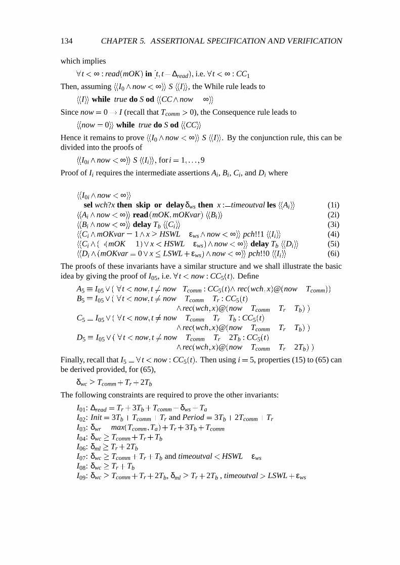
134 CHAPTER 5. ASSERTIONAL SPECIFICATION AND VERIFICATION
which implies
8t < ∞ : read(mOK) in [t; t+∆read); i.e. 8t < ∞ : CC1
Then, assuming hhI0^now < ∞ii S hhIii, the While rule leads to
hhIii while true do S od hhCC^now = ∞iiSince now = 0! I (recall that Tcomm > 0), the Consequence rule leads to
hhnow = 0ii while true do S od hhCCiiHence it remains to prove hhI0 ^now < ∞ii S hhIii. By the conjunction rule, this can bedivided into the proofs of
hhI0i^now < ∞ii S hhIiii; for i = 1; : : :;9
Proof of Ii requires the intermediate assertions Ai, Bi, Ci, and Di where
hhI0i^now < ∞iisel wch?x then skip or delayδws then x :=timeoutval les hhAiii (1i)hhAi ^now < ∞ii read(mOK;mOKvar) hhBiii (2i)hhBi ^now < ∞ii delay Tb hhCiii (3i)hhCi^mOKvar = 1^ x� HSWL� εws^now < ∞ii pch!!1 hhIiii (4i)hhCi^ (:(mOK = 1)_ x < HSWL� εws)^now < ∞ii delay Tb hhDiii (5i)hhDi^ (mOKvar = 0_ x� LSWL+ εws)^now < ∞ii pch!!0 hhIiii (6i)
The proofs of these invariants have a similar structure and we shall illustrate the basicidea by giving the proof of I05, i.e. 8 t < now : CC5(t). Define
A5 � I05_ ( 8t < now; t 6= now�Tcomm : CC5(t)^ rec(wch;x)@(now�Tcomm))B5 � I05_ ( 8t < now; t 6= now�Tcomm�Tr : CC5(t)
^ rec(wch;x)@(now�Tcomm�Tr�Tb) )C5 � I05_ ( 8t < now; t 6= now�Tcomm�Tr�Tb : CC5(t)
^ rec(wch;x)@(now�Tcomm�Tr�Tb) )D5 � I05_ ( 8 t < now; t 6= now�Tcomm�Tr�2Tb : CC5(t)
^ rec(wch;x)@(now�Tcomm�Tr�2Tb) )
Finally, recall that I5 �8 t < now : CC5(t). Then using i = 5, properties (15) to (65) canbe derived provided, for (65),
δwc � Tcomm+Tr +2Tb
The following constraints are required to prove the other invariants:
I01: ∆read = Tr +3Tb+Tcomm+δws +Ta
I02: Init = 3Tb+Tcomm+Tr and Period = 3Tb+2Tcomm+Tr
I03: δwr = max(Tcomm;Ta)+Tr +3Tb+Tcomm
I04: δwc � Tcomm+Tr +TbI06: δml � Tr +2TbI07: δwc � Tcomm+Tr +Tb and timeoutval < HSWL� εws
I08: δwc � Tr +TbI09: δwc � Tcomm+Tr +2Tb, δml � Tr +2Tb , timeoutval > LSWL+ εws

5.6. THE MINE PUMP EXAMPLE: FINAL IMPLEMENTATION 135
5.6.1 Conclusion: mine pump example
Finally, we can combine the design steps of the mine pump system and derive the con-straints that are needed to ensure correctness. The previous section showed a programwhich correctly implements MContr with
∆read = Tr +3Tb+Tcomm+δws +Ta
Init = 3Tb+Tcomm+Tr
Period= 3Tb+2Tcomm+Tr
δwr = max(Tcomm;Ta)+Tr +3Tb+Tcomm
δwc = Tcomm+Tr +2Tbδml = Tr +2Tb
and provided
LSWL+ εws < timeoutval < HSWL� εws
The design steps of preceding sections were proved to be correct, provided the followingheld:
� For Lemma 5.3, LSWL� LWL+δsc λmaxout , HSWL� HWL�δsc λmax
in
and λmaxin < λmin
out .� For Lemma 5.8, δsc � δpc+δp.� For Lemma 5.9, δpc � δws +δwr +δwc.� For Lemma 5.10, (∆read +δml +δp)λmax
ml � CML�SML.� For Lemma 5.11, LSWL� εws < HSWL+ εws.
These can be combined into the following list of constraints:
LSWL+2εws < HSWL
LSWL � LWL+(δws +δwr +δwc+δp)λmaxout
HSWL � HWL� (δws +δwr +δwc+δp)λmaxin
λmaxin < λmin
out
(∆read+δml +δp)λmaxml � CML�SML
To represent the reaction time we define an auxiliary parameter
∆react= δws +δwr +δwc+δp
= δws +δp+max(Tcomm;Ta)+2Tr +5Tb+2Tcomm:
To satisfy these requirements, define
LSWL = LWL+∆react λmaxout (5.13)
HSWL = HWL�∆react λmaxin (5.14)
SML = CML� (∆read+δml +δp)λmaxml (5.15)
= CML� (2Tr +5Tb+Tcomm+Taδws +δp)λmaxml (5.16)

136 CHAPTER 5. ASSERTIONAL SPECIFICATION AND VERIFICATION
Note that the constraint LSWL+2εws < HSWL then corresponds to
LWL+∆react λmaxout +2εws < HWL�∆react λmax
in
Combining the constraints leads to the correctness of
hhnow = 0ii SumpkPumpkWSenskAir kMSenskMContr hhCTLiiprovided
λmaxin < λmin
out
LWL+∆react(λmaxout +λmax
in )+2εws < HWL
where MContr is the program given at the start of this section, with timeoutval such thatLSWL + εws < timeoutval < HSWL� εws (note that by (5.13) such a value exists) andgiven the specifications of:
� Sump with LSWL and HSWL and a given maximum inflow λmaxin ,
� Pump with Init = 3Tb+Tcomm+Tr, Period = 3Tb+2Tcomm+Tr and given valuesof δp and minimal outflow λmin
out ,� WSens for given values of δws and εws,� Air for a given value of λmax
ml and with SML as defined above,� MSens with SML as defined above.
5.7 Further work
The proof system described in this chapter can be extended and used in different ways.We shall consider briefly a few of these: scheduling, protocol verification and mechanicalverification.
5.7.1 Scheduling
With maximal parallelism, each process has its own processor. This model can be gener-alized to multi-programming where several processes share a one processor and schedul-ing is based on priorities. Execution on a single processor is modelled as an interleavingof the atomic actions of the processes assigned to it. This interleaving can be restrictedby the programmer by assigning priorities to statements. Then a processor only startsthe execution of a statement when no other statement with a higher priority is ready toexecute. In this extended formalism, the correctness of a program is based on a fixed(priority-based) scheduling algorithm (Hooman, 1991).
It might, however, be more convenient to have an intermediate level between schedul-ing theory and formal top-down system design in which the scheduling strategy is not yetfixed but requirements on the scheduler are specified. For instance, the implementationof the mine pump control system can be split into two parts. First we derive a set of taskswith periods and deadlines of the form

5.7. FURTHER WORK 137
schedule ( wch?x ) with period 2 [0;δws]schedule ( read(mOK;mOKvar) ) with period 2 [0;∆read]schedule ( T ) with period 2 [∆1;∆2] deadline 2 [0;∆3]where T � if mOKvar = 1^ x� HSWL� εws then pch!!1
else if mOKvar = 0_ x� LSWL+ εws then pch!!0 fi fi
Scheduling theory (see Chapters 3 and 4) can then be used to construct a feasible schedulefor these tasks.
Alternatively, timing requirements can be specified explicitly by annotating programswith timing expressions (as was done in the Dedos project (Hammer et al., 1994)). Noassumptions are made about the execution time of statements but with the timing annota-tions requirements can be expressed for the execution time of statements. It is then left toa scheduler to guarantee that these timing requirements are satisfied. The formalizationof this approach is a topic of current research.
5.7.2 Protocol verification
In Hooman (1993; 1994a), a distributed real-time arbitration protocol based on an algo-rithm of the IEEE 896 Futurebus specification (IEEE, 1988) for networks of processesP1k � � �kPn using a general strategy:
1. Formulate a top-level specification for the network P1k � � �kPn, sayhhAii P1k � � �kPn hhCii
2. Axiomatize the communication mechanism between the processes P1; : : :;Pn byan axiom COMAX.
3. Find a suitable specification for each process Pi, for i = 1; : : :;n,hhAiii Pi hhCiii
in terms of the external communication interface of Pi only.4. Prove A! A1^ : : :^An and Comb(C1; : : :;Cn)^COMAX!C.5. Derive a correct implementation of process Pi, for i = 1; : : :;n, using the proof
method extended with rules for domain specific programming constructs.
This allows the development of a distributed program which satisfies the top-level speci-fication. In Step 4, the protocol is verified at an abstract level using the compositionalityof the parallel composition rule. Similar verification could be performed in another logic,e.g. a real-time version of temporal logic (Abadi & Lamport, 1994) or the duration cal-culus (Zhou et al., 1991a) (see Chapter 7). The triples find use in Step 5, where theirstructure is very convenient for the formal derivation of programs.
Step 2 requires the communication mechanism to be axiomatized. For this, the as-sertion language is extended with suitable primitives (e.g. to denote send and receiveactions) and the proof system is given axioms for these primitives (such as the relationbetween send and receive actions) and rules to relate communication statements of theprogramming language to the corresponding primitives of the assertion language.

138 CHAPTER 5. ASSERTIONAL SPECIFICATION AND VERIFICATION
Zhou and Hooman (1995) apply the first four steps of the method mentioned aboveto an atomic broadcast protocol (Cristian et al., 1989) which requires timing correctnessand fault-tolerance. The reliability of real-time systems requires the use of techniquesthat ensure the correct functioning of the system despite failures in some components.But providing such fault-tolerance usually influences the timing behaviour of a system.Given this strong relation between real-time and fault-tolerance, it would be desirable toextend our real-time framework to deal with fault-tolerance (see Chapter 8).
5.7.3 Mechanized support
Most of the work mentioned here has been based on manual, deductive verification but itis obvious that for a system of reasonable size some mechanized tool support is essential.This would allow proofs to be constructed interactively and checked mechanically so thatsimple verification conditions can be discharged automatically.
The Prototype Verification System PVS (Owre et al., 1992) has been used to verify de-sign steps during top-down design in the assumption–commitment framework presentedin this chapter. The PVS specification language is a strongly typed higher-order logic.Specifications are structured into a hierarchy of parameterized ‘theories’ and some theo-ries are built-in (e.g., reals, lists, sets, ordering relations, etc.). There is a mechanism toautomatically generate theories for abstract data types. The PVS system has an interac-tive proof checker with induction rules, automatic rewriting and decision procedures forarithmetic. PVS proof steps can be composed into proof strategies.
To use the PVS specification language, a slight reformulation (Hooman, 1994b) wasmade in the framework to obtain a mixed formalism in which programs and specifica-tions are unified (similar to, e.g. the mixed terms of Olderog (1985) and Zwiers (Zwiers,1989)). In such a framework, assertional specifications can be freely mixed with con-structs from the programming language. This makes it possible to formalize the processof program design and to describe the intermediate stages.
Use of this tool was demonstrated for the top-down derivation of a distributed real-timecontrol system (a chemical batch processing system). Simple details are proved automat-ically using the PVS decision procedures. This improves the speed of the design and theverification and allows the user to concentrate on the essential structure of proofs. Fur-ther, the possibility of building hierarchies of parameterized theories is also very useful.
5.8 Historical background
5.8.1 Semantics
The programming language of this chapter and its semantics are to a large extent influ-enced by the work of Koymans et al. (1988) who defined a denotational real-time seman-tics for the maximal parallelism model. In Huizing et al. (1987), a fully abstract version
5.8. HISTORICAL BACKGROUND 139
of this semantics was developed. These semantic models are based on the linear historysemantics of Francez et al. (1984).
The approach was extended to communicating shared resources by Gerber and Lee(1989; 1990). To obtain a calculus for shared resources a priority-based process algebrawas presented. The computation model was defined by an operational semantics in whichpriorities are not taken into account but were incorporated later using an equivalence.Global, discrete time is obtained by assuming that all actions take one time unit.
An alternative, topological, approach can be found in Reed and Roscoe (1986), wherethe real-time behaviour of CSP programs is defined by means of complete metric spaces(see Chapter 6).
5.8.2 Hoare logic
Our formalism is based on classical Hoare triples (Hoare, 1969). These correctness for-mulae have been used for the specification and verification of many non-real-time pro-gramming languages. A good survey was given by Apt (1981; 1984) and an extensiveformal treatment can be found in de Bakker (1980).
Usually, verification methods such as that by Manna and Pnueli (1982) for temporallogic and others by Owicki and Gries (1976), Apt et al. (1980) and Levin and Gries(1981) for the verification of parallel programs using Hoare triples, require the completeprogram text to be available. In contrast with these methods, we have formulated com-positional proof systems which allow reasoning with the specifications of componentswithout knowing their implementation. Compositionality can be considered to be a pre-requisite for hierarchical, structured program derivation. A separation of concerns is thenpossible between the use of (and the reasoning about) a module and its implementation(Dijkstra, 1976; Lamport, 1983). With a compositional proof system, design steps canbe verified during the process of top-down program construction. An overview of thetransition from non-compositional proof methods towards compositional proof systemscan be found de Roever (1985) and Hooman and de Roever (1986; 1990). The compo-sitional proof system for our modified Hoare triples was inspired by the work of Zwiers(1989) and preliminary accounts can be found in Hooman (1987; 1990; 1991).
Related work was done by Haase (1981) who introduced real-time as a variable in thedata space of the program and derived assertions using Dijkstra’s weakest preconditioncalculus (Dijkstra, 1976). Bernstein (1987) discusses several ways of modelling messagepassing with time-out in the non-compositional framework of Levin and Gries (1981).A non-compositional approach can be found in Schneider et al. (1992), where a logicof proof outlines with control predicates is extended to concurrent real-time programsby adding a primitive to express the time at which a control predicate last became true.A similar extension of Hoare Logic was given by Shankar (1993) using a more generalprimitive to express the time that has elapsed since an assertion last held.
PVS (Owre et al., 1992) and its predecessor, EHDM, have been used for a number ofapplications. EHDM was used to model digital flight-control systems (Rushby, 1993),for proof of an interactive convergence clock synchronization algorithm (Rushby & von

140 CHAPTER 5. ASSERTIONAL SPECIFICATION AND VERIFICATION
Henke, 1993) and Byzantine fault-tolerant clock synchronization (Shankar, 1993). Anapplication of PVS was described by Lincoln and Rushby (1993), where an algorithmfor interactive consistency has been verified.
5.8.3 Related work
Traditional linear time temporal logic (Pnueli, 1977; Manna & Pnueli, 1982; Owicki &Lamport, 1982) has been shown to be valuable in the specification and verification ofthe non-real-time behaviour of programs. It allows the expression of safety and live-ness properties by using a qualitative notion of time. For instance, for an assertion ϕ,this logic can express the safety property ‘henceforth ϕ will hold’ (2ϕ) and the livenessproperty ‘eventually ϕ will hold’ (3ϕ). To specify real-time constraints, a quantitativenotion of time has to be introduced. As already observed (Pnueli & Harel, 1988; Harelet al., 1990), there are two main approaches to defining real-time versions of temporallogic. In the first, this logic is extended with a special variable which explicitly refersto the value of a global clock, the so-called Explicit Clock Temporal Logic. Descrip-tions of non-compositional proof methods using Explicit Clock Temporal Logic basedon Manna and Pnueli (1982), can be found in Harel (1988) and Ostroff (1989), wheredecision procedures for this logic are given. A compositional proof method using Ex-plicit Clock Temporal Logic was formulated by Hooman et al. (1991).
An alternative approach uses an extension proposed by Koymans et al. (1983) andKoymans and de Roever (1985), in which the scope of temporal operators is restricted byusing time-bounds. Then we can express, for instance, ‘during the next seven time units ϕwill hold’ (2<7 ϕ) and ‘eventually within five time units ϕ will hold’ (3<5 ϕ). This logicis called Metric Temporal Logic (MTL), since in general it extends temporal logic by ametric point structure with a distance function to measure time; Koymans (1990; 1992)has a detailed discussion on MTL and several examples to illustrate its application to thespecification of real-time systems. An early use of temporal operators with time-boundscan be found in Bernstein and Harter (1981), where a quantitative ‘leads to’ operator wasintroduced to verify real-time applications. In Koymans et al. (1983) a version of MTLwas applied to the specification of real-time communication properties of a transmissionmedium. A temporal logic with statements about time intervals has been used by Shashaet al. (1984) to prove the correctness of local area network protocols. Hooman (1991)formulated a compositional proof system for formulae of the form S sat ϕ, where S is aprogram and ϕ a (real-time) property expressed in MTL. This proof system is based oncompositional proof methods for classical temporal logic (Barringer et al., 1984; Nguyenet al., 1986) and a preliminary version, for a simplified language, appeared in Hoomanand Widom (1989).
Logics for reasoning about real-time systems were classified by Alur and Henzinger(1990) according to their complexity and expressiveness. A tableau-based decision pro-cedure is given for a version of metric temporal logic. For decidability, a discrete timedomain is used. In a decidable version of the explicit clock approach (called TPTL),special variables represent values of a global clock and a ‘freezing’ quantification binds
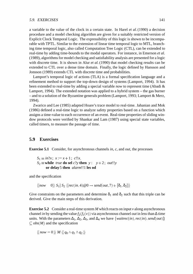
5.9. EXERCISES 141
a variable to the value of the clock in a certain state. In Harel et al. (1990) a decisionprocedure and a model checking algorithm are given for a suitably restricted version ofExplicit Clock Temporal Logic. The expressibility of this logic is shown to be incompa-rable with TPTL. Similar to the extension of linear time temporal logic to MTL, branch-ing time temporal logic, also called Computation Tree Logic (CTL), can be extended toreal-time by adding time-bounds to the modal operators. For instance, in Emerson et al.(1989), algorithms for model checking and satisfiability analysis are presented for a logicwith discrete time. It is shown in Alur et al. (1990) that model checking results can beextended to CTL over a dense time domain. Finally, the logic defined by Hansson andJonsson (1989) extends CTL with discrete time and probabilities.
Lamport’s temporal logic of actions (TLA) is a formal specification language and arefinement method to support the top-down design of systems (Lamport, 1994). It hasbeen extended to real-time by adding a special variable now to represent time (Abadi &Lamport, 1994). The extended notation was applied to a hybrid system – the gas burner– and to a solution of the Byzantine generals problem (Lamport, 1993; Lamport & Merz,1994).
Zwarico and Lee (1985) adapted Hoare’s trace model to real-time. Jahanian and Mok(1986) defined a real-time logic to analyze safety properties based on a function whichassigns a time-value to each occurrence of an event. Real-time properties of sliding win-dow protocols were verified by Shankar and Lam (1987) using special state variables,called timers, to measure the passage of time.
5.9 Exercises
Exercise 5.1 Consider, for asynchronous channels in, c, and out, the processes
S1 � in?x ; x := x+1 ; c!!x;S2 �while true do sel c?y then y := y+2 ; out!!y
or delay5 then alarm!!1 les od
and the specification
hhnow = 0ii S1kS2 hhrec(in;4)@0! send(out;7) 2 [δ1;δ2]ii
Give constraints on the parameters and determine δ1 and δ2 such that this triple can bederived. Give the main steps of this derivation.
Exercise 5.2 Consider a real-time system M which reacts on input v along asynchronouschannel in by sending the value f2(f1(v)) via asynchronous channel out in less than ∆ timeunits. With the parameters ∆1, ∆2, ∆3, and ∆4 we have fwaitrec(in); rec(in); send(out)g� obs(M) and the specification
hhnow = 0 ii M hhq0^q1^q2 ii

142 CHAPTER 5. ASSERTIONAL SPECIFICATION AND VERIFICATION
where
q0 � maxsend(out;∆1;∆2) during [0;∞)
q1 � minwait(in;∆3;∆4) during [0;∞)
q2 � 8t < ∞ : rec(in;v)@t! send(out; f2(f1(v))) in [t; t+∆)
(a) Suppose we have an environment E with
fsend(in);waitrec(out); rec(out)g � obs(E)
satisfying
hhnow = 0 ii E hh r1 ^ r2iiwhere
r1 � maxsend(in;∆3;∆4) during [0;∞)
r2 � minwait(out;∆1;∆2) during [0;∞):
Prove
hhnow = 0 ii MkE hhq iiwith q� 8t < ∞ : send(in;v)@t! rec(out; f2(f1(v))) in [t; t+∆).
(b) Implement M by two parallel components M1 and M2 which compute f1 and f2,respectively, and communicate internally via the asynchronous channel mid. Com-ponent M1 is given by fwaitrec(in); rec(in); send(mid)g � obs(M1) and
hhnow = 0 ii M1 hhq1^q3 iiwhere q3 �8 t < ∞ : rec(in;v)@t! send(mid; f1(v))@(t+δ1). M2 is specified asfwaitrec(mid); rec(mid); send(out)g � obs(M2) and
hhnow = 0 ii M2 hhq0^q4^q5 iiwhere
q4 � 8t < ∞ : await rec(mid) in [t; t+δ2)
q5 � 8t < ∞ : (mid;v0)@t! send(out; f2(v0)) in [t; t+δ3)
Prove, under certain requirements on the parameters δ1, δ2, δ3 and ∆, that
hhnow = 0 ii M1kM2 hhq0^q1^q2 ii(c) Construct programs that satisfy the specifications of M1 and M2 and formulatethe required constraints on the parameters.
Exercise 5.3 Consider an asynchronous channel c and a parameter T 2 TIME. Provethe following implication:

5.9. EXERCISES 143
(9 t0 : waitrec(c) during [0; t0)^ (rec(c)@t0_ t0 = T))^ (9 t1 < T : :send(c) during [0; t1)^ send(c;v)@t1)! rec(c;v) in [0;T)
(Informally this says that if a process waits to receive input on c until either a message hasbeen received or time T has been reached, and if another process sends v along c beforeT, then v is received along c in less than T time units.)
Exercise 5.4 Consider the program S1kS2 with asynchronous channels in, mid, out andalarm. For S1 we have obs(S1) = fwaitrec(in); rec(in); send(mid)g and
hhnow = 0ii S1 hhq1iiwith
q1 � 8t < ∞ : rec(in;v)@t!9 t1 < 10 : :send(mid) during [0; t1)^ send(mid;v+1)@t1
S2 is specified by obs(S2) = fwaitrec(mid); rec(mid); send(out); send(alarm)g and
hhnow = 0ii S2 hhq2 ^q3^q4iiwith
q2 � 8t < ∞ : rec(mid;v)@t! send(out;v+2) in [t; t+25)
q3 � 9 t0 : waitrec(mid) during [0; t0)^ (rec(mid)@t0_ t0 = 10)and
q4 � waitrec(mid) during [0;0+10)! send(alarm)@10
(a) Prove that, under a certain condition on the parameter ∆,
hhnow = 0ii S1kS2 hhriiwith r� rec(in;v)@0! send(out;v+3) in [0;∆). Hint: use Exercise 5.3.
(b) Derive programs that satisfy the specifications of S1 and S2, given certain con-ditions on the parameters Ta, Tcomm, etc.
Exercise 5.5 Process P, specified below, used the asynchronous channels in, out andalarm:
fwaitrec(in); rec(in); send(out); send(alarm)g � obs(P)hhnow = 0ii P hhq1 ^q2^q3ii
with
q1 � 8t < ∞ : rec(in;v)@t! send(out; f (v)) in [t; t+2)q2 � 8t < ∞ : await rec(in) in [t; t+3)andq3 � 8t < ∞ : waitrec(in) during [t; t+10)! send(alarm) in [0; t+11)
Consider the following two possible specifications of the environment E of P:
(a) Suppose E satisfies the following specification:

144 CHAPTER 5. ASSERTIONAL SPECIFICATION AND VERIFICATION
����
Pn
re1
ren
W
P1
al
Figure 5.5 Watchdog timer network
fsend(in);waitrec(out); rec(out);waitrec(alarm); rec(alarm)g � obs(E)hhnow = 0ii E hhr1ii
with r1 � 8t < ∞ : send(in)@t! t� 3^ (:send(in)) during [t�3; t). Prove
hhnow = 0ii PkE hhq4iiwith q4 � 8t < ∞ : send(in;v)@t! send(out; f (v)) in [t; t+2).
(b) Now suppose E satisfies
fsend(in);waitrec(out); rec(out);waitrec(alarm); rec(alarm)g � obs(E)hhnow = 0ii E hhr2ii
where r2 � (:send(in)) during [4;17). Then prove
hhnow = 0ii PkE hhq5iiwhere q5 � send(alarm) in [0;18).
(c) Derive a program satisfying the specification of P, given certain conditions onthe parameters Ta, Tg, Tcomm, etc.
Exercise 5.6 Design a ‘watchdog’ process W whose job is to check whether the pro-cesses P1; : : :;Pn are functioning properly. The network is shown in Figure 5.5, wherere1; : : :; ren, and al are asynchronous channels.
Ignore the actual task to be performed by each Pi but assume that it is functioning cor-rectly iff it sends a reset signal to W on channel rei at least once every ten time units.As long as all processes Pi send a reset signal in time, the watchdog timer W does notcommunicate on the alarm channel al. But if W has to wait for a reset signal on a partic-ular rei for ten time units or more, it will send an alarm message on channel al within Ktime units. Ignore the behaviour of W after a communication on al. W can therefore bespecified by
hhnow = 0ii W hhCwiiwhere

5.9. EXERCISES 145
����
Wal
����
P1
Wn
W1
Pn
an
a1
re1
ren
Figure 5.6 Refinement of the watchdog timer network
Cw � 8t < ∞ :((9 i : waitrec(rei) during [t; t+10))!9 t0 < t+10+K : send(al)@t0)^(send(al)@t!9 i 2 f1; : : :;ng 9 t1 < ∞ : waitrec(rei) during [t1; t1+10))
(a) Prove that if each Pi sends a signal on channel rei at least once every ten timeunits then no signal is sent on al. To specify that the Pi are functioning properly,assume
hhnow = 0ii Pi hh8 t < ∞ : send(rei) in [t; t+10)ii
Then prove that an alarm message never occurs in the network, i.e.
hhnow = 0ii P1k � � �kPnkW hh:send(al) during [0;∞)ii
(By compositionality, the properties of the network P1k � � �kPnkW can be verifiedusing the specifications of the components, without knowing their implementa-tions.)
(b) Design a program to implement the watchdog process W and satisfy the com-mitment Cw. Since the reset signals of any of the processes P1; : : :;Pn may arriveat the same time, implement W as a parallel composition W �W1k � � �kWnkA (inFigure 5.6 the a1; : : :;an are synchronous channels). Process Wi is the watchdogfor Pi and signals process A via channel ai as soon as there is no communicationon rei for at least ten time units; process A waits for a signal on any of the ais; afterreceipt of a signal it sends a message on al.Since the exact timing requirements for Wi and A may not be clear at this level, useparameters Ki and Ka in their specifications. This leads to
hhnow = 0ii Wi hhCwi ii
where
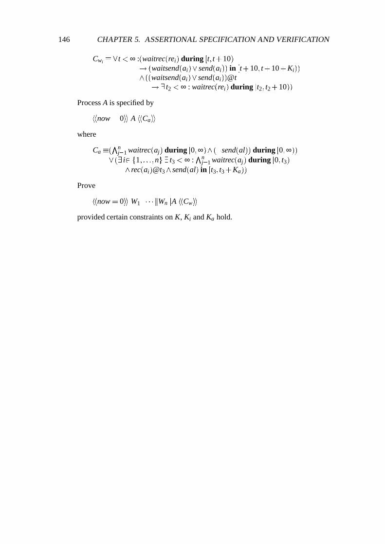
146 CHAPTER 5. ASSERTIONAL SPECIFICATION AND VERIFICATION
Cwi � 8t < ∞ :(waitrec(rei) during [t; t+10)! (waitsend(ai)_ send(ai)) in [t+10; t+10+Ki))^ ((waitsend(ai)_ send(ai))@t!9 t2 < ∞ : waitrec(rei) during [t2; t2+10))
Process A is specified by
hhnow = 0ii A hhCaiiwhere
Ca �(Vnj=1 waitrec(aj) during [0;∞)^ (:send(al)) during [0;∞))
_ (9 i2 f1; : : :;ng 9 t3 < ∞ :Vn
j=1 waitrec(aj) during [0; t3)^ rec(ai)@t3^ send(al) in [t3; t3+Ka))
Prove
hhnow = 0ii W1k � � �kWnkA hhCwiiprovided certain constraints on K, Ki and Ka hold.

Chapter 6
Specification and Verification in TimedCSP
Steve Schneider
Introduction
Communicating sequential processes (CSP) is a language designed to describe formallythe patterns of communication behaviour of system components or processes and howthese components may be combined. The theory of CSP enables the formal descriptionof system specifications and supports their analysis, judging them against the require-ments. A theory of refinement allows CSP descriptions at a high level of abstraction tobe refined to a level of description more appropriate for implementation. This allows ab-stract CSP processes to act as specifications, describing the behaviour expected of anyimplementation.
Timed CSP is a direct extension of the original CSP, and includes explicit timing con-structs enabling the description of quantitative timing behaviour. A theory of timewiserefinement allows mappings between untimed and timed processes. We will use the ab-breviation CSP to refer to the timed extension of the language.1
6.1 The language of real-time CSP
The CSP language describes processes in terms of their communication behaviour, re-moving internal state information that does not affect the communication behaviour. Thisabstraction is appropriate for real-time systems since they are reactive and interact contin-ually with their environment. The requirements of such systems are concerned primarilywith the interactions between a component and its environment.
1The reader should be aware that this is not the usual practice: the timed language is more commonlycalled real-time CSP.
147

148 CHAPTER 6. SPECIFICATION AND VERIFICATION IN TIMED CSP
6.1.1 Events and processes
A process is modelled in terms of the possible interactions it can have with its environ-ment, which may be thought of as another process or set of processes, the ‘outside world’,or a combination of these. The first step in the description of a process is to decide onthe ways in which interactions can take place.
Interactions are described in terms of instantaneous atomic synchronizations, orevents. This kind of synchronization is sufficiently simple to model asynchronous andshared memory communication. A process cooperating with its environment for somelength of time is described in terms of a single event occurring at the point at which theyagree to cooperate. A process can be considered as a ‘black box’ with an interface con-taining a number of events through which it interacts with other processes. The set of allevents in the interface of a process is called its alphabet. In this set, interface events aretreated as synchronizations between the participating processes and not as autonomousactions under the control of a single process. A process containing an event in its in-terface is required to participate in the occurrence of that event. The refusal of a singleparticipant to cooperate will block its occurrence.
6.1.2 Computational model
Before we formally describe the language of CSP and how it is to be understood, we mustmake explicit a number of assumptions concerning the underlying model of computationand the nature of time:
� Maximal progress: A synchronization event occurs as soon as all participants areready to perform it.
� Maximal parallelism: Every process has a dedicated processor; processes do notcompete for processor time.
� Finite variability: No process may perform infinitely many events, or undergo in-finitely many state changes, in a finite interval of time.
� Real-time: The time domain is taken to be the non-negative real numbers. Thusit is possible for events to occur at any non-negative real time. Since the reals aredense, our maximal parallelism assumption above means that there is no positivelower bound on the time difference between two independent events occurring atdifferent times.
� Newtonian time: Time progresses in all processes at the same rate, and all withrespect to the same unique global time frame.
The assumption of maximal progress has close connections with the treatment of pro-cesses and the events that they may perform. In addition to the events in the interface ofa process (external events), a process description may also include internal events. Theinterface of a process P will not contain its internal events as they will be performed by P

6.1. THE LANGUAGE OF REAL-TIME CSP 149
without the participation of its environment. In practice, an internal event usually corre-sponds to a synchronization between parallel components of P. Maximal progress meansthat an internal event occurs as soon as P is ready to perform it, and this will be as soonas all the participating components of P are ready.
External events, on the other hand, require the participation of the environment of P.An external event a can occur only when all processes which contain a in their interfaceagree to perform it. If P is one of a number of such processes which are components ofa composite process R, and the event a is external for R, then the occurrence of a willbe influenced by R’s environment. If a is internal to R, then by maximal progress it willoccur as soon as all the participants, one of which is P, are able to perform it.
6.1.3 The operators of CSP
The language of CSP is defined by the following pseudo Backus–Naur form definitions:
P ::= STOP j SKIP j P; P j a! P j sequential
P 2 P j P u P j P t. P j choice
P j[A jA ]j P j P jjj P j parallel
P n A j f (P) j f�1(P) j abstraction
X j µX � P recursion
Σ is the set of all possible events, a is in Σ, A in P (Σ), t in [0;∞), f is a function Σ! Σand X is a process variable. CSP processes are terms with no free process variables (i.e.every process variable is bound by some µ expression). In a CSP process, every recursiveexpression is time-guarded to ensure finite variability (i.e. there is some t > 0 for whichany execution must take at least t to reach a recursive invocation). Since the only operator
that introduces a delay is the timeout operatort., every occurrence of a process variable
must be guarded by a non-zero timeout.We shall use the convention that events are written in lower case, and processes are
written in upper case.
SequentialThe process STOP is the deadlocked process, unable to engage in any events or makeany progress (this might adequately describe a surly waiter in a restaurant who refuses toserve any customer). It might be used to describe a system which has crashed, or whichhas deadlocked: no further events are possible.
The process SKIP is the immediately terminating process. This might describe thewaiter whose shift ends as soon as it starts. No events are performed, but in contrast toSTOP it can signal to its environment that it has terminated, and an appropriate environ-ment would be able to pass control to another process.
The sequential composition P; Q behaves as P until P terminates, and then behaves asQ. Thus WAITER1; WAITER2 initially behaves as WAITER1 until the shift finishes; the

150 CHAPTER 6. SPECIFICATION AND VERIFICATION IN TIMED CSP
subsequent behaviour is that of WAITER2.As we might expect, SKIP; P =P for any P, and STOP; P = STOP; indeed the seman-
tic model supports these equations. The first equation states that since SKIP does nothingexcept immediately pass control to P, the resulting behaviour is indistinguishable fromthat of P. In the second equation, the deadlocked process STOP does not indicate termi-nation so P will never be reached and the result is equivalent to STOP.
The prefix process a! P is ready to engage in event a (and in no other event). It willcontinue to wait until its environment is also ready to perform a, at which point synchro-nization on this event will occur. Once the event is performed, the subsequent behaviourof a! P will be that of process P. By default, there is no delay between the occurrenceof a and the beginning of P. A waiter who is prepared to take a customer’s coat beforeserving may be described by the process coat! SERVE, where the event coat modelsthe synchronization between customer and waiter achieved by the removal of the coat.
We later define a form of prefix which explicitly introduces a delay: at!P is also ready
initially to engage in a; but once that event is performed, there is a delay of t before itbehaves as P. The waiter who takes ten minutes between removing the coat and serving
would be described by coat10! SERVE.
The behaviour of a waiter to a single customer may be described by the following pro-cess:
WAITER = table2! coat
5! order20! serve
30!pay
0:01! tip3! coat! SKIP
The waiter is prepared to show a customer to a table, then, after a short delay, to removea coat, then take an order, serve, accept payment, accept a tip and finally return the coat.Observe that each of these events indicates a readiness to interact: if the customer is notready to order until ten minutes after the coat is taken, the waiter will wait; if the customeris ready after only three minutes, the waiter will not yet be ready to interact.
ChoiceAn external choice P2 Q is initially ready to engage in events that either P or Q is readyto engage in. The first event performed resolves the choice in favour of the componentthat was able to perform it, and the subsequent behaviour is given by this component.
A choice offered to the customer between two items on the menu could be modelledusing this choice:
duck20! SERVEd 2 grouse
20! SERVEg
Here, a choice of two processes, duck20! SERVEd and grouse
20! SERVEg , is offered tothe customer. Both initial events are available, and the choice is resolved at the point thecustomer performs one of these events.
An internal choice P u Q behaves either as P or as Q but, unlike the external choice,the environment cannot influence the way the choice is resolved. The choice
duck20! SERVEd u grouse
20! SERVEg

6.1. THE LANGUAGE OF REAL-TIME CSP 151
is not made by the customer, but is made instead by the system (the restaurant in thiscase), and the customer has no influence over which way it is resolved. It may be resolvedby always choosing duck, by tossing a coin, by alternating between duck and grouse or bychoosing whichever is cheaper. Any of these approaches will be acceptable to a customerwho does not mind which of the items is eventually served, as long as at least one of duckor grouse is offered.
The timeout choice Pt. Q initially behaves as process P. If an event is performed be-
fore time t, then the choice is resolved in favour of P, which continues to execute, andQ is discarded. If no such event is performed, then the timeout occurs at time t, and thesubsequent behaviour is that of Q. An impatient customer may wait five minutes for atable, but will leave the restaurant if no table becomes available in that time. This may
be described by the process CUST = (table!MEAL)5. LEAVE. If the event table is not
performed within five units of time (minutes in this case), then the timeout will occur,since the first process will not have performed any events, and the customer will behaveas the exception process.
Timeout may be used to handle exceptions in a number of ways. It may provide op-portunities for disagreement. The following fragment from the wedding service providesan illustration:
(speak now! DISRUPTION)10. FOREVER HOLD PEACE
The expectation is that the timeout should occur (i.e. that the event speak now does notoccur), but an opportunity should be provided to prevent it if necessary.
More often, timeout is used to detect errors: if an expected response is not receivedwithin a certain time, some corrective action should be taken.
ParallelThe parallel combination P j[A jB ]j Q allows P to engage in events from the set A (only),and Q to engage in events from the set B (only). The processes P and Q must synchro-nize on all events in the intersection A\B of these two interfaces, but other events areperformed independently.
The customer CUST may have a set of possible interactions:
AC = ftable;order; serve;eat;pay; tip;coatgAlthough any real customer will have other actions of interest, we are interested in mod-elling interactions with the restaurant, and so we have abstracted all activity irrelevant tothe situation we are modelling.
Events of interest in the restaurant might be described by the set
AR = ftable;order;pay; tip;coat; serve;cookgA waiter who has a table ready will be able to interact with the customer:
CUST j[AC jAR ]j WAITER

152 CHAPTER 6. SPECIFICATION AND VERIFICATION IN TIMED CSP
But, a waiter who has a cigarette before showing a customer to a table may lose the cus-tomer:
CUST j[AC jAR ]j CIGARETTE; WAITER
If CIGARETTE takes too long to terminate, the customer may no longer wish to be shownto a table but if it terminates sufficiently quickly, the waiter will be ready before the cus-tomer walks out. The event table can occur only at times when both participants are pre-pared to engage in it.
If the process MEAL is eat15! coat! SKIP, then the customer CUST (defined in terms
of MEAL) is not prepared to offer a tip and requires the return of his coat after eating.Since the waiter is not prepared to return the coat until a tip has been received, the parallelcombination of CUST with WAITER will deadlock: although each participant is able tocontinue on some event, there is no event on which they can they can agree.
The asynchronous parallel combination P jjjQ represents the independent concurrentexecution of P and Q, with no synchronization between them on any events. A numberof separate waiters might be described using this construct:
WAITERS = WAITER jjjWAITER jjj : : : jjjWAITER
None of the waiters interacts with any other, though they may all interact with a customer.In the combination
CUST j[AC jAR ]j WAITERS
the customer can cooperate with any waiter; the choice between waiters is nondetermin-istic: any that is prepared to perform table when the customer performs it may be chosen.
AbstractionThe hiding operator P n A makes the events in the set A internal to the process, thus re-moving them from the control of the environment. The only participants will then be thecomponents of P. From the maximal progress assumption, the internal events will occuras soon as P is ready to perform them. In general, internal events occur as soon as theyare ready, unless they are pre-empted because of conflict, such as when there is a choicebetween events.
A print spooler SPOOL and PRINTER communicate via channel print:
SPOOL = in2! print
3! SPOOL
PRINTER = print30! out! PRINTER
The parallel combination SPOOL j[ in;print jprint;out ]j PRINTER has print as a visiblechannel and further processes may participate in it. Since only SPOOL and PRINTERshould participate in that synchronization, we make print internal:
(SPOOL j[ in;print jprint;out ]j PRINTER) n print

6.1. THE LANGUAGE OF REAL-TIME CSP 153
and the event print will occur as soon as both processes are ready to perform it.The renaming operators f (P) and f�1(P) change the names of events through the al-
phabet mapping function f . This allows a generic pattern of communication to be definedfor use with different events. For example, a waiter responsible for table i might be de-scribed by a generic WAITER process and a renaming fi which maps any event a to ai.Thus f1(WAITER) is prepared to show a customer to table 1, but to no other table.
Renaming using the inverse function f�1 allows a number of events to trigger a partic-ular communication. If function g has g(credit card) = pay and g(cash) = pay, then theprocess g�1(WAITER) is prepared to engage in a credit card event or a cash event when-ever WAITER is prepared to accept a pay event. The function h satisfying h(tablei) =table allows h�1(WAITER) to show a customer to any table:
g�1(WAITER) = table2! coat
5! order20! serve
30!(credit card
0:01! tip3! coat! SKIP
2 cash0:01! tip
3! coat! SKIP)
h�1(WAITER) = (table12! coat
5! order20! serve
30!credit card
0:01! tip3! coat! SKIP)
2 (table22! coat
5! order20! serve
30!credit card
0:01! tip3! coat! SKIP)
...
2 (tablen2! coat
5! order20! serve
30!credit card
0:01! tip3! coat! SKIP)
RecursionA recursive term µX � P behaves as P, with every occurrence of X in P representing animmediate recursive invocation. Thus we will have the usual law
µX � P = P[µX � P=X]
Every recursive term of the form µX � P that has P must be t-guarded for X for somet > 0 — so that every occurrence of X in P requires the passage of at least t units of timebefore it can be reached.
A waiter who deals with customers repeatedly may be described by the recursive pro-cess µX �WAITER; X, or alternatively by a recursive definition.
RWAITER = table2! coat
5! order20! serve
30!pay
0:01! tip3! coat! RWAITER

154 CHAPTER 6. SPECIFICATION AND VERIFICATION IN TIMED CSP
6.1.4 Generalized operators
The delay process Wait t is a timed form of SKIP which does nothing for t units of timeand then terminates successfully:
Wait t = STOPt. SKIP
The timeout choice will wait for t units of time, but the process STOP cannot performany event and at time t control is passed to SKIP, which then terminates immediately.
A delayed form of prefixing can be defined as
at! P = a! (Wait t; P)
After the event a, there is a delay of t before control reaches P.Generalizing choice to allow infinite choices is often useful. The prefix choice
a : A! Pa
remains willing to perform any event from set A until one is chosen. Its subsequent be-haviour, given by Pa, is dependent on that event. Thus a construct can be defined to allowthe input on channel in of any item x in a set M, and the value x determines the subsequentbehaviour:
in?x : M! Q(x) = a : in:M! Pa
where the set in:M = fin:m j m 2 Mg and Pin:m = Q(m) for every m 2 M. The atomicsynchronization events here are of the form in:m. The complement is the output prefixwhich has the form out!x! P and this is simply shorthand for out:x! P.
Thus a one-place delaying buffer might be described by the recursive process
DBUFFER = in?x1! out!x! DBUFFER
There is a one-second delay between in? and out!, but no delay is enforced between out!output and the subsequent in?.
Infinite nondeterministic choice may also be defined. The process uj2J
Pj for some
indexing set J may behave as any of its arguments Pj. Thus, for example, a nondeter-ministic delay over some interval I may be defined:
Wait I = ut2IWait t
The delay may be for any time in the interval I. If each Pi is t-guarded for X, then so istheir infinite choice and if P is t-guarded for X, then Wait I; P is (t+ infI)-guarded forX.
Alphabet parallel composition generalizes as expected. The processkAiPi gives inter-
face Ai to each process Pi. To perform an event a, all processes with a in their interfacemust participate.

6.1. THE LANGUAGE OF REAL-TIME CSP 155
A form of parallel composition which allows synchronization on some events and in-terleaving on others may be defined by the use of event renaming. Define
fA(x) = a:x if x 62 Ax otherwise
gA(x) = b:x if x 62 Ax otherwise
h(y) = x if y = a:x or y = b:xy otherwise
The process P j[A ]jQ synchronizes on events in A, and interleaves on all other events.
P j[A ]jQ = h(fA(P) j[A[a:Σ jA[b:Σ ]j gA(P))
If two runners are defined as
RUNNER1 = startt1! finish! STOP
RUNNER2 = startt2! finish! STOP
then a race between the two runners may be modelled as
RUNNER1 j[start ]jRUNNER2
They must both start at the same time (so they synchronize on start) but they may finishat different times.
Exercise 6.1.1 Write CSP processes which describe the following situations. Decidefirst which events are to be used (the alphabet of the process), and then provide a CSPdescription:
1. A vending machine which is initially ready to accept a coin, and is then alwaysready to accept a coin within two seconds of the last item being dispensed; and itoffers the customer the choice of a biscuit or a chocolate five seconds after insertionof a coin.Its interface will be the set of events fcoin;bisc;chocg.
2. A transmitter which sends a message every five seconds until an acknowledgementis received.
3. An oven with a timer set to T which rings after T minutes of being switched on, ifnot switched off beforehand.
4. A baby who wakes up nondeterministically between one and eight hours after go-ing to sleep.
5. A baby who needs to be rocked for five minutes to get to sleep. If rocking stopsbefore then, she cries; otherwise she sleeps.
6. A baby who starts to cry if not fed within two minutes of waking.7. A baby who has all of the above characteristics. (Hint: use a parallel combination
of the CSP processes you have already defined.)

156 CHAPTER 6. SPECIFICATION AND VERIFICATION IN TIMED CSP
6.2 Observations and processes
The language of CSP has a formal meaning and the behaviour of a CSP process is pre-cisely defined. This makes it possible to judge CSP descriptions against specificationswhich characterize desired behaviour. Such specifications may be written in a languageoriented towards expression of properties (such as temporal logic), or even as a CSP pro-cess which describes the desired behaviour.
6.2.1 Notation
Let Σ be the set of events, variables t and t0 represent times and range over R+ and vari-able s range over Traces, the finite and infinite sequences of timed events (t;a). We useℵ to range over sets of timed events in IRSET, the set of refusals, defined below.
The following operations will be used on sequences of events: #s is the length of thesequence s; s1
a s2 denotes the concatenation of s1 and s2. The beginning and end of asequence is defined as follows: begin(h(t;a)ias) = t, end(sah(t;a)i) = t, first(h(t;a)ias) = a, last(sa h(t;a)i) = a. The notation s1 4 s2 means that s1 is a subsequence of s2and s1 6 s2 means that s1 is a prefix of s2. The following projections on sequences aredefined by list comprehension, where
hf (x) j x s;P(x)iis the maximal subsequence of s whose elements all satisfy P, with f applied to each term:
s� t = h(t0;a) j (t0;a) s; t0 6 tis " I = h(t0;a) j (t0;a) s; t0 2 Iis # A = h(t0;a) j (t0;a) s;a 2 Ais� t = h(t0� t;a) j (t0;a) s; t0 > ti
The set of events occurring in a trace is extracted by a set comprehension:
σ(s) = fa j s # fag 6= higs� t is that part of the trace that occurs no later than time t and s " I is the part that occursduring interval I. s # A is the subsequence of the trace whose events occur in the set A.In s� t, the trace s is moved backward through t units of time (and truncated so no eventoccurs before time 0), and σ(s) is the set of events which occur in s.
There are similar projections on refusal sets:
ℵ� t = f(u;a) j (u;a) 2ℵ;u < tgℵ # A = f(u;a) j (u;a) 2ℵ;a 2 Agℵ� t = f(u� t;a) j (u;a) 2ℵ;u> tgσ(ℵ) = fa j (u;a) 2ℵg

6.2. OBSERVATIONS AND PROCESSES 157
ℵ � t is the set of events in ℵ occurring strictly before time t. ℵ # A is that part of ℵcontaining events from the set A and ℵ� t is the set ℵ moved backward through t unitsof time. σ(ℵ) is the set of events occurring at some time in ℵ.
6.2.2 Observations
The formal semantics of CSP is defined in terms of timed failures. Each timed failurecorresponds to a record of an execution of the system and consists of a timed trace anda timed refusal.
Any observation of an execution of a process must include a record of the events thatwere performed and the times at which they occurred. A timed trace is a finite sequenceof timed events from the set [0;∞)�Σ such that the times associated with events appearin non-decreasing order.
Traces :P(seqω(R+�Σ))
s 2 Traces,h(t1;a1); (t2;a2)i 4 s) t1 6 t2^#s = ∞) supft j h(t;a)i 4 sg= ∞
Real-time systems are reactive and it is important to know when a process is willing tointeract with its environment and when this is not possible. For deterministic systems,this information can be obtained from the trace but for nondeterministic systems the traceinformation is not sufficient. For example, the traces of
a! STOP and STOP u a! STOP
are the same but the first must always respond in an environment in which a is ready,whereas the second may refuse to respond.
We will therefore also record timed refusal information. A timed refusal contains theevents (with times) which the process refused to engage in during an execution. From theassumption of finite variability, only finitely many state changes are possible in a finitetime. Since a process will continue to refuse an event while it remains in the same state,a timed refusal can be considered as a step function from times to sets of events. Theset IRSET is the set of all such refusals. It is defined in terms of RSET, those sets whichrecord refusal information only for some finite time:
RSET : P(R+�Σ)IRSET :P(R+�Σ)
ℵ 2 RSET,9b1 : : :bn;e1 : : :en : R+; A1 : : :An :P(Σ) �
ℵ =Sn
1([bi;ei)�Ai)ℵ 2 IRSET,8t �ℵ\ [0; t)�Σ2 RSET

158 CHAPTER 6. SPECIFICATION AND VERIFICATION IN TIMED CSP
ab refusalc
- tracea b a
- time0 1 2 3 4 5
Figure 6.1 A timed observation
Refusal information at any particular time is considered to be subsequent to the eventsrecorded in the trace at that time. For example, in the process
a! STOP 2 b! STOP
the event b cannot be refused before any events have occurred. But when a occurs, thepossibility of b is withdrawn and so it may thereafter be refused. Thus the step functionmay be considered to be closed at the lower end of a step, and open at the upper end.Further, once a has occurred, it, too, may be refused from that instant onwards since nofurther copies of a are possible for the process. Thus a timed event may occur in both atimed trace and in a corresponding timed refusal.
A single observation will consist of a CSP timed failure, made up of a trace s2 Traces,and a refusal set ℵ 2 IRSET from the same execution. The trace and refusal are consid-ered to be a record of the behaviour of the process over all time, even if s and ℵ both endat some finite time. If (s;ℵ) is an observation of P, then P has some execution duringwhich the events in s were performed and the events in ℵ were refused. In contrast tothe untimed failures model for CSP, this refusal contains information concerning eventsthat were refused both during and after the performance of s, whereas an untimed refusalset contains only information after the end of the trace.
Figure 6.1 shows the first 5:5 seconds of one possible observation of the recursive pro-cess:
P = a! ( Wait 2; b! P2
Wait 5; c! STOP)
Initially, event c is refused over the interval [0;1). At time 1, event a occurs and furthercopies of it are refused over the interval [1;3). Event b is refused over the interval [2;3),occurs at time 3 and then further occurrences are refused until time 5. b’s refusals upto that time therefore consist of the interval [2;5), indicating that the occurrence of b attime 3 must have been at the instant it was made available. c is refused over the inter-val [3:5;5:5). During this refusal, another occurrence of a is observed, at time 4. The

6.2. OBSERVATIONS AND PROCESSES 159
diagram corresponds to the timed failure
(h(1;a); (3;b); (4;a)i; [1;3)�fag[ [2;5)�fbg[ [0;1)�fcg[ [3:5;5:5)�fcg)
The refusal set could also be written in the form of a step function:
(h(1;a); (3;b); (4;a)i; [0;1)�fcg[ [1;2)�fag[ [2;3)�fa;bg[ [3;3:5)�fbg[ [3:5;5)�fb;cg[ [5;5:5)�fcg)
The refusal information is not a complete record of everything the process could haverefused – for example, it could have also refused b over the interval [0;2) – but it maybe considered as a record of what the process refused in an environment which madeparticular offers.
The set of all possible observations is given by
OBS = TT� IRSET
Any pair (s;ℵ) is a possible observation of some execution, so OBS consists of all pairs.Processes are associated with subsets of OBS. The notation MTI denotes the space of allsuch subsets of OBS.
6.2.3 The semantic function
The semantic function
FTI : CSP ! MTI
is defined by giving an equation for each of the operators of the language.
FTI [[STOP]] b= f(hi;ℵ) jℵ 2 IRSETg
No event may ever be performed by the process STOP and any set of events may be re-fused at any time.
FTI [[SKIP]] b= f(hi;ℵ) jX 62 σ(ℵ)g[f(h(u;X)i;ℵ) jX 62 σ(ℵ � u)g
The special event X denotes termination in the semantics of processes but it is not anevent in syntactic CSP expressions. There are two possibilities for SKIP: either it hasnot yet terminated, in which case it cannot refuse to do so (though anything else maybe refused), or it has terminated at time u, in which case it may refuse anything aftertermination but could not have refusedX before u.

160 CHAPTER 6. SPECIFICATION AND VERIFICATION IN TIMED CSP
FTI [[P; Q]] b= f(s;ℵ) jX 62 σ(s) ^ (s;ℵ[ ([0;∞)�fXg)) 2 FTI [[P]]_
s = sPa sQ ^X 62 σ(sP)
^ (sQ;ℵ)�u 2 FTI [[Q]] ^ begin(sQ) > u
^ (sPa h(u;X)i;ℵ� u[ ([0;u)�fXg)) 2 FTI [[P]]g
There are two possibilities for an execution of a sequential composition P; Q: either itis an execution of P, in which case it must have refused to terminate throughout the ex-ecution, or it is some terminating execution of P followed by an execution of Q; again Pmust have refused to terminate throughout its execution until it actually did so.
FTI [[a! P]] b= f(hi;ℵ) j a 62 σ(ℵ)g[
f(h(u;a)ia s;ℵ) j a 62 σ(ℵ� u)^ (s;ℵ)�u 2 FTI [[P]]g
The prefix process a ! P is unable initially to refuse a, which is the first event it mustperform. Either a does not occur, in which case anything except a may be refused, or aoccurs at some time u, having previously not been refused, and the subsequent behaviouris that of P starting at time u rather than at time 0.
FTI [[P2 Q]] b= f(hi;ℵ) j (hi;ℵ) 2 FTI [[P]]\FTI [[Q]]g[f(s;ℵ) j s 6= hi ^ (s;ℵ) 2 FTI [[P]][FTI [[Q]]
^(hi;ℵ� begin(s)) 2 FTI [[P]]\FTI [[Q]]g
In an external choice P2Q, initial events are available from either process; events can berefused only if both processes are able to refuse them. Once the choice has been resolved(at the time of the first event) in favour of one of the processes, the subsequent behaviouris given by that process.
FTI [[P u Q]] b= FTI [[P]][FTI [[Q]]
An execution of an internal choice is an execution of one of the component processes.
FTI [[Pu. Q]] b= f(s;ℵ) j begin(s) 6 u ^ (s;ℵ) 2 FTI [[P]]g
[
f(s;ℵ) j begin(s) > u ^ (hi;ℵ� u) 2 FTI [[P]]^(s;ℵ)�u 2 FTI [[Q]]g
In an execution of a timeout process Pu. Q, either P performs its first event before time
u, in which case the execution is simply one of P, or no event occurs before time u, andthe timeout passes control to Q. In the second case, the refusal up to time u is governed

6.2. OBSERVATIONS AND PROCESSES 161
by P, and the behaviour after u is that of Q translated to start at time u instead of at time0.
FTI [[P j[A jB ]j Q]] b= f(s;ℵ) j 9ℵP;ℵQ �
ℵ # (A[B) = (ℵP # A)[ (ℵQ # B)^ s = s # (A[B)^ (s # A;ℵP) 2 FTI [[P]]^ (s # B;ℵQ) 2 FTI [[Q]] g
In the parallel combination P j[A jB ]j Q, the execution projected onto the set A is due toP, and that onto the set B is due to Q. Where A and B intersect, both P and Q must agreeon events in the trace, but if any of them refuses an event the combination will refuse it.
FTI [[P jjj Q]] b= f(s;ℵ) j 9sP; sQ � s 2 sP jjj sQ^ (sP;ℵ) 2 FTI [[P]]^ (sQ;ℵ) 2 FTI [[Q]]g
where sP jjj sQ is the set of timed traces consisting of an interleaving of sP and sQ: in aninterleaved combination, each event requires the participation of precisely one compo-nent so both processes must refuse an event for the combination to refuse it.
FTI [[P n A]] b= f(s n A;ℵ) j (s;ℵ[ ([0;∞)�A)) 2 FTI [[P]]g
In an encapsulated process P n A, the events in A are made internal to the process (theydo not appear in the trace) and no longer require the participation of the environment:they are autonomous events under the control of P. By the maximal progress assump-tion, this means they should occur as soon as they are enabled. This corresponds to thecondition that A should be refusible for P over the entire execution: if this were not thecase, then there would be some period during which an event from A was enabled buthad not occurred, violating maximal progress.
FTI [[f (P)]] b= f(f (s);ℵ) j (s; f�1(ℵ)) 2 FTI [[P]]g
FTI [[f�1(P)]] = f(s;ℵ) j (f (s); f (ℵ)) 2 FTI [[P]]g
Processes whose alphabets are renamed have similar behaviour, but the names of theevents are transformed by the renaming function f .
FTI [[ui2IPi]] b= [
i2I
FTI [[Pi]]
The possible executions of a general choice are those of its components.
FTI [[a : A! Pa]] = f(hi;ℵ) j A\σ(ℵ) = øg[f(h(u;a)ia s;ℵ) j
a 2 A ^ A\σ(ℵ � u) = ø^ (s;ℵ)� t 2 FTI [[P(a)]]g

162 CHAPTER 6. SPECIFICATION AND VERIFICATION IN TIMED CSP
An execution of a prefix choice a : A!Pa takes one of two forms: either no event occurs,in which case nothing in A may be refused, or some event a 2 A is chosen at some timeu, in which case no event in A may be refused before u, and the subsequent behaviour isthat of the chosen process Pa, translated through u time units.
The recursive process µX � P is a solution of the equation X =P; this is the fixed pointof the semantic mapping corresponding to P with the most timed failures. The fixed pointwill exist for time-guarded recursive equations. Recursive equations may be process def-initions: the equation P = F(P) defines P to be the process µX � F(X).
Exercise 6.2.1 Consider the process P = (a4! b! STOP)2 c! STOP. Which of the
following are failures of P?
1. (h(1;a)i;ø) 2. (h(3;b); (1;a)i;ø)3. (h(6;b); (1;a)i;ø) 4. (h(1;a); (3;b)i;ø)5. (h(1;a); (5;b)i;ø) 6. (h(1;a); (5;b); (6;c)i;ø)7. (h(6;c)i;ø) 8. (hi;ø)9. (hi; [0;1)�fbg) 10. (h(1;a)i; [0;1)�fbg)11. (h(1;a)i; (0;1)�fbg) 12. (h(1;a)i; [0;1)�fag)13. (h(1;a); (5;b)i; [0;10)�fcg) 14. (h(1;a); (5;b)i; [1;10)�fcg)15. (h(1;a); (5;b)i; [1;2)�fag) 16. (h(6;c)i; [0;4)�fbg)
Exercise 6.2.2 Give a single process which has all of the following behaviours:
(hi; [0;2)�fag[ [5;8)�fag)(h(3;a)i; [0;2)�fag)(h(1;b)i; [0;2)�fag)
Give a process which has both of the following behaviours:
(hi; [0;∞)�fag)(h(1;a)i;ø)
6.3 Specification
A specification is a predicate S on timed failures. It describes the behaviour required ofthe system. Process P meets specification S (written P sat S) if S holds for every timedfailure in the semantics of P:
P sat S(s;ℵ) , 8(s;ℵ) 2 FTI [[P]] � S(s;ℵ) (6.1)
For example, the following specification requires the first event observed to be start:
S(s;ℵ) = (s = hi _ first(s) = start)
In any execution, either no event is observed (the trace will be empty) or the first eventis start.

6.3. SPECIFICATION 163
The requirement that P performs ons and off s alternately is represented by the speci-fication
S(s;ℵ) = 8u6 s � 06 #(s # on)�#(s # off )6 1
In every prefix of the trace s, the number of on events is equal to or one more than thenumber of off events. The specification says nothing about the presence or absence ofother events.
If on should be available initially,
S(s;ℵ) = (s # fon;offg= hi ) on 62 σ(ℵ))
When neither on nor off have yet been performed, P cannot refuse to perform on.Writing specifications directly as predicates upon traces s and refusals ℵ can become
cumbersome. Also, there are many similar specification patterns for safety, liveness andcommonly occurring assumptions about the environment of the process. It is convenientto define a number of specification macros or idioms as a shorthand for these patterns andfor use with proof rules to reason about specifications at a higher level of abstraction:
a at t (s;ℵ) b= h(t;a)i 4 s (6.2)
a live t (s;ℵ) b= a at t _ (t;a) 62ℵ (6.3)
a live from t until A (s;ℵ) b= [t;begin(s " [t;∞) # A))�fag\ℵ = ø (6.4)
a open t (s;ℵ) b= a at t _ (t;a) 2ℵ (6.5)
a closed t (s;ℵ) b= :a at t (6.6)
a at I (s;ℵ) b= 9 t 2 I � a at t (6.7)
a open I (s;ℵ) b= 8 t 2 I � a open t (6.8)
a closed I (s;ℵ) b= :a at I (6.9)
The first is straightforward: a at t for a particular execution whenever the timed event(t;a) appears in the trace. In a live t, the process is prepared to perform a at time t andin a live from t until A will remain so until disabled by some event from the set A. Gen-erally, the event a is in the set A: if it is not, then no CSP process could meet the speci-fication.
a open t states that the event a is open to the process at time t, i.e. the environmentof the process is ready to see a performed. If a is not actually performed at that time,the process must have been unwilling to perform it because of the maximal progress as-sumption (so the event appears in the refusal set). In a closed t, the environment was notready to perform the event a at time t. The last three definitions are generalizations forintervals.
For example, if a is initially available, then
a live from 0 until Σ

164 CHAPTER 6. SPECIFICATION AND VERIFICATION IN TIMED CSP
A process which will perform event a whenever it is offered, is specified by
8t � a open t ) a at t
No CSP process could meet such a specification, as the implementation must be finitelyvariable. A process which performs a when offered if it has not performed one withinthe last time unit is specified by
8t � :(a at [t�1; t)) ^ a open t ) a at t
A specification that requires output to be offered from one time unit after input, until itoccurs, might be expressed as
8t � in at t ) out live from t+1 until out
For a process to meet such a specification, all observations of the process must satisfythe predicate.
Exercise 6.3.1 Formalize the following requirements, using the specification macrolanguage where appropriate.
1. out can only occur exactly five units after in.2. out cannot occur exactly five units after in.3. choc is available until choc or bisc occurs.4. fire never occurs.5. on occurs at time 5.6. If the environment offers on at time 5, then it will occur.7. If in occurs, then out is enabled five seconds later.8. Between any up and down there must be a mid.9. Deadlock-freedom.
10. in is always available.
Which of these specifications cannot be satisfied by any CSP process?
6.4 Verification
It is possible to prove that a CSP implementation meets a specification by checking thatevery timed failure meets the specifying predicate. But it is usually more convenient touse a more structured approach to verification.

6.4. VERIFICATION 165
6.4.1 Proof rules for processes
The semantic equations allow the definition of a set of proof rules using a satisfactionrelation. The equations for a composite process built using an operator can be deducedfrom the specifications of the components.
The rule for delayed prefix has the following form:
Rule 1
P sat S(s;ℵ)
ad! P sat s = hi ^ 8t � a live t
_s = h(t;a)ia s0 ^ begin(s0)> t+d^ 8t0 2 [0; t) � a live t0 ^ S(s0� (t+d);ℵ� (t+d))
If P sat S, then for any behaviour of the process ad! P, either no event has yet occurred
(it is live on a) or a occurred at time t (it is live on a up to t) and the behaviour after timet+ d meets predicate S, since it came from P. No event occurs between t and t+ d andthere is no constraint on the refusal over that interval (so anything could be refused).
A delayed process has a simpler rule:
Rule 2
P sat S(s;ℵ)
Wait d; P sat begin(s)> d ^ S(s�d;ℵ�d)
No event can occur before d; and the behaviour after d is produced by P, so it must meetS, but it is shifted by d units of time because P began execution at time d.
The rule for external choice again directly reflects the semantic equation for that op-erator.
Rule 3
P sat S(s;ℵ)Q sat T(s;ℵ)
P2 Q sat (S(s;ℵ) _ T(s;ℵ))^ s� t = hi ) S(s� t;ℵ� t) ^ T(s� t;ℵ� t)
Any behaviour of P2Q is a behaviour of P or Q and before the first event is performed,it must be a behaviour of both, since both processes are available.
If P and Q are defined recursively by the functions F and G, a recursion induction rulecan be used.

166 CHAPTER 6. SPECIFICATION AND VERIFICATION IN TIMED CSP
Rule 4
8X;Y �X sat S^ Y sat T
�)
F(X;Y) sat S^ G(X;Y) sat T
24 P = F(P;Q)
Q = G(P;Q)S,T admissible
35
P sat SQ sat T
If F and G satisfy the specifications S and T, respectively, the mutual fixed points of Fand G meet those specifications.
A specification is admissible (or continuous, or closed) if (8t � S(s � t;ℵ � t)) )S(s;ℵ): S holds for an infinite behaviour if it holds for the finite approximations to thatbehaviour. For example, the predicate specifying a’s availability from time 0 is admis-sible, whereas a predicate specifying that there are a finite number of events in the traceis not.
6.4.2 Proof rules for macros
The preceding proof rules simply expand the semantic definitions so on their own theydo not offer any advantage over using the semantic equations directly. But use of thesat operator can reduce the complexity of each stage of verification by breaking a largeverification into smaller units whose results can be combined using logical operators.
Rule 5
P sat SP sat T
P sat S ^ T
Rule 6
P sat SS) T
P sat T
Rule 5 uses logical conjunction to combine two smaller verifications. Rule 6 allows aspecification to be weakened, so that unnecessary information about a process can beremoved.
Use of Rule 6 requires showing that S) T. Since S and T are written using the speci-fication macros, rules are provided for reasoning at this level. The soundness of the rulesfollows from the definitions in terms of traces and refusals. An advantage of this ap-proach taken here is that new macros, and new rules, can be defined to suit particular ap-plications, and consistency is guaranteed by the underlying model. Some sample rulesfollow and they will be used later in the chapter.

6.4. VERIFICATION 167
Rule 7
a live t (s;ℵ)a open t (s;ℵ)
a at t (s;ℵ)
If both the process and its environment are willing to perform an event at a particulartime, then it will occur.
The next two rules follow directly from the definitions.
Rule 8
a live from t until aa open t+ t0
a at [t; t+ t0]
Rule 9
a live from t until fa;bgb at t0 ) a live from t0 until fa;bg
a live from t until a
6.4.3 Proof rules for compound behaviours
The rules in this section have specific application for the verification of the mine pumpcontroller specification and use the parallel operator.
The proof rule for the parallel operator P j[A ]jQ relates behaviours of the combinedprocess with behaviours of P and Q:
Rule 10
P sat S(s;ℵ)Q sat T(s;ℵ)
P j[A ]jQ sat 9sP; sQ;ℵP;ℵQ �S(sP;ℵP) ^ T(sQ;ℵQ)^ (s;ℵ) 2 (sP;ℵP) j[A ]j(sQ;ℵQ)
(sP;ℵP) j[A ]j(sQ;ℵQ) is the set of all compound behaviours of P j[A ]jQ that can arisefrom those concurrent behaviours of P and Q.
The following rules deduce information about s and ℵ from the component specifica-tions.

168 CHAPTER 6. SPECIFICATION AND VERIFICATION IN TIMED CSP
Rule 11
a live t (sP;ℵP)(s;ℵ) 2 (sP;ℵP) j[A ]j(sQ;ℵQ)
[ a 62 A ]a live t (s;ℵ)
If the processes do not synchronize on event a and one of them is live on a, then so is thecombination.
Rule 12
a live t (sP;ℵP)a live t (sQ;ℵQ)(s;ℵ) 2 (sP;ℵP) j[A ]j(sQ;ℵQ)
[ a 2 A ]a live t (s;ℵ)
If they do synchronize on a, then the parallel combination will be ready to participate ona when both components are.
Rule 13
a open t (s;ℵ)(s;ℵ) 2 (sP;ℵP) j[A ]j(sQ;ℵQ)
[ a 62 A;a 62 σ(sQ) ]a open t (sP;ℵP)
If Q does not perform event a, and the processes do not need to synchronize on a, thenif the environment offers a to the whole process it is offered to P.
Rule 14
a closed t (s;ℵ)(s;ℵ) 2 (sP;ℵP) j[A ]j(sQ;ℵQ)
a closed t (sP;ℵP)
If a is not offered to the combined process, it is not offered to either component.
Rule 15
:a at t (s;ℵ)(s;ℵ) 2 (sP;ℵP) j[A ]j(sQ;ℵQ)
:a at t (sP;ℵP)
If a does not occur in the combined process, it does not occur in either component.Other rules allow projections of events from the combined process to the components.

6.5. CASE STUDY: THE MINE PUMP 169
Rule 16
(s;ℵ) 2 (sP;ℵP) j[A ]j(sQ;ℵQ)
s # B = hi ) sP # B = hi ^ sQ # B = hilast(s # B) = b) last(sP # B) = b _ last(sQ # B) = b
If no events from B have been performed, then they have not been performed by eithercomponent; if b is the last event that was performed, then it must be the last event per-formed by one of the components.
Finally, if the set B is completely independent of anything Q has performed, and P andQ do not interact on any events from B, and the specification S depends only on eventsfrom B, then it will be true if and only if it is true for P’s contribution.
Rule 17
(s;ℵ) 2 (sP;ℵP) j[A ]j(sQ;ℵQ)S(s;ℵ), S(s # B;ℵ # B)
[ B\ (A[σ(sQ)[σ(ℵQ)) = ø ]S(s;ℵ), S(sP;ℵP)
6.5 Case study: the mine pump
Using the specifications in Chapter 1 to describe the problem, we verify the CSP descrip-tion of the pump used to keep water levels safe in a mine.
� The pump is used to remove accumulated water in the mine.� The pump can be used only when the methane level is not dangerous.� At most one shift in 1000 should be lost due to dangerous water levels.
The problem is to produce a control system for the Pump Motor which meets this require-ment.
6.5.1 A CSP pump controller
PumpControl describes relationships between states. In designing a control system tomeet these relationships, it is necessary to decide how and when the changes betweenstates will occur.
The state-based definitions of Chapter 1 must be converted to event-based (or state-transition-based) definitions in order to consider an implementation which performs statetransitions at different points of time. For the system to be in one state at time t1 andanother at time t2, the implementation must change the state at some time between t1 andt2.

170 CHAPTER 6. SPECIFICATION AND VERIFICATION IN TIMED CSP
The following assumptions capture the relationship between the events that may beperformed within the system and the states of the sensors and actuators as described inChapter 1.
A correctly working sensor must give some reading at any time:
HW1 : 8t � (water:high open t _ water:low open t)
The readings provided by the sensor are related to the actual water level in the shaft.
HW2 : HW(t))water:high open t ^ water:low closed t
HW3 : :HW(t)) water:low open t ^ water:high closed t
The methane level sensor is specified by DM1–DM3.
DM1 : 8t � methane:danger open t _ methane:safe open t
DM2 : DML(t)) (methane:danger open t ^ methane:safe closed t)
DM3 : :DML(t)) (methane:safe open t ^ methane:danger closed t)
The pumping unit is under the control of the system and it may be switched on and offby sending the messages pump:on and pump:off respectively.
The actuator should be ready to accept any signal sent to it:
PU1 : 8t � pump:on open t ^ pump:off open t
The following ‘reality check’ confirms that the pump state is on only when the most re-cent signal sent to it was pump:on. This is captured for a trace s as SysPumping(s; t).
PU2 : PumpOn(t), last(s # fpump:on;pump:offg� t) = pump:on
, SysPumping(s; t)
In the following CSP implementation, there is a component to monitor the behaviourof the water and another the behaviour of the methane:
WATERlow = water:highd!WATERhigh
2
Wait ε; pump:off !WATERlow
(6.10)
WATERhigh = water:lowd0
!WATERlow2
Wait ε; pump:on!WATERhigh
(6.11)
METHANEsafe = methane:dangerd00
!METHANEdanger2
Wait ε; pump:on!METHANEsafe
(6.12)
METHANEdanger = methane:safed000
!METHANEsafe2
Wait ε; pump:off !METHANEdanger
(6.13)

6.5. CASE STUDY: THE MINE PUMP 171
These components must agree on when the pump is to be switched on, but either of themcan switch it off, independently of the state of the other:
CONTROL = (WATERlow j[pump:on ]jMETHANEsafe) (6.14)
The delays ε and ds will be constrained as we proceed through the verification.The requirement on the control system CONTROL, based on that given in Chapter 1,
is to ensure PumpControl, the conjunction of the following (where React is the responsetime required for safety):
(1) 8∆ : (HW ^ :DML) on ∆ ) Pumping on (inf ∆+React; sup∆)(2) 8∆ : DML on ∆) (:Pumping) on (inf ∆+React; sup∆)
where P on I b= 8t 2 I : P(t) for intervals I.To verify that this CSP implementation meets the specification, it is required that
CONTROL sat Ass ) PumpControl (6.15)
where
Ass = HW1 ^ HW2 ^ HW3 ^ DM1 ^ DM2 ^ DM3 ^ PU1 ^ PU2 (6.16)
We prove this by contradiction: assume that there is some behaviour (s;ℵ) of CONTROLfor which Ass holds but not PumpControl. Let HW and DML be defined as in Chapter1.
If PumpControl does not hold, then either
1: 9∆ : (HW ^ :DML) on ∆ ^ :(Pumping on (inf ∆+React; sup∆)) (6.17)
or
2: 9∆ : (DML on ∆) ^ :((:Pumping) on (inf ∆+React; sup∆)) (6.18)
To establish that case (1) leads to a contradiction, we will need some preliminary results.The following specification of CONTROL, that the pump remains on for at least ε, willbe useful:
CONTROL sat SPECpumping (6.19)
where
SPECpumping = pump:on at t ):pump:off at [t; t+ ε] (6.20)
This follows from the fact that WATER and METHANE must both participate in the eventpump:on; since both processes satisfy SPECpumping, neither can perform pump:off overthe interval [t; t+ ε].
The process WATER must meet the specification SPECwater:
water:high open [T�React;T](s;ℵ)water:low closed [T�React;T](s;ℵ):pump:on at [T� ε;T](s;ℵ)
9=;) pump:on live T(s;ℵ) (6.21)

172 CHAPTER 6. SPECIFICATION AND VERIFICATION IN TIMED CSP
Verification of WATER sat SPECwater follows in Section 6.5.2.Let ∆ be an interval whose existence is asserted by statement (6.17). Then
9 t 2 (inf ∆+React; sup∆);δ > 0 � (6.22)
(t�δ; t+δ)� (inf ∆+React; sup∆) ^ :Pumping(t) (6.23)
Now
:Pumping(t) ) :SysPumping(s; t) (6.24)
There is some T with t < T < t+δ for which s " (t;T] = hi. Thus, :SysPumping(s;T),since the system state remains constant over this interval. Further, HW(t0) and :DML(t0)for all t0 2 [T�React;T]. Then from HW2 and DM3, respectively,
water:high open [T�React;T](s;ℵ) (6.25)
^ water:low closed [T�React;T](s;ℵ) (6.26)
and
methane:safe open [T�React;T](s;ℵ) (6.27)
^ methane:danger closed [T�React;T](s;ℵ) (6.28)
Now
(s;ℵ) 2 (sW ;ℵW) j[pump:on ]j (sM;ℵM) (6.29)
for behaviours (sW ;ℵW) of WATER and (sM;ℵM) of METHANE. HW(t), from (6.25)and so using proof rules 13 and 14:
water:high open [T�React;T](sW;ℵW) (6.30)
water:low closed [T�React;T](sW;ℵW) (6.31)
From :SysPumping(s;T) and (6.20), :pump:on at [T� ε;T](s;ℵ), and so, from proofrule 15, :pump:on at [T�ε;T](sP;ℵP). In conjunction with (6.30) and (6.31) this is theantecedent to SPECwater. It follows that
pump:on live T(sW;ℵW) (6.32)
Similar reasoning is used for the specification SPECmethane for METHANE:
methane:safe open [T�React;T](s;ℵ)methane:danger closed [T�React;T](s;ℵ):pump:on at [T� ε;T](s;ℵ)
9=; ) pump:on live T(s;ℵ)
(6.33)
to obtain
pump:on live T(sM;ℵM) (6.34)
pump:on live T(s;ℵ) holds by application of Rule 12.But from PU1 we have pump:on open T(s;ℵ), so from Rule 7 pump:on at T(s;ℵ).
This is a contradiction, since s " (t;T] = hi. So case (1) is not possible.Case (2) may be similarly shown to yield a contradiction.Hence PumpControl holds for all executions of CONTROL where the sensors operate
correctly:
CONTROL sat Ass ) PumpControl (6.35)

6.5. CASE STUDY: THE MINE PUMP 173
6.5.2 CSP verification
Since WATER is defined to be WATERlow, we need to establish that
WATERlow sat SPECwater (6.36)
This is achieved by establishing three specifications that more closely follow the structureof the recursive definition and can be done directly from the proof rules for processesgiven in Section 6.4.1. Lemma 6.1 is proved in Section 6.5.3.
Lemma 6.1 WATER sat WL1, where
WL1 b= water:low at t ) water:high live from t+d until water:high (6.37)
s # water:low = hi ) water:high live from 0 until water:high (6.38)
Lemma 6.2 WATER sat WL2, where
WL2 b= water:high at t ^ :water:low at [t; t+d0+ ε] (6.39)
) pump:on live from t+d0+ ε until fwater:low;pump:ong
Lemma 6.3 WATER sat WL3, where
WL3 b= pump:on at t ^ :water:low at [t; t+ ε) (6.40)
) pump:on live from t+ ε until fwater:low;pump:ong
These three lemmas are sufficient to establish that WATER sat SPECwater.First, assume the antecedents of SPECwater:
water:high open [T�React;T](s;ℵ) (6.41)
water:low closed [T�React;T](s;ℵ) (6.42)
:pump:on at (T� ε;T] (6.43)
Now consider sl = s " [0;T] #water:low.If sl = hi then water:high live from tl+d until water:high (from WL1) (where we say
tl =�d).If sl 6= hi, then end(sl) = (tl;water:low) for some tl < T�React, as water:low closed
[T �React;T]. So water:high live from tl + d until water:high (from WL1). In eithercase, from the antecedent water:high open [T�React;T], if d 6 React we may deducethat water:high open T�React+d. So Rule 8 yields water:high at [tl+d;T�React+d].Thus there is some th 2 [tl +d;T�React+d] for which water:high at th.
This provides a constraint on the relationship between the delay d and the reaction timeReact.
Then WL2 and the second antecedent of SPECwater yield
pump:on live from th +d0+ ε until fwater:low;pump:ong
Now consider sp = s " [th+d0+ ε;T] # pump:on.

174 CHAPTER 6. SPECIFICATION AND VERIFICATION IN TIMED CSP
If sp = hi then pump:on live from th +d0+ ε until fwater:low;pump:ong impliespump:on live T. To make this final step we require that th+d0+ ε6 T, i.e. d+d0+ ε6React.
This provides a stronger constraint on the relative values of some of the delays withrespect to React. (The constraint d00+d000+ ε6 React is obtained by the correspondingverification for METHANE.)
If sp 6= hi, then end(sp) = (tp;pump:on) for some tp 6 T� ε (by the third antecedent).But then pump:on live from tp + ε until fwater:low;pump:ong follows from WL3. Sothe second antecedent and the definition of tp yield pump:on live T.
The conclusion follows in each case.
6.5.3 Verifying mutually recursive processes
To prove a specification W of the process WATER, we require two satisfiable specifi-cations, WL and WH. If from the assumptions X sat WL and Y sat WH we can proveF(X;Y) sat WL and G(X;Y) sat WH (where F and G are the defining equations for thetwo processes respectively), then from Rule 4 for mutual recursion WATERlow sat WLand WATERhigh sat WH. Since WATER is defined to be WATERlow, we require finallythat WL )W.
Assume the two following satisfiable specifications:
X sat WL (6.44)
Y sat WH (6.45)
Two functions are used in the defining equations of these two processes:
F(X;Y) = (water:highd! Y)2 (Wait ε; pump:off! X) (6.46)
G(X;Y) = (water:lowd0
! X) 2 (Wait ε; pump:on! Y) (6.47)
Then if we can show that
F(X;Y) sat WL (6.48)
and
G(X;Y) sat WH (6.49)
from the two assumptions (6.44) and (6.45), then by recursion induction we may con-clude WATERlow sat WL ^WATERhigh sat WH.
Without knowing anything further about WL and WH, we may still derive the proofobligations for F(X;Y) and G(X;Y).
Using rule 1 for the event prefix we obtain
water:highd! Y sat s = hi ^ 8 t � water:high live t
_
s = h(t;water:high)ia s0 ^ begin(s0)> t+d^ 8t0 2 [0; t) � water:high live t0
^ WH(s0� (t+d);ℵ� (t+d))
(6.50)

6.5. CASE STUDY: THE MINE PUMP 175
Using Rule 1 for event prefix (with delay 0) we obtain
pump:off! X sat s = hi ^ 8t � pump:off live t_
s = h(t;pump:off)ia s0 ^ begin(s0)> t^ 8t0 2 [0; t) � pump:off live t0 ^WL(s0� t;ℵ� t)
(6.51)
Now apply Rule 2 for delay to (6.51):
Wait ε; pump:off! X sats� ε = hi ^ 8t0 � pump:off live t0(s� ε;ℵ� ε)_begin(s)> ε^ s� ε = h(t0;pump:off)ia s0 ^ begin(s0) > t0^ 8t0 < t0 � pump:off live t0(s� ε;ℵ� ε)^WL(s0� t0;ℵ� t0)
(6.52)
This may be recast in a more usable form using t = t0� ε:
Wait ε; pump:off! X sat s = hi ^ 8t> ε � pump:off live t_
s = h(t;pump:off)ia s0 ^ begin(s0)> t > ε^ 8t0 2 [ε; t) � pump:off live t0
^ WL(s0� t;ℵ� t)
(6.53)
Combining (6.50) and (6.53) using Rule 3 we have finally shown that
water:highd! Y
2
Wait ε; pump:off! X
meets the specification
WL0 b= s = hi ^ 8t> 0 � water:high live t ^ 8t> ε � pump:off live t_
s = h(t;water:high)ia s0^ 8t0 2 [0; t) � water:high live t0
^ 8t0 2 [ε; t) � pump:off live t0
^ begin(s0)> t+d^WH(s0� (t+d);ℵ� (t+d))
_
s = h(t;pump:off)ia s0^ 8 t0 2 [ε; t) � pump:off live t0
^ 8 t0 2 [0; t) � water:high live t0
^ begin(s0) > t^WL(s0� t;ℵ� t)
(6.54)
Using entirely similar reasoning, it may also be derived that
water:lowd0
!WATERlow2
Wait ε; pump:on!WATERhigh

176 CHAPTER 6. SPECIFICATION AND VERIFICATION IN TIMED CSP
meets the specification
WH0 b= s = hi ^ 8t � water:low live t ^ 8t> ε � pump:on live t_
s = h(t;water:low)ia s0^ 8t0 2 [0; t) � water:low live t0
^ 8t0 2 [ε; t) � pump:on live t0
^ begin(s0)> t+d0
^WL(s0� (t+d0);ℵ� (t+d0))_
s = h(t;pump:on)ia s0^ 8t0 2 [ε; t) � pump:on live t0
^ 8t0 2 [0; t) � water:low live t0
^ begin(s0)> t^WH(s0� t;ℵ� t)
(6.55)
Up to this point, we have needed to know nothing about the specifications WL and WH!However, we now need to prove that WL0 ) WL, and that WH0 ) WH. Our choice ofWL and WH should also be strong enough to entail the required specification: for eachLemma 6.i we want WL )WLi.
To prove Lemma 6.1, we choose WL and WH as follows:
WL = water:low at t (6.56)
) water:high live from t+d until fwater:high;pump:offg
s # water:low = hi (6.57)
) water:high live from 0 until fwater:high;pump:offg
pump:off at t (6.58)
) water:high live from t until fwater:high;pump:offg
WH = water:low at t (6.59)
) water:high live from t+d until fwater:high;pump:offg
pump:off at t (6.60)
) water:high live from t until fwater:high;pump:offg
Then WL0)WL by straightforward case analysis on the three component clauses of WL0;each possibility yields WL. We obtain WH0 )WH in a similar way.
Finally, we show WL )WL1. Using Rule 9 with (6.57) and (6.59) we obtain (6.37);and using that rule with (6.58) and (6.59) we obtain (6.38). Thus both clauses of WL1are obtained from the three clauses of WL.
Lemmas 6.2 and 6.3 are established in a similar way. To prove Lemma 6.2 choose WLand WH as follows:
WL = WL2 (6.61)
WH = WL2^ s # water:high = hi ^ :water:low at [0;ε]) pump:on live from ε until fwater:low;pump:ong
(6.62)

6.5. CASE STUDY: THE MINE PUMP 177
To prove Lemma 6.3, use the following definitions:
WL = WL3 (6.63)
WH = WL3^ s # pump:on = hi ^ :(water:low at [0;ε))) pump:on live from ε until fwater:low;pump:ong
(6.64)
To show how a CSP description of the control system for a mine pump can be verifiedwith respect to its specification, states of the system were related to corresponding se-quences of events that might be observed until some particular time. The CSP descriptionproduces possible traces which correspond to system states that can be checked againsttheir requirements. The interaction between the quantities being measured and the inter-nal states of the system is obtained from the specifications of the sensors.
The proofs presented in this example have been more detailed than would generallybe desirable in a verification of such a system, but they illustrate the foundations of thismethod of verification. It would be desirable for much of the routine work to be auto-mated, so that the insight that SPECwater is the property required of WATER in this par-ticular case could be checked with machine assistance, as could the claim that WATER satSPECwater.
This example confirms that one of the most difficult refinement steps in moving fromspecification to implementation of real-time systems is the transition from a state-basedto an event-based description. This is a part of the development process that cannot beavoided, but it can be cumbersome when done rigorously.
The CSP description is an abstract implementation of the process CONTROL, but thechoice of the CSP description was not entirely constrained by the specification in Chap-ter 1. For example, there is flexibility in when the pump should be switched off whenthe water is low and the methane is safe. We chose to switch it off as soon as possible(an energy-efficient solution!) but we could have chosen to allow the pump to run fora while longer, or even to leave it running until the methane became dangerous. Thesepossibilities are represented in an alternative description of WATERlow:
WATERlow = water:highd!WATERhigh
2
ut2[ε;∞]
Wait t; pump:off !WATERlow
(6.65)
where any delay (and we treat Wait ∞ as STOP) may be chosen before the pump is to beturned off. An implementation need not contain this degree of nondeterminism but theimplementor is free to resolve the nondeterminism at a later point in the developmentprocess.
This chapter has illustrated how complementary approaches to specification can be for-mally integrated. Decisions concerning the required maximum power of the pump shouldbe made by reasoning at the level of the abstract description. The minimum delay Reactis determined by the minimum values of delays such as ε and d physically allowed inthis CSP implementation. (If a smaller reaction time is required, then perhaps a different

178 CHAPTER 6. SPECIFICATION AND VERIFICATION IN TIMED CSP
implementation should be developed.) The water level HighWater should then be lowenough that the constraint on React can be met; the calculations required to achieve thisare again performed at the most abstract level. A formal approach is required to supportthe interplay between information obtained by calculations at different levels of abstrac-tion.
6.6 Historical background
The seminal paper on communicating sequential processes (Hoare, 1978) defined a lan-guage for describing systems as high-level parallel combinations of low-level communi-cating sequential components. Subsequently, an abstract process algebra version of thelanguage was produced, which gave rise to the failures model (Brookes et al., 1984) andthe failures/divergences model (Brookes & Roscoe, 1985) for CSP processes. This is thelanguage presented in the book by Hoare (1985).
Reed (1988; 1990) and Reed and Roscoe (1986; 1987; 1991) developed a hierarchyof timed and untimed models for CSP. This mathematical hierarchy supports a uniformtreatment of concurrent processes at different levels of abstraction: in reasoning aboutcomplex systems, we may use the simplest semantic model that is sufficient to expressthe current requirement, safe in the knowledge that the argument remains valid in theother models of the hierarchy. The proof system for the timed failures model was pre-sented in Davis and Schneider (1990), Schneider (1990b) and Davies (1993). It gives acomplete set of rules for verifying process descriptions compositionally, in the style ofthe rules given here. A more detailed study of single and mutual recursion is presented inDavis and Schneider (1993), where the metric space approach to the fixed point theory isreviewed, and a number of proof techniques for verifying recursively defined processesare given.
Work on providing the specification macro language for timed CSP began with thepresentation of the specification macros in Davies (1993). Concurrently, the use of tem-poral logic as a specification language was investigated by Jackson (1990; 1992), where acomplete proof system for such specifications was developed consistent with the existingtimed semantics. The atomic statements are Oa (‘a is offered’) and Pa (‘a is performed’).These may then be used with standard logic and real-time temporal logic connectivesto write real-time specifications. For example, the specification 2(265:Pa )3=5Oa)states that whenever five units of time pass without a being performed it will be offeredat the end of that five unit period.
A theory of timewise refinement was presented in Schneider (1990b; 1994). It pro-vides a way of exploiting the links between various models in the hierarchy, notably be-tween untimed and timed models, to allow results established in untimed models (suchas deadlock-freedom) to be retained provided timing information is added to a processdescription in a suitable way.
An operational semantics has been given for the language of timed CSP (Schneider,1995), describing processes in terms of how they are to be executed, rather than in terms

6.6. HISTORICAL BACKGROUND 179
of the more abstract timed failures that they might exhibit; these two views are consis-tent. The operational semantics was used to underpin the fixed point theory for a modelof processes in terms of potentially infinite executions (Schneider, 1991; Mislove et al.,1995) which are more appropriate for specification. This is the model presented here; itsprojection to finite executions yields the original timed failures model, but it also enablesanalysis of infinite non-terminating executions.
The theory of timed CSP has also been extended in other directions. A timed prob-abilistic model for CSP developed by Lowe (1993) allows descriptions and analysis ofprobabilistic aspects of a system’s behaviour and extensions include an element of broad-cast concurrency (Davies, 1993; Davies et al., 1992).
CSP has been successfully applied to many examples: the alternating bit protocol,a sliding window protocol (Schneider, 1990b), Fischer’s protocol (Schneider, 1993), awatchdog timer and a railroad crossing (Davies & Schneider, 1995). It has also been usedfor other case studies such as the design of control software for aircraft engines (Jack-son, 1989), real-time robotics (Scattergood, 1990; Stamper, 1990; Wallace, 1991), thespecification of a realistic telephone switching network (Kay & Reed, 1990; Superville,1991), the verification of a local area network protocol (Davies, 1993), the specificationof asynchronous neural nets (Gibbins et al., 1993) and the verification of the Futurebus+distributed arbitration protocol (Howles, 1993).
Research continues both into broadening the theoretical foundations of timed CSP, andinto its application. One area of current research involves the development of a normalform, which will underpin a complete set of algebraic laws for processes. This in turn willenable the transformation of complex processes into other descriptions that may be easierto reason about, or whose validity with respect to a given specification is clear. Anotheruse concerns new operators such as those included in the language of timed CSP whencase studies demonstrate their utility; a normal form would make it possible to definethese operators algebraically, without the need to give a new semantic equation. It furtherallows a translation from an appropriate subset of timed CSP into occam (Scott, 1994),another form of refinement in which properties proved about the timed CSP descriptionsremain valid in the occam programs.
Another area of current research involves extending the language to allow unguardedrecursion. Although no such recursion could ever be implemented, it would allow timedCSP to be used more cleanly as a specification language, since the need to include anartificial non-zero time-guard is often distracting when expressing requirements. For ex-ample, the constraint that the only possible events a and b alternate is naturally expressedas C = µX � a ! b ! X. To constrain a process P to this alternation it is sufficient toplace it in parallel: P j[a;b ]jC. The requirement that there should be some non-zero de-lay round the loop is distracting and obscures the intention of the constraint. However,the semantic model required to handle such instant recursions will be significantly morecomplicated than any of the models in the existing hierarchy.
The applicability of the theory to the emerging timed LOTOS standard is under inves-tigation, with encouraging results. It appears that much of the theory developed withinthe context of timed CSP is applicable to many of the features suggested for inclusionwithin a timed version of LOTOS, and that it may be considered to provide a semantic

180 CHAPTER 6. SPECIFICATION AND VERIFICATION IN TIMED CSP
theory for timed LOTOS.In the longer term, it seems clear that performing large scale verifications will require
some form of machine assistance, perhaps in the form of model-checking (which hasproved extremely successful in untimed CSP (Roscoe, 1994)), or else in the use of a proofassistant. The theory is now sufficiently mature to support investigation into this promis-ing area for future research.
6.7 Exercises
Exercise 6.1 Write CSP processes which describe the following situations. Decide firstwhich events are to be used (the interface of the process), and then provide a CSP descrip-tion:
1. A watchdog timer, which will accept up to one reset per second, and raises thealarm if there is a ten second period in which it is not reset.
2. A talk described by process TALK which will be stopped in 30 minutes if it has notalready finished.
3. A single place lossy channel, which is ready to accept input when empty, and isprepared to output its contents when non-empty. However, it will erase its contentsand revert to being empty precisely two seconds after input, if the message has notalready been output.
4. A buffer which inputs messages initially at a maximum rate of one every two sec-onds; but if no input arrives over a period of 20 seconds then its maximum inputrate reduces to one message every six seconds. It returns to its initial input rateeither when empty, or when the user resets it. The maximum output rate remainsconstant at one message per second.
Exercise 6.2 Consider the processes
P = a! STOP2 b! STOP
Q = a! STOP2. b! STOP
Show that P and Q are different by giving a behaviour of P that is not a behaviour of Q.Show also that neither refines the other by giving a behaviour of Q that is not a behaviour
of P. Is a! STOP the same as a2! STOP? Is a! SKIP the same as a
2! SKIP?
Exercise 6.3 Given the definitions
P = a2! b! STOP
Q = b3! c! STOP
R = a! STOP5. b! STOP
Rewrite the following processes so that they contain no parallel operator:

6.7. EXERCISES 181
1. P j[b ]jQ2. P j[a;b;c]jQ3. Q j[b ]jR4. Q j[a;b]jR
Rewrite P j[b ]jQ n b so that it contains no parallelism or hiding.
Exercise 6.4 A component of the system not presented in this chapter is an alarm, whichshould sound when danger is present:
� Specify formally when the alarm should sound.� Provide a CSP implementation ALARM which meets this specification.� Use the proof rules to establish that ALARM meets the specification.
Exercise 6.5 It is observed that if the water level oscillates around the high water mark,then the pump may switch on and off repeatedly. It is decided to introduce a sensor todetect when the water reaches a lower level, and to leave the pump on until the waterrecedes below this point:
� Specify the new sensor: give the assumptions the controller can make about read-ings from it.
� Modify the CSP description of the pump controller to reflect the new intention.� Does your new pump controller meet the original specification?� Does it refine the old pump controller?

Chapter 7
Specification and Verification in theDuration Calculus
Zhiming Liu
Introduction
The duration calculus is an interval temporal logic which allows formal description of thedynamic properties of a system. It is well suited for the specification of the requirementsof embedded systems. A distinctive feature of the logic is that, without explicit mentionof absolute time, it permits reasoning about the durations of different states in a giventime interval.
This chapter introduces the duration calculus and demonstrates how the behaviour ofa system is defined in terms of its states. To implement a requirement, assumptions mustbe made about the environment of the system and the physical components used in theimplementation. We also illustrate how the specification and the design of the systemcan be described in the same notation, and how to reason about the validity of a designin relation to the requirement.
The basic duration calculus is described in terms of its syntax and an informal but rig-orous semantic explanation; the axioms and rules are described and their use is illustratedfor proving some theorems. We show how the logic can be used for specification and re-finement, using the mine pump example, and for the specification of real-time schedulingof shared processors. Finally, the duration logic is extended into a probabilistic logic toallow formalization and reasoning about the reliability requirements of a system.
7.1 Modelling real-time systems
The first step in formalizing the requirements of a system is to agree on a system model.The duration calculus uses a time-domain model in which a system is described by a col-lection of states which are functions of time. Time is represented by the non-negativereal numbers. A state variable is a function from time to the real numbers; a booleanstate variable takes the values 1 (for true) and 0 (for false) and can therefore be used inintegrals over time.
182

7.1. MODELLING REAL-TIME SYSTEMS 183
H2OSensor CH4Sensor
Monitor
Controller
Pump
H2OFlag CH4Flag
Water Methane
Mine Shaft
Figure 7.1 Physical components of the mine pump
HighH2O
0
DH2O
HH2O
H2O
DangerH2O
0
1
0
1
t
t
t
Figure 7.2 Sample timing diagram for water levels
Consider the diagram in Figure 7.1, showing the components connected to the minepump controller. The arcs denote possible interaction between components and labelsdenote the information being exchanged: e.g. Water and Methane represent the waterand methane levels in the mine shaft. H2OFlag and CH4Flag are boolean state variables.
The water level inside the mine shaft is measured using the sensor H2OSensor. Thepump controller is required to keep the water level below a critical level denoted by thereal constant DangerH2O. Let the boolean state variable DH2O be set to 1 if the waterlevel is higher than DangerH2O (Figure 7.2).
In order to work towards an implementation, a water level HighH2O slightly lower
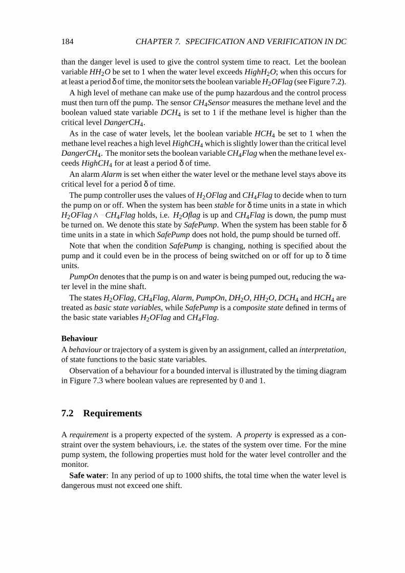
184 CHAPTER 7. SPECIFICATION AND VERIFICATION IN DC
than the danger level is used to give the control system time to react. Let the booleanvariable HH2O be set to 1 when the water level exceeds HighH2O; when this occurs forat least a period δ of time, the monitor sets the boolean variable H2OFlag (see Figure 7.2).
A high level of methane can make use of the pump hazardous and the control processmust then turn off the pump. The sensor CH4Sensor measures the methane level and theboolean valued state variable DCH4 is set to 1 if the methane level is higher than thecritical level DangerCH4.
As in the case of water levels, let the boolean variable HCH4 be set to 1 when themethane level reaches a high level HighCH4 which is slightly lower than the critical levelDangerCH4. The monitor sets the boolean variable CH4Flag when the methane level ex-ceeds HighCH4 for at least a period δ of time.
An alarm Alarm is set when either the water level or the methane level stays above itscritical level for a period δ of time.
The pump controller uses the values of H2OFlag and CH4Flag to decide when to turnthe pump on or off. When the system has been stable for δ time units in a state in whichH2OFlag^:CH4Flag holds, i.e. H2Oflag is up and CH4Flag is down, the pump mustbe turned on. We denote this state by SafePump. When the system has been stable for δtime units in a state in which SafePump does not hold, the pump should be turned off.
Note that when the condition SafePump is changing, nothing is specified about thepump and it could even be in the process of being switched on or off for up to δ timeunits.
PumpOn denotes that the pump is on and water is being pumped out, reducing the wa-ter level in the mine shaft.
The states H2OFlag, CH4Flag, Alarm, PumpOn, DH2O, HH2O, DCH4 and HCH4 aretreated as basic state variables, while SafePump is a composite state defined in terms ofthe basic state variables H2OFlag and CH4Flag.
BehaviourA behaviour or trajectory of a system is given by an assignment, called an interpretation,of state functions to the basic state variables.
Observation of a behaviour for a bounded interval is illustrated by the timing diagramin Figure 7.3 where boolean values are represented by 0 and 1.
7.2 Requirements
A requirement is a property expected of the system. A property is expressed as a con-straint over the system behaviours, i.e. the states of the system over time. For the minepump system, the following properties must hold for the water level controller and themonitor.
Safe water: In any period of up to 1000 shifts, the total time when the water level isdangerous must not exceed one shift.

7.2. REQUIREMENTS 185
DH2O
HH2O
H2OFlag
DCH4
HCH4
CH4Flag
SafePump
Alarm
PumpOn
10
Figure 7.3 Observation of a behaviour
Set flags: The flags H2OFlag and CH4Flag, respectively, must be set (or 1) when thewater or methane levels have been high for at least a period δ of time.
Reset flags: The flags H2OFlag and CH4Flag, respectively, must be cleared (or 0)when the water or methane levels have not been high for at least a period δ of time.
Safe waterFor an observation of the mine pump system behaviour in a bounded interval [b;e] oftime, the duration of DH2O is measured by the integral
R ebDH2O(t)dt, shown shaded in
the timing diagram in Figure 7.4.This duration is the total time for which the water level is dangerous. Thus the property
Safe water for an interval [b;e] is
(e�b)� 1000) R ebDH2O(t)dt � 1
To simplify reasoning, it is always desirable to avoid explicit reference to time in formu-las; thus, the use of t and the bounding points b and e together with universal quantifica-tion over the interval should be avoided. Let the symbol
RDH2O denote the duration of

186 CHAPTER 7. SPECIFICATION AND VERIFICATION IN DC
Time0
DH2O
1
b e
Figure 7.4 A duration of DH2O
DH2O. Let ` be the length of the interval. Then the property Safe water can be expressedwithout explicit mention of time as
`� 1000) RDH2O� 1
For a given behaviour of the mine pump and a given bounded interval (an observation),this formula is either true or false. A formula holds for a behaviour if it is true for anyprefix interval [0; t], t � 0, of the behaviour. Thus, the formula tells us that a behaviourof the mine pump is safe if for any prefix interval [0; t], t � 1000, the duration of DH2Oin that interval is not more than 1. But Safe water does not require the system to be safefor only the first 1000 shifts. So we need to express this property over any observationinterval [b;e], b� 0.
The modal operator 2 is used to denote that a formula holds for any subinterval of agiven observation. The property Safe states that for any subinterval of a given observa-tion, the duration of DH2O is at most 1.
Safe∆=2(` � 1000) RDH2O� 1)
The property holds for a behaviour when the constraint on DH2O holds for any subinter-val of any prefix interval, i.e. any bounded interval.
Set flagsThe requirement for the water level flag is that for an observation interval longer than δ,H2OFlag must be set to 1 when the water level has been high for at least a period δ oftime. So the constraint is that HH2O is true for a period δ of time, or more.
To express such properties, we need some notation to describe when a state P has beentrue in a non-point interval. The operator d�e lifts a state to a predicate (or a property).For state P, the property dPe holds for an interval [b;e] iff b < e and there are only finitemany t in this interval such that P(t) = 0. The formula dPe can be read as ‘P is true almosteverywhere in the non-point interval’. The value of P is ignored at possible points of dis-continuity and these will be a finite set for any finite observation. In particular, we avoiddiscussion of the values at end points, making it irrelevant whether we choose closed,open, or half-open intervals as the durations remain the same. Taking closed intervalsmay be intuitively a little bit clearer, because a point is an interval.

7.2. REQUIREMENTS 187
Timeb
F2
m e
F1
F1; F2
Figure 7.5 The chop operator
Exercise 7.2.1 Define dPe in terms ofR
P and `.
The property that HH2O holds for a period δ of time can now be written as
dHH2Oe^ (` = δ)
Similarly, if H2OFlag is 0 in an interval we have d:H2OFlage. These two formulas canbe combined to express the property Set flags using the binary modal operator chop. Theformula (F1 ; F2) is read as ‘F1 chop F2’: it holds in an interval [b;e] iff this interval canbe divided into an initial subinterval [b;m] in which F1 holds, and a final subinterval [m;e]in which F2 holds, b� m� e. This is illustrated by the timing diagram in Figure 7.5.
The property Set flags is defined using the chop operator as:
:((dHH2Oe^ `= δ); d:H2OFlage)
which states that it is not the case that the observation starts with DH2O holding for δunits of time followed by the water flag being off for a non-point subinterval.
The property should hold for all observations, so to complete the specification we have
2:(dHH2Oe^ `= δ) ; d:H2OFlage)
The formula can be rewritten using an abbreviation: for a formula F and a state P,
F t�! dPe
∆=2:(F ^ (`= t); d:Pe)
which is read as ‘F for time t leads to state P’; it is defined by stating that it is never thecase that F holds for time t and P does not then hold. A similar abbreviation reads ‘Ffor up to time t leads to state P’ and is defined below:
F �t�! dPe
∆=2:(F ^ (`� t) ; d:Pe)
Thus F can go to state P only after it has held for up to t time units.The setting of the flag to indicate a high water level is then specified as
SetWaterFlag∆= dHH2Oe
δ�! dH2OFlage
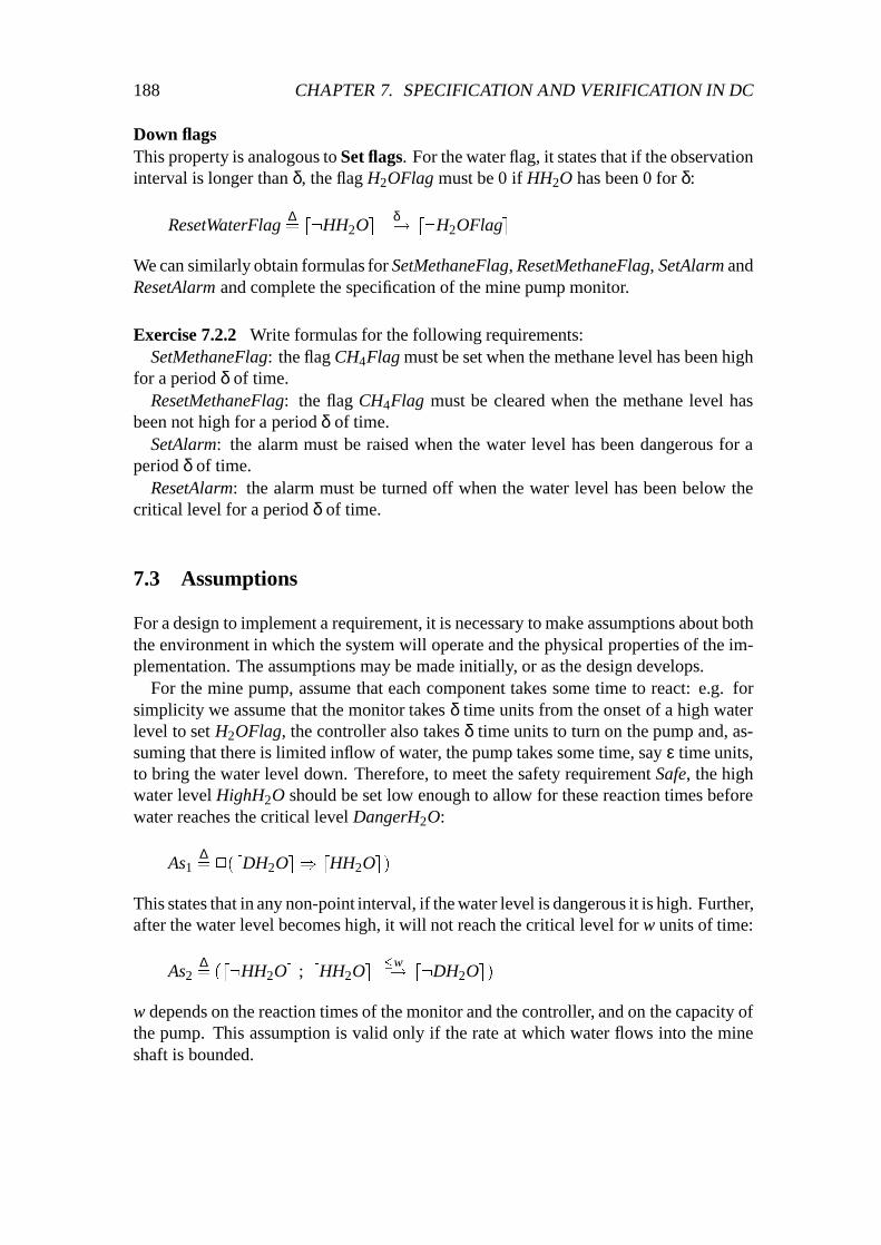
188 CHAPTER 7. SPECIFICATION AND VERIFICATION IN DC
Down flagsThis property is analogous to Set flags. For the water flag, it states that if the observationinterval is longer than δ, the flag H2OFlag must be 0 if HH2O has been 0 for δ:
ResetWaterFlag∆= d:HH2Oe
δ�! d:H2OFlage
We can similarly obtain formulas for SetMethaneFlag, ResetMethaneFlag, SetAlarm andResetAlarm and complete the specification of the mine pump monitor.
Exercise 7.2.2 Write formulas for the following requirements:SetMethaneFlag: the flag CH4Flag must be set when the methane level has been high
for a period δ of time.ResetMethaneFlag: the flag CH4Flag must be cleared when the methane level has
been not high for a period δ of time.SetAlarm: the alarm must be raised when the water level has been dangerous for a
period δ of time.ResetAlarm: the alarm must be turned off when the water level has been below the
critical level for a period δ of time.
7.3 Assumptions
For a design to implement a requirement, it is necessary to make assumptions about boththe environment in which the system will operate and the physical properties of the im-plementation. The assumptions may be made initially, or as the design develops.
For the mine pump, assume that each component takes some time to react: e.g. forsimplicity we assume that the monitor takes δ time units from the onset of a high waterlevel to set H2OFlag, the controller also takes δ time units to turn on the pump and, as-suming that there is limited inflow of water, the pump takes some time, say ε time units,to bring the water level down. Therefore, to meet the safety requirement Safe, the highwater level HighH2O should be set low enough to allow for these reaction times beforewater reaches the critical level DangerH2O:
As1∆=2(dDH2Oe ) dHH2Oe)
This states that in any non-point interval, if the water level is dangerous it is high. Further,after the water level becomes high, it will not reach the critical level for w units of time:
As2∆= (d:HH2Oe ; dHH2Oe
�w�! d:DH2Oe)
w depends on the reaction times of the monitor and the controller, and on the capacity ofthe pump. This assumption is valid only if the rate at which water flows into the mineshaft is bounded.

7.4. DESIGN 189
7.4 Design
Design involves making choices and taking decisions about how requirements are to bemet. For example, to meet the safety requirement Safe according to the assumptions As1and As2, it is necessary to bring a high water level down within w time units, i.e. beforeit reaches the critical level:
2(dHH2Oe ) `�w) or, equivalently, dHH2Oew�! d:HH2Oe
But this may not always be possible as a high methane level may make it unsafe for thecontroller to turn on the pump. The property Safe allows limited occurrences of danger-ous water levels provided they do not last too long or occur too often. Let
Failure∆= dHH2Oe^ ` > w
Since each occurrence of Failure takes at least time w and at most time 1, the followingtwo design decisions can be made:
� A Failure can only occur in an interval not longer than one time unit.� Any two occurrences of Failure must be separated by at least 1001 time units; in
other words, Failure occurs at most once in any interval that is not longer than1000.
The first decision can be easily formalized as
Des11∆=2(Failure ) `� 1)
The second decision says that if an observation interval can be divided into three adja-cent subintervals such that Failure holds in the first and last subintervals, and somewherein the middle subinterval Failure does not hold, then the observation interval must be atleast 1001 time units long.
This needs some notation to describe a property that holds somewhere in an interval,and the conventional modal operator 3 (read as ‘somewhere’) serves the need. For aformula F ,3F holds in an interval [b;e] iff there is a subinterval [b0;e0], b� b0 and e0 � e,such that F holds in [b0;e0]. This is illustrated by the following diagram:
Timeb eb0 e0
F
3F
The second design decision then becomes
Des12∆=2((Failure ; 3:Failure ; Failure)) `� 1001)

190 CHAPTER 7. SPECIFICATION AND VERIFICATION IN DC
At all times, if Failure is followed at some time by :Failure and then by Failure, thelength l of the observation interval must be at least 1001.
Let Des1∆= Des11^Des12. To verify that Des1 guarantees the safety requirement we
must prove the implication
Des1) Safe
But the implication does not hold without the assumptions As1 and As2 about the highwater level. So what we must prove is that the implication does hold under these as-sumptions:
As1^As2 ^Des1) Safe
Exercise 7.4.1 Give arguments for the validity of this implication in the context of themine pump.
In general, proving that the conjunction of assumptions and design decisions implies arequirement is called the verification of the correctness of the design with respect to therequirement. Such an implication has the form
A ^D) C
where A is the specification of the assumption, D is the specification of the design, andC is the specification of the requirement (i.e. commitment).
Note that A ^D ) C is equivalent to D ) (A ) C ). Thus, A ) C is sometimescalled the requirement, i.e. ‘the requirement is a commitment under the assumption’.
A design decision can be refined into lower level design decisions. For example, Des1can be refined into the following control plans:
1. The pump must be on when the water level has been high and the methane levelhas been low for δ time units:
StartPump∆= dSafePumpe δ�! dPumpOne
2. The pump must be off when the water level has been low or the methane level hasbeen high for δ time units:
StopPump∆= d:SafePumpe δ�! d:PumpOne
Let Des2∆= StartPump^ StopPump. To prove the correctness of this refined design
with respect to Des1, we need the following assumptions (these will be formalized inSection 7.6):
As3: assumption about the capacity of the pump.As4: assumption about the duration of a high methane level.Monitor: the full specification of the monitor as an assumption.As5: assumption about the choice of the constants w and δ.

7.5. THE BASIC DURATION CALCULUS (DC) 191
Then, the goal is to prove
As3^As4 ^As5^Monitor^Des2) Des1
This kind of refinement procedure can be repeated until an implementation of the systemis obtained. The correctness of the implementation is guaranteed by the transitivity of thelogical implication. For example, the two implications above guarantee the implication
As^Des2) Safe
where
As∆= As1 ^As2^As3 ^As4^As5 ^Monitor
The informal introduction in this section has provided a notation for the specification ofrequirements, assumptions and designs of real-time embedded systems. The mine pumpexample has been used to illustrate the steps in the formal development of such a system.But for formal verification of properties and the correctness of a design, we need a set ofaxioms and rules.
7.5 The basic duration calculus (DC)
The simplicity of temporal logic comes from the removal of explicit time. In IntervalTemporal Logic (ITL), the variables b and e, denoting the end points of an arbitrary ob-servation interval [b;e], are removed from expressions such as Safe and SetWaterFlag(Section 7.2). A variable v is interpreted as a function from intervals to values. A for-mula in ITL, such as v1 � v2, holds for an interval [b;e] under a given interpretation Iof v1 and v2; i.e. if I(v1)([b;e]) � I(v2)([b;e]) holds in the value domain. ITL uses themodal operator chop to define the usual modalities3 and 2.
DC develops on ITL by introducing integrals (i.e. durations) of states over intervalsas variables in the interval temporal logic. Thus, DC adopts primitives such as the chopoperator of ITL. We shall be concerned mainly about the axioms and rules dealing withintegrals of states. But we shall also consider some ITL axioms for the chop operator;although they will not be called axioms or theorems, they will be used to prove propertiesof durations.
7.5.1 Time
DC uses continuous time, Time, represented by the set of non-negative real numbers. t,t1, etc. are assumed to range over the real numbers. A time interval is a closed interval[b;e] of the real numbers, i.e. b;e 2 Time and b � e and [b;e] is the set of time pointsfrom b to e.

192 CHAPTER 7. SPECIFICATION AND VERIFICATION IN DC
7.5.2 States
A basic state is a state variable. An interpretation I assigns a basic state P to a functionI(P) from Time to the set f0;1g of boolean values. I(P)(t) = 1 means that state P is ‘on’at time t, and I(P)(t) = 0 that it is ‘off’ at time t, under the interpretation I. In the minepump example, DH2O, DCH4, HH2O and HCH4 are basic states. An observation of abehaviour of this system, such as the one illustrated by the diagram in Figure 7.3, givesan interpretation for these states over the observation interval.
States will be ranged over by P, Q, P1, Q1, etc., and will consist of expressions formedby the following rules:
� Each basic state P is a state.� If P and Q are states, then so are :P, (P^Q).
A composite state is interpreted as a function from Time to the set f0;1gwhich is definedby the interpretation for the basic states and the boolean operators. For example,
SafePump∆= HH2O^:HCH4
is a composite state. For an interpretation I and some t 2 Time,
I(SafePump)(t) = I(HH2O)(t)^:I(HCH4)(t)
The timing diagram in Figure 7.3 gives an illustration of an interpretation for SafePump.The conventional boolean operators_,) and, can be defined from: and^ in the usualway. Specifically, the constant state 0 and 1 can be defined as P^:P and:0 respectively.
7.5.3 Duration terms
The duration of a state P is denoted byR
P. Given an interpretation I of states, the dura-tion
RP is interpreted over time intervals and denotes the accumulated time when P is ‘on’
within the time interval. So, for an arbitrary interval [b;e], the interpretation I(R
P)([b;e])is defined as the integral of the function I(P) over the interval [b;e], i.e.
I(R
P)([b;e])∆=R e
bI(P)(t)dt
which is a real number. An interpretation for the durationR
DH2O was illustrated by thetiming diagram in Figure 7.4.
Let R denote the set of real numbers and be ranged over by logical variables x, y, z,with or without subscripts. The set of basic duration terms consists of variables and con-stants over the real numbers R, such as x and 5, and durations of states, such as
RP. A
duration term is either a basic duration term or an expression formed from duration termsusing the usual operators on real numbers, such as + (addition) and � (multiplication).For example,R
SafePump and 5� (RHCH4)� (R
SafePump)
are duration terms.

7.5. THE BASIC DURATION CALCULUS (DC) 193
7.5.4 Duration formulas
A basic duration formula is an expression formed from duration terms using the usualrelational operators on real numbers, such as = (equality) and < (inequality), with theirstandard meanings. The set of duration formulas, ranged over by F , G, etc., consists ofexpressions formed by the following rules:
� Each basic duration formula is a duration formula.� If F and G are duration formulas, so are :F , F ^G.� If F is a duration formula and x is a logical variable over the real numbers, then9x:F is a duration formula.
� If F and G are duration formulas, so is (F ; G).
As before, the first-order logic operators_,) and, can be defined in terms of the givenoperators : and ^; the universal quantifier 8 can be defined in terms of the given quan-tifier 9 and the operator : in the usual way.
In these definitions, we use the conventional rules of precedence for each first-orderoperator; e.g. : has the highest precedence and the precedence of conjunction^ is higherthan that of disjunction _. In addition, the precedence of the chop operator is higher thanthat of implication and lower than that of disjunction.
A duration formula F is satisfied by an interpretation I over an interval [b;e] when itevaluates to true. This satisfaction relation is written as
I; [b;e] j= F
For example, if I1 assigns HH2O to 1 over [0;2], and assigns HCH4 to 0 over [0;1) andto 1 over (1;2], we have
I1; [0;2]j=(2� R SafePump) =R
HH2O I1; [0;1] j=R
SafePump = 1I1; [1;2]j=
RSafePump = 0 I1; [0:5;1]j=
RHH2O =
RSafePump
Exercise 7.5.1 For the interpretation I1 for HH2O and HCH4, find two subintervals of[0;2] such that 3� R SafePump <
RHH2O holds in one subinterval but not in the other.
The ‘chopped’ formula (F ; G) is true for an interpretation I within interval [b;e] ifthere exists m such that b � m � e and F and G are true for I with [b;m] and [m;e] re-spectively; i.e.
I; [b;m] j= F and I; [m;e] j= G
The timing diagram in Figure 7.5 illustrates the semantics of the chop operator. As anexample, considering again interpretation I1 for HH2O and HCH4 over [0;2], we have
I1; [0;2] j= (R
SafePump = 1) ; (R
SafePump = 0)

194 CHAPTER 7. SPECIFICATION AND VERIFICATION IN DC
Exercise 7.5.2 Under the interpretation I1, find a subinterval of [0;2] for which
true ; (R
SafePump =R
1); true
holds but the following formula does not hold:
:(true ; :(R SafePump =R
1); true)
Give an informal meaning to these two formulas.
A duration formula is valid if it is true for any interpretation over any bounded timeinterval. For example,
RP+
R:P =R
1
is valid. More obviously,R
P� R 1 is valid.
7.5.5 Axioms and rules
We are now in a position to define the axioms and rules with which to calculate the du-rations of states.
We begin by listing some simple theorems of analysis which are sufficiently useful tobe taken as axioms in the calculus.
Axiom 7.1R
0 = 0.
Axiom 7.2 For an arbitrary state P,R
P� 0.
Axiom 7.3 For arbitrary states P and Q,R
P+R
Q =R(P_Q)+
R(P^Q).
Using these axioms, we can readily prove properties such as the following theorem.
Theorem 7.1 For an arbitrary state P
(a)R
P+R:P =
R1 (b)
RP� R 1
Proof: (a):R
P+R:P =
R(P_:P)+
R(P^:P) Axiom 3
=R
1+R
0 boolean operations=
R1 Axiom 1
Proof of (b) follows from (a) and Axiom 2.2
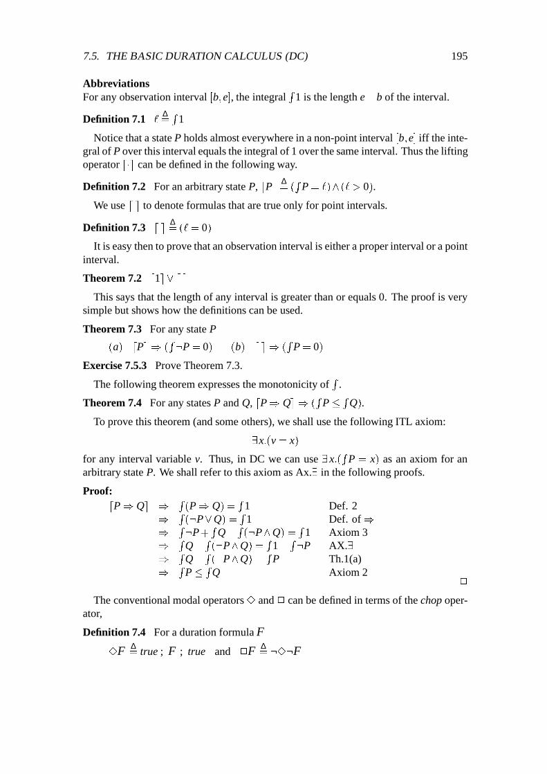
7.5. THE BASIC DURATION CALCULUS (DC) 195
AbbreviationsFor any observation interval [b;e], the integral
R1 is the length e�b of the interval.
Definition 7.1 `∆=R
1
Notice that a state P holds almost everywhere in a non-point interval [b;e] iff the inte-gral of P over this interval equals the integral of 1 over the same interval. Thus the liftingoperator d�e can be defined in the following way.
Definition 7.2 For an arbitrary state P, dPe ∆= (R
P = `)^ (` > 0).
We use d e to denote formulas that are true only for point intervals.
Definition 7.3 d e ∆= (`= 0)
It is easy then to prove that an observation interval is either a proper interval or a pointinterval.
Theorem 7.2 d1e_d eThis says that the length of any interval is greater than or equals 0. The proof is very
simple but shows how the definitions can be used.
Theorem 7.3 For any state P
(a) dPe ) (R:P = 0) (b) d e ) (
RP = 0)
Exercise 7.5.3 Prove Theorem 7.3.
The following theorem expresses the monotonicity ofR
.
Theorem 7.4 For any states P and Q, dP) Qe ) (R
P� RQ).
To prove this theorem (and some others), we shall use the following ITL axiom:
9x:(v = x)
for any interval variable v. Thus, in DC we can use 9x:(R
P = x) as an axiom for anarbitrary state P. We shall refer to this axiom as Ax.9 in the following proofs.
Proof:dP) Qe ) R
(P) Q) =R
1 Def. 2) R
(:P_Q) =R
1 Def. of)) R:P+
RQ� R (:P^Q) =
R1 Axiom 3
) RQ� R (:P^Q) =
R1� R:P AX.9
) RQ� R (:P^Q) =
RP Th.1(a)
) RP� RQ Axiom 2
2
The conventional modal operators 3 and 2 can be defined in terms of the chop oper-ator,
Definition 7.4 For a duration formula F
3F ∆= true ; F ; true and 2F ∆
= :3:F

196 CHAPTER 7. SPECIFICATION AND VERIFICATION IN DC
Properties of the chop operatorWe now present some basic properties of the ITL chop operator which we shall use asaxioms.
The first property, referred to as the chop-unit, is that the chop operator has d e as unit.Formally, for an arbitrary duration formula F :
(a) d e; F , F (b) F ; d e , F
The chop operator has false as zero. That is, for an arbitrary duration formula F :
(a) false; F , false (b) F ; false, false
We shall call this property chop-zero. It means that no interval can be split into two subin-tervals such that false holds for the first or the last subinterval, since false does not holdfor any interval.
The chop operator is associative, denoted as chop-associative; i.e. for any durationformulas F1, F2 and F3
(F1; F2); F3 , F1; (F2; F3)
and both sides of this formula can be written as F1; F2; F3.The chop operator is distributive through disjunction; i.e. for any duration formulas
F1, F2 and F3
F1; F2_F3 , (F1; F2)_ (F1; F3)
This property is called chop-distributive.
Exercise 7.5.4 Find a counter-example to show that the chop operator does not dis-tribute through conjunction.
The chop operator is monotonic, referred to as chop-monotonic; i.e. for any durationformulas F1, F2 and F3
2(F1 ) F2))2((F1; F3 ) F2; F3)^ (F3; F1 ) F3; F2))
The basic axiom relating the chop operator and the integral operator states that the du-ration of a state in an interval is the sum of its durations in each partition of the intervalinto subintervals.
Axiom 7.4 Let P be a state and r, s be non-negative real-numbers:
(R
P = r+ s), (R
P = r); (R
P = s)
With these axioms, we can prove properties such as the following theorem.
Theorem 7.5 For a state P and non-negative real numbers r, s, t and u
(r�R
P� s); (t �R
P � u)) (r+ t �R
P � s+u)

7.5. THE BASIC DURATION CALCULUS (DC) 197
Proof:
r� RP ; t� RP , 9x:9y:((R
P = x;R
P = y)^ (r � x^ t � y)) Ax.9, 9x:9y:((
RP = x+ y)^ (r � x^ t� y)) Ax.4
) 9x:9y:((R
P = x+ y)^ (r+ t � x+ y)), r+ t� RP Ax.9
Proof ofR
P� s ;R
P� u is similar (and is left as an exercise).2
The next theorem is about the arbitrary divisibility of intervals, i.e. the density of time.
Theorem 7.6 For a state P
dPe; dPe , dPe
Exercise 7.5.5 Prove Theorem 7.6.
It is useful to have an induction rule which extends a hypothesis over adjacent subin-tervals. Such a rule relies on the finite variability of states and the finiteness of intervals,so that any interval can be split into a finite alternation of state P and state :P.
Induction rule: For a formula variable X occurring in the duration formula R(X), andstate P:
1. If R(d e) holds, and R(X _ (X ; dPe) _ (X ; d:Pe)) is provable from R(X), thenR(true) holds.
2. If R(d e) holds, and R(X _ (dPe ; X) _ (d:Pe ; X)) is provable from R(X), thenR(true) holds.
The following theorem illustrates the use of the induction rules.
Theorem 7.7 For state P:
1. (true ; dPe)_ (true ; d:Pe)_d e2. (dPe ; true)_ (d:Pe ; true)_d e
Proof:(1) As the induction hypothesis, let
R(X)∆= X) ((true ; dPe)_ (true ; d:Pe)_d e)
Then for X = d e
R(d e) ∆= d e ) ((true ; dPe)_ (true ; d:Pe)_d e)
must hold. Now R(X_ (X ; dPe)_ (X ; d:Pe)) is
X_ (X ; dPe)_ (X ; d:Pe)) ((true ; dPe)_ (true ; d:Pe)_d e)

198 CHAPTER 7. SPECIFICATION AND VERIFICATION IN DC
Assuming that R(X) holds, the following formulas hold since X ) true holds and thechop operator is monotonic:
X) ((true ; dPe)_ (true ; d:Pe)_d e)
X ; dPe ) true ; dPe and X ; d:Pe ) true ; d:Pe
So it must be that R(X_ (X ; dPe)_ (X ; d:Pe)). Hence, by the induction rule, we haveR(true) holds which, by definition, is
true) ((true ; dPe)_ (true ; d:Pe)_d e)
This is obviously equivalent to (1).(2) can be proved symmetrically using the second induction rule.
2
The four axioms and the induction rules can be shown to constitute a sound formal proofsystem of durations which is relatively complete with respect to the interval temporallogic.
7.6 The mine pump
We are now ready to formally verify the correctness of the design of the mine pump sys-tem. We first summarize the specifications given in Sections 7.1–7.4.
Specification of the safety requirementFor the mine pump system, in any observation interval that is not longer than 1000 timeunits the accumulated time when the water level is dangerous is not more than one timeunit. This safety requirement is specified as
Safe∆=2(` � 1000) RDH2O� 1)
Specification of the monitorThe monitor is required to behave in the following way:
1. The water flag H2OFlag must be set when the water level has been high for δ timeunits and cleared when it has not been high for that time; likewise for the methaneflag CH4Flag.
2. The alarm must be set when either the water level or the methane level has beendangerous for δ time units and cleared when they have both been below the dangerlevel for δ time units.

7.6. THE MINE PUMP 199
The monitor is specified by the following formulas:
SetWaterFlag∆= dHH2Oe
δ�! dH2OFlage
ResetWaterFlag∆= d:HH2Oe
δ�! d:H2OFlage
SetMethaneFlag∆= dHCH4e
δ�! dCH4Flage
ResetMethaneFlag∆= d:HCH4e
δ�! d:CH4Flage
SetAlarm∆= dDH2Oe
δ�! dAlarme
^ dDCH4eδ�! dAlarme
ResetAlarm∆= d:DH2O^:DCH4e
δ�! d:Alarme
Monitor∆= SetWaterFlag^ResetWaterFlag
^ SetMethaneFlag^ResetMethaneFlag^ SetAlarm^ResetAlarm
Specification of assumptionsThe high water level is lower than the dangerous water level; in other words, if the waterlevel is dangerous, it must also be high:
As1∆=2(dDH2Oe ) dHH2Oe)
The high water level is chosen such that, after it has been reached, the water will not reachthe critical level within w units of time:
As2∆= (d:HH2Oe ; dHH2Oe)
�w�! d:DH2Oe
The capacity of the pump is sufficient to bring the water level down to a level lower thanthe high level in ε units of time:
As3∆= dPumpOne
ε�! d:HH2Oe
If the methane level is stable at a low level for long enough, and the methane level is highfor a sufficiently short time, it should always be possible to turn on the pump and reducethe water level before it reaches the dangerous level. This stability and boundedness canbe specified, respectively, as
StableCH4∆= (dHCH4e ; d:HCH4e ; dHCH4e)) `� ξ
BoundCH4∆= dHCH4e ) `� w�2ξ
Recall that Safe allows limited occurrences of dangerous water levels. This means that itallows limited failure in reducing the high water levels. So we do not have to assume thatStableCH4 and BoundCH4 always hold, i.e. bad methane levels are sometimes allowed.Let
BadCH4∆= :(StableCH4^BoundCH4)

200 CHAPTER 7. SPECIFICATION AND VERIFICATION IN DC
To constrain bad methane levels, we assume that they will occur only in an interval notlonger than one time unit; any two occurrences of bad methane levels must be separatedby at least 1001 time units. The conjunction of these two constraints is specified as
As4∆= 2(BadCH4 ) `� 1)
^ 2((BadCH4 ; 3:BadCH4 ; BadCH4)) `� 1001)
Finally, the constants must be chosen in the following way:
As5∆= (ξ � 2δ+ ε)^ (w� 2ξ)
Specification of the designRefinements to the safety requirements were made in two steps in Section 7.4: the firststep was to make the design decision that in any interval not longer than 1000 time units,the high water level must almost always be reduced within w time units, i.e. before itreaches the dangerous level:
Des1∆= 2(Failure ) `� 1)
^ 2((Failure ; 3:Failure ; Failure)) `� 1001)
where Failure∆= dHH2Oe^ ` > w.
The second step was to decide the control strategies of the pump:
Des2∆= StartPump^StopPump
where
StartPump∆= dSafePumpe
δ�! dPumpOne
StopPump∆= d:SafePumpe
δ�! d:PumpOne
Recall that SafePump∆= HH2O^:HCH4.
Proving correctnessWe shall state correctness results as theorems and then provide proofs.
Theorem 7.8 As1 ^As2^Des1 ) Safe
This theorem is derived from the following lemma:
Lemma 7.1
1: (`� 1000)^Des1 ) 2Failure^ ` � 1_ Failure^ `� 1 ; 2:Failure_ 2:Failure ; Failure^ `� 1 ; 2:Failure
2: As1^As2 ^2:Failure^ (d:HH2Oe ; true))R
DH2O = 0

7.6. THE MINE PUMP 201
Proof: We prove case (2) of the lemma. Recall that
:Failure = dHH2Oe ) `� w
Therefore, we have to prove that
As1^As2 ^2(dHH2Oe ) `� w)^ (d:HH2Oe ; true)) RDH2O = 0
Let A ∆= As1^As2 ^2(dHH2Oe ) `� w). Use the second induction rule with R(X)
defined as
R(X)∆= A ^ (d:HH2Oe ; X)) (
RDH2O = 0)
^ A ^ (d:HH2Oe ; dHH2Oe ; X)) (R
DH2O = 0)
R(d e) holds since A ^d:HH2Oe ) d:DH2Oe because of As1. And, by As2,
A ^ (d:HH2Oe ; dHH2Oe^ `� w)) d:DH2Oe
Using the chop-distributive property and Theorem 7.6:
R(X_ (dHH2Oe ; X)_ (d:HH2Oe ; X)), A ^ ((d:HH2Oe ; X)_ (d:HH2Oe ; dHH2Oe ; X))) (
RDH2O = 0)
^ A ^ (d:HH2Oe ; dHH2Oe ; d:HH2Oe)) (R
DH2O = 0)
We next prove that this formula holds assuming that R(X) holds. The first conjunct comesdirectly from R(X). For the second conjunct:
A ^ (d:HH2Oe ; dHH2Oe ; d:HH2Oe ; X)) d:HH2Oe ; dHH2Oe^ (`� w) ; d:HH2Oe ; X (2:Failure)) d:DH2Oe ; d:HH2Oe ; X (As1 ^As2)) R
DH2O = 0 ;R
DH2O = 0 (R(X))) R
DH2O = 0 (Axiom4)
Hence case 2 of the lemma is implied by R(true).
2
Exercise 7.6.1 Complete the proof of the lemma, and then prove Theorem 7.8.
Theorem 7.9 As3 ^As4^As5 ^Monitor^Des2) Des1
This theorem can be proved using the following lemma.
Lemma 7.2 As3^As4 ^2:BadCH4^Monitor)2:Failure
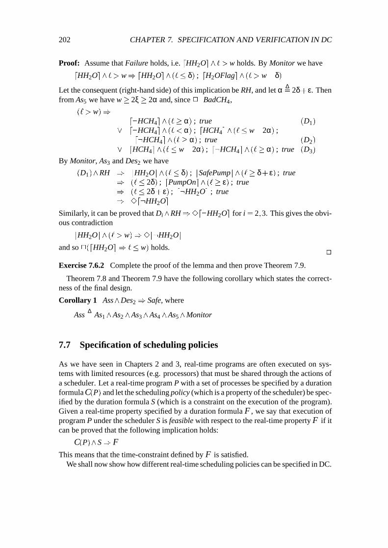
202 CHAPTER 7. SPECIFICATION AND VERIFICATION IN DC
Proof: Assume that Failure holds, i.e. dHH2Oe^ ` > w holds. By Monitor we have
dHH2Oe^ ` > w) dHH2Oe^ (`� δ) ; dH2OFlage^ (` > w�δ)
Let the consequent (right-hand side) of this implication be RH, and let α ∆= 2δ+ε. Then
from As5 we have w � 2ξ � 2α and, since 2:BadCH4,
(` > w))d:HCH4e^ (`� α) ; true (D1)
_ d:HCH4e^ (` < α) ; dHCH4e^ (`� w�2α) ;d:HCH4e^ (`� α) ; true (D2)
_ dHCH4e^ (`� w�2α) ; d:HCH4e^ (`� α) ; true (D3)
By Monitor, As3 and Des2 we have
(D1)^RH ) dHH2Oe^ (`� δ) ; dSafePumpe^ (`� δ+ ε) ; true) (`� 2δ) ; dPumpOne^ (`� ε) ; true) (`� 2δ+ ε) ; d:HH2Oe ; true) 3d:HH2Oe
Similarly, it can be proved that Di^RH )3d:HH2Oe for i = 2;3. This gives the obvi-ous contradiction
dHH2Oe^ (` > w))3d:HH2Oe
and so 2(dHH2Oe ) `� w) holds.2
Exercise 7.6.2 Complete the proof of the lemma and then prove Theorem 7.9.
Theorem 7.8 and Theorem 7.9 have the following corollary which states the correct-ness of the final design.
Corollary 1 Ass^Des2 ) Safe, where
Ass∆= As1^As2 ^As3^As4 ^As5^Monitor
7.7 Specification of scheduling policies
As we have seen in Chapters 2 and 3, real-time programs are often executed on sys-tems with limited resources (e.g. processors) that must be shared through the actions ofa scheduler. Let a real-time program P with a set of processes be specified by a durationformula C (P) and let the scheduling policy (which is a property of the scheduler) be spec-ified by the duration formula S (which is a constraint on the execution of the program).Given a real-time property specified by a duration formula F , we say that execution ofprogram P under the scheduler S is feasible with respect to the real-time property F if itcan be proved that the following implication holds:
C (P)^S ) FThis means that the time-constraint defined by F is satisfied.
We shall now show how different real-time scheduling policies can be specified in DC.

7.6. THE MINE PUMP 203
Processes and processorsFor simplicity, assume that a set of processes is allocated statically to n > 0 processors.Such an allocation defines a partition of the processes into n classes fPS1; : : :;PSng. LetPS = fp1; : : :;pmg be an arbitrary class of this partition containing m > 0 processes shar-ing one processor. For each process p 2 PS:
� p:rdy : is 1 when process p is ready to run on a processor, otherwise it is 0.� p:run: is 1 when process p is running on a processor, otherwise it is 0.
We assume that when a process is running it is ready, i.e. p:run) p:rdy is always 1. Thisassumption is illustrated in the following timing diagram.
Time
p.rdy
p.run
SpecificationThere is a physical no conflict requirement that at most one process is running on a pro-cessor at any time:
2^k 6=j
(dpj:rune ) d:pk:rune)
or, equivalently,
2^k 6=j
(R(Pj:run^pk:run) = 0)
Assume that if a process is ready, there must be a running process:
2(d_
j
pj:rdye ) d_
j
pj:rune)
This means that the scheduler has no overhead, i.e. takes no time to initiate execution ofa process on a processor.
A scheduler is said to make progress if
2((∑i
Rpi:rdy > δ)) (∑
i
Rpi:run > δ0))
where δ and δ0 are constants such that 0 � δ0 � δ. This says that at all times if the sumof the ready time of the processes is greater than δ, the sum of their running times mustbe greater than δ0. Thus, progress will always be made in the execution of the processesin terms.
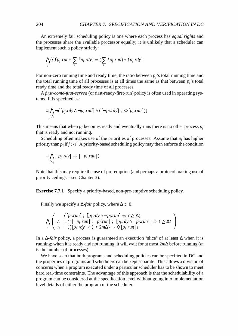
204 CHAPTER 7. SPECIFICATION AND VERIFICATION IN DC
An extremely fair scheduling policy is one where each process has equal rights andthe processes share the available processor equally; it is unlikely that a scheduler canimplement such a policy strictly:
^
j
((R
pj:run�∑i
Rpi:rdy) = (∑
i
Rpj:run)�
Rpj:rdy)
For non-zero running time and ready time, the ratio between pj’s total running time andthe total running time of all processes is at all times the same as that between pj’s totalready time and the total ready time of all processes.
A first-come-first-served (or first-ready-first-run) policy is often used in operating sys-tems. It is specified as:
2^
j6=i
:(dpj:rdy^:pi:rune^ (d:pi:rdye ; 3dpi:rune))
This means that when pi becomes ready and eventually runs there is no other process pj
that is ready and not running.Scheduling often makes use of the priorities of processes. Assume that pj has higher
priority than pi if j> i. A priority-based scheduling policy may then enforce the condition
2^
i<j
(dpj:rdye ) d:pi:rune)
Note that this may require the use of pre-emption (and perhaps a protocol making use ofpriority ceilings – see Chapter 3).
Exercise 7.7.1 Specify a priority-based, non-pre-emptive scheduling policy.
Finally we specify a ∆-fair policy, where ∆ > 0:
^
i
0@
(dpi:rune ; dpi:rdy^:pi:rune ) `� ∆)^ 2((d:pi:rune ; dpi:rune ; dpi:rdy^:pi:rune)) `� ∆)^ 2((dpi:rdye^ `� 2m∆))3dpi:rune)
1A
In a ∆-fair policy, a process is guaranteed an execution ‘slice’ of at least ∆ when it isrunning; when it is ready and not running, it will wait for at most 2m∆ before running (mis the number of processes).
We have seen that both programs and scheduling policies can be specified in DC andthe properties of programs and schedulers can be kept separate. This allows a division ofconcerns when a program executed under a particular scheduler has to be shown to meethard real-time constraints. The advantage of this approach is that the schedulability of aprogram can be considered at the specification level without going into implementationlevel details of either the program or the scheduler.

7.8. PROBABILISTIC DURATION CALCULUS (PDC) 205
7.8 Probabilistic duration calculus (PDC)
The requirements for an embedded, real-time system include functional and safety prop-erties. For the mine pump, we proved that the design decisions Des1 and Des2 guaranteethe requirement Safe. But, in practice, we cannot expect an actual implementation to sat-isfy this requirement at all times. For example, any physical component such as a sensor,the monitor, or the pump may fail to react in time.
Within any given period, an actual implementation can only satisfy the design deci-sions with a certain probability. How then can we model the physical limitations of animplementation? How can we define and reason about the probability of satisfaction ofa duration formula? The solution here, as in other fields, is to analyze the probability offailure using probability theory.
Assume that we consider not only the correct system behaviours BC = fb1; : : :g butalso some incorrect, but plausible, failure behaviours BF = ff1; : : :g. The model for animplementation is then B =BC[BF and probabilities can be assigned to subsets of B. Inthis section, we consider how to calculate the probability of a subset specified by someduration formula D for some finite initial segment [0; t] of the behaviours. This proba-bilistic extension of DC makes it possible for designers of real-time systems to reasonabout and calculate the probability that safety and functionality requirements are satis-fied in practical implementations.
In the probabilistic duration calculus (PDC), it is assumed that requirements are ex-pressed as formulas in DC, and that imperfect (i.e. failure-prone) designs can be modelledusing probabilistic automata with fixed transition probabilities. Then discrete Markovchains can provide the basis for PDC.
The calculus provides a notation and a set of rules for determining the probability thata given duration formula D holds for a given probabilistic automaton over a specifiedtime interval [0; t]. This probability, called the satisfaction probability µ(D)[t], is definedas the sum of the probabilities of all behaviours of the automaton which satisfy D overthe time interval.
DC uses continuous time represented by non-negative real-numbers. In order to havea simple, well-understood probabilistic model (see Section 7.8.1), discrete time is usedin PDC; thus, Time is the set of all non-negative integers. For this discrete time domain,axiom 4 of Section 7.5 must be modified.
For a state P and non-negative integers r, s, t and u:
(r�R
P� s) ; (t �R
P � u)) (r+ t �R
P� s+u)
Accordingly, Theorem 7.6 is also modified; for any state P:
`� 2) (dPe , dPe ; dPe)
No other axioms or rules of DC need to be changed.In this section, we define the reliability of two simplified versions of the mine pump.
In both cases, we ignore the methane levels. The satisfaction probability µ(D)[t] is thendefined as the sum of probabilities of all behaviours that satisfy D in the time interval
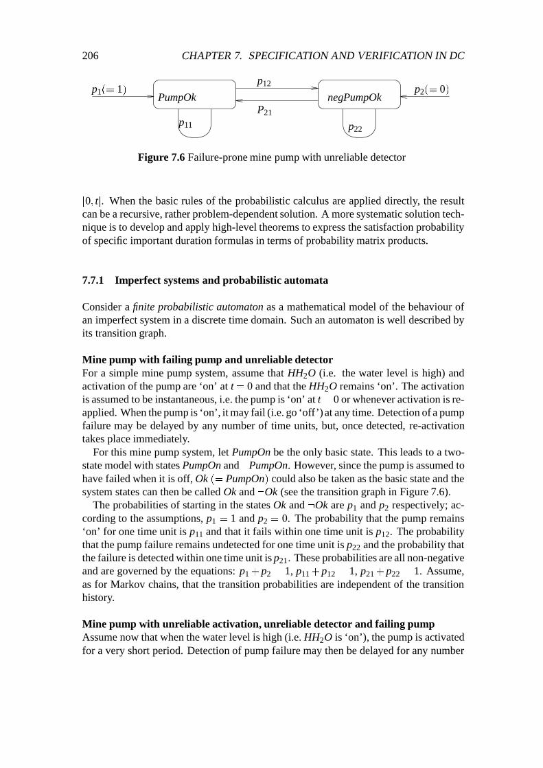
206 CHAPTER 7. SPECIFICATION AND VERIFICATION IN DC
p22
negPumpOkp2(= 0)
p11
PumpOkp1(= 1)
p12
P21
Figure 7.6 Failure-prone mine pump with unreliable detector
[0; t]. When the basic rules of the probabilistic calculus are applied directly, the resultcan be a recursive, rather problem-dependent solution. A more systematic solution tech-nique is to develop and apply high-level theorems to express the satisfaction probabilityof specific important duration formulas in terms of probability matrix products.
7.7.1 Imperfect systems and probabilistic automata
Consider a finite probabilistic automaton as a mathematical model of the behaviour ofan imperfect system in a discrete time domain. Such an automaton is well described byits transition graph.
Mine pump with failing pump and unreliable detectorFor a simple mine pump system, assume that HH2O (i.e. the water level is high) andactivation of the pump are ‘on’ at t = 0 and that the HH2O remains ‘on’. The activationis assumed to be instantaneous, i.e. the pump is ‘on’ at t = 0 or whenever activation is re-applied. When the pump is ‘on’, it may fail (i.e. go ‘off’) at any time. Detection of a pumpfailure may be delayed by any number of time units, but, once detected, re-activationtakes place immediately.
For this mine pump system, let PumpOn be the only basic state. This leads to a two-state model with states PumpOn and :PumpOn. However, since the pump is assumed tohave failed when it is off, Ok (= PumpOn) could also be taken as the basic state and thesystem states can then be called Ok and :Ok (see the transition graph in Figure 7.6).
The probabilities of starting in the states Ok and :Ok are p1 and p2 respectively; ac-cording to the assumptions, p1 = 1 and p2 = 0. The probability that the pump remains‘on’ for one time unit is p11 and that it fails within one time unit is p12. The probabilitythat the pump failure remains undetected for one time unit is p22 and the probability thatthe failure is detected within one time unit is p21. These probabilities are all non-negativeand are governed by the equations: p1 +p2 = 1, p11+p12 = 1, p21+p22 = 1. Assume,as for Markov chains, that the transition probabilities are independent of the transitionhistory.
Mine pump with unreliable activation, unreliable detector and failing pumpAssume now that when the water level is high (i.e. HH2O is ‘on’), the pump is activatedfor a very short period. Detection of pump failure may then be delayed for any number

7.7. PROBABILISTIC DURATION CALCULUS (PDC) 207
of time units. When HH2O is ‘on’, the pump may be off on account of activation failureor pump failure. Assume that when HH2O is ‘off’, the pump is also off.
The transition graph for this system is shown in Figure 7.7 There are two basic states:HH2O (water level is high) and PumpOn (pump is on).
At any time, the system is in one of the following mutually exclusive states:
V = f:HH2O^:PumpOn ; HH2O^PumpOn ; HH2O^:PumpOng
i.e. we assume that
:HH2O^PumpOn = 0
and
:HH2O^:PumpOn_HH2O^PumpOn_HH2O^:PumpOn = 1
The system probabilities are defined below:
� The system starts in the idle state :HH2O^:PumpOn: p1 = 1, p2 = p3 = 0.� It remains idle with probability p11 for one time unit.� HH2O becomes ‘on’ (water level becomes high) in one time unit with probability(p12+p13) and the pump is activated. p12 is the probability that activation succeedsand p13 that it fails.
� HH2O becomes ‘off’ within one time unit with probability p21.� The pump remains on for one time unit with probability p22.� The pump fails within one time unit with probability p23.� Pump failure is detected in one time unit with probability p32.� Pump failure remains undetected for one time unit with probability p33.
Notice that p31 is assumed to be zero. This means that when the pump fails, the waterlevel cannot be reduced.
These probabilities are non-negative and are related by the following equations: p1 +
p2 + p3 = 1 and pi1 + pi2 + pi3 = 1, (i = 1;2;3). Ok is now a composite state: Ok∆=
:HH2O_PumpOn.
Probabilistic automatonWe end with a general definition of a probabilistic automaton (PA). First define a mintermof a set A of basic states as a conjunction of the states in A which contains every state inA or its negation, but not both.
Definition 7.5 A PA is a tuple G = (A;V;τ0;τ) where the following hold:
� A is a finite, non-empty set of basic states.� V = fv1; : : :;vmg is a non-empty set of states; each vi in V is a minterm of A and
V is ranged over by v, v0, vi, etc.

208 CHAPTER 7. SPECIFICATION AND VERIFICATION IN DC
HH20 PumpOn
p22
p2(=0)
p11
p1(=1)HH2O PumpOn
p31(=0)
p13
p33
p3(=0)HH2O PumpOn
p21p12 p23 p32
Figure 7.7 Mine pump with unreliable activation, unreliable detector and failing pump
� τ0 : V ! [0;1] is called the initial probability mass function and it satisfies
∑v2V
τ0(v) = 1
where τ0(v) is the probability that the system starts in state v.� τ : V�V ! [0;1] is called the single-step probability transition function: for every
v 2 V it satisfies
∑v02V
τ(v;v0) = 1
For example, in Figure 7.6, A= fOkg, V = f:Ok;Okg. The initial probability mass func-tion is τ0(Ok) = p1 = 1, τ0(:Ok) = p2 = 0, and the transition probability function is
τ(Ok;Ok) = p11 τ(Ok;:Ok) = p12τ(:Ok;Ok) = p21 τ(:Ok;:Ok) = p22
7.8.2 Satisfaction probability
For a given automaton G = (A;V;τ0;τ), we now define behaviour, satisfaction and sat-isfaction probability.

7.7. PROBABILISTIC DURATION CALCULUS (PDC) 209
BehaviourGiven a non-negative integer t, the sequence of states in V,
σ[t] : v1; : : :;vt
defines a possible behaviour of G for its first t units of operation. Thus the system per-forms t�1 state transitions such that it is in state vi at time i�1, (i = 1; : : :; t).
For a specified sequence of states, v1; : : :;vt the probability that the system enters statev1 at time 0 is τ0(v1), and, given that it is in state vi at time i�1, the probability that it isin state vi+1 at time i is τ(vi;vi+1). Therefore, τ0 and τ together determine the probabilityof the behaviour σ[t] for the first t time units.
For example, σ[1] =:Ok is a behaviour of length 1 of the PA of Figure 7.6. Accordingto this, the system starts with :Ok. But τ0(:Ok) = p2 = 0, so the system cannot startwith :Ok. So the probability of σ[1] is zero. Let µ(σ[1]) denote the probability of σ[1]
with respect to the given PA; then µ(σ[1]) = 0.
σ[5] : Ok;Ok;:Ok;:Ok;Ok
is another behaviour of this PA, with length 5. For this behaviour,
µ(σ[5]) = p1 �p11 �p12 �p22 �p21
In general, if σ[t] = v1; : : :;vt,
µ(σ[t])∆= τ0(v1)�
t�1
∏i=1
τ(vi;vi+1)
where µ(σ[t]) = 1 when t = 0 and µ(σ[t]) = τ0(v1) when t = 1. Let Vt be the set of allstate sequences of V with length t. Then, Vt defines all the possible behaviours of G withlength t. From the definitions of τ0 and τ, it is easy to prove the following theorems.
Theorem 7.10 For any non-negative integer t and any behaviour σ[t] 2 Vt of length t,
0� µ(σ[t])� 1
Theorem 7.11 For any non-negative integer t, ∑σ[t]2Vt µ(σ[t]) = 1.
Thus, for every non-negative integer t there is a probability space hVt;µi with Vt, theset of behaviours of length t, as the set of samples.

210 CHAPTER 7. SPECIFICATION AND VERIFICATION IN DC
SatisfactionA behaviour σ[t] of G determines the presence and absence of the basic states in V at eachof the first t time units, and thus defines an interpretation Iσ[t] of duration formulas withA as the basic states for the first t time units. This interpretation is defined by:
Iσ[t](P)(j)∆=
�1 if σ(j)) P0 if σ(j)):P
where 0� j� t.Recalling Section 7.2, the satisfaction of a duration formula D (with A as basic states)
can be defined by a behaviour σ[t] of G.D is satisfied by σ[t], denoted by σ[t] j= D, if and only if there is an interpretation I
which is an extension of Iσ[t] over [0; t], such that I; [0; t] j= D. An interpretation I2 overTime is an extension of I1 over the interval [t1; t2] if for every basic state P and any timepoint t 2 [t1; t2], I1(P) = I2(P).
For the PA of Figure 7.6, let σ[5] ∆= Ok, Ok, :Ok, :Ok, Ok. Then,
σ[5] j= `= 5; σ[5] j= ROk = 3; σ[5] j=2(d:Oke ) `� 2)
σ[5] 6j= `� 3; σ[5] 6j=2(d:Oke ) `� 1)
where 6j= stands for ‘not satisfied’.
Satisfaction probabilityThe probability that a PA satisfies a duration formula over the time interval [0; t] is thesum over all behaviours of the probability that a behaviour satisfies the formula over thattime interval. Let D be a duration formula, and let Vt(D) be a subset of Vt (the set ofbehaviours of length t) such that each behaviour in that subset satisfies D in [0; t]. Thenthe satisfaction probability of D by G within the time interval [0; t], denoted by µ(D)[t],is defined by
µ(D)[t]∆= ∑
σ[t]2Vt(D)
µ(σ[t])
By Theorems 7.10 and 7.11, this definition guarantees that µ(D)[t] is a probability. For
example, for the PA of Figure 7.6, let D∆= 2(d:Oke ) `� 1). Then the behaviours of
length 2 satisfying D are
V2(D) = f(Ok;Ok); (Ok;:Ok); (:Ok;Ok)g
Thus µ(D)[2] = p1 �p11+p1 �p12+p2 �p21 = p11+p12 = 1, since p1 = 1 and p2 = 0 .

7.7. PROBABILISTIC DURATION CALCULUS (PDC) 211
7.7.3 The probabilistic calculus
The probabilistic duration logic is an extension of first-order real arithmetic with theµ(D)s as the only additional functions. For an arbitrary duration formula D, µ(D) be-longs to N! [0;1] and assigns to each time point t the satisfaction probability µ(D)[t].In this logic, a basic probabilistic term is µ(D)[t] or a variable x ranging over the realnumbers. A probabilistic term is a basic probabilistic term, or an expression built fromprobabilistic terms using operators on real numbers, such as addition + and multiplica-tion �, with their standard meanings. A basic probabilistic formula is an expression builtfrom probabilistic terms using relational operators, such as equality = and less than <,with their standard meanings. A probabilistic formula is a basic probabilistic formula oran expression built from probabilistic formulas using the operators of first-order logic andquantifiers over variables (including t in the term µ(D)[t]). The standard interpretationsare assumed for the operators and quantifiers.
In this logic, we can write down and reason about probabilistic formulas such as
8t : µ(:Safe)[t]� µ(:As1)[t]+µ(:Des1)[t]
which asserts that the probability of violating the safety requirement Safe will not begreater than the sum of the probabilities of violating the assumption and the design de-cision. This formula tells the designer that there is a ‘trade off’ between the design deci-sions with respect to the probabilities of their violation. It also permits these probabilitiesto be analyzed separately. Satisfaction probabilities can also be calculated by reasoningabout formulas such as µ(D)[t] = p.
PDC includes the axioms and rules of real arithmetic. In the following, we presentthe additional rules for the satisfaction probabilities (µ(D)s) and show how to use thecombined axioms and rules to prove simple theorems. We use the abbreviation R(f ;g)to stand for 8 t : R(f [t];g[t]), where R is a relation between functions f and g over Time.
The duration formula true defines the set of all behaviours of G for any interval:
AR 1 µ(true) = 1
For any given interval, the set of behaviours defined by D and :D forms a partition ofall the behaviours and therefore the sum of their probabilities is 1.
AR 2 For an arbitrary duration formula D, µ(D)+µ(:D) = 1.
The following axiom formalizes the additivity rule in probability theory.
AR 3 For arbitrary duration formulas D1 and D2
µ(D1_D2)+µ(D1^D2) = µ(D1)+µ(D2)
The satisfaction probability is monotonic:
AR 4 If D1)D2 holds in DC, then µ(D1) � µ(D2) holds in PDC.

212 CHAPTER 7. SPECIFICATION AND VERIFICATION IN DC
Therefore, if D1 ) D2, then no more behaviours satisfy D1 than satisfy D2.These four axioms and rules follow directly from probability theory. The following
theorem can easily be proved from them.
Theorem 7.12 For arbitrary duration formulas D, D1, D2 and D3:
1. µ(false) = 0.2. 0� µ(D) � 1.3. If D1 , D2 holds in DC, then µ(D1) = µ(D2) holds in PDC.4. If D1^D2)D3 holds in DC, then (µ(D1) = 1)) (µ(D2)�µ(D3)) holds in PDC.
Proof: Proofs of (1) – (3) are trivial. (4) is proved as follows:
µ(D1) = 1 ) µ(D1_D2) = 1 (TH:7:3(2);AR3;AR4)) µ(D1^D2) = µ(D2) (AR3)) µ(D1^D2) � µ(D3) (AR4;D1^D2 ) D3)) µ(D2)� µ(D3)
2
Duration formulas D and D^ (`= t) are satisfied by the same behaviours of length t.
AR 5 For an arbitrary duration formula D, µ(D)[t] = µ(D^ (`= t))[t].
Theorem 7.13 (µ(`= t)[t] = 1)^ (µ(` 6= t)[t] = 0)
A behaviour of length t, σ[t] , satisfies a duration formula D if and only if each extensionof σ[t] to a behaviour of length t+ t0 satisfies the duration formula (D ; `= t0).
AR 6 For an arbitrary duration formula D, µ(D; `= t0)[t+ t0] = µ(D)[t].
Axioms AR3, AR4, AR5, AR6 and Theorem 7.12 can be used to prove the followingtheorem.
Theorem 7.14 For arbitrary duration formulas D1 and D2, if µ(D1) = 0, then
µ(D1; D2) = 0
Exercise 7.8.1 Prove Theorem 7.14.
The axioms and rules described so far are independent of the Markov properties of thePA defined by the probability space hVt;µi. We shall consider here only PAs which areMarkov chains; for these, the following additional axioms and theorems apply.
The initial probability mass function τ0 is governed by the next axiom, where we use
the convention dve1 ∆= dve^ (` = 1).
AR 7 For an arbitrary state v 2 V, µ(dve1)[1] = τ0(v).

7.7. PROBABILISTIC DURATION CALCULUS (PDC) 213
The transition probability function τ is governed by the next axiom.
AR 8 For an arbitrary duration formula D and states vi;vj 2 V,
µ((D^ (true; dvie1)); dvje1)[t+1] = τ(vi;vj)�µ(D^ (true; dvie1))[t]
From AR8 and the equivalence:
(D; dvie1; dvje1), ((D; dvie1)^ (true; dvie1); dvje1)
we obtain the following theorem.
Theorem 7.15 For an arbitrary duration formula D and states vi;vj 2 V:
µ(D; dvie1; dvje1)[t+1] = τ(vi;vj)�µ(D; dvie1)[t]
This provides a way of calculating the probability of behaviours by chopping them intounit intervals. The following axiom gives a way of calculating the probability from themiddle of a behaviour.
Exercise 7.7.2 Prove Theorem 7.15.
AR 9 For arbitrary duration formulas D1 and D2, and vi;vj;vk 2 V:
τ(vi;vj)� τ(vj;vk)�µ(D1^ (`= r); dvie1; dvke1; D2)[t]
= τ(vi;vk)�µ(D1^ (`= r); dvie1; dvje1; dvke1; D2)[t+1]
Finally, it is possible to prove the following theorem using axioms AR4, AR7 and AR8and Theorems 7.13 and 7.14.
Theorem 7.16 For arbitrary duration formulas D, D1 and D2, and v;v0 2 V:
1. (τ0(v) = 0)) (µ(dve; D) = 0).
2. (τ(v;v0) = 0)) (µ(D1; dve; dv0e; D2) = 0).
Exercise 7.7.3 Prove theorem 7.16.

214 CHAPTER 7. SPECIFICATION AND VERIFICATION IN DC
7.7.4 Example
We can now apply PDC to the simple mine pump with an unreliable detector and failingpump (Section 7.7.1). We show how to estimate the satisfaction probability of require-ment MP which states that the pump must not fail for more than four minutes in any pe-riod of 30 minutes. Assuming time units of minutes, this safety requirement is specifiedin DC as
MP∆=2(l � 30) R:Ok � 4)
or, equivalently, as
(R:Ok � 4)
�30�! dOkeAssuming that detection of failures and subsequent recovery works perfectly, the follow-ing design decisions can be taken:
MP1: Failure should be detected and stopped within one minute:
MP1∆= d:Oke 1�! dOke
MP2: Any two occurrences of failure must be separated by at least 30 minutes:
MP2∆= (d:Oke ; dOke) �31�! dOke
From Exercise 7.3(4), we have
MP1^MP2)MP (i.e. :MP) (:MP1 _:MP2))
From axioms AR3 and AR4, we then have
µ(:MP) � µ(:MP1 _:MP2)� µ(:MP1)+µ(:MP2)
where, from DC,
µ(:MP1) = µ(true; (d:Oke^ (` > 1)); true)
µ(:MP2) = µ(true; ((d:Oke; d:Oke; d:Oke)^ (` < 32)); true)
In what follows, we calculate µ(:MP1)[t] recursively. From DC,
:MP1^ (` � 1), false
Therefore, by Theorem 7.12.1 and Theorem 7.12.3,
t� 1) µ(:MP1)[t] = 0
Also,
(:MP1 ^ `= 2),d:Oke1; d:Oke1
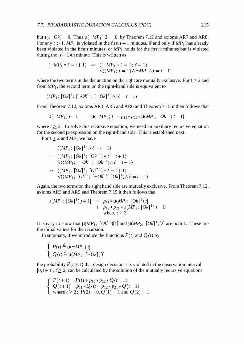
7.7. PROBABILISTIC DURATION CALCULUS (PDC) 215
but τ0(:Ok) = 0. Thus µ(:MP1)[2] = 0, by Theorem 7.12 and axioms AR7 and AR8.For any t > 1, MP1 is violated in the first t+ 1 minutes, if and only if MP1 has alreadybeen violated in the first t minutes, or MP1 holds for the first t minutes but is violatedduring the (t+1)th minute. This is written as
(:MP1 ^ `= t+1) , ((:MP1 ^ `= t); `= 1)_((MP1; `= 1)^:MP1 ^ `= t+1)
where the two terms in the disjunction on the right are mutually exclusive. For t� 2 andfrom MP1, the second term on the right-hand side is equivalent to
(MP1; dOke1; d:Oke1; d:Oke1)^ (`= t+1)
From Theorem 7.12, axioms AR3, AR5 and AR6 and Theorem 7.15 it then follows that
µ(:MP1)[t+1] = µ(:MP1)[t] +p12�p22 �µ(MP1; dOke1)[t�1]
where t � 2. To solve this recursive equation, we need an auxiliary recursive equationfor the second µ-expression on the right-hand side. This is established next.
For t � 2 and MP1 we have
((MP1; dOke1)^ `= t+1)
, ((MP1; dOke1; dOke1)^ `= t+1)_((MP1; d:Oke1; dOke1)^ `= t+1)
, ((MP1; dOke1; dOke1)^ `= t+1)_((MP1; dOke1; d:Oke1; dOke1)^ `= t+1)
Again, the two terms on the right hand side are mutually exclusive. From Theorem 7.12,axioms AR3 and AR5 and Theorem 7.15 it then follows that
µ(MP1; dOke1)[t+1] = p11 �µ(MP1; dOke1)[t]+ p12 �p21 �µ(MP1; dOke1)[t�1]
where t � 2
It is easy to show that µ(MP1; dOke1)[1] and µ(MP2; dOke1)[2] are both 1. These arethe initial values for the recursion.
In summary, if we introduce the functions P (t) and Q (t) by(P (t)
∆= µ(:MP1)[t]
Q (t)∆= µ(MP1; d:Oke)[t]
the probability P (t+1) that design decision 1 is violated in the observation interval[0; t+1], t� 2, can be calculated by the solution of the mutually recursive equations8<:
P (t+1) = P (t)+p12 �p22 �Q (t�1)Q (t+1) = p11 �Q (t)+p12 �p21 �Q (t�1)where t� 2 ; P (2) = 0;Q (1) = 1 and Q (2) = 1
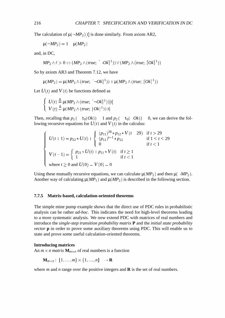
216 CHAPTER 7. SPECIFICATION AND VERIFICATION IN DC
The calculation of µ(:MP2)[t] is done similarly. From axiom AR2,
µ(:MP2) = 1�µ(MP2)
and, in DC,
MP2^ ` > 0, (MP2 ^ (true; d:Oke1))_ (MP2 ^ (true; dOke1))So by axiom AR3 and Theorem 7.12, we have
µ(MP2) = µ(MP2 ^ (true; d:Oke1))+µ(MP2 ^ (true; dOke1))Let U(t) and V (t) be functions defined as(
U(t)∆= µ(MP2 ^ (true; d:Oke1))[t]
V (t)∆= µ(MP2 ^ (true; dOke1))[t]
Then, recalling that p1 (= τ0(Ok)) = 1 and p2 (= τ0(:Ok)) = 0, we can derive the fol-lowing recursive equations for U(t) and V (t) in the calculus:8>>>>>>><>>>>>>>:
U(t+1) = p22 �U(t)+
8<:(p11)
28 �p12 �V (t�29) if t > 29(p11)
t�1 �p12 if 1� t� 290 if t < 1
V (t+1) =
�p21 �U(t)+p11 �V (t) if t� 11 if t < 1
where t� 0 and U(0) = V (0) = 0
Using these mutually recursive equations, we can calculate µ(MP2) and then µ(:MP2).Another way of calculating µ(MP1) and µ(MP2) is described in the following section.
7.7.5 Matrix-based, calculation-oriented theorems
The simple mine pump example shows that the direct use of PDC rules in probabilisticanalysis can be rather ad-hoc. This indicates the need for high-level theorems leadingto a more systematic analysis. We now extend PDC with matrices of real numbers andintroduce the single-step transition probability matrix P and the initial state probabilityvector p in order to prove some auxiliary theorems using PDC. This will enable us tostate and prove some useful calculation-oriented theorems.
Introducing matricesAn m�n matrix Mm�n of real numbers is a function
Mm�n : f1; : : :;mg�f1; : : :;ng �! R
where m and n range over the positive integers and R is the set of real numbers.

7.7. PROBABILISTIC DURATION CALCULUS (PDC) 217
Mm�n is therefore totally determined by assigning a real number mij to Mm�n(i; j) for(i; j) 2 f1; : : :;mg � f1; : : :;ng. Such a matrix is also written as
Mm�n∆=
0B@ m11 : : : m1n...
...mm1 : : : mmn
1CAwhere mij is called the (i; j)th element of Mm�n. When there is no confusion, Mm�n willsimply be written as M.
Let Mm�n denote the set of all m� n matrices and M the set of all matrices of realnumbers. Operations on matrices are defined in terms of their elements. For example,the operation of addition ‘+’ on matrices is defined on Mm�n�Mm�n by
(M+M0)(i; j)∆= M(i; j)+M0(i; j)
where (i; j) 2 f1; : : :;mg�f1; : : :;ng.Similarly, multiplication ‘�’ is defined on Mm�n�Mn�m0 by
(Mm�n �M0n�m0)m�m0(i; j)
∆=
n
∑k=1
M(i;k)�M0(k; j)
where (i; j) 2 f1; : : :;mg�f1; : : :;m0g.Predicates of matrices are defined in terms of predicates of their elements. For exam-
ple, equality ‘=’ between two matrices is defined by
Mm�n = M0m0�n0
∆= (m = m0)^ (n = n0)^ (
(m;n)^(i;j)=(1;1)
(M(i; j) = M0(i; j)))
These definitions show that the arithmetic of matrices of real numbers is in first-orderreal arithmetic, which is the basis of the probabilistic calculus.
Auxiliary notationDefinition 7.6 The following notation is needed:
E is the m�m identity matrix (E(i; j) = 1 for i = j and E(i; j) = 0 for i 6= j).1c is the m�1 matrix (column vector) in which all elements are 1.
zi is the 1�m matrix (row vector) of zeros with the ith element changed from 0 to 1.hi is the m�1 matrix (column vector) of zeros with the 1 in the ith element.
I is the index set f1; : : :;mgIi denotes the subset Infig of I where i 2 I.

218 CHAPTER 7. SPECIFICATION AND VERIFICATION IN DC
Probability matrices and some basic theoremsDefinition 7.7 With V = fv1; : : :;vmg (Definition 7.5), the single-step transition prob-ability matrix P is a real m�m matrix defined by
P∆=
0B@ p11 : : : p1m...
...pm1 : : : pmm
1CA where
8><>:pij
∆= τ(vi;vj) (0 � pij � 1)
∑j2I
pij = 1
and the initial state occupation probability vector p is a real 1�m row vector defined by
p ∆= (p1; : : :;pm) where:
8><>:pi
∆= τ0(vi) (0� pi � 1)
∑i2I
pi = 1
The first theorem is well known from the theory of Markov chains.
Theorem 7.17 For t� 0 and with P0 defined to be the identity matrix E:
Pt � 1c = 1c
The theorem states that the sum of each row in the tth power of the single-step transitionprobability matrix is 1.
Exercise 7.7.4 Prove Theorem 7.17.
Definition 7.8 Let p(t) (t � 0) denote the row vector (p(t)1 ; : : :;p(t)m ) defined by p(t) ∆=
p �Pt
The following theorem states that p(t)i is the (unconditional) probability, that the sys-tem occupies state vi after the tth transition. This is also well known from the theory ofMarkov chains, but it is expressed and proved here in terms of PDC.
Theorem 7.18 For t� 0,
(µ(true; dv1e1)[t+1]; : : :;µ(true; dvme1)[t+1]) = p(t)
Proof: We use induction on t:For t = 0, the result follows from axiom AR7 and the fact that
p = (τ0(v1); : : :;τ0(vm))
Assume that the result holds for t = k; then from Theorem 7.15 and the definition of pji,
µ(true; dvie1)[k+2] = ∑j2I
µ(true; dvje1; dvie1)[k+2]
= ∑j2I
µ(true; dvje1)[k+1]� τ(vj;vi)
= ∑j2I
µ(true; dvje1)[k+1]�pji

7.7. PROBABILISTIC DURATION CALCULUS (PDC) 219
By the induction assumption,
µ(true; dvje1)[k+1] = p(k)j
Therefore, for i 2 I,
µ(true; dvie1)[k+2] = ∑j2I
p(k)j �pji
By the rules given in Section 7.7.5, this leads to
(µ(true; dv1e1)[k+2]; : : :;µ(true; dvme1)[k+2]) = p(k) �PBut, by Definition 7.8,
p(k) �P = (p �Pk) �P = p �Pk+1 = p(k+1)
This proves the theorem.2
Theorems 7.17 and 7.18 imply that the initial probability vector p and the single-steptransition probability matrix P are sufficient to determine the distribution p(t). Taken to-gether, the theorems characterize Pt as the t-step transition probability matrix. In thetheory of stochastic processes the elements of Pt, denoted by p(t)ij , are defined by
p(t)ij∆= P [v = vj at time n+ t j v = vi at time n] (t � 0)
The last theorem in this subsection expresses µ(true)[t+1] (known to be 1) explicitlyin terms of p, P and t. The theorem is not very useful for computation, but it provides asemantic background for the subsequent computation-oriented theorems.
Theorem 7.19 For a non-negative integer t,
µ(true)[t+1] = p �Pt � 1c = 1
Exercise 7.7.5 Prove Theorem 7.19.
ExampleFor a two-state system such as the simple mine pump and for a time interval of length 3
µ(true)[3] = (p1;p2) ��
p11 p12p21 p22
�2
��
11
�= p1p11p11+p1p11p12+p1p12p21+p1p12p22+ p2p21p11+p2p21p12+p2p22p21+p2p22p22 = 1
This shows that the matrix expression for µ(true)[t+ 1] can be expanded into a sum ofsymbolic products where each product defines the probability of a unique behaviour oflength t+1 and all such products are represented.
Clearly, the effect of replacing the duration formula true by a more restrictive for-mula D must be to eliminate all products in the sum except those representing behaviourswhich satisfy D. For a simple class of D formulas, this elimination is obtained by replac-ing certain elements in P or p in the matrix expressions by zeros. This is used in thefollowing theorems.

220 CHAPTER 7. SPECIFICATION AND VERIFICATION IN DC
Computation-oriented theoremsThe first theorem is useful for computation of the probability that a transition to a catas-trophic state does not occur (Case a) or does occur (Case b) within the the first t+1 timeunits.
Theorem 7.20 Let ppidenote p with element pi replaced by zero and let Pci denote P
with all elements in column i replaced by zeros; then for a state vi and a non-negativeinteger t:
(a) µ(2:dvie)[t+1] = ppi� (Pci)
t �1c
(b) µ(3dvie)[t+1] = 1�ppi� (Pci)
t �1c
To prove this theorem we need the following lemma.
Lemma 7.3 For a state vi and a non-negative integer t:
(µ(D1)[t+1]; : : :;µ(Dm)[t+1]) = ppi� (Pci)
t
where: for k 2 I, Dk∆= (2:dvie)^ (true; dvke).
According to this lemma, the kth element of the row vector ppi� (Pci)
t is the probabilitythat the system occupies state vk after the tth transition and that state vi does not occurduring the first t+1 time units.
Proof: We use induction on t. For t = 0 we have ppi� (Pci)
t = ppi�E = ppi
. The resultthen follows from AR7 and the fact that
ppi= (τ0(v1); : : :;τ0(vi�1);0;τ0(vi+1); : : :;τ0(vm))
For t� 0, assume that the result holds for t= n. Then for t = n+1 and for the kth elementof the vector:
µ((2:dvie)^ (true; dvke))[n+2] = µ((2:dvie)^ (true; dvke1))[n+2]
= ∑j2I
µ((2:dvie)^ (true; dvje1; dvke1))[n+2]
For k = i this sum is zero by Theorem 7.12 (µ(false) = 0). For k 6= i we can rewrite thesum, denoted Sum, as follows (notice the parentheses!):
Sum = ∑j2I
µ(((2:dvie)^ (true; dvje1)); dvke1)[n+2]
By axiom AR8 we then obtain
Sum = ∑j2I
µ((2:dvie)^ (true; dvje1))[n+1]� τ(vj;vk)
Replacing τ(vj;vk) by pjk and returning to the vector form, this implies:
(µ(D1)[n+2]; : : :;µ(Dm)[n+2]) = (µ(D1)[n+1]; : : :;µ(Dm)[n+1]) �Pci
By the induction assumption, the last expression is equal to
ppi� (Pci)
n �Pci = ppi� (Pci)
n+1
This proves the lemma.
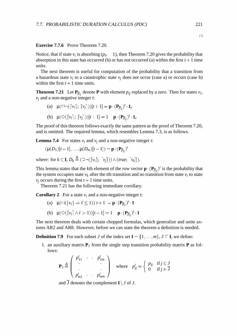
7.7. PROBABILISTIC DURATION CALCULUS (PDC) 221
2
Exercise 7.7.6 Prove Theorem 7.20.
Notice, that if state vi is absorbing (pii = 1), then Theorem 7.20 gives the probability thatabsorption in this state has occurred (b) or has not occurred (a) within the first t+1 timeunits.
The next theorem is useful for computation of the probability that a transition froma hazardous state vi to a catastrophic state vj does not occur (case a) or occurs (case b)within the first t+1 time units.
Theorem 7.21 Let Ppijdenote P with element pij replaced by a zero. Then for states vi,
vj and a non-negative integer t:
(a) µ(2:(dvie; dvje))[t+1] = p � (Ppij)t �1c
(b) µ(3(dvie; dvje))[t+1] = 1�p � (Ppij)t �1c
The proof of this theorem follows exactly the same pattern as the proof of Theorem 7.20,and is omitted. The required lemma, which resembles Lemma 7.3, is as follows.
Lemma 7.4 For states vi and vj and a non-negative integer t:
(µ(D1)[t+1]; : : :;µ(Dm)[t+1]) = p � (Ppij)t
where: for k 2 I, Dk∆= (2:(dvie; dvje))^ (true; dvke).
This lemma states that the kth element of the row vector p � (Ppij)t is the probability that
the system occupies state vk after the tth transition and no transition from state vi to statevj occurs during the first t+1 time units.
Theorem 7.21 has the following immediate corollary.
Corollary 2 For a state vi and a non-negative integer t:
(a) µ(2(dvie ) `� 1))[t+1] = p � (Ppii)t �1
(b) µ(3(dvie^ ` > 1))[t+1] = 1�p � (Ppij)t �1
The next theorem deals with certain chopped formulas, which generalize and unite ax-ioms AR2 and AR8. However, before we can state the theorem a definition is needed.
Definition 7.9 For each subset J of the index set I = f1; : : :;mg, J � I, we define:
1. an auxiliary matrix PJ from the single step transition probability matrix P as fol-lows:
PJ∆=
0BB@p011 � � p01m� �� �
p0m1 � � p0mm
1CCA where p0ij =
�pij if j 2 J0 if j 2 J
and J denotes the complement In J of J.

222 CHAPTER 7. SPECIFICATION AND VERIFICATION IN DC
2. a composite state VJ as follows:
vJ∆=_j2J
vj
Notice that, according to the definition of vJ, (dvJe^ `= t) represents any sequence
(dvj1e1; dvj2e1; : : :dvjte1)
of elementary states of duration 1 such that ji 2 J for i 2 f1; : : :; tg.The theorem makes use of the auxiliary row vector zi and column vector 1c from Def-
inition 7.7.5.
Theorem 7.22 For an arbitrary index set J � I, an arbitrary duration formula D and anarbitrary state vi 2 V
(a) µ(D^ (true; dvie)^ (`= k); dvJe)[t+ k+1]= µ(D^ (true; dvie)[k] � zi � (PJ)
t+1 �1c)
(b) µ(D^ (true; dvie)^ (`= k); 3dvJe)[t+ k+1]= µ(D^ (true; dvie)[k] � (1� zi � (PJ)
t+1 �1c)
To prove this theorem, the following notation and lemma are useful:
q∆= µ(D^ (true; dvie))[k]
and for j 2 I
qj[t]∆=
�µ((D^ (true; dvie)^ (` = k); dvJe)^ (true; dvje))[t+ k+1] if j 2 J0 if j 2 J
We first present the lemma below.
Lemma 7.5 For q and qj[t] as defined above,
(q1[t]; : : :;qm[t]) = q � zi � (PJ)t+1
Exercise 7.7.7 Prove Lemma 7.5 and Theorem 7.22(a).
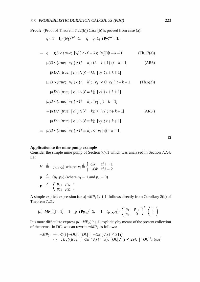
7.7. PROBABILISTIC DURATION CALCULUS (PDC) 223
Proof: (Proof of Theorem 7.22(b)) Case (b) is proved from case (a):
q � (1�1i � (PJ)t+1 �1c = q�q �1i � (PJ)
t+1 �1c
= q�µ(D^ (true; dvie)^ (`= k); dvJe)[t+ k+1] (Th.17(a))
= µ(D^ (true; dvie)^ (` = k); (`= t+1))[t+ k+1] (AR6)
�µ(D^ (true; dvie)^ (` = k); dvJe)[t+ k+1]
= µ(D^ (true; dvie)^ (` = k); dvJe_3dvJe)[t+ k+1] (Th.6(3))
�µ(D^ (true; dvie)^ (` = k); dvJe)[t+ k+1]
= µ(D^ (true; dvie)^ (` = k); dvJe)[t+ k+1]
+µ(D^ (true; dvie)^ (` = k); 3dvJe)[t+ k+1] (AR3 )
�µ(D^ (true; dvie)^ (` = k); dvJe)[t+ k+1]
= µ(D^ (true; dvie)^ (` = k); 3dvJe)[t+ k+1]
2
Application to the mine pump exampleConsider the simple mine pump of Section 7.7.1 which was analyzed in Section 7.7.4.Let
V∆= fv1;v2g where: vi
∆=
�Ok if i = 1:Ok if i = 2
p ∆= (p1;p2) (where p1 = 1 and p2 = 0)
P ∆=
�p11 p12p21 p22
�A simple explicit expression for µ(:MP1)[t+1] follows directly from Corollary 2(b) ofTheorem 7.21:
µ(:MP1)[t+1] = 1�p � (Pp22)t �1c = 1� (p1;p2) �
�p11 p12p21 0
�t
��
11
�It is more difficult to express µ(:MP2)[t+1] explicitly by means of the present collectionof theorems. In DC, we can rewrite :MP2 as follows:
:MP2 , 3((d:Oke; eOke; d:Oke)^ (` � 31)), 9k : ((true; d:Oke)^ (` = k); dOke^ (`� 29); d:Oke1; true)

224 CHAPTER 7. SPECIFICATION AND VERIFICATION IN DC
For a given t, µ(:MP2)[t] is non-zero only if t� k+h+1, where k � 1 and 1� h� 29.Introducing
hmax = min((t� k�1);29)
we can express µ(MP2)[t] by a double summation over all possible ks and hs (this is be-cause we can treat the existential quantification as a disjunction over all possible ks andhs in which the disjuncts are mutually exclusive):
µ(:MP2)[t](by AR6)
=t�2
∑k=1
hmax
∑h=1
µ(true; d:Oke)^ (` = k); dOke^ (` = h); d:Oke1[k+h+1]
(by Theorem 7.22 and Definition 7.7.5)
=t�2
∑k=1
hmax
∑h=1
µ(true; d:Oke)^ (` = k); dOke^ (` = h))[k+h] � (z1 �Pf2g �1c)
(by Theorem 7.22 again)
=t�2
∑k=1
hmax
∑h=1
µ(true; d:Oke)[k] � (z2 �Phf1g �1c) � (z1 �Pf2g �1c)
(by Theorem 7.18, Definition 7.7.5 and Definition 7.7.5)
=t�2
∑k=1
hmax
∑h=1
(p �Pk�1 �h2) � (z2 �Phf1g �1c) � (z1 �Pf2g �1c)
7.9 Historical background
The motivation for DC originally came from the gas burner problem which was chosenas the main case study of the ProCoS project (Bjørner et al., 1993; He et al., 1994). Itwas then realized that control engineers use the properties of integrals and differentials offunctions widely in the description of requirements and for reasoning about the designsof embedded systems. For example, the case study was required to formulate the safetyrequirement of the gas burner in terms of variables denoting undesirable but unavoid-able states such as Leak, which represents the flow of unlit gas from the nozzle: ‘Theproportion of time when gas leaks is not more than one twentieth of the elapsed time, ifthe system is observed for more than one minute’.
A direct formulation of this requirement can be obtained using mathematical analysis;for any interval [b;e] of the real-numbers:
(e�b)� 60) 20R e
bLeak(t)dt � (e�b)
where Leak is a boolean valued step-function from the real-numbers (representing time).But at the time of the start of the ProCoS project no calculus, apart from set theory, wasavailable to express and reason about the properties of integrals or differentials of func-tions. Set theory is far too rich and thus difficult to use for system designs.

7.10. FURTHER WORK 225
Working on the formalization of integrals of boolean-valued functions, Zhou et al.(1991a) developed the duration calculus. Integrals were considered as curried functionsfrom state functions and intervals to real numbers:R
: S! (I! R)
where S denotes the set of states (i.e. boolean-valued step-functions) and I the set ofbounded intervals of real numbers. Moszkowski’s ITL (1985), which uses a discrete timedomain and was developed for reasoning about hardware was extended with continuoustime and then adopted as the base logic for DC. Interval functions such as
RP and
RQ
then become interval variables of ITL.As we have seen in this chapter, DC is a logic for formalizing and reasoning about a
system’s functional and safety properties. It does not provide the means for specifyingand reasoning about the reliability properties of an implementation in which imperfectcomponents are used. Since perfect components are not used in practice, and there is noperfect implementation, there is a need for an extension to deal with probabilities. Liuet al. (1993c) described a probabilistic duration calculus which is a modal logic aboutprefix time intervals; this did not need reference to the time variable t in a probabilisticterm µ(D). The same authors developed a first-order logic (Liu et al., 1994b) for thecalculation of µ(D)[t] and this is the version presented in Section 7.7.
Liu et al. (1993c; 1994b) assume discrete time and model an imperfect implementa-tion as a finite automaton with fixed history, independent of the transition probabilities.This makes discrete Markov processes appropriate as the basis for the calculus. In com-parison with Liu et al. (1993c), the first-order logic in Liu et al. (1994b) is easier to un-derstand and can be used without loss of expressiveness; the latter also gives more detailsand adds computation-oriented theorems to the theory, making the calculus more mech-anizable and also more accessible to reliability engineers.
7.10 Further work
After its initial development, there has been considerable further research on DC: theo-retical developments of the calculus, extensions and application-related work.
7.10.1 Theoretical work
Assuming finite variability of states, a formal semantics of DC was given in Hansen andZhou (1992). Based on this semantics, they also proved that the axioms and rules pre-sented here in Section 7.5 constitute a relatively complete calculus for DC. Results ondecidability and undecidability of DC have appeared in Zhou et al. (1993a) and a proto-type mechanized proof assistant has been implemented by coding the semantics of DC inthe logic of PVS (Skakkebæk & Shankar, 1994). An efficient model checking algorithmfor linear duration invariants has been given in Zhou et al. (1994). An overview on DCand its extensions can be found in Zhou (1993).
226 CHAPTER 7. SPECIFICATION AND VERIFICATION IN DC
For PDC, parallel composition of (open) probabilistic automata is defined in Liu et al.(1993a; 1993b). There, refinement of a probabilistic automata into another through par-allel composition (or decomposition) is formalized, and some compositional proof rulesin terms of PDC are investigated. PDC has been extended by Dang and Zhou (1994) forcontinuous time.
7.10.2 Extensions
The basic DC has several extensions, among which are the probabilistic calculi of Liuet al. (1993c; 1994b). Another extension, called the Extended Duration Calculus (Zhouet al., 1993b), was designed for the specification and verification of hybrid systems whichinclude continuous and discrete states. Here, the arguments of the lifting operator d�e aregeneralized to allow not only boolean-valued functions but also properties like equalityand inequality (we have already seen these used in the mine pump example), continuity,etc. For example, with formulas like dContinous(v)e it is possible to assert that functionv is continuous in an interval and with dv = 0e to assert that v is stable (or constant) inan interval.
Ravn (1994) uses DC and its extensions to investigate both fundamental and practi-cal issues involved in the formal development of embedded real-time systems, includinghybrid systems. The paper links DC to the mathematical analysis of continuous func-tions by allowing the initial and final values, b.f and e.f , of a function f to be defined,as well as its duration
Rf over an interval. The basic DC has also been extended to the
Mean Value Calculus (Zhou & Xiaoshan, 1994) by replacing integrals of boolean-valuedfunctions with their mean values. In this extended calculus, both durations of states andpoint values of states can be expressed, and the latter become significant when a state-based system requirement is to be refined into a communication-based set of components,because communications are instant actions.
The basic DC and these extensions are restricted to finite intervals and use the chopoperator as the only means of contracting subintervals to a given interval. The restric-tion prevents the use of DC for specifying unbounded liveness and fairness properties,such as two users who are served so fairly that they have exactly equal service durations.To accommodate unbounded liveness and fairness, several extensions to DC have beenproposed. The first approach to extending DC for specifying unbounded liveness andfairness was to introduce expanding modalities in DC, while keeping the restriction offinite intervals. Pandya (1994) defined two weakest inverses of the chop operator. En-gel and Rischel (1994) generalized the chop operator by introducing backward intervals.Based on Venema’s (1991) interval temporal logic Skakkebæk (1994) added two expand-ing modalities into DC, which are symmetric and designated as . and /. An interval sat-isfies D1 .D2 iff there exists c such that c� b, [a;c] satisfies D1 and [b;c] satisfies D2.
Although these extensions can express liveness and fairness properties, they are stillunable to differentiate syntactically between a finite and an infinite system behaviour.An infinite behaviour determines a system eternally, while a finite behaviour determinessystem states up to some moment in time, possibly allowing arbitrary continuation. It is
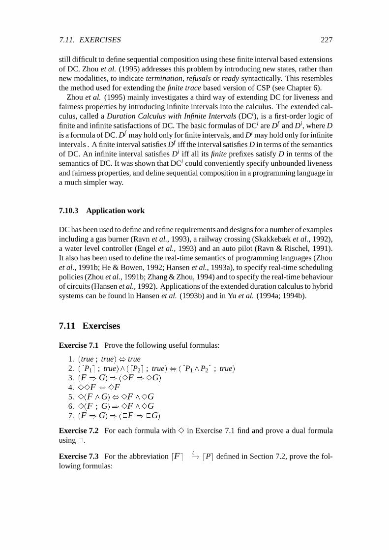
7.11. EXERCISES 227
still difficult to define sequential composition using these finite interval based extensionsof DC. Zhou et al. (1995) addresses this problem by introducing new states, rather thannew modalities, to indicate termination, refusals or ready syntactically. This resemblesthe method used for extending the finite trace based version of CSP (see Chapter 6).
Zhou et al. (1995) mainly investigates a third way of extending DC for liveness andfairness properties by introducing infinite intervals into the calculus. The extended cal-culus, called a Duration Calculus with Infinite Intervals (DCi), is a first-order logic offinite and infinite satisfactions of DC. The basic formulas of DCi are Df and Di, where Dis a formula of DC. Df may hold only for finite intervals, and Di may hold only for infiniteintervals . A finite interval satisfies Df iff the interval satisfies D in terms of the semanticsof DC. An infinite interval satisfies Di iff all its finite prefixes satisfy D in terms of thesemantics of DC. It was shown that DCi could conveniently specify unbounded livenessand fairness properties, and define sequential composition in a programming language ina much simpler way.
7.10.3 Application work
DC has been used to define and refine requirements and designs for a number of examplesincluding a gas burner (Ravn et al., 1993), a railway crossing (Skakkebæk et al., 1992),a water level controller (Engel et al., 1993) and an auto pilot (Ravn & Rischel, 1991).It also has been used to define the real-time semantics of programming languages (Zhouet al., 1991b; He & Bowen, 1992; Hansen et al., 1993a), to specify real-time schedulingpolicies (Zhou et al., 1991b; Zhang & Zhou, 1994) and to specify the real-time behaviourof circuits (Hansen et al., 1992). Applications of the extended duration calculus to hybridsystems can be found in Hansen et al. (1993b) and in Yu et al. (1994a; 1994b).
7.11 Exercises
Exercise 7.1 Prove the following useful formulas:
1. (true ; true), true2. (dP1e ; true)^ (dP2e ; true), (dP1^P2e ; true)3. (F ) G)) (3F )3G)4. 33F ,3F5. 3(F ^G),3F ^3G6. 3(F ; G))3F ^3G7. (F ) G)) (2F )2G)
Exercise 7.2 For each formula with 3 in Exercise 7.1 find and prove a dual formulausing 2.
Exercise 7.3 For the abbreviation dF e t�! dPe defined in Section 7.2, prove the fol-lowing formulas:

228 CHAPTER 7. SPECIFICATION AND VERIFICATION IN DC
1
1 1
1�p
r
p1
e
s mb
Figure 7.8 A protocol over an unreliable medium
1. dPe t�! d:Pe ,2(dPe ) `� t)
2. (dP1e t�! dP2e)^ t � t0) dP1e t0�! dP2e3. (dP1e t1�! dP2e)^ (dP1 ^P2e t1�! dP3e)) dP1e t1+t2�! dP2^P3e4. (dPe c�! d:Pe)^ ((dPe ; d:Pe) �t�c�! d:Pe))2(`� t) RP� c)
Exercise 7.4 Specify a scheduling policy that has an overhead of δ time units whenevera process has to be either placed on a processor for execution or removed from a proces-sor.
Exercise 7.5 Figure 7.8 illustrates a protocol over an unreliable medium which trans-mits a message from a process called Sender to a process called Receiver through a buffer.s, b, m and r are states when the sender, the buffer, the medium and the receiver, respec-tively, are active; e represents the error state of the medium. Calculate the followingprobabilities using the PDC rules:
1. µ(R
r > 0)[t]
2.µ(D1^D2)[t]
µ(D2)[t], where
D1∆= (true; dee)^ (` = k); d:ee^ (` = k1); dee; true
D2∆= (true; dee)^ (` = k); true
Exercise 7.6 Use matrix-based theorems to calculate the probabilities of Exercise 7.5.

Chapter 8
Real-time Systems and Fault-tolerance
Henk Schepers
Introduction
When a component of a computer system fails, it will usually produce some undesir-able effects and it can be said to no longer behave according to its specification. Sucha breakdown of a component is called a fault and its consequence is called a failure. Afault may occur sporadically, or it may be stable and cause the component to fail perma-nently. Even when a fault occurs instantaneously, a fault such as a memory fault mayhave consequences that manifest themselves after a considerable time.
Fault-tolerance is the ability of a system to function correctly despite the occurrenceof faults. Faults caused by errors (or ‘bugs’) in software are systematic and can be repro-duced in the right conditions. The formal methods described in previous chapters addressthe problem of errors in software and, while their use does not guarantee the absence ofsoftware errors, they do provide the means of making a rigorous, additional check. Hard-ware errors may also be systematic but in addition they can have random causes. The factthat a hardware component functions correctly at some time is no guarantee of flawlessfuture behaviour; in Chapter 7, the formal treatment of random faults was described usingthe probabilistic duration calculus. Note that hardware faults often affect the correct be-haviour of software. One of the reasons for introducing dynamic scheduling (see Chapter4) is to deal with the unexpected computational load imposed when faults do occur.
Of course, it is not possible to tolerate every fault. A failure hypothesis stipulates howfaults affect the behaviour of a system. An example of a failure hypothesis is the assump-tion that a communication medium might corrupt messages. With triple modular redun-dancy, a single component is replaced by three replicas and a voter that determines theoutcome, and the failure hypothesis is that at any time at most one replica is affected byfaults. A failure hypothesis divides abnormal behaviour, i.e. behaviour that does not con-form to the specification, into exceptional and catastrophic behaviours. Exceptional be-haviour conforms to the failure hypothesis and must be tolerated, but no attempt need bemade to handle catastrophic behaviour (and, indeed, no attempt may be possible). For ex-ample, if the communication medium mentioned earlier repeatedly sends the same mes-
229

230 CHAPTER 8. REAL-TIME SYSTEMS AND FAULT-TOLERANCE
sage, then this may be catastrophic for a given fault-tolerance scheme. It is important tonote that ‘normal’ behaviour does not mean ‘perfect’ behaviour: after a time-out occurs,the retransmission of a message by a sender is normal but it may result in two copies ofthe same message reaching its destination. Exceptional and normal behaviours togetherform the acceptable behaviour that the system must tolerate. This chapter is concernedwith the following question: can we reason about acceptable behaviour in the same waythat we reason about normal behaviour?
We shall use the compositional proof method of Chapter 5 for reasoning about accept-able behaviour, and the failure hypothesis of a system will be formalized as a relationbetween its normal and acceptable behaviour. Such a relation will allow us to abstractfrom the precise nature and occurrence of faults and focus on the abnormal behaviourthat might be caused. This will lead us to a proof rule by which a specification of the ac-ceptable behaviour can be obtained from the specification of the normal behaviour and apredicate characterizing the failure hypothesis. Given a failure hypothesis χ, Poχ standsfor ‘P under χ’ and means execution of process P under the assumption χ. The accept-able behaviour of process P under the failure hypothesis χ is the normal behaviour of thefailure prone process Poχ.
Use of the method will be demonstrated on the mine pump problem. We shall describehow each component can be affected by malfunctions and then devise ways to toleratethe failures. Because we have to be particularly careful, shifts might be missed unneces-sarily. However, we shall prove that the resulting system is safe, i.e. it will not cause anexplosion.
8.1 Assertions and correctness formulae
Let R be a special variable referring to the timed occurrence function (see Section 5.1.2)which denotes the observable behaviour of a real-time system. Let MVAR be a set oflogical variables with typical element M ranging over timed occurrence functions. Theboolean primitive O@texp will be considered as an abbreviation of O 2 R(texp). In ad-dition, the boolean primitive O@M texp will be used as an abbreviation of O 2M(texp)and similarly we shall use P during M I � 8t 2 I � P@M t, and P inM I � 9 t2 I � P@M t.
Since R refers to all observables, the unrestricted occurrence of R in assertions leadsto problems when trying to apply the parallel composition rule.
Definition 8.1 (Event projection) If E is a set of observable events and ρ is a mapping,the restriction ρ # E of ρ to E at time τ is
(ρ # E)(τ) = ρ(τ)\E
3
Define obs(R # E) = E.
Definition 8.2 (Interval projection) For an interval I � TIME and a mapping ρ, ρ # I isthe restriction of ρ with respect to I and is defined as

8.1. ASSERTIONS AND CORRECTNESS FORMULAE 231
(ρ # I)(τ) =�
ρ(τ) if τ 2 Iø if τ 62 I
�3
Let x0 denote the initial state value of a variable x and let now now0 denote the startingtime. Then instead of
hhx = v� 0 ^ now = t < ∞iiSQRT hhx =p
v ^ t+3� now < t+5ii
we may write, using now0 to refer to the starting time
hhx0 � 0 ^ now0 < ∞iiSQRT hhx =p
x0 ^ now0 +3� now < now0 +5ii
Let var(ϕ) denote the program variables in ϕ and var0(ϕ) the variables x 2 VAR suchthat x0 appears in φ. An assertion will be interpreted with respect to a 4-tuple (σ0;σ;ρ;γ).The state σ0 gives now0 and the terms x0 their value; the state σ, the mapping ρ and theenvironment γ are as defined in Chapter 5. The most important cases are:
� V [[now0]](σ0;σ;ρ;γ) = σ0(now)� V [[x0]](σ0;σ;ρ;γ) = σ0(x)� V [[R]](σ0;σ;ρ;γ) = ρ� V [[M]](σ0;σ;ρ;γ) = γ(M) for M 2MVAR
Furthermore,
� (σ0;σ;ρ;γ) j= 9M � ϕ iff there is some bρ such that (σ0;σ;ρ; (γ : M 7! bρ)) j= ϕ
and if var0(ϕ) =ø then (σ0;σ;ρ;γ) j=ϕ iff (σ;ρ;γ) j=ϕ according to the definition (Sec-tion 5.2.3).
These additions lead to a slightly different definition of the validity of a correctnessformula.
Definition 8.3 (Valid correctness formula) If X 2 VAR� is the list of all variables x 2var(A) and X0 is the corresponding list of terms x0, the correctness formula hhAiiP hhCiiis valid, j= hhAiiP hhCii, iff for all γ and σ0 and any σ and ρ with (σ;ρ) 2M [[P]](σ0):
(σ0;σ;ρ;γ) j= A[X0=X;now0=now]! C
3
If var0(C) = ø then this reduces to the original definition. In this chapter, all programvariables are assumed to be local.

232 CHAPTER 8. REAL-TIME SYSTEMS AND FAULT-TOLERANCE
8.2 Formalizing a failure hypothesis
A failure hypothesis χ of program P is a predicate relating the normal and acceptableexecutions of P. To define such a predicate, we extend the assertion language with thespecial variables nownml and Rnml, and associate with each term x the term xnml.
R, now and x refer to an observation of P, possibly afflicted by faults. Since our taskis to show that a system tolerates the abnormal behaviour of its components to the ex-tent expressed by the failure hypothesis, R, now and x refer to an observation of P that isacceptable with respect to χ.
On the other hand, Rnml, nownml and xnml refer to a normal observation of P. For ex-ample, xnml refers to the value of the program variable x in the final state of a normalexecution, while x denotes its value in the final state of an acceptable execution. Notethat the state in which an execution is started is not affected by faults occurring later inthe execution.
For instance, consider the program INC : x := x+1, which may be subject to a stuck-at-zero-fault in the hardware which does not affect the execution time (i.e. now = nownml)but causes the final value of x to be zero (i.e. x = xnml _ x = 0). This is defined in thefailure hypothesis StuckAtZero.
StuckAtZero � (x = xnml _ x = 0)^ now = nownml ^ R = Rnml
Note: This formalization does not depend on what the final value of x ought to be. 3
If the mapping R has x as an observable, the clause R=Rnml will be unrealistic. In sucha case, the failure hypothesis should show that there may be a time during the executionat which x becomes and remains zero. As mentioned before, in this chapter program vari-ables are not observable.
Note: We shall assume that communication channels and lines are not prone to failureand that the axiomatization of their properties, given in Chapter 5, still applies. 3
Sentences of the extended assertion language are called transformation expressions,typically denoted by ψ. Let varnml(ψ) denote those variables x 2 VAR for which there isa corresponding xnml in ψ. A transformation expression is interpreted with respect to atuple:
(σ0;σnml;σ;ρnml;ρ;γ)
where the state σnml is used to evaluate the terms xnml, the mapping ρnml gives Rnml itsvalue and, as before, the state σ0 is used to evaluate the terms x0, the state σ interpretsthe terms x, the mapping ρ gives R its value and the environment γ interprets the logicalvariables:
� V [[xnml]](σ0;σnml;σ;ρnml;ρ;γ) = σnml(x) for x 2 VAR� V [[x]](σ0;σnml;σ;ρnml;ρ;γ) = σ(x) for x 2 VAR� V [[Rnml]](σ0;σnml;σ;ρnml;ρ;γ) = ρnml
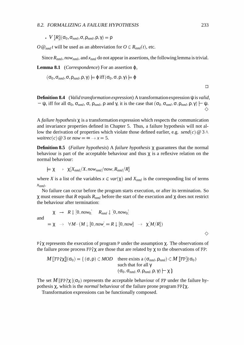
8.2. FORMALIZING A FAILURE HYPOTHESIS 233
� V [[R]](σ0;σnml;σ;ρnml;ρ;γ) = ρ
O@nml t will be used as an abbreviation for O 2 Rnml(t), etc.
Since Rnml, nownml, and xnml do not appear in assertions, the following lemma is trivial.
Lemma 8.1 (Correspondence) For an assertion ϕ,
(σ0;σnml;σ;ρnml;ρ;γ) j= ϕ iff(σ0;σ;ρ;γ) j= ϕ
2
Definition 8.4 (Valid transformation expression) A transformationexpression ψ is valid,j= ψ, iff for all σ0, σnml, σ, ρnml, ρ and γ, it is the case that (σ0;σnml;σ;ρnml;ρ;γ) j= ψ.
3
A failure hypothesis χ is a transformation expression which respects the communicationand invariance properties defined in Chapter 5. Thus, a failure hypothesis will not al-low the derivation of properties which violate those defined earlier, e.g. send(c)@ 3^waitrec(c)@ 3 or now = ∞! x = 5.
Definition 8.5 (Failure hypothesis) A failure hypothesis χ guarantees that the normalbehaviour is part of the acceptable behaviour and thus χ is a reflexive relation on thenormal behaviour:
j= χ ! χ[Xnml=X;nownml=now;Rnml=R]
where X is a list of the variables x 2 var(χ) and Xnml is the corresponding list of termsxnml.
No failure can occur before the program starts execution, or after its termination. Soχ must ensure that R equals Rnml before the start of the execution and χ does not restrictthe behaviour after termination:
j= χ ! R # [0;now0] = Rnml # [0;now0]andj= χ ! 8M � (M # [0;now] = R # [0;now] ! χ[M=R])
3
Poχ represents the execution of program P under the assumption χ. The observations ofthe failure prone process FPoχ are those that are related by χ to the observations of FP:
M [[FPoχ]](σ0) = f (σ;ρ) 2MOD j there exists a (σnml;ρnml) 2M [[FP]](σ0)such that for all γ(σ0;σnml;σ;ρnml;ρ;γ) j= χg
The set M [[FPoχ]](σ0) represents the acceptable behaviour of FP under the failure hy-pothesis χ, which is the normal behaviour of the failure prone program FPoχ.
Transformation expressions can be functionally composed.

234 CHAPTER 8. REAL-TIME SYSTEMS AND FAULT-TOLERANCE
Definition 8.6 (Composite transformation expression) If X 2 VAR� is the list of all x 2VAR such that x 2 var(χ1)\ varnml(χ2), Xnml is the corresponding list of terms xnml andV is a list of fresh logical value variables of the same length as X, then a composite trans-formation expression χ1 oχ2 is
χ1 oχ2 � 9 t;V;M � (χ1[V=X; t=now;M=R]^χ2[V=Xnml; t=nownml;M=Rnml])3
Thus χ1 oχ2 means the application of χ1 and then χ2.Consider the transformation expressions χ1 � (x = xnml_ x = 0)^ (y = ynml_ y = 3)
and χ2 � (y = ynml_ y = 1)^ (z = znml_ z = 2). By definition,
χ1 oχ2 � 9v � (x = xnml_ x = 0)^ (v = ynml_ v = 3)^ (y = v_ y = 1)^ (z = znml_ z = 2)
that is, χ1 oχ2 � (x = xnml_ x = 0)^ (y = ynml_ y = 1_ y = 3)^ (z = znml_ z = 2)The operator χ will also be used to compose assertions and transformation expressions,
e.g. ϕoχ, in commitments. If X 2 VAR� is a list of all x2 varnml(χ), Xnml the correspond-ing list of terms xnml and V is a list of fresh logical value variables of the same length asX, then the composite expression ϕoχ is equivalent to
9 t;V;M � (ϕ[V=X; t=now;M=R]^χ[V=Xnml; t=nownml;M=Rnml])
This replaces all terms xnml that occur in χ by logical value variables. And since ϕ is anassertion, Rnml, nownml and the terms xnml do not appear in ϕ and the composite expres-sion ϕoχ is also an assertion.
Since the interpretation of assertions has not changed, the validity of a correctness for-mula hhAiiFP hhCii remains as defined in Section 8.1.
8.3 A proof rule for failure prone processes
An assumption A may refer to actions that occur during the execution of a program. Sincefaults can affect those occurrences, assumptions should not place restrictions on observ-able events beyond the starting time. Let
NonProphetic(ϕ) � ϕ ! 8M � (M # [0;now] = R # [0;now]! ϕ[M=R])
Then the acceptable behaviour of a process is given in terms of its normal behaviour anda predicate representing the failure hypothesis.
Rule. 8.1 (Failure hypothesis introduction)
hhAiiFP hhCii ; NonProphetic(A)
hhAiiFP oχ hhCoχiiSoundness and completeness of this rule are proved in Section 8.5.

8.3. A PROOF RULE FOR FAILURE PRONE PROCESSES 235
Example 8.1 If the program INC terminates after three and within at most five timeunits, it can be shown that it satisfies
hhnow < ∞iiINC hhx = x0 +1 ^ now0+3 < now < now0+5ii
Since NonProphetic(now < ∞), the failure hypothesis introduction rule gives
hhnow < ∞iiINCoStuckAtZero hh9 t;v � v = x0 +1^now0 +3 < t < now0 +5^ (x = v_ x = 0) ^ now = tii
i.e.
hhnow < ∞iiINCoStuckAtZero hh x = x0 +1_ x = 0^now0 +3 < now < now0 +5ii
Example 8.2 Consider the program F with specification
hhtrueiiF hh8 t < ∞;v� rec(in;v)@t! (:waitsend(out)) during [t; t+Tcomp)^await send(out; f (v))@ t+Tcompii
Suppose, due to faults, that the computation time increases by a factor ∆. For the sakeof simplicity, let us assume that the individual inputs are far enough apart in time not tobe influenced by this (i.e. rec(in;v)@nml t$ rec(in;v)@t). Then, faults only affect thewillingness of the process to perform an out communication, i.e.
(:waitsend(out)) during nml [t1; t2)$ (:waitsend(out)) during [t1; t2+∆)
and
await send(out;v)@nml t$ await send(out;v)@t+∆)
Formally,
Slow�8t < ∞;v � (rec(in;v)@nml t$ rec(in;v)@t)^ 8t1; t2 < ∞�(:waitsend(out)) during nml [t1; t2)
$ (:waitsend(out)) during [t1; t2+∆)^ 8t < ∞;v �awaitsend(out;v)@nml t
$ await send(out;v)@t+∆
Notice that this formalization is transparent to the original computation time and the com-puted function.
Since NonProphetic(true), the failure hypothesis introduction rule yields
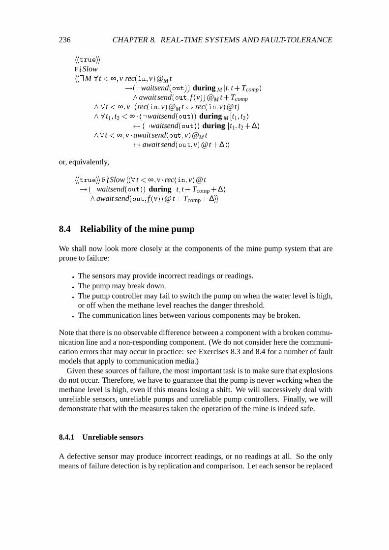
236 CHAPTER 8. REAL-TIME SYSTEMS AND FAULT-TOLERANCE
hhtrueiiFoSlowhh9M�8t < ∞;v�rec(in;v)@M t
!(:waitsend(out)) during M [t; t+Tcomp)^await send(out; f (v))@M t+Tcomp
^ 8t < ∞;v � (rec(in;v)@M t$ rec(in;v)@t)^ 8t1; t2 < ∞ � (:waitsend(out)) during M [t1; t2)
$ (:waitsend(out)) during [t1; t2+∆)^8t < ∞;v �awaitsend(out;v)@M t
$ await send(out;v)@t+∆ii
or, equivalently,
hhtrueiiFoSlowhh8 t < ∞;v � rec(in;v)@t! (:waitsend(out)) during [t; t+Tcomp+∆)^await send(out; f (v))@ t+Tcomp+∆ii
8.4 Reliability of the mine pump
We shall now look more closely at the components of the mine pump system that areprone to failure:
� The sensors may provide incorrect readings or readings.� The pump may break down.� The pump controller may fail to switch the pump on when the water level is high,
or off when the methane level reaches the danger threshold.� The communication lines between various components may be broken.
Note that there is no observable difference between a component with a broken commu-nication line and a non-responding component. (We do not consider here the communi-cation errors that may occur in practice: see Exercises 8.3 and 8.4 for a number of faultmodels that apply to communication media.)
Given these sources of failure, the most important task is to make sure that explosionsdo not occur. Therefore, we have to guarantee that the pump is never working when themethane level is high, even if this means losing a shift. We will successively deal withunreliable sensors, unreliable pumps and unreliable pump controllers. Finally, we willdemonstrate that with the measures taken the operation of the mine is indeed safe.
8.4.1 Unreliable sensors
A defective sensor may produce incorrect readings, or no readings at all. So the onlymeans of failure detection is by replication and comparison. Let each sensor be replaced

8.4. RELIABILITY OF THE MINE PUMP 237
alarmw
alarms
wch
wch1
wch2
wch3
WSens1
WSens2
WSens3
WSVot
Figure 8.1 A triplicate water level sensor
by three sensors, using triple modular redundancy. A ‘voter’ component can then detectonly that a single sensor or its line has failed since these failures will be indistinguishable.
Figure 8.1 shows the resulting system for a water level sensor. Assume that the linebetween the voter and the pump controller can be considered to be fault-free because ofthe short distance. For simplicity, assume that the voter never fails.
An unreliable sensor can:
1. send correct readings, and in time,2. send incorrect readings, but in time, or3. send no readings at all.
(3) occurs also when the sensor that produced incorrect readings is being replaced. Letthe following abbreviations be used for each of these conditions. For k = 1;2;3:
SensOK(wchk)@ t � R # fwchkg(t) = Rnml # fwchkg(t)SensFaulty(wchk)@ t� R # fwchkg(t) = ø ^ :send(wchk)@nml t
_ send(wchk)@ t ^ send(wchk)@nml tSensNC(wchk)@ t � R # fwchkg(t) = ø
Note: These predicates do not exclude each other because it is not always possible to tellwhether or not a device is in sound working order. 3
Then the failure hypothesis UnRel is
UnRel(wchk) � 8t < ∞ � SensOK(wchk)@ t_SensFaulty(wchk)@ t_SensNC(wchk)@ t^wl(t) = wlnml(t)

238 CHAPTER 8. REAL-TIME SYSTEMS AND FAULT-TOLERANCE
(Although this definition is sufficient for our purposes here, it can be easily adapted toexpress quantitative requirements, such as the mean time between failures and the meantime to repair.)
The voter should produce a reading at least once every ∆ws time units. Since votingwill take some time, we require the sensors to send a reading within the first δws timeunits of each ∆ws period, where δws < ∆ws:
WSensC1(wchk) � 8i � send(wchk) in [i∆ws; i∆ws +δws]
As before, we assume that a correct reading does not differ too much from the actuallevel, i.e. that the error is bounded by some value εws:
WSensC2(wchk) � 8t < ∞;v � send(wchk;v)@t! v� εws � wl(t) � v+ εws
Define WSensC(wchk) � WSensC1(wchk)^WSensC2(wchk). Then, for k = 1;2;3,
hhnow = 0iiWSensk hhWSensC(wchk)ii (8.1)
Because no two sensors are identical, their readings may differ slightly, even whentaken at the same time. Assume that the voter WSVot takes the average of the two closestvalues (the so-called inexact voting). If the reading of one sensor differs substantiallyfrom those of the other two, the voter calls for maintenance on the channel alarms byasynchronously sending the identification number of the faulty sensor. Notice that thismethod only works provided the voter receives at least two correct readings in time.
Failure of a sensor reading to arrive may be due to a defective sensor, or a broken line.Given CWSens1, this absence can easily be detected. A call for maintenance can then besent on the channel alarmw.
During the first δws of each ∆ws interval, the voter WSVot is always willing to receiveone reading from each sensor:
WSVotC1 � 8i;k 2 f1;2;3g�waitrec(wchk) during [i∆ws; i∆ws +δws]_ 9 t;v� i∆ws � t < i∆ws +δws
^waitrec(wchk) during [i∆ws; t)^rec(wchk;v)@t^(:rec(wchk)) during (t; i∆ws +δws]
We have to assume that there are at least two correct readings for each vote. Then in-exact voting can be considered as applying a function InexactVote which takes three in-puts. The result part of the outcome is the average of the two values that are closest toeach another; the dissent part is either zero or identifies the value that differs substantiallyfrom the other two. Let the application of the function take TInexactVote time units whichis small enough to guarantee that the voter can produce a reading before the end of the∆ws interval, i.e. δws+TInexactVote is smaller than ∆ws. The voter produces output as soonas possible, i.e.
1. if all three readings get through in time, TInexactVote time units after the last vote isreceived, and
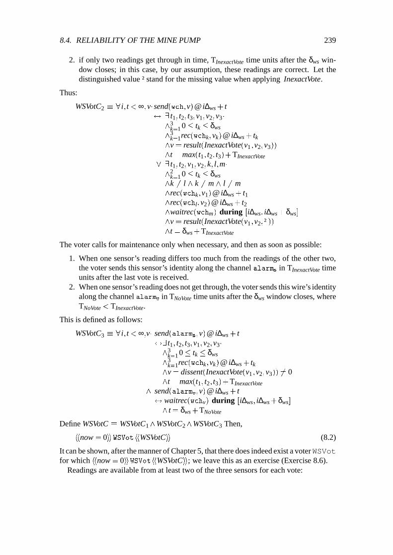
8.4. RELIABILITY OF THE MINE PUMP 239
2. if only two readings get through in time, TInexactVote time units after the δws win-dow closes; in this case, by our assumption, these readings are correct. Let thedistinguished value † stand for the missing value when applying InexactVote.
Thus:
WSVotC2 � 8i; t < ∞;v� send(wch;v)@i∆ws + t$ 9 t1; t2; t3;v1;v2;v3�^3
k=1 0� tk � δws
^3k=1rec(wchk;vk)@ i∆ws + tk^v = result(InexactVote(v1;v2;v3))^t = max(t1; t2; t3)+TInexactVote
_ 9 t1; t2;v1;v2;k; l;m�^2
k=1 0� tk � δws
^k 6= l ^ k 6= m ^ l 6= m^rec(wchk;v1)@ i∆ws + t1^rec(wchl;v2)@ i∆ws + t2^waitrec(wchm) during [i∆ws; i∆ws +δws]^v = result(InexactVote(v1;v2;†))^t = δws +TInexactVote
The voter calls for maintenance only when necessary, and then as soon as possible:
1. When one sensor’s reading differs too much from the readings of the other two,the voter sends this sensor’s identity along the channel alarms in TInexactVote timeunits after the last vote is received.
2. When one sensor’s reading does not get through, the voter sends this wire’s identityalong the channel alarmw in TNoVote time units after the δws window closes, whereTNoVote < TInexactVote.
This is defined as follows:
WSVotC3 � 8i; t < ∞;v� send(alarms;v)@ i∆ws + t$9 t1; t2; t3;v1;v2;v3�^3
k=1 0� tk � δws
^3k=1rec(wchk;vk)@ i∆ws + tk^v = dissent(InexactVote(v1;v2;v3)) 6= 0^t = max(t1; t2; t3)+TInexactVote
^ send(alarmw;v)@ i∆ws + t$ waitrec(wchv) during [i∆ws; i∆ws +δws]^ t = δws +TNoVote
Define WSVotC � WSVotC1^WSVotC2^WSVotC3 Then,
hhnow = 0iiWSVot hhWSVotCii (8.2)
It can be shown, after the manner of Chapter 5, that there does indeed exist a voterWSVotfor which hhnow = 0iiWSVot hhWSVotCii; we leave this as an exercise (Exercise 8.6).
Readings are available from at least two of the three sensors for each vote:

240 CHAPTER 8. REAL-TIME SYSTEMS AND FAULT-TOLERANCE
UnRel�1 �^3k=1 UnRel(wchk)^8i�9k 6= l 2 f1;2;3g�
SensOK(wchk) during [i∆ws; i∆ws +δws]^SensOK(wchl) during [i∆ws; i∆ws +δws]
Note: If one sensor has already been reported as faulty, it would be possible also to tol-erate incorrect readings from another sensor if, for example, the voter selects the morepessimistic of the readings of these two sensors (for the methane level, for instance, thisis the higher reading). 3
The term now does not occur in WSensC(wchk), k = 1;2;3, so by applying the proofrule for parallel composition we obtain from (8.1):
hhnow = 0iiWSens1kWSens2kWSens3 hh^3k=1WSensC(wchk)ii
Clearly, NonProphetic(now = 0). Hence, by the rule for failure hypothesis introduction,we may conclude that
hhnow = 0ii (WSens1kWSens2kWSens3)oUnRel�1 hhUnrelWSensCii (8.3)
where
UnrelWSensC � 9N � (^3k=1WSensC(wchk))[N=R]
^UnRel�1[N=Rnml]
We can now prove that, even in the presence of faults, at least two correct readings areproduced every ∆ws time units.
Lemma 8.2 UnrelWSensC ! 8i � 9k 6= l � (WSC(wchk)^WSC(wchl)) where
WSC(wchk) � send(wchk) in [i∆ws; i∆ws +δws]^ 8t 2 [i∆ws; i∆ws +δws] � send(wchk;v)@t
! v� εws � wl(t) � v+ εws
Proof: Assume UnrelWSensC, i.e. assume that there exists an N such that
(^3k=1WSensC(wchk))[N=R] ^ UnRel�1[N=Rnml] (8.4)
By (^3k=1WSensC(wchk))[N=R], we obtain
8k 2 f1;2;3g � 8 i � send(wchk) inN [i∆ws; i∆ws +δws]^ 8 t < ∞;v � send(wchk;v)@N t
! v� εws � wl(t) � v+ εws
(8.5)
By UnRel�1[N=Rnml], we know that
8i � 9k 6= l � 8 t 2 [i∆ws; i∆ws +δws];v �send(wchk;v)@N t $ send(wchk;v)@t^ send(wchl;v)@N t $ send(wchl;v)@t
(8.6)

8.4. RELIABILITY OF THE MINE PUMP 241
The lemma follows from (8.4), (8.5), and (8.6). 2
By the rule for parallel composition, and (8.3) and (8.2), we know that for
TripleWSens � ((WSens1kWSens2kWSens3)oUnRel�1)kWSVotit is the case that
hhnow = 0iiTripleWSenshhUnrelWSensC^WSVotCiiThe next step is to prove that TripleWSens still produces output at least once every∆ws time units, but that the time taken for voting causes the δws window to increase byTInexactVote time units.
Lemma 8.3 hhnow = 0iiTripleWSenshhWSensC1(wch)[δws +TInexactVote=δws]iiProof: By the consequence rule, we need to prove that
(UnrelWSensC^WSVotC) ! WSensC1(wch)[δws +TInexactVote=δws]
Therefore, assume that UnrelWSensC^WSVotC , or, consequently,
UnrelWSensC^WSVotC1^WSVotC2 (8.7)
By UnrelWSensC and Lemma 8.2, we obtain
8i � 9k 6= l � send(wchk) in [i∆ws; i∆ws +δws]^ send(wchl) in [i∆ws; i∆ws +δws]
By WSVotC1 from (8.7), this leads to
8i � 9k 6= l � rec(wchk) in [i∆ws; i∆ws +δws]^ rec(wchl) in [i∆ws; i∆ws +δws]
(8.8)
Independently of whether or not
^3k=1 rec(wchk) in [i∆ws; i∆ws +δws]
holds for a particular i, we know from WSVotC2 in (8.7) and (8.8) that there exists at� δws +TInexactVote such that send(wch)@i∆ws + t Consequently,
8i � send(wch) in [i∆ws; i∆ws +δws +TInexactVote]
2
The following lemma states that due to delays caused by the voting, the reading errorcan increase by as much as dεws = λmax
in (32δws + TInexactVote).
Lemma 8.4 hhnow = 0iiTripleWSenshhWSensC2(wch)[εws+dεws=εws]ii.Proof: We leave this as an exercise (Exercise 8.7).
Hence, by Lemmas 8.3 and 8.4:
hhnow = 0iiTripleWSenshhWSensC(wch)[ δws+TInexactVote=δws ;εws+dεws=εws]ii
(8.9)
One effect of triple modular redundancy is that it results in less accurate readings. Sincethe original requirement is for at least one reading every ∆ws time units, the increase ofthe δws window is not a problem.

242 CHAPTER 8. REAL-TIME SYSTEMS AND FAULT-TOLERANCE
8.4.2 An unreliable pump
If the pump breaks down while running, the outflow drops to zero within some δbd timeunits. For simplicity, let us assume that δbd equals δp (see Chapter 5). Malfunctioning ofthe pump may also mean that there is no outflow when the pump is activated. Supposethat, due to the space limitations in the mine shaft, the pump cannot be replicated andthat a defective pump must be replaced. During such a replacement, work can continuein the mine until the water level rises above a limit.
One way to monitor the proper functioning of a pump is to look for a reduction in thewater level. But, in practice, the feedback would be too slow to be of much use. So todetect a defective pump we add a water flow sensor to monitor the pump’s outflow. Thissensor is also triplicated.
Failure of the pump to start, or to stop, can be due to a broken control channel. A pumpthat will not stop is a hazard as it can burn out if there is no water to pump, or causean explosion if the methane level is critical. A broken control channel can be detectedindirectly using the water flow sensors.
Typically, a pump is switched on by energizing a relay. To model this, we replace thechannel pch by the line pln (see Section 5.4.3). Let pln(texp) represent the voltage levelof the line pln at time texp. Assume that the line pln is either high (i.e. pln= 1), or low(i.e. pln= 0). Assume also that the voltage level drops to zero if the wire is broken. Thisprovides a fail-safe system: if the wire is broken, the relay is not energized and the pumpstops within δp time units.
Let the maximum outflow of the pump be λmaxout (see Chapter 5):
PumpC1 � 8t < ∞ � 0� outflow(t) < λmaxout
The delays in switching the relay on or off are usually insignificant when compared tothe pump’s reaction time of δp. Consequently, we can safely assume that the pump startswithin δp time units of the line pln becoming high:
PumpC2 � 8t1; t2 < ∞ � pln= 1 during (t1; t2]! outflow� λmin
out during [t1 +δp; t2]
Similarly, assume that the pump stops within δp time units after the line pln becomeslow:
PumpC3 � 8t1; t2 < ∞ � pln= 0 during (t1; t2]! outflow= 0 during [t1 +δp; t2]
We specify that no explosion will occur if the methane level is below the critical levelCML, or if the pump has been switched off (see Chapter 5):
PumpC4 � 8t < ∞ � ml(t) < CML _ 9 t0 � t�δp � pln= 0 during [t0; t]!:expl@t
Let PumpC � PumpC1^PumpC2^PumpC3^PumpC4 . The perfect pump is then de-fined as
hhnow = 0iiPump hhPumpCii (8.10)

8.4. RELIABILITY OF THE MINE PUMP 243
The following lemma, which is easily proved by reductio ad absurdum, states that thepump does not start spontaneously.
Lemma 8.5 j= PumpC!8 t < ∞ � outflow(t) > 0! : (pln= 0 during (t�δp; t])
Define
� PumpOK @ t � outflow(t) = outflownml(t)� PumpNotOK @ t � outflow(t) < outflownml(t) _ outflow(t) = 0
The way in which specification (8.10) is weakened due to the possible occurrence offaults must be defined in a failure hypothesis, and this appears below as NoFlow. First,when a pump breaks down its outflow becomes zero within δp time units. Then, failuredetection and replacement of a defective pump takes at least TRepair time units and thenew pump produces the same outflow as a normal pump within δp time units:
NoFlow � 8t < ∞ � (PumpOK_PumpNotOK)@ t^outflow(t) = outflownml(t)!9 t1 > t � outflow< outflownml during (t; t1)!outflow= 0 during [t+δp; t+δp+TRepair)^ 9 t1 < t � outflow< outflownml during (t1; t)! outflow= 0 during (t�δp�TRepair; t�δp]
^pln(t) = plnnml(t) ^ expl(t) = explnml(t)
Thus, obs(NoFlow) = fexpl;outflow;plng.
Note: This formalization holds for all behaviours, so it may not be illuminating in re-spect of specific behaviours. For example, the pln signal does not change, but there isno indication that a defective or disconnected pump reduces the water level. expl doesnot change because a pump, whether or not it is defective, can cause an explosion if plnis high, indicating that it has not been switched off. 3
Since NonProphetic(now = 0), the failure hypothesis introduction rule yields
hhnow = 0iiPumpoNoFlow hhUnrelPumpCii (8.11)
where
UnrelPumpC � 9N � (PumpC[N=R] ^ NoFlow[N=Rnml])
Although the parameters δp and λminout have little significance for an unreliable pump, the
outflow is still bounded by λmaxout .
Lemma 8.6 j= UnrelPumpC ! 8t < ∞ � 0� outflow(t) < λmaxout

244 CHAPTER 8. REAL-TIME SYSTEMS AND FAULT-TOLERANCE
Proof: Suppose UnrelPumpC, i.e. suppose that there is an N such that
PumpC[N=R] ^ NoFlow[N=Rnml] (8.12)
Since NoFlow[N=Rnml], we may conclude that
8t < ∞ � 0� outflow(t) � outflowN(t) (8.13)
From (8.12), PumpC[N=R], we know PumpC1[N=R], that is,
8t < ∞ � 0� outflowN(t) < λmaxout (8.14)
The lemma follows from (8.13) and (8.14). 2
A more important property to establish is that even an unreliable pump does not startspontaneously.
Lemma 8.7j= UnrelPumpC ! 8t < ∞ � (outflow(t) > 0)!: (pln= 0 during (t�δp; t])
Proof: Assume UnrelPumpC, i.e. assume that there exists an N for which
PumpC[N=R] ^ NoFlow[N=Rnml] (8.15)
Consider anybt such that
outflow(bt )> 0 (8.16)
Since, by (8.15), NoFlow[N=Rnml], we may conclude that
8t < ∞ � outflow(t) � outflowN(t) (8.17)
and
8t < ∞ � pln(t) = plnN(t) (8.18)
By (8.16) and (8.17),
outflowN(bt )> 0 (8.19)
By (8.15), PumpC[N=R]. Consequently, by (8.19) and Lemma 8.5, we may conclude that: (pln= 0 during N (bt �δp;bt ]) , which, by (8.18), yields
: (pln= 0 during (bt �δp;bt ])2
Since faults affect only the outflow, the following lemma is obvious.
Lemma 8.8 UnrelPumpC ! PumpC4

8.4. RELIABILITY OF THE MINE PUMP 245
8.4.3 An unreliable pump controller
The pump controller must monitor the pump’s yield to detect a fault in the pump. Assumethat a sensor FSens sets a line flow to one if there is some outflow from the pump, andto zero otherwise:
FSensC � 8 t < ∞ � (flow(t) = 1 $ outflow(t) > 0)
Assume further that whenever a flow sensor breaks down, the value of the correspondingline drops to zero without delay:
� FSensOK @t � flow(t) = flownml(t)� FSensNotOK @t � flow(t) = 0
The failure hypothesis SensStuckAtZero for the sensor is defined as follows:
SensStuckAtZero � 8t < ∞� (FSensOK_FSensNotOK)@ t^outflow(t) = outflownml(t)
For reliability, the sensor is triplicated, FSensi � FSens[flowi=flow], i= 1;2;3. A voterFVot sets the value of the line flow. Assume that the voting takes exactly TVote timeunits:
FVotC1 �flow= 0 during [0;TVote)^ 8t < ∞ � flow(t+TVote) = Majority(fflowj(t) j j = 1; : : :;3g)
The value of the line flow is either zero or one and, provided that at any time at most onesensor is defective, a line value differing from the majority indicates a defective sensoror a broken wire:
FVotC2 �8t < ∞; i 2 f1;2;3g � send(alarmf; i)@t$flowi 6= Majority(fflowj(t) j j = 1; : : :;3g)@t^ t > 0!9 t1 < t�flowi = Majority(fflowj(t) j j = 1::3g) during [t1; t)
As before, assume that the voter never fails and that at most one sensor is defective atany time:
SensStuckAtZero�1 �^3k=1 SensStuckAtZero[FSensk=FSens;flowk=flow]^8t < ∞ � 9k 6= l�
FSensOK[flowk=flow]@ t^ FSensOK[flowl=flow]@t
In contrast with a single flow sensor FSens, the triple modular redundant flow sensorTripleFSens � ((FSens1kFSens2kFSens3)oSensStuckAtZero�1)kFVot is subject toa delay TVote for the time taken for voting, whether or not faults occur.
Lemma 8.9 hhnow = 0iiTripleFSenshhϕTFSiiwhere

246 CHAPTER 8. REAL-TIME SYSTEMS AND FAULT-TOLERANCE
ϕTFS �flow= 0 during [0;TVote)^ 8t < ∞ � (flow(t+TVote) = 1 $ outflow(t) > 0)
Proof: By the rule for parallel composition, we need to show that
(^3i=1FSensC[flowi=flow])oSensStuckAtZero�1
! 8t < ∞ � (Majority(fflowj(t) j j = 1::3g) = 1 $ outflow(t) > 0)
Therefore, assume (^3i=1FSensC[flowi=flow])oSensStuckAtZero�1 , i.e. that there exists
an N such that (^3i=1FSensC[flowi=flow])[N=R] ^ SensStuckAtZero�1[N=Rnml] Conse-
quently,
(8.20)8t < ∞�outflowN(t) > 0$^3
i=1(flowi)N(t) = 1^ ^3i=1flowi(t) = (flowi)N(t)
_ 9k; l;m � k 6= l 6= m^flowk(t) = (flowk)N(t)^flowl(t) = (flowl)N(t)^flowm(t) = 0 ,
and
8t < ∞ � outflow(t) = outflowN(t) (8.21)
Now consider anybt such that Majority(fflowi(bt ) j i = 1; : : :;3g) = 1 , which, by defini-tion, is the case iff
9k 6= l � (flowk(bt) = 1 ^ flowl(bt ) = 1) (8.22)
By reductio ad adsurdum we conclude from (8.20) and (8.22) that outflowN(bt) > 0 ,which, by (8.21), leads to
outflow(bt )> 0
2
The methane level sensors must also be triplicated. This means that we have also totake into account the possible increase of the methane level during the delay TVote causedby voting:
MSensC � 8 t < ∞ � (mOK(t) = 1 $ ml(t) < SML�TVote λmaxml )
Let MSensi � MSens[mOKi=mOK] for i = 1;2;3. Since, apart from the names of the com-munication lines and channels, the voters MVot and FVot behave identically, define
MVot � FVot[mOKi=flowi]3i=1[alarmm=alarmf]
It is likely that faults affect the sensors MSensandFSens in the same way, i.e.
MSensStuckAtZero�1 � SensStuckAtZero�1[FSensi=MSensi;mOKi=flowi]3i=1
Then the triple modular redundant methane level sensor,
TripleMSens � ((MSens1kMSens2kMSens3)oMSensStuckAtZero�1)kMVotconforms to the original specification in Chapter 5.

8.4. RELIABILITY OF THE MINE PUMP 247
Lemma 8.10 hhnow = 0iiTripleMSenshh8 t < ∞ � (mOK(t) = 1$ ml(t) < SML)iiProof: Exercise 8.8.
For the component MContr we shall copy with the appropriate changes the commit-ments CMC1 through CMC6 from Section 5.5.2. For instance, CMC6 becomes
CMC6 � 8t0; t1� t0+δml � t1^ read(mOK;0)@t0^ (:read(mOK;1)) during [t0; t1]! 9 t2 � t0 +δml � pln= 0 during [t2; t1]
In addition, MContr reads the line flow at least once every ∆read time units:
CMC7 � 8t < ∞ � read(flow) in [t; t+∆read)
If the controller finds that the line flow is low while the line pln has been high for thelast δp +TVote time units, maintenance is notified (by asynchronously sending the valueone along the channel alarmp) after TNoFlow time units, but only once for each periodthat the pump is activated:
CMC8 � 8t� send(alarmp;1)@t+TNoFlow$ 9 t1� t1 < t� (δp +TVote)
^pln(t1) = 0^pln= 1 during (t1; t]^ read(flow;0)@t^ (: send(alarmp)) during (t1; t]
Despite the use of the excellent techniques propagated in this book, it is still possible thatthe pump controller software has errors! It is also possible that the processor executingthe software fails. This can have serious consequences, as a defective pump controllermay not activate the pump when it should begin pumping out water and it may not switchthe pump off when the methane level is critical. This means that incorrect functioning ofthe pump controller should be detected and dealt with as soon as possible.
One way to do this is to duplicate the controller and compare the outputs: the pump canthen be activated only if both controllers agree on the action. For better fault location, itis more sensible to triplicate the controller and use voting to decide on the action.
Assume that the controller software is sufficiently small and simple to be formally ver-ified and checked, and that the processor failure rate is not very high. It may then be ac-ceptable to select a cheaper solution and to use a watchdog timer (cf. Exercise 5.9) whichswitches the pump off unless it is regularly restarted by the controller (see Figure 8.2).This provides a good low-level check for run-away software and provides a fail-safe sys-tem:
CMC9 � 8t < ∞ � send(restart;1) in [t; t+TRestart)
Once again we see that, in comparison with the pump controller presented in Chapter 5,taking the water flow sensor and the watchdog timer into account results in an altogethernew component; the restarting of the timer, for instance, is not the consequence of a fault,but is normal behaviour.
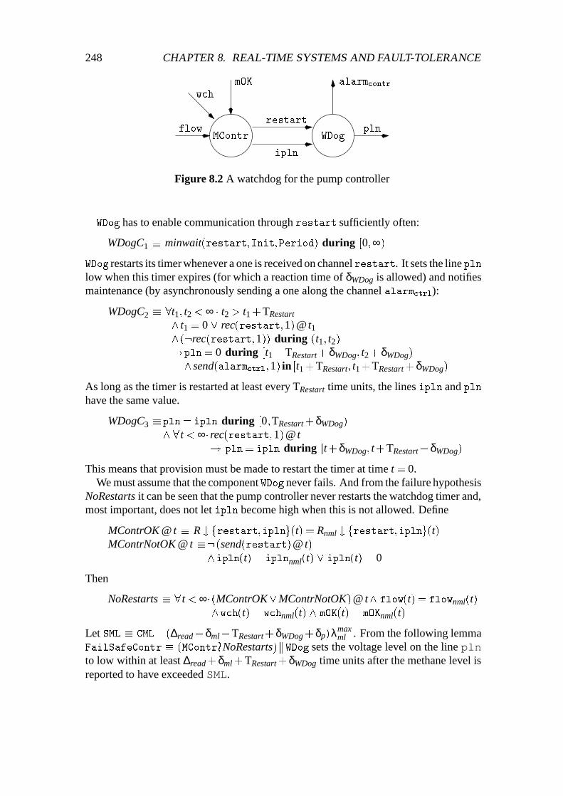
248 CHAPTER 8. REAL-TIME SYSTEMS AND FAULT-TOLERANCE
wch
mOK alarmcontr
flow plnWDog
restart
ipln
MContr
Figure 8.2 A watchdog for the pump controller
WDog has to enable communication through restart sufficiently often:
WDogC1 � minwait(restart;Init;Period) during [0;∞)
WDog restarts its timer whenever a one is received on channel restart. It sets the line plnlow when this timer expires (for which a reaction time of δWDog is allowed) and notifiesmaintenance (by asynchronously sending a one along the channel alarmctrl):
WDogC2 � 8t1; t2 < ∞ � t2 > t1+TRestart
^ t1 = 0 _ rec(restart;1)@t1^ (:rec(restart;1)) during (t1; t2)!pln= 0 during [t1 +TRestart+δWDog; t2+δWDog)^ send(alarmctrl;1) in [t1+TRestart; t1+TRestart +δWDog)
As long as the timer is restarted at least every TRestart time units, the lines ipln and pln
have the same value.
WDogC3 �pln= ipln during [0;TRestart+δWDog)^ 8t < ∞� rec(restart;1)@t
! pln= ipln during [t+δWDog; t+TRestart+δWDog)
This means that provision must be made to restart the timer at time t = 0.We must assume that the component WDog never fails. And from the failure hypothesis
NoRestarts it can be seen that the pump controller never restarts the watchdog timer and,most important, does not let ipln become high when this is not allowed. Define
MContrOK @ t � R # frestart;iplng(t) = Rnml # frestart;iplng(t)MContrNotOK @ t �: (send(restart)@ t)
^ipln(t) = iplnnml(t) _ ipln(t) = 0
Then
NoRestarts � 8t < ∞� (MContrOK_MContrNotOK)@ t^ flow(t) = flownml(t)^wch(t) = wchnml(t) ^ mOK(t) = mOKnml(t)
Let SML � CML� (∆read+δml+TRestart+δWDog+δp)λmaxml . From the following lemma
FailSafeContr � (MControNoRestarts)kWDog sets the voltage level on the line plnto low within at least ∆read+δml +TRestart +δWDog time units after the methane level isreported to have exceeded SML.

8.4. RELIABILITY OF THE MINE PUMP 249
Lemma 8.11 hhnow = 0iiFailSafeContrhhϕFSCii ; where
ϕFSC � 8t0; t1 < ∞� t0+∆read+δml +TRestart+δWDog � t1^mOK= 0 during [t0; t1]! pln= 0 during [t0 +∆read+δml+TRestart+δWDog; t1]
Proof: There are two cases to consider:
(i) If MContrOK during [t0; t0 +∆read + δml] then, according to CMC1, there existst2 (t0 � t2 � t0 +∆read) such that read(mOK;0)@t2, which, by CMC6 (with appro-priate changes), implies that there exists t3 (t0 � t3 � t0+∆read+δml) such that
pln= 0 during [t3; t0+∆read+δml]
Using CMC6 once more, pln normally remains low up to and including t1, so wemay conclude, based on NoRestarts, that
pln= 0 during [t3; t1]
(ii) According to the worst case scenario, MContrOK during [t0; t0+∆read+δml] doesnot hold because MContr fails at t0 +∆read + δml. Also, the timer may not expirebefore t0+∆read+δml +TRestart, and, consequently, pln is not set low before
t0 +∆read+δml +TRestart+δWDog
2
Taking account of the maximum increase in the methane level in the time ∆read+δml+TRestart +δWDog gives the following lemma.
Lemma 8.12hhnow = 0iiFailSafeContrhh8 t < ∞ � ml(t) � CML�δp λmax
ml ! pln(t) = 0ii
8.4.4 A safe mine
In the presence of faults, it can no longer be guaranteed that the water level stays in be-tween the specified lower and higher bounds LWL and HWL, even if the methane levelnever rises above its safe level SML. Let
SafeMine � (PumpoNoFlow)kTripleWSenskTripleFSenskTripleMSenskFailSafeContr
Then it is obviously not true that
hhnow = 0iiSafeMinehh8 t < ∞�ml< SML during [0; t]! LWL< wl(t) < HWLii
But although a number of work-shifts may be lost because the pump fails to operate whenit should, it can be proved that SafeMine is indeed safe.

250 CHAPTER 8. REAL-TIME SYSTEMS AND FAULT-TOLERANCE
Theorem 8.1 hhnow = 0iiSafeMinehh8 t < ∞ � :expl@tiiProof: Two cases need examination:
(i) If ml(t) < CML, then, by Lemma 8.8, not even an unreliable pump can cause anexplosion at time t.
(ii) If ml(t) � CML, then, considering that the methane level increase is at most λmaxml
in unit time, there exists a t0 � t�δp such that ml� CML�δp λmaxml during [t0; t]
Hence, by Lemma 8.12, pln= 0 during [t0; t] ; which, by Lemma 8.8, allows usto conclude that :expl@ t.
2
8.5 Soundness and completeness of the new proof rule
In this section we show that the failure hypothesis introduction rule is sound: in otherwords, if the correctness formula hhAii FP hhCii is derivable, then it is valid. We showalso that the rule is complete: if the correctness formula hhAiiFP hhCii is valid, then it isderivable.
Theorem 8.2 (Soundness) The failure hypothesis introduction rule is sound.
Proof: Assume NonProphetic(A), that is,
j= A ! 8M � (M # [0;now0] = R # [0;now0] ! A[M=R]) (8.23)
and
j= hhAiiFP hhCii (8.24)
Consider any σ0. Let (σ;ρ)2M [[FPoχ]](σ0). Then, from the definition of the semantics,there exists a (σnml;ρnml) 2M [[FP]](σ0) such that, for all γ,
(σ0;σnml;σ;ρnml;ρ;γ) j= χ (8.25)
Since χ is a failure hypothesis,
ρ # [0;σ0(now)] = ρnml # [0;σ0(now)] (8.26)
We must prove hhAiiFP oχ hhCoχii. Assume that, for any γ,
(σ0;σ;ρ;γ) j= A[X0=X;now0=now]
i.e. by (8.23),
(σ0;σ;ρ;γ) j= 8M � M # [0;now0] = R # [0;now0]! A[X0=X;now0=now][M=R]

8.5. SOUNDNESS AND COMPLETENESS OF THE NEW PROOF RULE 251
Let bγ = (γ : M 7! ρnml). By (8.26),
(σ0;σ;ρ;bγ) j= A[X0=X;now0=now][M=R]
By the substitution lemma, we obtain (σ0;σ;ρnml;γ) j= A[X0=X;now0=now]. Since nei-ther now nor any term x appears in A[X0=X;now0=now], this leads to, e.g.
(σ0;σnml;ρnml;γ) j= A[X0=X;now0=now]
Consequently, by (8.24) and the fact that (σnml;ρnml) 2M [[FP]](σ0),
(σ0;σnml;ρnml;γ) j= C
Define bγ = (γ : V 7! σnml(X); t 7! σnml(now);M 7! ρnml). By the substitution lemma(σ0; bσ ; bρ ;bγ) j= C[V=X; t=now;M=R] for any bσ and bρ , for instance
(σ0;σ;ρ;bγ) j= C[V=X; t=now;M=R] (8.27)
By (8.25), we know (σ0;σnml;σ;ρnml;ρ;bγ) j= χ. By the substitution lemma, this obvi-ously leads to (σ0;σnml;σ;ρnml;ρ;bγ) j=χ[V=Xnml; t=nownml;M=Rnml]. Since Rnml, nownmlor any xnml are not in χ[V=Xnml; t=nownml;M=Rnml], the correspondence lemma yields
(σ0;σ;ρ;bγ) j= χ[V=Xnml; t=nownml;M=Rnml] (8.28)
By (8.27) and (8.28),
(σ0;σ;ρ;bγ) j= C[V=X; t=now;M=R] ^ χ[V=Xnml; t=nownml;M=Rnml]
Consequently,
(σ0;σ;ρ;γ) j= 9 t;V;M�(C[V=X; t=now;M=R]^χ[V=Xnml; t=nownml;M=Rnml])
i.e.
(σ0;σ;ρ;γ) j= Coχ
2
As usual when proving completeness, we assume that we can prove any valid formulaof the underlying logic. Thus, using ` ϕ to denote that assertion ϕ is derivable, we addthe following axiom to our proof theory.
Axiom 8.1 (Relative completeness assumption) For an assertion ϕ,
` ϕ if j= ϕ
2
Definition 8.7 (Strongest commitment) An assertion C is called a strongest commit-ment of the assertion A and the failure prone process FP if, and only if,
(i) j= hhAiiFP hhCii , and

252 CHAPTER 8. REAL-TIME SYSTEMS AND FAULT-TOLERANCE
(ii) 8ϕ � ( j= hhAiiFP hhϕii )j= C! ϕ ) .
Using the definition of validity, assertion C is a strongest commitment of A and FP if,and only if,
(i) 8σ0;σ;ρ;γ � (σ0;σ;ρ;γ) j= A[X0=X;now0=now] ^ (σ;ρ) 2M [[FP]](σ0)) (σ0;σ;ρ;γ) j= C ; and
(ii) 8ϕ � 8σ0;σ;ρ;γ � (σ0;σ;ρ;γ) j= A[X0=X;now0=now] ^ (σ;ρ) 2M [[FP]](σ0)) (σ0;σ;ρ;γ) j= ϕ
)j=C! ϕ
Suppose that an assertion sc(A;FP) satisfies
8σ0;σ;ρ;γ � (σ0;σ;ρ;γ) j= A[X0=X;now0=now] ^ (σ;ρ) 2M [[FP]](σ0), (σ0;σ;ρ;γ) j= sc(A;FP)
This stronger version of (i) also satisfies (ii), because for all ψ,
8σ0;σ;ρ;γ � ((σ0;σ;ρ;γ) j= ψ ) (σ0;σ;ρ;γ) j= ϕ) )j= ψ! ϕ
We extend the class of assertions from Section 8.1 to a class of conditions that containsthe strongest commitments. The truth value of a condition with respect to (σ0;σ;ρ;γ) isan extension of the interpretation of assertions with the additional clause
(σ0;σ;ρ;γ) j= sc(A;FP) iff (σ0;σ;ρ;γ) j=A[X0=X;now0=now]and (σ;ρ) 2M [[FP]](σ0)
The next lemma, which follows directly from the definitions, states that sc(A;FP) is asemantic characterization of the strongest commitment of A and FP.
Lemma 8.13 For all ϕ, if j= sc(A;FP)$ ϕ then ϕ is a strongest commitment of A andFP. 2
Observe that a strongest commitment must be an assertion, and hence sc(A;FP) itself isnot a strongest commitment. The following lemma shows how the strongest commitmentof A and FPoχ can be expressed in the case of NonProphetic(A).
Lemma 8.14 If NonProphetic(A) then j= sc(A;FPoχ)$ sc(A;FP)oχ .
Proof: Consider any σ0, σ, ρ and γ and any A such that NonProphetic(A). By the defi-nition of sc, (σ0;σ;ρ;γ) j= sc(A;FPoχ) iff
(σ0;σ;ρ;γ) j= A[X0=X;now0=now]^ (σ;ρ) 2M [[FPoχ]](σ0)
From the definition of the semantics of FPoχ, we obtain (σ0;σ;ρ;γ) j= sc(A;FPoχ) iff
(σ0;σ;ρ;γ) j= A[X0=X;now0=now]^9σnml;ρnml�(σnml;ρnml) 2M [[FP]](σ0)^ (σ0;σnml;σ;ρnml;ρ;γ) j= χ
Equivalently, (σ0;σ;ρ;γ) j= sc(A;FPoχ) iff

8.5. SOUNDNESS AND COMPLETENESS OF THE NEW PROOF RULE 253
9σnml;ρnml � (σ0;σ;ρ;γ) j= A[X0=X;now0=now]^ (σnml;ρnml) 2M [[FP]](σ0)^ (σ0;σnml;σ;ρnml;ρ;γ) j= χ
Observe that
(a) since neither now nor any term x appears in A[X0=X;now0=now],
(σ0;σ;ρ;γ) j= A[X0=X;now0=now]
implies that, for all bσ,
(σ0; bσ ;ρ;γ) j= A[X0=X;now0=now]
(b) by the definition of a failure hypothesis, (σ0;σnml;σ;ρnml;ρ;γ) j= χ implies that
ρ # [0;σ0(now)] = ρnml # [0;σ0(now)]
(c) since NonProphetic(A), and hence NonProphetic(A[X0=X;now0=now]),
(σ0;σ;ρ;γ) j= A[X0=X;now0=now]
implies
(σ0;σ; bρ ;γ) j= A[X0=X;now0=now]
provided bρ # [0;σ0(now)] = ρ # [0;σ0(now)] .
Consequently, (σ0;σ;ρ;γ) j= sc(A;FPoχ) iff
9σnml;ρnml � (σ0;σnml;ρnml;γ) j= A[X0=X;now0=now]^ (σnml;ρnml) 2M [[FP]](σ0)^ (σ0;σnml;σ;ρnml;ρ;γ) j= χ
Then, by the definition of sc, (σ0;σ;ρ;γ) j= sc(A;FPoχ) iff
9σnml;ρnml� (σ0;σnml;ρnml;γ) j= sc(A;FP)(σ0;σnml;σ;ρnml;ρ;γ) j= χ
Hence, (σ0;σ;ρ;γ) j= sc(A;FPoχ) if, and only if, (σ0;σ;ρ;γ) j= sc(A;FP)oχ .2
Now we can establish relative completeness.
Theorem 8.3 (Completeness) The failure hypothesis introduction rule is relatively com-plete.
Proof: Assume that NonProphetic(A). Assume also that
` hhAiiFP hhCSiiwith sc(A;FP)$ CS
Then, by the failure hypothesis introduction rule, we obtain ` hhAiiFP oχ hhCS oχii .
254 CHAPTER 8. REAL-TIME SYSTEMS AND FAULT-TOLERANCE
Suppose j= hhAiiFP oχ hhCii. From sc(A;FP)$ CS and Lemma 8.14, we obtain
j= sc(A;FPoχ)$ CS oχ
Consequently, by Lemma 8.13 and the definition of a strongest commitment,
j= hhAiiFP oχ hhCii leads to j= CS oχ !C
Then, by the relative completeness assumption, ` CS oχ! C.From ` hhAiiFP oχ hhCS oχii and ` CS oχ ! C we obtain, using the consequence rule,
` hhAiiFP oχ hhCii
2
The next lemma states that sc(A;FPoχ) does not impose restrictions on the observablebehaviour after termination; the proof is left as an exercise (Exercise 8.9).
Lemma 8.15j= sc(A;FPoχ)!8M � (M # [0;now] = R # [0;now]! sc(A;FPoχ)[M=R])
8.6 Historical background
Fault-tolerance is the ability of a system to keep functioning correctly, despite faults oc-curring or having occurred (Laprie, 1985). An elaborate overview of many techniques toachieve fault-tolerance can be found in Lee and Anderson (1990). For the greater part,the account in this chapter of the ways of adding to the reliability of the mine pump aretaken from Burns and Lister (1991).
A number of formal methods for dealing with fault-tolerance have been proposed inthe literature. Much of the earlier work on this formalization is state based: in the statemachine approach, the output of several instantiations of a program, each running on adistinct processor, is compared. Lamport’s original description (1978) dealt with fault-free environments only; for a survey of the efforts to generalize the state machine ap-proach to deal with faults see Schneider (1990a). A well-known application of the statemachine approach is the implementation of fail-stop processors (Schlichting & Schnei-der, 1983).
In layered architectures, the exception handling concept (see, e.g. Lee and Anderson,1990) is popular: a layer that provides a service to some higher level layer raises an ex-ception to signal to that layer when a problem is detected that prevents the completionof the requested service, and the higher level layer contains handlers to deal with suchexceptions. In a proof system based on Hoare triples, fpgSfqg, correctness requires thefinal state to satisfy q and Cristian (1985) used Hoare logic to make the normal and ex-ceptional domains of execution explicit by partitioning the initial state space (specifiedby p) into disjoint subspaces for normal and exceptional behaviour by providing a sep-arate specification for each part. Started in the normal subspace the program terminates

8.6. HISTORICAL BACKGROUND 255
normally, but started in the exceptional subspace the program terminates by raising an ex-ception. In Lodaya and Shyamasundar (1990), a proof system is proposed for exceptionhandling in a concurrent program, such as in Ada-like languages.
This kind of fault-tolerance accounts for processor crashes and the effects of faults thatoccur before the invocation of the program. The resulting specifications are often triviallysatisfied by any process that just raises an exception. In Coenen (1993) deontic logicwas proposed to overcome this ‘lazy programmer paradox’. All the same, an unreliablecommunication medium, for instance, does not raise an exception if a message becomescorrupted and simply delivers the bad message.
In the formalisms of Joseph et al. (1987) and He and Hoare (1987) the execution of aprocess restarts as soon as a fault occurs. Hence, a failure prone execution of a process Pconsists of a number of partial executions of P that end in failure followed by a final andcomplete execution. Liu (1991) and Liu and Joseph (1992) describe a framework for rea-soning about programs in the presence of faults and show how program transformationscan be used to derive fault-tolerant behaviour by composing specifications of the fault en-vironment and recovery actions with the program. The incorporation of checkpointingand backward recovery into a program have been investigated in Liu and Joseph (1993;1994) which also contain laws for fault-refinement; Peled and Joseph (1994) contains anextended study of specification and recovery transformations using linear temporal logic.
Processes that crash are studied in Peleska (1991): more precisely, a dual computersystem is proved correct. Such a system contains two replicas of the crash prone process,a ‘master’ and a ‘slave’ which shadows the operation of the master and takes over if andwhen the master crashes. The failure hypothesis in this case stipulates that at least onereplica remains active.
The formalism proposed in Cau and de Roever (1993) allows a program to exhibit ar-bitrary behaviour after a fault occurs. This approach results in conditional specifications:a process behaves according to its specification as long as no faults have occurred. Fault-tolerance is proved by virtue of the system’s failure hypothesis and the available redun-dancy. This approach is not adequate for dealing with the effects of faults that cannotbe masked. For instance, when verifying a system or protocol which employs an errordetecting code it is crucial to be certain that one valid codeword has not been changedinto another.
The effects of faults are taken into account by Weber (1989), where he introduces faultscenarios which are traces that include, besides records of the system’s input and outputoperations, a description of the faults that have occurred. A fault-tolerance property isexpressed as an equivalence between a fault scenario, from which the fault events havebeen removed, and a fault-free trace; this tolerance relation is not elaborated.
In Nordahl (1993), the normal behaviour Soriginal of a system S is distinguished fromits exceptional ‘failure mode’ behaviour Sf . However, it is not possible to derive Sf fromSoriginal and once in failure mode there is no way back. A similar treatment of normaland exceptional behaviour can be found in Coenen and Hooman (1993).
The idea of formalizing a failure hypothesis as a relation between the normal and theacceptable process behaviour was introduced in Schepers (1993). The early attempts to-wards the compositional specification and verification of distributed fault-tolerant sys-

256 CHAPTER 8. REAL-TIME SYSTEMS AND FAULT-TOLERANCE
tems abstract from the internal state of a process as well as the timing of its actions (Schep-ers & Hooman, 1994; Schepers & Coenen, 1995). Consequently, they do not includerules for atomic statements or sequential composition and such proof theories are callednetwork proof theories. Network proof theories for distributed real-time fault-tolerantsystems are given in Schepers and Gerth (1993), where maximal parallelism is assumedand in Schepers (1994), where the limited resources are shared. The proof theory pre-sented in this chapter extends these approaches in that it does take the internal state of aprocess into account.
8.7 Exercises
Exercise 8.1 For a process SORT, where
hhnow = 0iiSORT hhx = min(x0;y0) ^ y = max(x0;y0) ^ now < ∆Sortiiwhich of the following transformation expressions do not qualify as a failure hypothesis,and why?
(a) x0 = 0 ^ y0 = 0(b) now = now0(c) O @ now0�1(d) x = ynml ^ y = xnml(e) now > nownml ^ O @ nownml +5
Exercise 8.2 For a continuously observable variable x, formalize stuck-at-zero memoryfaults.
Exercise 8.3 Consider a transmission medium MEDIUM that waits to (synchronously) ac-cept an input message from a set MSG via a channel in, and within ∆Medium time units en-ables its delivery through the synchronous channel out. Fresh input cannot be accepteduntil the previous message has been delivered.
(a) Specify the normal behaviour of MEDIUM.(b) Formalize omission.(c) Formalize corruption. (Hint: if the failure hypothesis does not restrict the output
values, they are arbitrary.)
Exercise 8.4 Consider the communication medium of Exercise 8.3. In practice, an en-coding function is used to transform a dataword into a codeword which contains someredundant bits. Thus the set of datawords is mapped into a small part of a much largerset of codewords. Codewords to which a dataword is mapped are called valid, and theencoding ensures that it is very unlikely that due to corruption one valid codeword ischanged into another. Formalize this detectable corruption hypothesis. You may assumethat the functions Encode, Decode and Valid are given.

8.7. EXERCISES 257
Exercise 8.5 Consider Figure 8.1. Assume that the channels wch1, wch2 and wch3 arereplaced by media that are prone to detectable corruption, such as the one discussed in theprevious exercise. Design a failure hypothesis that allows that, per vote, at most eitherone sensor or one wire fails.
Exercise 8.6 Show, in the style of Chapter 5, that there exists a voter WSVot such thathhnow = 0iiWSVot hhWSVotCii. You may assume that the function InexactVote is given.
Exercise 8.7 Prove Lemma 8.4. Remember to take into account the effect of a missingor incorrect reading. (Hint: because the voter allows each sensor to communicate at mostone reading for each vote and because channels do not buffer messages, the average oftwo correct readings differs at most by εws+
12δws λmax
in from the water level to which themost recently received reading corresponds. This occurs when the two readings arrive atthe start and the end of the window, respectively, and either both readings are ε too highwhile the water level drops maximally during the interval, or both readings are ε too lowwhile the water level rises maximally.)
Exercise 8.8 Prove Lemma 8.10. (Hint: the proof is similar to that of Lemma 8.9.)
Exercise 8.9 Prove Lemma 8.15.
Exercise 8.10 Show as in Section 8.5, soundness and completeness of the proof rulesof Chapter 5. (Hint: for atomic statements, the strongest commitments follow directlyfrom the relevant axioms and rules, and the non-termination axiom.)


References
Abadi, M., & Lamport, L. 1994. An old-fashioned recipe for real-time. ACM Trans. onProg. Lang. & Syst., 16, 1543–1571.
Alur, R., & Henzinger, T. 1990. Real-time logics: complexity and expressiveness. Pages390–401 of: Proc. Symp. on Logic in Comp. Sc.
Alur, R., Courcoubetis, C., & Dill, D.L. 1990. Model-checking for real-time systems.Pages 414–425 of: Proc. Symp. on Logic in Comp. Sc.
Apt, K.R. 1981. Ten years of Hoare’s logic: a survey – part I. ACM Trans. on Prog.Lang. & Syst., 3, 431–483.
Apt, K.R. 1984. Ten years of Hoare’s logic: a survey – part II: nondeterminism. Th.Comp. Sc., 28, 83–109.
Apt, K.R., Francez, N., & de Roever, W.-P. 1980. A proof system for communicatingsequential processes. ACM Trans. on Prog. Lang. & Syst., 2, 359–385.
Audsley, N.C. 1993. Flexible scheduling in hard real-time systems. Ph.D. thesis, Dept.of Comp. Sc., University of York, UK.
Audsley, N.C., Burns, A., Richardson, M.F., & Wellings, A.J. 1991. Hard real-timescheduling: the deadline monotonic approach. Pages 127–132 of: Proc. 8th IEEEWorkshop on Real-Time Op. Syst. and Softw.
Audsley, N.C., Burns, A., Richardson, M.F., Tindell, K.W., & Wellings, A.J. 1993a. Ap-plying new scheduling theory to static priority pre-emptive scheduling. Softw. Eng.J., 8(5), 284–292.
Audsley, N.C., Burns, A., & Wellings, A.J. 1993b. Deadline monotonic scheduling the-ory and application. J. Control Eng. Pr., 1(1), 71–78.
Audsley, N.C., Burns, A., Davis, R.I., Tindell, K.W., & Wellings, A.J. 1995. Fixed pri-ority scheduling: an historical perspective. J. Real-Time Syst., 8, 173–198.
Baker, T.P. 1990. A stack-based resource allocation policy for realtime processes. In:Proc. 11th IEEE Real-Time Syst. Symp.
Baker, T.P. 1991. Stack-based scheduling of real-time processes. J. Real-Time Syst., 3(1).Barringer, H., Kuiper, R., & Pnueli, A. 1984. Now you may compose temporal logic
specifications. Pages 51–63 of: Proc. 16th ACM Symp. on Theory of Comp.
259

260 REFERENCES
Baruah, S., & Rosier, L.E. 1991. Limitations concerning on-line scheduling algorithmsfor overloaded systems. Pages 128–132 of: 8th IEEE Workshop on Real-Time Op.Syst. and Softw.
Baruah, S., Koren, G., Mao, D., Mishra, B., Rosier, A.R.L., Shasha, D.E., & Wang, F.1992. On the competitiveness of on-line real-time tasks scheduling. J. Real-TimeSyst., 4(2).
Bate, G. 1986. Mascot3: an informal introductory tutorial. Softw. Eng. J., 1(3), 95–102.Bernstein, A.J. 1987. Predicate transfer and timeout in message passing. Inf. Proc. Letts.,
24, 43–52.Bernstein, A.J., & Harter, Jr., P.K. 1981. Proving real-time properties of programs with
temporal logic. Pages 1–11 of: Proc. 8th Annual ACM Symp. on Op. System Prin-ciples.
Berry, G., & Gonthier, G. 1992. The ESTEREL synchronous programming language,design semantics, implementation. Sc. of Comp. Progr., 19(2), 87–152.
Biyabani, S., Stankovic, J.A., & Ramamritham, K. 1988.. The integration of deadlineand criticalness in hard real-time scheduling. In: Proc. 9th IEEE Real-Time Syst.Symp.
Bjørner, D., Langmaack, H., & Hoare, C.A.R. 1993. ProCos I final deliverable. Tech.rept. ID/DTH DB 13/1. Dept. of Comp. Sc., Technical University of Denmark.
Blake, B.A., & Schwan, K. 1991. Experimental evaluation of a real-time scheduler fora multiprocessor system. IEEE Trans. Softw. Eng., 17(1).
Blazewicz, J., Cellary, W., Slowinski, R., & Weglarz, J. 1986. Scheduling under resourceconstraints – deterministic models. Annals of Op. Res., 7.
Bondavalli, A., Stankovic, J.A., & Strigini, L. 1993. Adaptable fault-tolerance for real-time systems. Tech. rept. ESPRIT BRA 6362 Predictably Dependable Comp. Syst.2.
Brookes, S.D., & Roscoe, A.W. 1985. An improved failures model for communicatingsequential processes. In: Proc. Pittsburgh Seminar on Concurrency. LNCS 197.Springer-Verlag.
Brookes, S.D., Hoare, C.A.R., & Roscoe, A.W. 1984. A theory of communicating se-quential processes. J. ACM, 31(7).
Burns, A. 1994. Preemptive priority-based scheduling: an appropriate engineering ap-proach. Pages 225–248 of: Son, S.H. (ed), Advances in Real-Time Systems. PrenticeHall.
Burns, A., & Lister, A.M. 1991. A framework for building dependable systems. Comp.J., 34(2), 173–181.
Burns, A., & Wellings, A.J. 1994. HRT-HOOD: a design method for hard real-time sys-tems. J. Real-Time Syst., 6(1), 73–114.
Burns, A., Lister, A.M., & Wellings, A.J. 1987. A review of Ada tasking. LNCS 262.Springer-Verlag.
Burns, A., Wellings, A.J., Bailey, C.M., & Fyfe, E. 1993. The Olympus attitude andorbital control system: a case study in hard-real-time system design and implemen-tation. Pages 19–35 of: Ada sans frontieres: Proc. 12th Ada-Europe Conf. LNCS688. Springer-Verlag.

REFERENCES 261
Butazzo, G., & Stankovic, J.A. 1993. RED: Robust earliest deadline scheduling. In:Proc. 3rd Intl. Workshop on Resp. Comp. Syst.
Cau, A., & de Roever, W.-P. 1993. Specifying fault-tolerance within Stark’s formalism.Pages 392–401 of: Proc. 23rd Symp. on Fault-Tolerant Comp. IEEE Comp. SocietyPress.
Chetto, H., & Chetto, M. 1989. Some results of the earliest deadline scheduling algo-rithm. IEEE Trans. on Softw. Eng.
Coenen, J. 1993. Top-down development of layered fault-tolerant systems and its prob-lems – A deontic perspective. Annals of Maths. and AI, 9, 133–150.
Coenen, J., & Hooman, J. 1993. Parameterized semantics for fault-tolerant real-timesystems. Pages 51–78 of: Vytopil, J. (ed), Formal Tech. in Real-Time and Fault-Tolerant Syst. Kluwer Academic Publishers.
Coffman, E.G. (ed). 1976. Computer and Job-shop Scheduling Theory. John Wiley &Sons.
Cristian, F. 1985. A rigorous approach to fault-tolerant programming. IEEE Trans. onSoftw. Eng., SE-11(1), 23–31.
Cristian, F., Aghili, H., Strong, R., & Dolev, D. 1989. Atomic broadcast: from simplemessage diffusion to Byzantine agreement. Research Report RJ 5244. IBM AlmadenResearch Center.
Davies, J.W. 1993. Specification and Proof in Real-Time Systems. Cambridge UniversityPress.
Davies, J.W., & Schneider, S.A. 1990. Factorising proofs in timed CSP. In: Proc.5th Intl. Conf. on the Mathematical Foundations of Prog. Semantics. LNCS 442.Springer-Verlag.
Davies, J.W., & Schneider, S.A. 1993. Recursion induction for real-time processes. For-mal Asp. of Comp., 5(6).
Davies, J.W., & Schneider, S.A. 1995. Real-time CSP. In: Rus, T., & Rattray, C. (eds),Theories and Experiences for Real-Time System Development. AMAST Series inComp., vol. 2. World Scientific.
Davies, J.W., Jackson, D.M., & Schneider, S.A. 1992. Broadcast communication for real-time processes. In: Vytopil, J. (ed), Proc. Symp. on Real-Time and Fault-TolerantSyst. LNCS 571. Springer-Verlag.
de Bakker, J. 1980. Mathematical Theory of Program Correctness. Prentice Hall Inter-national.
de Roever, W.-P. 1985. The quest for compositionality – A survey of assertion-basedproof systems for concurrent programs, Part I: Concurrency based on shared vari-ables. Pages 181–207 of: Proc. IFIP Working Conf. 1985: The role of abstractmodels in computer science. North-Holland.
Dertouzos, M.L., & Mok, A.K.-L. 1989. Multiprocessor on-line scheduling of hard-real-time tasks. IEEE Trans. on Softw. Eng., 15(12).
Dijkstra, E.W. 1976. A Discipline of Programming. Prentice Hall.Emerson, E., Mok, A.K.-L., Sistla, A.P., & Srinivasan, J. 1989. Quantitative temporal
reasoning. Workshop On Automatic Verification Methods for Finite State Syst.,Grenoble, France.

262 REFERENCES
Engel, M., & Rischel, H. 1994. Dagstuhl seminar specification problem – a durationcalculus solution. Personal communication.
Engel, M., Kubica, M., Madey, J., Parnas, D.L., Ravn, A.P., & van Schouwen, A.J. 1993.A formal approach to computer systems requirements documentation. Pages 452–474 of: Grossman, R.L., Nerode, A., Ravn, A.P., & Rischel, H. (eds), Hybrid Sys-tems. LNCS 736. Springer-Verlag.
Francez, N., Lehman, D., & Pnueli, A. 1984. A linear history semantics for distributedprogramming. Th. Comp. Sc., 32, 25–46.
Furht, B., Grostick, D., Gluch, D., Rabbat, G., Parker, J., & Roberts, M. 1991. Real-timeUnix Systems. Kluwer Academic Publishers.
Gerber, R., & Lee, I. 1989. Communicating shared resources: a model for distributedreal-time systems. Pages 68–78 of: Proc. 10th IEEE Real-Time Syst. Symp.
Gerber, R., & Lee, I. 1990. CCSR: a calculus for communicating shared resources. Pages263–277 of: CONCUR 90. LNCS 458. Springer-Verlag.
Gibbins, P., Kay, A., & Schneider, S.A. 1993. Asynchronous perceptrons in real-timeCSP. ESPRIT CONCUR2 project deliverable.
Goli, P., Kurose, J., & Towsley, D. 1990. Approximate minimum laxity scheduling al-gorithms for real-time systems. Tech. rept. University of Massachusetts, Amherst,Dept. of Comp. and Inf. Sc.
Goodenough, J.B., & Sha, L. 1988. The priority ceiling protocol: A method for mini-mizing the blocking of high priority Ada tasks. Chap. 8(7), pages 20–31 of: Proc.2nd Intl. Workshop on Real-Time Ada Issues, ACM Ada Letts.
Gudmundsson, O., Mose, D., Ko, K., Agrawala, A., & Tripathi, S. 1992. Maruti, an en-vironment for hard real-time applications. In: Agrawala, A., Gordon, K., & Hwang,P. (eds), Mission Critical Operating Systems. IOS Press.
Haase, V.H. 1981. Real-time behaviour of programs. IEEE Trans. on Softw. Eng., SE-7(5), 494–501.
Hammer, D., Luit, E., van Roosmalen, O., van der Stok, P., & Verhoosel, J. 1994. Dedos:A distributed real-time environment. IEEE Parallel & Distr. Technology, Syst. &Applications, 2(4), 32–47.
Hansen, M.R., & Zhou, C.C. 1992. Semantics and completeness of the duration calculus.Pages 209–225 of: de Bakker, J.W., Huizing, K., de Roever, W.-P., & Rozenberg,G. (eds), Real-time: Theory in Practice, 1991. LNCS 600. Springer-Verlag.
Hansen, M.R., Zhou, C.C., & Staunstrup, J. 1992. A real-time duration semantics forcircuits. In: Proc. 1992 ACM/SIGDA Workshop on Timing Issues in Specificationand Synthesis of Digital Systems. Princeton, NJ, March 18–20.
Hansen, M.R., Olderog, E.-R., Schenke, M., Franzle, M., v. Karger, B., Muller-Olm, M.,& Rischel, H. 1993a. A duration calculus semantics for real-time reactive systems.Tech. rept. OLD MRH 1/1. Oldenburg Universitat.
Hansen, M.R., Pandya, P.K., & Zhou, C.C. 1993b. Finite divergence. Tech. rept. Rep.15. UNU/IIST, Macau.
Hansson, H., & Jonsson, B. 1989. A framework for reasoning about time and reliability.Pages 102–111 of: Proc. IEEE Real-Time Syst. Symp.

REFERENCES 263
Harel, D. 1987. Statecharts: a visual formalism for complex systems. Sc. Comp. Prog.,8, 231–274.
Harel, E. 1988. Temporal analysis of real-time systems. Master’s Thesis. The WeizmannInstitute of Sc., Rehovot, Israel.
Harel, E., Lichtenstein, O., & Pnueli, A. 1990. Explicit clock temporal logic. Pages402–413 of: Proc. Symp. on Logic in Comp. Sc. IEEE.
Harter Jr., P.K. 1987. Response times in level structured systems. ACM Trans. Comp.Sys., 5(3), 232–248.
He, J., & Bowen, J. 1992. Time interval semantics and implementation of a real-time pro-gramming language. In: Proc. 4th Euromicro Workshop on Real-Time Syst. IEEEComp. Society Press.
He, J., & Hoare, C.A.R. 1987. Algebraic specification and proof of a distributed recoveryalgorithm. Distr. Comp., 2, 1–12.
He, J., Hoare, C.A.R., Fanzle, M., Muller-Olm, M., Olderog, E., Schenke, M., Hansen,M.R., Ravn, A.P., & Rischel, H. 1994. Provably correct systems. Pages 288–335of: Langmaack, H., de Roever, W.-P., & Vytopil, J. (eds), Proc. Symp. on FormalTech. in Real-Time and Fault-Tolerant Syst. LNCS 853. Springer-Verlag.
Hehner, E.C.R. 1989. Real-time programming. Inf. Proc. Letts., 30, 51–56.Hoare, C.A.R. 1969. An axiomatic basis for computer programming. Comm. ACM,
12(10), 576–580, 583.Hoare, C.A.R. 1978. Communicating sequential processes. Comm. ACM, 21(8).Hoare, C.A.R. 1985. Communicating Sequential Processes. Prentice Hall International.Holmes, V.P., Harris, D., Piorkowski, K., & Davidson, G. 1987. Hawk: An operating
system kernel for a real-time embedded multiprocessor. Tech. rept. Sandia NationalLabs.
Hong, J., Tan, X., & Towsley, D. 1989. A performance analysis of minimum laxityand earliest deadline scheduling in a real-time systems. IEEE Trans. on Comp.,C-38(12).
Hong, K.S., & Leung, J.Y-T. 1988. On-line scheduling of real-time tasks. In: Proc. 9thIEEE Real-Time Syst. Symp.
Hooman, J. 1987. A compositional proof theory for real-time distributed message pass-ing. Pages 315–332 of: Parallel Architectures and Languages Europe. LNCS 259.Springer-Verlag.
Hooman, J. 1990. Compositional verification of distributed real-time systems. Pages1–20 of: Proc. Workshop on Real-Time Syst. – Theory and Applications. North-Holland.
Hooman, J. 1991. Specification and Compositional Verification of Real-Time Systems.LNCS 558. Springer-Verlag.
Hooman, J. 1993. Specification and verification of a distributed real-time arbitration pro-tocol. Pages 284–293 of: Proc. 14th IEEE Real-Time Syst. Symp.
Hooman, J. 1994a. Compositional verification of a vistributed real-time arbitration pro-tocol. J. Real-Time Syst., 6(2), 173–205.

264 REFERENCES
Hooman, J. 1994b. Correctness of real-time systems by construction. Pages 19–40 of:Langmaack, H., de Roever, W.-P., & Vytopil, J. (eds), Formal Tech. in Real-Timeand Fault-Tolerant Syst. LNCS 863. Springer-Verlag.
Hooman, J., & de Roever, W.-P. 1986. The quest goes on: a survey of proof systemsfor partial correctness of CSP. Pages 343–395 of: Current Trends in Concurrency.LNCS 224. Springer-Verlag.
Hooman, J., & de Roever, W.-P. 1990. Design and verification in real-time distributedcomputing: an introduction to compositional methods. Pages 37–56 of: ProtocolSpecification, Testing and Verification, IX. North-Holland.
Hooman, J., & Widom, J. 1989. A temporal-logic based compositional proof systemfor real-time message passing. Pages 424–441 of: Parallel Architectures and Lan-guages Europe. LNCS 366. Springer-Verlag.
Hooman, J., Kuiper, R., & Zhou, P. 1991. Compositional verification of real-time sys-tems using explicit clock temporal logic. Pages 110–117 of: Proc. 6th Intl. Work-shop on Softw. Specification and Design. IEEE.
Howles, F. 1993. Distributed arbitration in the Futurebus protocol. M.Sc. thesis, OxfordUniversity.
Huizing, C., Gerth, R., & de Roever, W.-P. 1987. Full abstraction of a real-time denota-tional semantics for an OCCAM-like language. Pages 223–237 of: Proc. 14th ACMSymp. on Principles of Prog. Languages.
Hung, D.V., & Zhou, C.C. 1994. Probabilistic duration calculus for continuous time.Tech. rept. UNU/IIST Report 25. UNU/IIST, Macau.
IEEE. 1988. Standard backplane and bus specification for multiprocessor architectures:Futurebus. IEEE.
Jackson, D.M. 1989. The specification of aircraft engine control software in timed CSP.M.Sc. thesis, Oxford University.
Jackson, D.M. 1990. Specifying timed communicating sequential processes using tempo-ral logic. Tech. rept. TR–5–90. Programming Research Group, Oxford University.
Jackson, D.M. 1992. Logical verification of reactive software systems. D.Phil thesis,Oxford University.
Jahanian, F., & Mok, A.K.-L. 1986. Safety analysis of timing properties in real-timesystems. IEEE Trans. on Softw. Eng., SE-12(9), 890–904.
Jensen, D. 1992. The kernel computational model of the Alpha real-time distributed op-erating system. In: Agrawala, A., Gordon, K., & Hwang, P. (eds), Mission CriticalOperating Systems. IOS Press.
Joseph, M. 1985. On a problem in real-time computing. Inf. Proc. Letts, 20(4), 173–177.Joseph, M., & Pandya, P.K. 1986. Finding response times in a real-time system. Comp.
J., 29(5), 390–395.Joseph, M., Moitra, A., & Soundararajan, N. 1987. Proof rules for fault-tolerant dis-
tributed programs. Sc. Comp. Prog., 8, 43–67.Kay, A., & Reed, J.N. 1990. A specification of a telephone exchange in timed CSP. Tech.
rept. TR–19–90. Programming Research Group, Oxford University.
REFERENCES 265
Klein, M.H., Ralya, T.A., Pollak, B., Obenza, R., & Harbour, M.G. 1993. A Practi-tioner’s Handbook for Real-time Analysis: a guide to rate monotonic analysis forreal-time systems. Kluwer Academic Publishers.
Koymans, R. 1990. Specifying real-time properties with metric temporal logic. J. Real-Time Syst., 2(4), 255–299.
Koymans, R. 1992. Specifying Message Passing and Time-Critical Systems with Tem-poral Logic. LNCS 651. Springer-Verlag.
Koymans, R., & de Roever, W.-P. 1985. Examples of a real-time temporal logic specifica-tion. Pages 231–252 of: The Analysis of Concurrent Systems. LNCS 207. Springer-Verlag.
Koymans, R., Vytopyl, J., & de Roever, W.-P. 1983. Real-time programming and asyn-chronous message passing. Pages 187–197 of: Proc. 2nd ACM Symp. on Principlesof Distr. Comp.
Koymans, R., Shyamasundar, R.K., de Roever, W.-P., Gerth, R., & Arun-Kumar, S. 1988.Compositional semantics for real-time distributed computing. Inf. & Comp., 79(3),210–256.
Kramer, J., Magee, J., Sloman, M.S., & Lister, A.M. 1983. CONIC: an integrated ap-proach to distributed computer control systems. Proc. IEE (Part E), 180(1), 1–10.
Lamport, L. 1978. Time, clocks, and the ordering of events in a distributed system.Comm. ACM, 21(7), 558–565.
Lamport, L. 1983. Specifying concurrent program modules. ACM Trans. on Prog. Lang.& Syst., 5(2), 190–222.
Lamport, L. 1993. Hybrid systems in TLA+. Pages 77–102 of: Workshop on Theory ofHybrid Systems. LNCS 736. Springer-Verlag.
Lamport, L. 1994. The temporal logic of actions. ACM Trans. on Prog. Lang. & Syst.,1(3), 872–923.
Lamport, L., & Merz, S. 1994. Specifying and verifying fault-tolerant systems. Pages41–76 of: Langmaak, H., de Roever, W.-P., & Vytopil, J. (eds), Formal Tech. inReal-Time and Fault-Tolerant Syst. LNCS 863. Springer-Verlag.
Laprie, J.C. 1985. Dependable computing and fault-tolerance: concepts and terminology.Pages 2–11 of: Proc. 15th Symp. on Fault-Tolerant Comp. IEEE Comp. SocietyPress.
Lee, P.A., & Anderson, T. 1990. Fault-Tolerance: Principles and Practice. Springer-Verlag.
Lehoczky, J. 1990. Fixed priority scheduling or periodic task sets with arbitrary dead-lines. Pages 201–209 of: Proc. 11th IEEE Real-Time Syst. Symp.
Lehoczky, J., Sha, L., & Ding, Y. 1989. The rate-monotonic scheduling algorithm: exactcharacterisation and average case behavior. Pages 261–270 of: Proc. 10th IEEEReal-Time Syst. Symp.
Leveson, N. 1995. Safeware: System Safety and Computers. Addison-Wesley.Levin, G.M., Gries, D. 1981 A proof technique for communicating sequential processes.
Acta Informatica, 15, 281–302.

266 REFERENCES
Lincoln, P., & Rushby, J. 1993. The formal verification of an algorithm for interactiveconsistency under a hybrid fault model. Pages 292–304 of: Comp. Aided Verif. 93.LNCS 697. Springer-Verlag.
Liu, C.L., & Layland, J.W. 1973. Scheduling algorithms for multiprogramming in a hard-real-time environment. J. ACM, 20(1), 40–61.
Liu, J.W.S., Lin, K., Shih, W., Yu, A., Chung, J., & Zhao., W. 1991. Algorithms forscheduling imprecise calculations. IEEE Comp., 24(5), 58–68.
Liu, J.W.S., Shih, W.K., Lin, K.J., Bettati, R., & Chung, J.Y. 1994. Imprecise computa-tions. In: Proc. IEEE.
Liu, Z. 1991. Fault-tolerant programming by transformations. Ph.D. thesis, Universityof Warwick.
Liu, Z., & Joseph, M. 1992. Transformation of programs for fault-tolerance. FormalAsp. Comp., 4, 442–469.
Liu, Z., & Joseph, M. 1993. Specification and verification of recovery in asynchronouscommunicating systems. Pages 137–165 of: Vytopil, J. (ed), Formal Techiques inReal-Time and Fault-Tolerant Systems Kluwer Academic Publishers.
Liu, Z., & Joseph, M. 1994. Stepwise development of fault-tolerant reactive systems.Pages 529–546 of: Langmaak, H., de Roever, W.-P., & Vytopil, J. (eds), FormalTech. in Real-Time and Fault Tolerant Syst. LNCS 863. Springer-Verlag.
Liu, Z., Nordahl, J., & Sørensen, E.V. 1993a. Composition and refinement of probabilis-tic real-time systems. Pages 31–40 of: Gorski, Janusz (ed), Proc. 12th Intl. Conf.on Comp. Safety, Reliability and Security. Springer-Verlag.
Liu, Z., Nordahl, J., & Sørensen, E.V. 1993b. Compositional design and refinement ofprobabilistic real-time systems. In: IMA Conf. on Maths. of Dependable Syst.
Liu, Z., Ravn, A.P., Sørensen, E.V., & Zhou, C.C. 1993c. A probabilistic duration calcu-lus. Pages 29–52 of: Kopetz, H., & Kakuda, Y. (eds), Responsive Comp. Syst. Dep.Comp. and Fault-Tol. Syst., vol. 7. Springer-Verlag.
Liu, Z., Ravn, A.P., Sørensen, E.V., & Zhou, C.C. 1994b. Towards a calculus of systemsdependability. High Integrity Syst., 1(1), 49–75.
Liu, Z., Joseph, M., & Janowski, T. 1995. Verification of schedulability for real-timeprograms. Formal Asp. of Comp., 7(5), 510–532.
Locke, C.D. 1985. Best-effort decision making for real-time scheduling. Ph.D. thesis,Carnegie-Mellon University, Pittsburgh, PA.
Lodaya, K., & Shyamasundar, R.K. 1990. Proof theory for exception handling in a task-ing environment. Acta Inf., 28, 7–41.
Lowe, G. 1993. Probabilities and priorities in timed CSP. D.Phil thesis, Oxford Univer-sity.
Mahony, B.P., & Hayes, I.J. 1992. A case-study in timed refinement: a mine pump. IEEETrans. on Softw. Eng., 18(9), 817–826.
Manna, Z., & Pnueli, A. 1982. Verification of concurrent programs: a temporal proofsystem. Pages 163–255 of: Foundations of Comp. Sc. IV, Distr. Syst.: Part 2. Math-ematical Centre Tracts, vol. 159.
Mislove, M.W., Roscoe, A.W., & Schneider, S.A. 1995. Fixed points without complete-ness. Th.Comp. Sc., 138.

REFERENCES 267
Mok, A.K.-L. 1983. Fundamental design problems of distributed systems for the hardreal-time environment. Ph.D. thesis, Dept. of Electrical Eng. and Comp. Sc., M.I.T,Cambridge, MA.
Mok, A.K.-L., & Dertouzos, M.L. 1978. Multiprocessor scheduling in a hard real-timeenvironment. In: Proc. 7th Texas Conf. on Comp. Syst.
Moszkowski, B. 1985. A temporal logic for multi-level reasoning about hardware. IEEEComp., 18(2).
Nassor, E., & Bres, G. 1991. Hard real-time sporadic task scheduling for fixed priorityschedulers. Pages 44–47 of: Proc. Intl. Workshop on Responsive Comp. Syst.
Nguyen, V., Demers, A., Gries, D., & Owicki, S. 1986. A model and temporal proofsystem for networks of processes. Distr. Comp., 1(1), 7–25.
Nordahl, J. 1993. Design for dependability. Pages 65–89 of: Dependable Computingand Fault Tolerant Systems, 8. Springer-Verlag.
Olderog, E.R. 1985. Process theory: semantics, specification and verification. Pages509–519 of: ESPRIT/LPC Advanced School on Current Trends in Concurrency.LNCS 194. Springer-Verlag.
Ostroff, J. 1989. Temporal Logic for Real-Time Systems. Advanced Softw. DevelopmentSeries. Research Studies Press.
Owicki, S., & Gries, D. 1976. An axiomatic proof technique for parallel programs. ActaInf., 6, 319–340.
Owicki, S., & Lamport, L. 1982. Proving liveness properties of concurrent programs.ACM Trans. on Prog. Lang. & Syst., 4(3), 455–495.
Owre, S., Rushby, J., & Shankar, N. 1992. PVS: A prototype verification system. Pages748–752 of: 11th Conf. on Automated Deduction. LNAI 607, Springer-Verlag.
Pandya, P.K. 1994. Weak chop inverses and liveness in duration calculus. Tech. rept.Computer Science Group, TIFR, India,. TR-95-1.
Panwar, S.S., & Towsley, D. 1988. On the optimality of the step rule for multiple serverqueues that serve customers with deadlines. Tech. rept. COINS 88-81. Universityof Massachusetts Amherst, Dept. of Comp. and Inf. Sc.
Panwar, S.S., Towsley, D., & Wolf, J.K. 1988. Optimal scheduling policies for a class ofqueues with customer deadlines until the beginning of service. J. ACM, 35(4).
Peled, D., & Joseph, M. 1994. A compositional framework for fault-tolerance by speci-fication transformation. Th. Comp. Sc., 128, 99–125.
Peleska, J. 1991. Design and verification of fault-tolerant systems with CSP. Distr.Comp., 5, 95–106.
Pnueli, A. 1977. The temporal logic of programs. Pages 46–57 of: Proc. 18th Symp. onFoundations of Comp. Sc.
Pnueli, A., & Harel, E. 1988. Applications of temporal logic to the specification of real-time systems. Pages 84–98 of: Joseph, M. (ed), Formal Tech. in Real-Time andFault-Tolerant Syst. LNCS 331. Springer-Verlag.
Ramamritham, K., & Stankovic, J.A. 1984. Dynamic task scheduling in distributed hardreal-time systems. IEEE Softw., 1(3), 65–75.

268 REFERENCES
Ramamritham, K., Stankovic, J.A., & Zhao, W. 1989. Distributed scheduling of taskswith deadlines and resource requirements. Pages 1110–23 of: IEEE Trans. onComp., vol. 38(8).
Ramamritham, K., Stankovic, J.A., & Shiah, P. 1990. Efficient scheduling algorithms forreal-time multiprocessor systems. IEEE Trans. on Parallel and Distr. Syst., 1(2),184–94.
Ravn, A.P. 1994. Design of embedded real-time computing systems. Tech. rept. ID/DTH.Ravn, A.P., & Rischel, H. 1991. Requirements capture for embedded real-time sys-
tems. Pages 147–152 of: Proc. IMACS-MCTS’91 Symp. on Modelling and Controlof Techn. Syst., Villeneuve d’Ascq, France 7–10, 1991, vol. 2. IMACS.
Ravn, A.P., Rischel, H., & Hansen, K.M. 1993. Specifying and verifying requirementsof real-time systems. IEEE Trans. Softw. Eng., 19(1), 41–55.
Ready, J. 1986. VRTX: A real-time operating system for embedded microprocessor ap-plications. IEEE Micro, 8–17.
Reed, G.M. 1988. A uniform mathematical theory for distributed computing. D.Philthesis, Oxford University.
Reed, G.M. 1990. A hierarchy of models for real-time distributed computing. In: Proc.5th Intl. Conf. on the Mathematical Foundations of Prog. Semantics. LNCS 442.Springer-Verlag.
Reed, G.M., & Roscoe, A.W. 1986. A timed model for communicating sequential pro-cesses. Pages 314–323 of: Proc. 13th Intl. Coll. on Automata, Languages and Prog.LNCS 226. Springer-Verlag.
Reed, G.M., & Roscoe, A.W. 1987. Metric spaces as models for real-time concurrency.In: Proc. Workshop on the Mathematical Foundations of Prog. Languages Seman-tics. LNCS 298. Springer-Verlag.
Reed, G.M., & Roscoe, A.W. 1991. A study of nondeterminism in real-time concurrency.In: Proc. 2nd UK–Japan CS Workshop. LNCS 491. Springer-Verlag.
Roscoe, A.W. 1994. Model-checking CSP. In: Roscoe, A.W. (ed), A Classical Mind:Essays in Honour of C.A.R. Hoare. Prentice Hall International.
Rushby, J. 1993. A fault-masking and transient-recovery model for digital flight-controlsystems. Pages 109–136 of: Vytopil, J. (ed), Formal Tech. in Real-Time and Fault-Tolerant Syst. Kluwer Academic Publishers.
Rushby, J., & von Henke, F. 1993. Formal verification of algorithms for critical systems.IEEE Trans. on Softw. Eng., 19(1), 13–23.
Scattergood, B. 1990. The description of a laboratory robot in timed CSP. M.Sc. thesis,Oxford University.
Schepers, H. 1993. Tracing fault-tolerance. Pages 91–110 of: Dependable Computingand Fault Tolerant Systems, 8. Springer-Verlag.
Schepers, H. 1994. Compositional reasoning about responsive systems with limited re-sources. J. Real-Time Syst., 7(3), 291–313. Reprinted in M.Malek (Ed.), ResponsiveComputing, Kluwer Academic Publishers, 1994, 65-87.
Schepers, H., & Coenen, J. 1995. Trace-based compositional refinement of fault-tolerantdistributed systems. Pages 309–324 of: Dependable Computing and Fault-tolerantSystems, 9. Springer-Verlag.

REFERENCES 269
Schepers, H., & Gerth, R. 1993. A compositional proof theory for fault-tolerant real-time distributed systems. Pages 34–43 of: Proc. 12th Symp. on Reliable Distr. Syst.IEEE Comp. Society Press.
Schepers, H., & Hooman, J. 1994. A trace-based compositional proof theory for faulttolerant distributed systems. Th. Comp. Sc., 128, 127–158.
Schlichting, R.D., & Schneider, F.B. 1983. Fail-stop processors: an approach to design-ing fault tolerant computing systems. ACM Trans. on Comp. Syst., 1(3), 222–238.
Schneider, F.B. 1990a. Implementing fault-tolerant services using the state machine ap-proach: A tutorial. ACM Comp. Surveys, 22(4), 299–319.
Schneider, F.B., Bloom, B., & Marzullo, K. 1992. Putting time into proof outlines. Pages618–639 of: Workshop on Real-Time: Theory in Practice. LNCS 600. Springer-Verlag.
Schneider, S.A. 1990b. Correctness and communication of real-time systems. D.Philthesis, Oxford University.
Schneider, S.A. 1991. Unbounded non-determinism in timed CSP. ESPRIT SPEC projectdeliverable.
Schneider, S.A. 1993. Fischer’s protocol in timed CSP. ESPRIT CONCUR2 projectdeliverable.
Schneider, S.A. 1994. Timewise refinement for communicating processes. In: Proc.9th Intl. Conf. on the Mathematical Foundations of Prog. Semantics. LNCS 802.Springer-Verlag.
Schneider, S.A. 1995. An operational semantics for timed CSP. Inf. & Comp., 116(2).Scholfield, D.J., Zedan, H.S.M., & He, J. 1994. A specification-oriented semantics for
real-time systems. Th. Comp. Sc., 131, 219–241.Schwan, K., Geith, A., & Zhou, H. 1990. From Chaosbase to Chaosarc: A family of real-
time kernels. Pages 82–91 of: Proc. 11th IEEE Real-Time Syst. Symp.Scott, B.G.O. 1994. Translating timed CSP processes to occam2. In: Proc. 1994 World
Transputer Congress. IOS Press.Sha, L., Rajkumar, R., & Lehoczky, J.P. 1990. Priority inheritance protocols: An ap-
proach to real-time synchronisation. IEEE Trans. on Comp., 39(9), 1175–1185.Shankar, A.U., & Lam, S.S. 1987. Time-dependent distributed systems: proving safety,
liveness and real-time properties. Distr. Comp., 2, 61–79.Shankar, N. 1993. Verification of real-time systems using PVS. Pages 280–291 of:
Comp. Aided Verif. ’93. LNCS 697. Springer-Verlag.Shasha, D.E., Pnueli, A., & Ewald, W. 1984. Temporal verification of carrier-sense local
area network protocols. Pages 54–65 of: Proc. 11th ACM Symp. on Principles ofProg. Languages.
Shen, C., Ramamritham, K., & Stankovic, J.A. 1993. Resource reclaiming in multipro-cessor real-time systems. IEEE Trans. on Parallel and Distr. Syst., 4(4), 382–397.
Skakkebæk, J.U. 1994. Liveness and fairness in duration calculus. Pages 283–298 of:Jonsson, B., & Parrow, J. (eds), CONCUR ’94: Concurrency Theory. LNCS 836.Springer-Verlag.

270 REFERENCES
Skakkebæk, J.U., & Shankar, N. 1994. Towards a duration calculus proof assistant inPVS. Pages 660–679 of: Langmaack, H., de Roever, W.-P., & Vytopil, J. (eds),Formal Tech. in Real-time and Fault-Tolerant Syst. LNCS 863. Springer-Verlag.
Skakkebæk, J.U., Ravn, A.P., Rischel, H., & Zhou, C.C. 1992. Specification of embed-ded real-time systems. In: Proc. Euromicro Workshop on Real-time Syst. IEEEComp. Society Press.
Stamper, R. 1990. The specification of AGV control software in timed CSP. M.Sc. thesis,Oxford University.
Stankovic, J.A., & Ramamritham, K. 1988. Hard Real-Time Systems: Tutorial Text.IEEE Comp. Society Press.
Stankovic, J.A., & Ramamritham, K. 1991. The Spring kernel: A new paradigm for hardreal-time operating systems. IEEE Softw., 8(3), 62–72.
Stankovic, J.A., & Ramamritham, K. 1993. Advances in Hard Real-Time Systems. IEEEComp. Society Press.
Stankovic, J.A., Ramamritham, K., & Cheng, S. 1985. Evaluation of a flexible taskscheduling algorithm for distributed hard real-time systems. IEEE Trans. on Comp.,C-34(12), 1130–43.
Superville, S. 1991. Specifying complex systems with timed CSP: a decomposition andspecification of a telephone exchange system which has a central controller. M.Sc.thesis, Oxford University.
Tindell, K.W. 1993. Fixed priority scheduling of hard real-time systems. Ph.D. thesis,Dept. of Comp. Sc., University of York, UK.
Turski, W.M. 1988. Time considered irrelevant for real-time systems. BIT, 28, 473–486.Venema, Y. 1991. A modal logic for chopping intervals. J. Logic of Comp., 1(4), 453–
796.Wallace, A.R. 1991. A TCSP case study of a flexible manufacturing system. M.Sc. thesis,
Oxford University.Wang, F. 1993. Issues Related to Dynamic Scheduling in Real-Time Systems. Ph.D.
thesis, University of Massachusetts.Weber, D.G. 1989. Formal specification of fault-tolerance and its relation to computer
security. ACM Softw. Eng. Notes, 14(3), 273–277.Wirth, N. 1977. Towards a discipline of real-time programs. Comm. ACM, 20(8), 577–
583.Yu, H., Pandya, P.K., & Sun, Y. 1994a. A calculus for hybrid sampled data systems.
Pages 716–737 of: Langmaack, H., de Roever, W.-P., & Vytopil, J. (eds), FormalTech. in Real-time and Fault-Tolerant Syst. LNCS 863. Springer-Verlag.
Yu, X., Wang, J., Zhou, C.C., & Pandya, P.K. 1994b. A formal design of hybrid systems.Pages 738–755 of: Langmaack, H., de Roever, W.-P., & Vytopil, J. (eds), FormalTech. in Real-time and Fault-Tolerant Syst. LNCS 863. Springer-Verlag.
Zheng, Y., & Zhou, C.C. 1994. A formal proof of the deadline driven scheduler. Pages756–775 of: Langmaack, H., de Roever, W.-P., & Vytopil, J. (eds), Formal Tech. inReal-time and Fault-Tolerant Syst. LNCS 863. Springer-Verlag.
Zhao, W., & Ramamritham, K. 1987. Simple and integrated heuristic algorithms forscheduling tasks with time and resource constraints. J. Syst. & Softw., 7, 195–205.

REFERENCES 271
Zhao, W., Ramamritham, K., & Stankovic, J.A. 1987a. Preemptive scheduling undertime and resource constraints. IEEE Trans. on Comp., C-36(8), 949–60.
Zhao, W., Ramamritham, K., & Stankovic, J.A. 1987b. Scheduling tasks with resourcerequirements in hard real-time systems. IEEE Trans. on Softw. Eng., SE-12(5), 567–77.
Zhou, C.C. 1993. Duration calculii: An overview. Pages 256–266 of: Bjørner, D., Broy,M., & Pottosin, I.V. (eds), Proc. Formal Methods in Prog. and Their Application.LNCS 735. Springer-Verlag.
Zhou, C.C., & Xiaoshan, L. 1994. A mean-value duration calculus. Pages 431–451 of:Roscoe, A. W. (ed), A Classical Mind: Essays in Honour of C. A. R. Hoare. PrenticeHall International.
Zhou, C.C., Hoare, C.A.R., & Ravn, A.P. 1991a. A calculus of durations. Inf. Proc.Letts., 40(5).
Zhou, C.C., Hansen, M.R., Ravn, A.P., & Rischel, H. 1991b. Duration specifications forshared processors. Pages 21–32 of: Vytopil, J. (ed), Formal Tech. in Real-time andFault-Tolerant Syst. LNCS 571. Springer-Verlag.
Zhou, C.C., Hansen, M.R., & Sestoft, P. 1993a. Decidability results for duration calculus.Pages 58–68 of: Enjalbert, P., Finkel, A., & Wagner, K.W. (eds), Proc. STACS 93.LNCS 665. Springer-Verlag.
Zhou, C.C., Ravn, A.P., & Hansen, M.R. 1993b. An extended duration calculus for hy-brid real-time systems. Pages 36–59 of: Grossman, R.L., Nerode, A., Ravn, A.P.,& Rischel, H. (eds), Hybrid Systems. LNCS 736. Springer-Verlag.
Zhou, C.C., Zhang, J., Yang, L., & Li, X. 1994. Linear duration invariants. Pages 86–109of: Langmaack, H., de Roever, W.-P., & Vytopil, J. (eds), Formal Tech. in Real-timeand Fault-Tolerant Syst. LNCS 863. Springer-Verlag.
Zhou, C.C., Dang, V. H., & Li, X. 1995. A duration calculus with infinite intervals. Pages16–41 of: Reichel, H. (ed), Fundamentals of Computation Theory. 10th Intl. Conf.,Dresden, Germany. LNCS 965. Springer-Verlag.
Zhou, P., & Hooman, J. 1995. Formal specification and compositional verification of anatomic broadcast protocol. J. Real-Time Sys., 9(6), 119–145.
Zlokapa, G. 1993. Real-time systems: well-timed scheduling and scheduling with prece-dence constraints. Ph.D. thesis, University of Massachusetts.
Zwarico, A., & Lee, I. 1985. Proving a network of real-time processes correct. Pages169–177 of: Proc. 6th IEEE Real-Time Syst. Symp.
Zwiers, J. 1989. Compositionality, Concurrency and Partial Correctness. LNCS 321.Springer-Verlag.

Index
Abadi, M., 137, 141abnormal behaviour, 229, 232abstraction, 147, 163, 178acceptable behaviour, 232Ada, 33, 35, 50, 64, 255
mine pump, 56priority, 46
Aghili, H., 137Agrawala, A., 94Alur, R., 140Anderson, T., 254Apt, K.R., 139Arun-Kumar, S., 138assertional reasoning, 97asynchronous, 148, 179
communication, 33Audsley, N.C., 30, 64automated verification, 138axiomatic proof, 13axiomatization, 126axioms
DC, 194, 198
Baker, T.P., 64Barringer, H., 140Baruah, S., 93basic state, 192Bate, G., 64behaviour, 147, 167, 209Bernstein, A.J., 139, 140
Berry, G., 13Bettati, R., 94Biyabani, S., 94Bjørner, D., 224Blake, B.A., 94Blazewicz, J., 93blocking factor, 42Bloom, B., 139Bondavalli, A., 64Bowen, J., 227Bres, G., 30Brookes, S.D., 178Burns, A., 14, 30, 64, 254Butazzo, G., 94
catastrophic behaviour, 229Cau, A., 255Cellary, W., 93checkpoint, 255Cheng, S., 94Chetto, H., 93Chetto, M., 93chop operator, 187, 191, 193, 196, 198chop-monotonic, 196, 198Chung, J.Y., 94Coenen, J., 255Coffman, E.G., 93commitment, 190communication, 73, 109, 147, 148
asynchronous, 50, 64, 73, 109
272
INDEX 273
lines, 113synchronous, 50, 73, 112
competitiveness analysis, 76, 82completeness, 234, 250compositional proof system, 98correctness formula, 101Courcoubetis, C., 140Cristian, F., 137, 254critical instant, 24CSP, 147
abstraction, 178alphabet, 148, 153, 161asynchronous, 148, 152behaviour, 147, 150, 151, 154, 156,
158, 160–162, 165, 167, 171, 179choice, 152, 161communication, 147, 148, 153computational model, 148deadlock, 149, 150, 152, 178events, 148–157, 160, 162, 165, 168,
177exception, 151external choice, 150, 160, 165external events, 148, 149failures, 158, 178hiding, 152implementation, 164, 170, 171, 177infinite behaviour, 179infinite choice, 154infinite traces, 156internal events, 148macros, 166mine pump, 167, 169, 177nondeterministic choice, 154observation, 156–158, 164operators, 149prefix choice, 162processes, 148proof rules, 165recursion, 153, 165, 174, 179refinement, 177, 179refusals, 148, 156–158, 163semantics, 159
specification, 156, 162–167, 171, 173,174, 177–179
synchronization, 148termination, 150, 159tick event, 159timed events, 156–158timed failure, 158timed failures, 157, 162, 178, 179timed refusals, 157–160, 165timed trace, 157, 158timed traces, 161timeout choice, 151, 154timewise refinement, 178trace, 156, 161, 162, 177trace events, 156verification, 164–169
Dang, V.H., 226Davidson, G., 94Davies, J., 178, 179Davis, R.I., 30, 64DC
axioms, 194, 196, 225behaviour, 184induction rule, 197probabilistic, 205semantics, 225, 227
de Bakker, J., 139de Roever, W.-P., 138–140, 255deadline, 38
external, 39internal, 39, 45
deadline-constrained transaction, 72deadlines, 70deadlock, 149Demers, A., 140deontic logic, 255Dertouzos, M.L., 93Dijkstra, E.W., 139Dill, D.L., 140Ding, Y., 30dispatching, 66, 69, 91Dolev, D., 137dual computer system, 255

274 INDEX
duration, 185, 192duration calculus, 182duration formula, 193dynamic planning, 83dynamic priority, 76
early warning, 68Emerson, E., 140Engel, M., 226, 227environment, 148Esterel, 13event projection, 230events, 148, 150Ewald, W., 140exception handling, 254, 255exceptional behaviour, 229execution time, 38
fail-safe, 242, 247fail-stop processor, 254failure, 205–207, 214, 229
detection, 236, 243hypothesis, 229, 230, 232–234, 237,
245, 255proof rule, 234
fault, 229refinement, 255transformations, 255
fault-tolerance, 86, 229correctness, 231software, 65
faultshardware, 229random, 229software, 229systematic, 229
feasibility analysis, 66feasibility checking, 66, 90feasible, 46, 202finite variability, 124, 148, 149, 157, 197Fischer’s protocol, 179flexible time-constraints, 72Francez, N., 138, 139Franzle, M., 227
Furht B., 94Futurebus+, 179
Geith, A., 94Gerber, R., 139Gerth, R., 138, 255Gibbins, P., 179Gluch, D., 94Goli, P., 94Gonthier, G., 13Goodenough, J., 64grateful degradation, 67Gries, D., 139, 140Grostick, D., 94guarantees, 70Gudmundsson, O., 94
Haase, V.H., 139Hammer, D., 137Hansen, K.M., 227Hansen, M.R., 225Hansson, H., 140Harbour, M.G., 30Harel, D., 13Harel, E., 140Harris, D., 94Harter, P.K., 30, 140Hayes, I.J., 14He, J., 64, 137, 227, 255Hehner, E.C.R., 13Henzinger, T., 140Hoare logic, 97Hoare triple, 97, 139, 254Hoare, C.A.R., 12, 137, 139, 141, 178,
224, 226, 254, 255Holmes, V.P., 94Hong, J., 94Hong, K.S., 93Hooman, J., 137–140, 255Howles, F., 179HRT-HOOD, 64Huizing, C., 138Hung, D.V., 226
IEEE868 Bus, 137

INDEX 275
implementation, 11, 147, 182, 183, 188,191, 204, 205, 225
infinite choice, 154inter-arrival time, 33, 42internal choice, 150interval projection, 230interval temporal logic, 182, 191
Jackson, D.M., 178, 179Jahanian, F., 141Janowski, T., 12Jensen, D., 94jitter, 42Jonsson, B., 140Joseph, M., 12, 30, 255
Karger, B.V., 227Kay, A., 179Klein, M.H., 30Ko, K., 94Koren, G., 93Koymans, R., 138, 140Kramer, J, 14Kubica, M., 227Kuiper, R., 140Kurose, J., 94
Lam, S.S., 141Lamport, L., 137, 139–141, 254Langmaack, H., 224Laprie, J.C., 254layered architecture, 254Layland, J.W., 12, 30, 93Lee, I., 139, 141Lee, P.A., 254Lehman, D., 138Lehoczky, J., 30Leung, J.Y-T, 93Leveson, N., 14Levin, G.M., 139Li, X., 225, 226Lichtenstein, O., 140Lin, K., 94Lin, K.J., 94Lincoln, P., 139
Lister, A.M., 14, 254Liu, C.L., 12, 30, 93Liu, J.W.S., 94Liu, Z., 12, 225, 226, 255liveness, 98, 163load relation, 23Locke, C.D., 93, 94Lodaya, K., 254LOTOS, 179Lowe, G., 179Luit, E., 137Lustre, 13
Madey, J., 227Magee, J., 14Mahony, B.P., 14Manna, Z., 139, 140Mao, D., 93Markov chains, 205Marzullo, K., 139Mascot, 64master-slave, 255maximal progress, 148maximum parallelism, 148Merz, S., 141mine pump, 5–11, 14, 53, 105, 169, 183–
186, 188, 191, 192, 198, 205, 206,216, 223
reliability, 236Mishra, B., 93Mislove, M.W., 178Moitra, A., 255Mok, A.K.-L., 12, 93, 140, 141Mose, D., 94Moszkowski, B., 224Muller-Olm, M., 227
Nassor, E., 30Nguyen, V., 140non-periodic, 86nondeterministic choice, 154Nordahl, J., 226, 255
Obenza, R., 30observation interval, 191

276 INDEX
Olderog, E.R., 138, 227Ostroff, J., 140Owicki, S., 139, 140Owre, S., 138, 139
Pandya, P.K., 30, 226, 227Panwar, S.S., 94parallel composition, 99Parker, J., 94Parnas, D.L., 227PDC, 205
axioms, 211, 212Peled, D., 255Peleska, J., 255periodic, 32periodic tasks, 86Piorkowski, K., 94planning-based, 83Pnueli, A., 138–140Pollak, B., 30pre-emption, 204priority, 76
allocation, 45ceiling, 39, 40, 42, 64inheritance, 40, 64inversion, 40pragma, 52
priority ceiling, 204probabilistic duration calculus, 205probabilistic logic, 182programming language, 122proof rules, 103proof system, 124punctual point, 88, 94
Rabbat, G., 94Rajkumar, R., 64Ralya, T.A., 30Ramamritham, K., 93, 94rate-monotonic, 24Ravn, A.P., 137, 224–227reactive, 147Ready, J., 94real-time behaviour, 100
recovery, 214backward, 255transformation, 255
recurrence relation, 38, 43recursion, 149, 153, 178, 179Reed, G.M., 139, 178Reed, J.N., 179refinement, 147, 177, 182, 191, 226relative completeness, 253requirements, 3, 182, 189, 191, 200, 205,
224, 227functional, 3non-functional, 3safety, 6
response time, 26, 33, 38restart, 255Richardson, M.F., 64Rischel, H., 226, 227Roberts, M., 94Roscoe, A.W., 139, 178, 180Rosier, A.R.L., 93Rushby, J., 138, 139
safety, 3, 54, 98, 163satisfaction, 210satisfaction probability, 210Scattergood, B., 179schedulability analysis, 66schedule construction, 66, 68, 90scheduler, 11, 202–204scheduling, 13, 32, 64, 136, 182
best-effort, 65, 67, 80, 90, 93clairvoyant, 76deadline-monotonic, 45earliest-deadline, 76, 77, 93exact analysis, 24first-come-first-served, 77, 93, 204fixed priority, 38, 40greedy, 78heuristic, 94least-laxity, 76, 93, 94list, 78messages, 49minimum-earliest-start-time, 77

INDEX 277
minimum-processing-time, 77minimum-value, 77minimum-value-density, 77optimal, 76overheads, 46periodic, 93planning-based, 67, 90, 94policy, 202, 204, 227pre-emption, 19pre-emptive, 79priority, 19, 204priority-based, 65rate monotonic, 23rate-monotonic, 45reclaiming, 92recurrence relation, 28shortest-processing-time-first, 93static, 18well-timed, 89, 94
scheduling fault-tolerance, 86scheduling point, 74Schenke, M., 227Schepers, H., 255Schlichting, R.D., 254Schneider, F.B., 139, 254Schneider, S.A., 178, 179Scholefield, D.J., 64, 137Schwan, K., 94Scott, B.G.O., 179semantics
chop, 193sensors, 117Sestoft, P., 225Sha, L., 30, 64Shankar, A.U., 141Shankar, N., 138, 139, 225Shasha, D.E., 93, 140Shen, C., 94Shiah, P., 94Shih, W., 94Shih, W.K., 94Shyamasundar, R.K., 138, 254Signal, 13Sistla, A.P., 140
Skakkebæk, J.U., 225, 227Sloman, M.S., 14Slowinski, R., 93software
failures, 247Soundararajan, N., 255soundness, 234, 250specification, 7, 10, 11, 100, 147, 162,
177, 179, 182, 187, 190, 191, 204mine pump, 188
sporadic, 32Spring, 94Srinivasan, J., 140Stamper, R., 179Stankovic, J., 64Stankovic, J.A., 93, 94start-time constraints, 72state machine, 254Statecharts, 13Staunstrup, J., 227Strigini, L., 64strong synchrony, 13Strong, R., 137strongly feasible, 84Sun, Y., 227Superville, S., 179synchronization, 148synchrony hypothesis, 13Sørensen, E.V., 225, 226
Tan, X., 94task graph, 74task precedence, 87task value, 72time domain, 99time interval, 191time-value function, 67Timed CSP, 147
language, 147–155timeout choice, 154timewise refinement, 147timing, 124timing fault, 83Tindell, K.W., 30, 64
278 INDEX
Towsley, D., 94trace, 156transaction, 33, 66transformation expression, 232–234Tripathi, S., 94triple modular redundancy, 229, 237, 245,
246Turski, W.M., 13
unreliable controller, 245unreliable pump, 242unreliable sensors, 236utilization, 21, 45
van der Stok, P., 137van Roosmalen, O., 137van Schouwen, A.J., 227Verhoosel, J., 137verification, 11, 164, 190, 191von Henke, F., 139Vytopil, J., 140
Wallace, A.R., 179Wang, F., 93Wang, J., 227watchdog timer, 247Weber, D.G., 255Weglarz, J., 93Wellings, A., 30Wellings, A.W., 64Widom, J., 140Wirth, N., 12within deadline statement, 72Wolf, J.K., 94worst-case, 16, 33, 38, 39
Yang, L., 225Yu, A., 94Yu, H., 227Yu, X., 227
Zedan, H.S.M., 64, 137Zhang, J., 225Zhang, Y., 227Zhao, W., 94
Zhou, C.C., 137, 224–227Zhou, H., 94Zhou, P., 140Zlokapa, G., 94Zwarico, A., 141Zwiers, J., 138, 139