RRB Vector: A Practical General Purpose Immutable Sequence

Nicolas Stucki† Tiark Rompf ‡ Vlad Ureche† Phil Bagwell ∗†EPFL, Switzerland: {first.last}@epfl.ch‡Purdue University, USA: {first}@purdue.edu

AbstractState-of-the-art immutable collections have wildly differing per-formance characteristics across their operations, often forcing pro-grammers to choose different collection implementations for eachtask. Thus, changes to the program can invalidate the choice ofcollections, making code evolution costly. It would be desirable tohave a collection that performs well for a broad range of operations.

To this end, we present the RRB-Vector, an immutable se-quence collection that offers good performance across a large num-ber of sequential and parallel operations. The underlying innova-tions are: (1) the Relaxed-Radix-Balanced (RRB) tree structure,which allows efficient structural reorganization, and (2) an opti-mization that exploits spatio-temporal locality on the RRB datastructure in order to offset the cost of traversing the tree.

In our benchmarks, the RRB-Vector speedup for parallel opera-tions is lower bounded by 7×when executing on 4 CPUs of 8 coreseach. The performance for discrete operations, such as appendingon either end, or updating and removing elements, is consistentlygood and compares favorably to the most important immutable se-quence collections in the literature and in use today. The memoryfootprint of RRB-Vector is on par with arrays and an order of mag-nitude less than competing collections.

Categories and Subject Descriptors E.1 [Data Structures]: Ar-rays; E.1 [Data Structures]: Trees; E.1 [Data Structures]: Lists,stacks, and queues

Keywords Data Structures, Immutable, Sequences, Arrays,Trees, Vectors, Radix-Balanced, Relaxed-Radix-Balanced

1. IntroductionIn functional programs, immutable sequence data structures areused in two distinct ways:

• to perform discrete operations, such as accessing, updating,inserting or deleting random collection elements;• for bulk operations, such as mapping a function over the entire

collection, filtering using a predicate or grouping using a keyfunction.

∗ Phil Bagwell passed away on October 6, 2012. He made significant con-tributions to this work, and to the field of data structures in general.

Bulk operations on immutable collections lend themselves toimplicit parallelization. This allows the execution to proceed eithersequentially, by traversing the collection one element at a time, orin parallel, by delegating parts of the collection to be traversedin different execution contexts and combining the intermediateresults. Therefore, the bulk operations allow programs to scaleto multiple cores without explicit coordination, thus lowering theburden on programmers.

Most state-of-the-art collection implementations are tailored tosome specific operations, which are executed very fast, at the ex-pense of the others, which are slow. For example, the ubiquitousCons list is extremely efficient for prepending elements and access-ing the head of the list, performing both operations in O(1) time.However, it has a linearO(n) cost for reading and updating randomelements. And although sequential scanning is efficient, requiringO(1) time per element, it cannot benefit from parallel execution,since both splitting and combining take sequentialO(n) time, can-celling out any gains from the parallel execution.

This non-uniform behavior across different operations forcesprogrammers to carefully choose the collections they use based onthe operations required by the task at hand. This ad-hoc choice alsostifles code evolution, as new features often rely on different opera-tions, forcing the programmers to revisit their choice of collections.Furthermore, having different collection choices for each moduleprevents good end-to-end performance, since data must be passedfrom one collection to another, adding overhead.

Instead of asking programmers to choose a collection whichperforms well for their needs, it would be much better to providea default collection that performs well across a broad range ofoperations, both discrete and bulk. Having such a collection readilyavailable would allow programmers to rely on it without worryingabout performance, except in extremely critical places, and wouldencourage modules to standardize their interfaces around it.

To this end, we present the RRB-Vector, an immutable indexedsequence collection that inherits and improves the fast discrete op-erations of tree-based structures while supporting efficient paral-lel execution by providing fast split and combine primitives. TheRRB-Vector is a good candidate for a default immutable collec-tion, thanks to its good all-around performance, allowing programsto use it without the risk of running into unexpected linear or supra-linear overheads.

Bulk data parallel operations on the RRB-Vector are executedwith effectively-constant1 sequential overheads thanks to the under-lying wide Relaxed-Radix-Balanced (RRB) tree structure. The keyproperty is the relaxed balancing requirement, which allows effi-cient structural changes without introducing extremely unbalancedstates. Data parallel operations, such as map, are executed in threephases: (1) the RRB-Vector is split into chunks in an effectively-

1 Proportional to a logarithm of the size with a large base. In practice ourchoice of index representation as signed integer limits to log32(231) + 1which corresponds to approximately 6.2 indirections.

Permission to make digital or hard copies of all or part of this work for personal orclassroom use is granted without fee provided that copies are not made or distributedfor profit or commercial advantage and that copies bear this notice and the full citationon the first page. Copyrights for components of this work owned by others than ACMmust be honored. Abstracting with credit is permitted. To copy otherwise, or republish,to post on servers or to redistribute to lists, requires prior specific permission and/or afee. Request permissions from Permissions@acm.org.Copyright is held by the owner/author(s). Publication rights licensed to ACM.

ICFP’15, August 31 – September 2, 2015, Vancouver, BC, CanadaACM. 978-1-4503-3669-7/15/08...$15.00http://dx.doi.org/10.1145/2784731.2784739

342

constant sequential operation, (2) each execution context traversesone or more chunks, with an amortized-constant overhead per el-ement and (3) the intermediate results are concatenated in a finaleffectively-constant sequential operation.

Discrete operations, such as appends on either side, updatesand deletions are performed in amortized-constant time. This isachieved thanks to a lightweight fragmented representation of thetree that reduces the propagation of updates to branches, thus ex-ploiting locality of operations. This provides an adapted and moreefficient treatment compared to the widely-used tree structural shar-ing [11], thus lowering the asymptotic complexity from effectivelyconstant to amortized constant. In the worst case, if operations arecalled in an adversarial manner, the behavior remains effectivelyconstant and the additional overhead is limited to a range checkand a single set of assignment operations.

We implemented the RRB-Vector data structure in Scala2 andmeasured the performance of its most important operations. On 4cores, bulk operation performance is at least 2.3× faster comparedto sequential execution, scaling better with heavier workloads. Dis-crete operations take either amortized- or effective-constant time,with good constants: compared to mutable arrays, sequential readsare at most 2× slower, while random access is 2-3.5× slower.

We compare our RRB-Vector implementation to other im-mutable collections such as red-black trees, finger trees, copy-on-write arrays and the current Vector implementation in the Scalalibrary. Overall, the RRB-Vector is at most 2.5× slower thanthe best collection for each operation and consistently deliversgood performance across all benchmarks. The memory footprintof RRB-Vector is on-par with copy-on-write arrays and an orderof magnitude better than red-black trees and finger trees.

We claim the following contributions:

• We present the Relaxed-Radix-Balanced (RRB) tree data struc-ture and show how it enables the efficient splitting and concate-nation operations necessary for data parallel operations (§3);• We describe the additional structural optimizations that exploit

spatio-temporal locality on RRB-Trees (§4);• We discuss the technical details of our Scala RRB-Vector im-

plementation (which is under consideration for inclusion in theScala standard library as a replacement for the current Vectorcollection) in hope that other language implementers will ben-efit from our experience (§5);• We evaluate the performance of our implementation and com-

pare the results of 7 different core operations across 5 differentimmutable collections (§6).

2. Background: Vectors as Balanced TreesIn this section we present a base version of the immutable Vector,which is based on Radix-Balanced trees3. This simple version pro-vides logarithmic complexities: O(logm(n)) on random accessesand O(m · logm(n)) while updating, appending at either end, orsplitting. The constant m is the branching factor (ideally a powerof two).

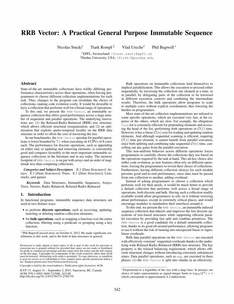
2.1 Radix-Balanced Tree StructureA Radix-Balanced tree is a shallow and complete (or perfect) m-arytree located only in the leaves. The nodes have a fixed branchingsize m, and are either internal nodes linking to sub-trees or leavescontaining elements. In practice the branching used is 32 [4, 37],but as we will later see, the node size can be any power of 2,allowing efficient radix-based implementations. Figure 1 shows

2 https://github.com/nicolasstucki/scala-rrb-vector3 Base structure for Relaxed-Radix-Balanced Vector.

0 1 … m-1

0 1 … m-1 0 1 … m-1

0 1 … m-1

0 1 … m-1

0 1 … m-1 0 1 … m-1 0 1 … m-1 0 1 … m-1

Figure 1. Radix-Balanced tree structure

this structure for m children on each node. Logically each nodeis a copy-on-write array that contains subtrees or elements.

Apart from the tree itself, a Vector keeps the tree height asa field, in order to improve performance. This height is upperbounded by logm(n−1)+1 for nodes of m branches. For example,if m is 32, the tree becomes quite shallow and the complexity totraverse it from root to leaf is considered as effectively constant4

when taking into account that the number of elements will neverbe larger than the maximum index representable with 32 bit signedintegers, which corresponds to a maximum height of 7 levels5.

Usually the number of elements in a Vector does not exactlymatch a full tree (mi for some i > 0). To mark the start and endof the elements in the tree, the vector keeps these indices as fields.All subtrees on the left and right that are outside of the filled indexrange are represented by empty references.

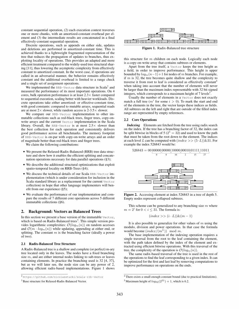
2.2 Core OperationsIndexing Elements are fetched from the tree using radix search

on the index. If the tree has a branching factor of 32, the index canbe split bitwise in blocks of 5 (25 = 32) and used to know the paththat must be taken from the root down to the element. The indicesat each level L can be computed with (index >> (5 ·L))&31. Forexample the index 526843 would be:

526843 = 00 000000

000000

1000016

000102

0111115

1101127

0 … 16 … 31

0 … 27 … 31

0 … 31

0 1 2 … 31

0 … 15 … 31

Figure 2. Accessing element at index 526843 in a tree of depth 5.Empty nodes represent collapsed subtrees.

This scheme can be generalized to any branching size m wherem = 2i for 0 < i ≤ 31. The formula is:

(index >> (i · L))&(m− 1)

It is also possible to generalize for other values of m using themodulo, division and power operations. In that case the formulawould become (index/(mL)) mod m.

The base implementation of the indexing operation requires asingle traversal from the root to the leaf containing the element,with the path taken defined by the index of the element and ex-tracted using efficient bitwise operations. With this traversal of thetree, the complexity of the operation is O(logm(n)).

The same radix-based traversal of the tree is used in the rest ofthe operations to find the leaf corresponding to a given index. It canbe optimized for the first and last leaf by removing computations toimprove performance on operations on the ends.

4 There exists a small enough constant bound (due to practical limitations).5 Maximum height of log32(231) + 1, which is 6.2.

343

1 type Node = Array[AnyRef]2 val Node = Array

1 val i = // bits in blocks of the index2 val mask = (1 << i) - 13 def get(index: Int): A = {4 def getRadix(idx: Int, nd: Node, level: Int): A = {5 if (depth == 0) nd(idx & mask)6 else {7 val indexInLevel = (idx >> (level * i)) & mask8 getRadix(idx, nd(indexInLevel), level-1)9 }

10 }11 getRadix(index, vectorRoot, vectorDepth)12 }

Updating Since the structure is immutable, the updatedoperation has to recreate the entire path from the root to the elementbeing updated. The leaf update creates a fresh copy of the leafarray with one updated element. Then, the parent of the leaf is alsoupdated with the reference to the new leaf, then the parent’s parent,and so on all the way up to the root.

1 def updated(index: Int, elem: A) = {2 def updatedNode(node: Node, level: Int): Node = {3 val indexInNode = // compute index4 val newNode = copy(node)5 if(level == 0) {6 newNode(indexInNode) = elem7 } else {8 newNode(indexInNode) =

updatedNode(node(indexInNode), level-1)9 }

10 newNode11 }12 new Vector(updatedNode(vectorRoot, vectorDepth),

...)13 }

Therefore the complexity of this operation is O(m · logm(n)),since it traverses and recreates O(logm(n)) nodes of size O(m).For example, if some leaf has all its elements updated from left toright, the branch will be copied as many times as there are updates.We will later explain how this can be optimized by allowing tran-sient states that avoid re-creating the path to the root tree node witheach update (described in §4).

Appending front and back The implementation of appendedfront/back has two cases, depending on the current state of theRadix-Balanced tree: If the first/last leaf is not full the element isinserted directly and all nodes of the first/last branch are copied.If the leaf is full we must find the lowest node in the last branchwhere there is still room left for a new branch. Then a new branchthat only contains the new element is appended to it.

In both cases the new vector object will have the start/end indexdecreased/increased by one. When the root is full, the depth of thevector will also increase by one.

1 val m = // branching factor2 def appended(elem: A, whr: Where): Vector[A] = {3 def appended(node: Node, level: Int) = {4 val indexInNode = // compute index based on

start/end index5 if (level == 1)6 copyAndUpdate(node, indexInNode, elem)7 else8 copyAndUpdate(node, indexInNode,9 appended(node(indexInNode), level-1))

10 }11 def newBranch(depth: Int): Node = {12 val newNode = Node.ofDim(m)13 val idx = whr match {14 case Frt => m-115 case Bck => 016 }

17 newNode(idx) =18 if (depth == 1) elem19 else newBranch(depth-1)20 newNode21 }22 if (needNewRoot()) {23 val newRoot = whr match {24 case Frt => Node(newBranch(depth), root)25 case Bck => Node(root, newBranch(depth))26 }27 new Vector(newRoot, depth+1, ...)28 } else {29 new Vector(appendedFront(root, depth), depth, ...)30 }31 }

In the code above, isTreeFull and needNewRoot are op-erations that compute the answer using efficient bitwise operationson the start/end index of the vector.

Since the algorithm traverses and creates new nodes from theroot to a leaf, the complexity of the operation is O(m · logm(n)).Like the updated operation, it can be optimized by keeping tran-sient states of the immutable vector (described in §4).

Splitting The core operations to remove elements in a Radix-Balanced tree are the take and drop operations. They are used toimplement many other operations such as splitAt, tail, initand others.

The take and drop operations are similar. The first step istraversing the tree down to the leaf where the cut will be done.Then the branch is copied and cleared on one side. The tree maybecome shallower during this operation, in which case some of thenodes on the top will be dropped instead of being copied. Finally,the start and end are adjusted according to the changes on the tree.

1 def take(index) = split(index, Right)2 def drop(index) = split(index, Left)3 def split(index: Int, removeSide: Side) = {4 def splitRec(node: Node, level: Int): (Node, Int) =

{5 val indexInNode = // compute index6 if (level == 0) {7 (copyAndSplitNode(node, indexInNode,

removeSide), 1)8 } else removeSide match {9 case Left if indexInNode == node.length - 1 =>

10 splitedRec(node(indexInNode), level - 1)11 case Right if indexInNode == 0 =>12 splitedRec(node(indexInNode), level - 1)13 case _ =>14 val newNode = copyAndSplitNode(node,

indexInNode, removeSide)15 val (newSubnode, depth) =

splitedRec(node(indexInNode), level-1)16 newNode(indexInNode) = newSubnode17 (newNode, level)18 }19 }20 val (newRoot, newDepth) = splitRec(vectorRoot,

vectorDepth)21 new Vector(newRoot, newDepth, ...)22 }

The computational complexity of any split operation is O(m ·logm(n)) due to the traversal and copying of nodes on the branchwhere the cut index is located. O(logm(n)) for the traversal ofthe branch and then O(m · logm(n2)) for the creation of the newbranch, where n2 is the size of the new vector (with 0 ≤ n2 < n).

3. Immutable Vectors as Relaxed Radix TreesRelaxed-Radix-Balanced vectors use a new tree structure that ex-tends the Radix-Balanced trees to allow fast concatenation of vec-tors without losing performance on other core operations [4]. Re-laxing the vector consists in using a slightly unbalanced extensionof the tree that combines balanced subparts. This vector still en-

344

sures the logm(n) bound on the height of the tree and on the oper-ations presented in the previous section.

3.1 Relaxed-Radix-Balanced Tree StructureThe basic difference in the structure is that in an Relaxed-Radix-Balanced (or RRB) tree, we allow nodes that contain subtrees thatare not completely full. As a consequence, the start and end indexare no longer required, as the branches on the ends can be truncated.The structure of the RRB trees does not ensure by itself that the treeheight is bounded by logm(n). This bound is maintained by eachoperation using an additional invariant on the tree balance. In ourcase the concatenation operation is the only one that can affect theinner structure (excluding ends) of the tree and as such it is the onlyone that needs to worry about this invariant.

Tree balance As the tree will not always be perfectly balanced,we define an additional invariant on the tree that will ensure anequivalent logarithmic bound on the height. We use the relationbetween the maximum and minimum branching factor mmax andmmin at each level. These give corresponding maximum heighthmax and least height hmin needed to represent a given number ofelements n. Then hmin = logmmax(n) and hmax = logmmin(n)or as hmin = 1

lg(mmax)·lg(n) and hmax = 1

lg(mmin)·lg(n). Trees

that are better balanced will have a height ratio, hr = lg(mmin)lg(mmax)

,that is closer to 1, perfect balance. In our tree we use mmax =mmin + 1 to make hr as close to 1 as possible. In practice (usingm = 32) in the worst case scenario there is an increase from around6.2 to 6.26 in the maximum possible height (i.e. 7 levels in bothcases).

Sizes metadata When one of these trees (or subtrees) isunbalanced, it is no longer possible to know the location of anindex just by applying radix manipulation on it. To avoid losingthe performance of traversing down the tree in such cases, eachunbalanced node will keep metadata on the sizes of its subtrees. Thesizes are kept in a separate6 copy-on-write array as accumulatedsizes. This way, they represent the location of the ranges of theindices in the current subtree. To avoid creating additional objectsin memory, these sizes are attached at the end of the node. To have ahomogeneous representation of nodes, the balanced subtrees havean empty reference attached at the end. For leaves, however, wemake an exception: since they will always be balanced, they onlycontain the data elements but not the size metadata.

0 1 … m-1 m

0 1 … m-1 0 1 … m-1

0 1 … m-1 m

0 1 … m-1 m

0 1 … m-1

0 1 … m-1

0 1 … m-1 0 1 … m-1 0 1 … m-1

Figure 3. Relaxed radix balanced tree structure

3.2 Relaxed Core OperationsAlgorithms for the relaxed version assume that the tree is unbal-anced and use a relaxed version of the code for Radix-Balancedtrees. But, as soon as a balanced subtree is encountered the moreefficient radix based algorithm is used. We also favor the creationof balanced trees/subtrees when possible to improve performanceon subsequent operations.

Indexing When the tree is relaxed it is not possible to com-pute the sub-indices directly from the index. By keeping the accu-mulated sizes in the node the computation of sub-indices becomestrivial. The sub-index is the same as the first index in the sizes array

6 To be able to share them across different vectors. This is a common casewhen using updated.

where index < sizes[subIndex]. The fastest way to find it is byusing binary search to reduce the search space and when it is smallenough to take advantage of cache lines and switch to linear search.

1 def getBranchIndex(sizes: Array[Int], indexInTree:Int): Int = {

2 var (lo, hi) = (0, sizes.length)3 while (linearThreshold < hi - lo) {4 val mid = (hi + lo) / 25 if (sizes(mid) <= indexInTree) lo = mid6 else hi = mid7 }8 while (sizes(lo) <= indexInTree) lo += 19 lo

10 }

Note that to traverse the tree down to the leaf where the indexis located, the sub-indices are computed from the sizes as longas the tree node is unbalanced. If the node is balanced, then themore efficient radix based method is used from there to the leaf,to avoid accessing the additional array in each level. In the worstcase the complexity of indexing will becomeO(log2(m)·logm(n))where log2(m) is a constant factor that is only added on unbalancednodes.1 def get(index: Int): A = {2 def getRadix(idx, Int, node: Node, depth: Int) = ...3 def get(idx: Int, node: Node, depth: Int) = {4 val sizes = // get sizes from node5 if(isUnbalanced(sizes)) {6 val branchIdx = getBranchIndex(sizes, idx)7 val subIdx = indexInTree-sizes(branchIdx)8 get(subIdx, node(branchIdx), depth-1)9 } else getRadix(idx, node, depth)

10 }11 get(index, root, depth)12 }

Updating and Appending For each one of these operations,the only fundamental difference with the Radix-Balanced tree isthat when a node of a branch is updated the sizes must be updatedwith it (if needed). In the case of updating, the structure does notchange and as such it always keeps the same sizes object reference.The traversal down the tree is done using the new abstraction usedin the relaxed version of indexing.

In the case of appending to the back, an updated unbalancednode must increment the accumulated size of its last subtree byone. When a new branch is appended, a new size is appended to thesizes. The newBranch operation is simplified by using truncatednodes and letting the node on which it gets appended handle anyindex shifting required.

1 def appended(elem: A, whr: Where): Vector[A] = {2 ...3 def newBranch(depth: Int): Node = {4 val newNode = Node.ofDim(1)5 newNode(0) = if (depth == 1) elem else

newBranch(depth-1)6 newNode7 }8 ...9 }

In the case of appending front, an updated node must incrementthe accumulated size of each subtrees by one. When a new branchis appended, a 1 is appended on the front of the sizes and all otheraccumulated sizes are incremented by one.

The complexity of these operations is still O(m · logm(n)),log2(m) · logm(n) for the traversal plus m · logm(n) for the branchupdate or creation.

Splitting While splitting, the traversal down the tree is doneusing the relaxed version of indexing. The splitting operation justtruncates the node on the left/right. In addition, when encounteringan unbalanced node, the sizes are truncated and adjusted. The

345

complexity of this operation is still O(m · logm(n)), log2(m) ·logm(n) for the traversal plus m · logm(n) for the branch update.

3.3 ConcatenationThe concatenation algorithm used on RRB-Vectors is a slightlymodified version of the one proposed in the RRB-Trees technicalreport [4]. This version favors nodes of size m over m− 1 makingthe trees more balanced. With this approach, we sacrifice a bit ofperformance for concatenations but we gain performance on allother operations: better balancing implies higher chance of usingfast radix operations on the trees.

From a high level, the algorithm merges the rightmost branchof the vector on the LHS with the leftmost branch of the vector onthe RHS. While merging the nodes, each of them is rebalanced inorder to ensure the O(logm(n)) bound on the height of the treeand avoid the degeneration of the structure. The RRB version ofconcatenation has a time complexity ofO(m2 · logm(n)) where mis constant.

1 def concatenate(left: Vector[A], right: Vector[A]) ={

2 val newTree = mergedTrees(left.root, right.root)3 val maxDepth = max(left.depth, right.depth)4 if (newTree.hasSingleBranch)5 new Vector(newTree.head, maxDepth)6 else7 new Vector(newTree, maxDepth+1)8 }9 def mergedTrees(left: Node, right: Node, depth: Int)

= {10 if (depth==1) {11 mergedLeaves(left, right)12 } else {13 val merged =14 if (depth==2) mergedLeaves(left.last,

right.first)15 else mergedTrees(left.last, right.first, depth-1)16 mergeRebalance(left.init, merged, right.tail)17 }18 }19 def mergedLeaves(left: Node, right: Node) = {20 // create a balanced new tree of height 221 // with all elements in the nodes22 }

The concatenation operation starts at the bottom of the branchesby merging the leaves into a balanced tree of height 2 usingmergedLeaves. Then, for each level on top of it, the newlycreated merged subtree and the remaining branches on that levelwill be merged and rebalanced into a new subtree. This new sub-tree always adds a new level to the tree, even though it might getdropped later. New sizes of nodes are computed each time a nodeis created based on sizes of children nodes.

Figure 4. Concatenation example: Rebalancing level 0

Figure 5. Concatenation example: Rebalancing level 1

The rebalancing algorithm has two proposed variants. The firstconsists of completely rebalancing the nodes on the two top levelsof the subtree. The second also rebalances the top two level ofthe subtree but it only rebalances the minimum amount of nodes

that ensures the logarithmic bound. The first one leaves the treebetter balanced, while the second is faster. As we aim to havegood performance on all operations we use the first variant7. Thefollowing snippet of code shows a high level implementation forthis first variant. Details for the second variant can be found in [4]in case that concatenation is prioritized over all other operations.

1 def mergeRebalance(left: Node, center: Node, right:Node) = {

2 // join all branches3 val merged = left ++ centre ++ right4 var newRoot = new ArrayBuilder5 var newSubtree = new ArrayBuilder6 var newNode = new ArrayBuilder7 def checkSubtree() = {8 if(newSubtree.length == m) {9 newRoot += computeSizes(newSubtree.result())

10 newSubtree.clear()11 }12 }13 for (subtree <- merged; node <-subtree) {14 if(newNode.length == m) {15 checkSubtree()16 newSubtree += computeSizes(newNode.result())17 newNode.clear()18 }19 newNode += node20 }21 checkSubtree()22 newSubtree += computeSizes(newNode.result())23 computeSizes(newRoot.result)24 }

Figures 4, 5, 6 and 7 show a concrete step by step (level bylevel) example of the concatenation of two vectors. In the example,some of the subtrees were collapsed. This is not only to make thediagrams fit, but also to expose only the nodes that are referencedduring the execution of the algorithm. Nodes with colors representnew nodes and changes, to help track them from figure to figure.

Figure 6. Concatenation example: Rebalancing level 2

Figure 7. Concatenation example: Rebalancing level 3

The concatenation algorithm chosen for the RRB Vector is theone that is slower but that is better at rebalancing. The reason be-hind this decision is that with better balanced trees all other oper-ations on the trees are more efficient. In fact, choosing the leastefficient option does not need to be seen as a reduction in per-formance, because the improvement is in relation to the Relaxed-Balanced tree concatenation of linear complexity. An interestingconsequence of this choice is that all trees (or subtrees) of size atmost m2 (the maximum size of a two level RRB tree) that werecreated by concatenation will be completely balanced.

It is important to have a smart rebalancing implementation, dueto the m2 elements that can possibly be accessed. The first crucialfactor is the speed of copying the nodes. With an implementationthat takes advantage of spatial locality by using arrays (§5.2), theamount of work required can be reduced to m fast node copies

7 Performance of operations using the second variant was analyzed in [37].

346

rather than m2 element copies. Another crucial but obvious imple-mentation detail is to never duplicate a node if it does not change.This requires a small amount of additional logic and comes with abenefit on memory used and in good cases can reduce the numberof node copies required, potentially reducing the effective work too(m ∗ logm(n)) if there is a good alignment.

When improving the vector on locality (§4), concatenating asmall vector using the concatenation algorithm is less efficient thanappending directly on the other tree. That case is identified by asimple bound on the lengths, and then all elements from the smallervector are appended to the larger one.

Other Operations Having efficient concatenation and spittingallows us to also implement several other operations that changethe structure of the tree. Some of there operations are: inserting anelement/vector in any position, deleting an element/subrange of thevector and patching/replacing part of the vector. The complexityof these operations are bounded by the complexity of the coreoperations used.

Parallelizing the Vector To parallelize operations we use thefork-join pool model from Java [18, 31]. In this model process-ing is achieved by splitting the work into smaller parts until theyare deemed small enough to ensure good parallelism. This can beachieved using the efficient splitting of the RRB-Tree. For certainoperations, like map, filter and reduce, the results obtained inparallel must be aggregated, such as concatenating the partial vec-tors produced by the parallel workers. The aggregation can oc-cur in several steps, where partial results from different workersare aggregated in parallel, recursively, until a single result is pro-duced. The overhead associated with the distribution of work isO(m2 · logm(n)).

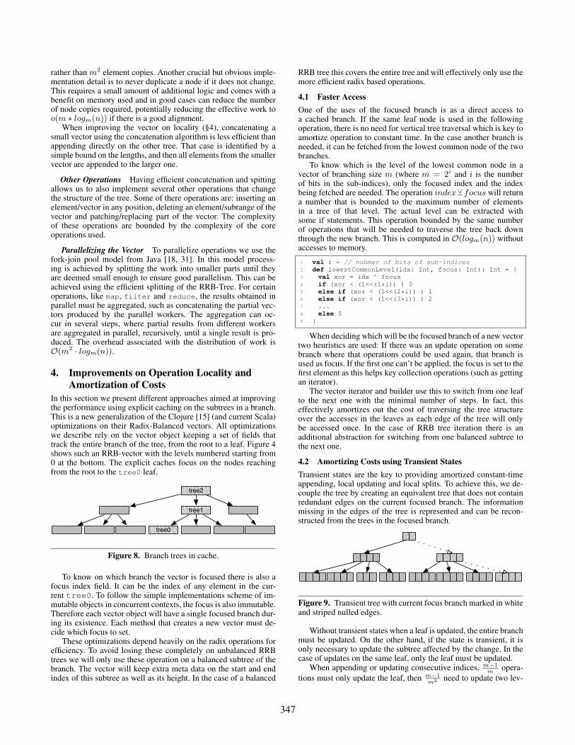
4. Improvements on Operation Locality andAmortization of Costs

In this section we present different approaches aimed at improvingthe performance using explicit caching on the subtrees in a branch.This is a new generalization of the Clojure [15] (and current Scala)optimizations on their Radix-Balanced vectors. All optimizationswe describe rely on the vector object keeping a set of fields thattrack the entire branch of the tree, from the root to a leaf. Figure 4shows such an RRB-vector with the levels numbered starting from0 at the bottom. The explicit caches focus on the nodes reachingfrom the root to the tree0 leaf.

tree0

tree2

tree1

Figure 8. Branch trees in cache.

To know on which branch the vector is focused there is also afocus index field. It can be the index of any element in the cur-rent tree0. To follow the simple implementations scheme of im-mutable objects in concurrent contexts, the focus is also immutable.Therefore each vector object will have a single focused branch dur-ing its existence. Each method that creates a new vector must de-cide which focus to set.

These optimizations depend heavily on the radix operations forefficiency. To avoid losing these completely on unbalanced RRBtrees we will only use these operation on a balanced subtree of thebranch. The vector will keep extra meta data on the start and endindex of this subtree as well as its height. In the case of a balanced

RRB tree this covers the entire tree and will effectively only use themore efficient radix based operations.

4.1 Faster AccessOne of the uses of the focused branch is as a direct access toa cached branch. If the same leaf node is used in the followingoperation, there is no need for vertical tree traversal which is key toamortize operation to constant time. In the case another branch isneeded, it can be fetched from the lowest common node of the twobranches.

To know which is the level of the lowest common node in avector of branching size m (where m = 2i and i is the numberof bits in the sub-indices), only the focused index and the indexbeing fetched are needed. The operation indexYfocus will returna number that is bounded to the maximum number of elementsin a tree of that level. The actual level can be extracted withsome if statements. This operation bounded by the same numberof operations that will be needed to traverse the tree back downthrough the new branch. This is computed in O(logm(n)) withoutaccesses to memory.

1 val i = // nubmer of bits of sub-indices2 def lowestCommonLevel(idx: Int, focus: Int): Int = {3 val xor = idx ^ focus4 if (xor < (1<<(1*i)) ) 05 else if (xor < (1<<(2*i)) ) 16 else if (xor < (1<<(3*i)) ) 27 ...8 else 59 }

When deciding which will be the focused branch of a new vectortwo heuristics are used: If there was an update operation on somebranch where that operations could be used again, that branch isused as focus. If the first one can’t be applied, the focus is set to thefirst element as this helps key collection operations (such as gettingan iterator).

The vector iterator and builder use this to switch from one leafto the next one with the minimal number of steps. In fact, thiseffectively amortizes out the cost of traversing the tree structureover the accesses in the leaves as each edge of the tree will onlybe accessed once. In the case of RRB tree iteration there is anadditional abstraction for switching from one balanced subtree tothe next one.

4.2 Amortizing Costs using Transient StatesTransient states are the key to providing amortized constant-timeappending, local updating and local splits. To achieve this, we de-couple the tree by creating an equivalent tree that does not containredundant edges on the current focused branch. The informationmissing in the edges of the tree is represented and can be recon-structed from the trees in the focused branch.

Figure 9. Transient tree with current focus branch marked in whiteand striped nulled edges.

Without transient states when a leaf is updated, the entire branchmust be updated. On the other hand, if the state is transient, it isonly necessary to update the subtree affected by the change. In thecase of updates on the same leaf, only the leaf must be updated.

When appending or updating consecutive indices, m−1m

opera-tions must only update the leaf, then m−1

m2 need to update two lev-

347

els of the tree and so on. These operations will thus be amortizedto constant time if they are executed in succession. This is due tothe bound given by average number of node update per operation:∑∞

k=1k·(m−1)

mk = mm−1

.There is a cost associated to the transformation from canonical

to transient state and back. This cost is equivalent to one update ofthe focused branch. The transient state operations only start payingoff after 3 consecutive operations. With 2 consecutive operationsthey are matched and with 1 there is a loss in performance.

Canonicalization The transient state aims to improve perfor-mance of some operations by amortizing costs. But, the transientstate is not ideal for performance of other operations. For examplean indexing operation on an unbalanced vector may lack the sizeinformation it requires to efficiently access certain indices. And aniterator relies on a canonical tree for performance. It is possible toimplement these operations on a transient state, but this involvesboth code duplication and additional overhead on each call.

The solution we used involves converting the transient represen-tation to a canonical one. This conversion, called canonicalization,is applied when an operation that requires the cannonical form iscalled on an instance of the immutable vector. The mutation of thevector is not visible from the outside and only happens at most once(Figure 10). This transformation only affects the nodes that are onthe focused branch, as it copies each one (except the leaf) and linksthe trees. If the node is unbalanced, the size of the subtree in focusis inserted. This transformation could be seen as a lazy initializationof the current branch.

Figure 10. Objects states and effect of operations.

Vector objects can only be in the transient state if they werecreated this way. For example, the appending operations will createa new object that is in transient state and focused on the last/firstbranch. If the source object was not focusing the last branch, thenit is canonicalized (if needed) before change of branch operation.Vectors of depth 1 are special cases, they are always in canonicalform and their operations are equivalent to those in transient form.

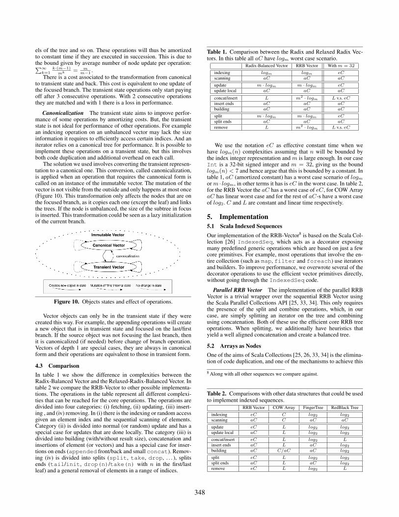
4.3 ComparisonIn table 1 we show the difference in complexities between theRadix-Balanced Vector and the Relaxed-Radix-Balanced Vector. Intable 2 we compare the RRB-Vector to other possible implementa-tions. The operations in the table represent all different complexi-ties that can be reached for the core operations. The operations aredivided into four categories: (i) fetching, (ii) updating, (iii) insert-ing , and (iv) removing. In (i) there is the indexing or random accessgiven an element index and the sequential scanning of elements.Category (ii) is divided into normal (or random) update and has aspecial case for updates that are done locally. The category (iii) isdivided into building (with/without result size), concatenation andinsertions of element (or vectors) and has a special case for inser-tions on ends (appended front/back and small concat). Remov-ing (iv) is divided into splits (split, take, drop, . . . ), splitsends (tail/init, drop(n)/take(n) with n in the first/lastleaf) and a general removal of elements in a range of indices.

Table 1. Comparison between the Radix and Relaxed Radix Vec-tors. In this table all aC have logm worst case scenario.

Radix-Balanced Vector RRB Vector With m = 32

indexing logm logm eCscanning aC aC aC

update m · logm m · logm eCupdate local aC aC aC

concat/insert L m2 · logm L v.s. eCinsert ends aC aC aCbuilding aC aC aC

split m · logm m · logm eCsplit ends aC aC aC

remove L m2 · logm L v.s. eC

We use the notation eC as effective constant time when wehave logm(n) complexities assuming that n will be bounded bythe index integer representation and m is large enough. In our caseInt is a 32-bit signed integer and m = 32, giving us the boundlogm(n) < 7 and hence argue that this is bounded by a constant. Intable 1, aC (amortized constant) has a worst case scenario of logmor m · logm, in other terms it has is eC in the worst case. In table 2,for the RRB Vector the aC has a worst case of eC, for COW ArrayaC has linear worst case and for the rest of aC-s have a worst caseof log2. C and L are constant and linear time respectively.

5. Implementation5.1 Scala Indexed SequencesOur implementation of the RRB-Vector8 is based on the Scala Col-lection [26] IndexedSeq, which acts as a decorator exposingmany predefined generic operations which are based on just a fewcore primitives. For example, most operations that involve the en-tire collection (such as map, filter and foreach) use iteratorsand builders. To improve performance, we overwrote several of thedecorator operations to use the efficient vector primitives directly,without going through the IndexedSeq code.

Parallel RRB Vector The implementation of the parallel RRBVector is a trivial wrapper over the sequential RRB Vector usingthe Scala Parallel Collections API [25, 33, 34]. This only requiresthe presence of the split and combine operations, which, in ourcase, are simply splitting an iterator on the tree and combiningusing concatenation. Both of these use the efficient core RRB treeoperations. When splitting, we additionally have heuristics thatyield a well aligned concatenation and create a balanced tree.

5.2 Arrays as NodesOne of the aims of Scala Collections [25, 26, 33, 34] is the elimina-tion of code duplication, and one of the mechanisms to achieve this

8 Along with all other sequences we compare against.

Table 2. Comparisons with other data structures that could be usedto implement indexed sequences.

RRB Vector COW Array FingerTree RedBlack Tree

indexing eC C log2 log2scanning aC C aC aC

update eC L log2 log2update local aC L log2 log2

concat/insert eC L log2 Linsert ends aC L aC log2building aC C/aC aC log2

split eC L log2 log2split ends aC L aC log2remove eC L log2 L

348

is the use of generic types [9, 22]. But this also has a drawback: theneed to box primitive values in order for them to be stored in thecollection. We implemented all our sequences in this context.

All nodes are stored in arrays of type Array[AnyRef], sincethis allows us to quickly access elements (which are boxed any-way due to generics9) without dispatching on the primitive arraytype. A welcome side effect of this decision is that elements arealready boxed when they are passed to the Vector, thus accessingand storing them does not incur any intermediate boxing/unbox-ing operations, which would add overhead. However, it is knownthat using the boxed representation for primitive types is inefficientwhen operating on the values themselves, so the sizes of unbal-anced nodes are stored in Array[Int] objects, guaranteeing themost compact and efficient data representation.

Most of the memory used in the vector data structure will becomposed of arrays. There are three key operations used on thesearrays: creation, update and access. Since the arrays are used withcopy-on-write semantics, actual update operations are only allowedwhen the array is initialized. This also implies that each time thereis a modification on some part of an array, a new array must becreated and the old elements must be copied.

The size of the array will affect the performance of the vector.With larger arrays in the nodes the access times will be reducedbecause the depth of the tree will decrease. But, on the otherhand, increasing the size of the arrays will slow down the updateoperations, as they have to copy the entire array to execute theelement update, due to the copy-on-write semantics.

For an individual reference to an RRB-Vector of size n andbranching of m, the memory usage will composed by the arrayslocated in the leaves10 and the ones that form the tree structure.In our case we save references and hence we need d n

me arrays

of m references11. The structure requrires at least the referencesto the child nodes and in the worst case scenario an additionalinteger the size of each child. Going up level by level, the referencecount decreases by a factor of m and hence the total is boundedby

∑logm(n)k=2 d n

mk e <∑∞

k=2dn

mk e ≤ n+mm·(m−1)

refrences. For thesizes of the nodes, given our choice of rebalancing algorithm, theywill only appear on nodes that are of height 3 or larger and hencethe sizes will be bounded by

∑logm(n)k=3 d n

mk e <∑∞

k=3dn

mk e ≤n+m

m2·(m−1)integers.

5.3 Running on a JVMIn practice, Scala compiles to Java bytecode and executes on a JavaVirtual Machine (JVM), where we used the Oracle Java SE dis-tribution [29] as a reference. This imposes additional characteris-tics of performance that can’t be evaluated on the algorithmic levelalone, and ask for a more nuanced discussion.

One of the JVM components that directly affects vectors is thegarbage collector (or GC). Vector operations tend to create a largenumber of Array objects, some of which are only necessary for ashort time. These objects will use up memory and thus degradeoverall performance as the GC is invoked more often. For thisreason our code is optimized to avoid the redundant creation ofintermediary objects, delaying the GC cycles and thus improvingperformance.

Instead of directly compiling bytecode to native code, the JVMuses a just in time compilation (JIT) mechanism in order to take ad-vantage of run-time profiling information. At first it runs the com-piled bytecode inside an interpreter and collects execution statis-tics (profiles). Later, once a method has executed enough times, it

9 A limitation that could be circumvented by Miniboxing [40].10 Note that the memory used in the leaves is equivalent to the memory usedfor an array that contains all the elements.11 It could be any kind of data.

compiles it using the statistics to guide optimizations. The Vectorcode tries to gain performance by aligning with the JIT heuristicsand hence taking advantage of its optimizations. The most impor-tant such optimization is inlining, which eliminates the overhead ofcalling a method and, furthermore, enables other optimizations toimprove the inlined code. Critical parts of the Vector code are care-fully designed to to match the heuristics of the JVM. In particular,a heuristic that arose commonly is that only methods of size lessthan 35 bytes are inlined, which meant we had to split the code intoseveral methods to stay below this threshold.

6. Evaluation6.1 MethodologyScalaMeter [30] is used to measure performance of operations ondifferent implementations of indexed sequences.

To have reproducible results with low error margins, ScalaMe-ter was configured on a per benchmark basis. Each test is run on32 different JVM instances to average out badly allocated VMs.On each JVM, 32 measurements were taken and they were filteredusing outlier elimination to remove those runs that where excep-tionally different. This could happen if a more thorough garbagecollection cycle occurs in a particular run, due to JIT compilationor if the operating system switches to a more important task dur-ing the benchmark process [12]. Before taking measurements, theJVM is warmed up by running the benchmark code several times,without taking the measurements into account. This allows us tomeasure the time after the JIT compilation has occurred, when thesystem is in a steady state.

There are three main directions in the performance compar-isons. The first compares the Radix-Balanced vectors with well-balanced RRB Vectors, with the goal of having an equivalent per-formance, even if the RRB Vectors have an inherent additionaloverhead. The second axis shows the effects of unbalanced nodeson RRB-Tree. For this we compare the same perfect balanced vec-tor with an extremely unbalanced vector. The later vector is gener-ated by concatenating pseudo-random small vectors together. Theamount of unbalanced nodes is in part affected by the size of thevector. The third axis is the comparison between vectors in generaland other well known functional and/or immutable data structuresused to implement sequences. We used a copy-on-write (COW) ar-rays, finger trees [16] (FingerTreeSeq12) and red black trees [13](RedBlackSeq13).

6.2 ResultsFor the results of this sections, benchmarks where executed on aJava HotSpot(TM) 64-Bit Server VM on a machine with an Intel(R)Core(TM) i7-4770 CPU @ 3.40GHz with 32GiB on RAM. Eachbenchmarking VM instance was setup with 16GiB of heap memory.The parallel vector split-combine was executed on a machine with4 Intel(R) Xeon(R) Processors, of type E5-4640 @ 2.40GHz with128GiB on RAM.

Iterating The benchmark in Figure 11 shows the time it takesto scan the whole sequence using a specialized iterator. Unsurpris-ingly, the results show that the best option is the array. But the vec-tor is only 1-2× slower, closer to 1× in the most common cases.It is also possible to see that vectors are 7-15× faster than otherdeeper trees, mainly due to the reduction in indirections and in-creased locality.

Building The benchmark in Figure 12 shows the time it takesto build a sequence using a specialized builder. In general, the

12 Adapted version of https://github.com/Sciss/FingerTree whereabstractions that did not involve sequences where removed.13 Adaptation of the standard Scala Collections RedBlackTree where keysare used as indices.

349

Figure 11. Iterating through the sequence

Figure 12. Building a sequence.

builder for these sequences does not know the size of the resultingsequence. In the case of array builder there is the possibility ofgiving it a hint of the result size (Hinted in the benchmarks). Inthis case the vector wins against all other implementations. It isfaster than other trees because they require re-balancing during thebuilding, whereas the vector behaves more like an array buildingby allocating chunks of memory and filling them. Array buildingrequires resizing of the array whenever it is filled or the result isreturned, which implies a copy of the whole array. By contrast, thevector only requires a copy of the last branch when returned. This isthe main reason the vector is able to outperform the array buildingprocess. Also, the standard array builder uses the hint as such andtherefore still requires some copies of the array.

Indexing Figure 13 shows the time taken to access 10k ele-ments in consecutive indices while Figure 14 shows the same forrandomly chosen indices. From the algorithmic point of view theyare exactly the same, the difference is in how the memory is kept inthe processor caches. It shows that in either cases the vector accessbehaves effectively as constant time like the array, where the fingertrees and red black trees degenerate with randomness. A vector ofdepth 3 is 2-3.5× slower than the array, the cost of accessing thearrays in the 3 levels of the branches.

Figure 13. Accessing 10k consecutive indices

Figure 14. Accessing 10k random indices

Updating Figure 15 shows the time taken to update 10kelements in consecutive indices and Figure 16 shows the same forrandomly chosen indices. In this case the array is clearly the worstoption because it creates a new version and copies the contents witheach update. The vector behaves effectively as having constant timewhile taking advantage of locality and degenerates slightly withrandomness. The vector is 4.3× faster on local updates and 1-2.3×faster on random updates than the red black tree.

Concatenating Figures 17 and 18 show the time it takes toconcatenate two sequences (two points of view of the same 3Dplot). The two axes on the bottom represent the sizes of the LHS(left hand side) and RHS (right hand side) of the concatenationoperation. It can be seen that the RRB Vector and finger trees arealmost equivalent in performance (bottom planes). The array up toa result size of 4096 is able to concatenate faster thanks to locality,but then grows linearly with the result size (middle plane). Thevector without efficient concatenation (on Radix-Balanced trees)behaves just like the array but with worse constant factors (topplane). The red black tree was omitted from this graph due itsinefficient concatenation operation.

Appending Figures 19 and 20 show the time it takes toappend 256 elements on by one. In the first case we append them

350

Figure 15. Updating on 10k consecutive indices

Figure 16. Updating on 10k random indices

to the front and in the second to the back of the sequence. Thelarge number of elements was chosen in order show the amortizedtime of the operation on the vectors. In this case the array isclearly the worst option because it creates a new version and copiesthe contents with each append. The vector is around 2.5× slowerthan the finger trees, a structure that specifically focuses on theseoperations. The vector can be 1-2× faster than a red black tree.

Splitting Figures 21 and 22 show the time it takes to split asequence on the left and on the right. We fixed the cut point tothe middle of the sequence to be able to compare the time it takesto take or drop the same number of elements. It can be seen thatsplitting a vector is more efficient than other structures. Even more,the vector behaves with an effectively constant time.

Parallel Vector Split-combine Overhead The benchmarks inFigure 23 and 24 show the amount of overhead associated with theparallelization of the vector with and without efficient concatena-tion. They show the typical overhead of a parallel map, filter orother similar operations that create a new version of the sequence.The benchmark computes a map operation using the identity func-tion, such that the execution time is dominated by the time it takesto split and combine the sequence rather than the function compu-tations. As a base for comparison we used the sequential map on

Figure 17. Concatenating two sequences (point of view 1). RRBVector and Finger Tree are the planes at the bottom, COW Array isthe plane in the middle and Vector is the plane on the top.

Figure 18. Concatenating two sequences (point of view 2). Moreinformationg on the first point of view on figure 17.

both versions, where the results are identical. Then we parallelizedit on fork-join thread pools of 1, 2, 4, 8, 16, 32 and 64 thread on a 64threaded (32 cores) machine. Without concatenation, there is a lossof performance on when passing from sequential to parallel and al-though the performance increases with the addition of threads, evenwith 64 threads it’s only slightly better than the sequential version.By contrast, with our new vector, the gain in performance startswith one thread in the pool (dedicated thread) and then increases.Giving a 1.55× increase with 2 threads, 2.46× for 4 thread, 3.52×for 8 thread, 4.60× for 16 thread, 5.52× for 32 thread (core limit)and 7.18× for 64 thread (hardware thread limit).

Memory Overhead Figure 25 shows the memory overhead ofthe data structures used in the benchmarks. This overhead is theadditional space used in relation to the COW Array. The overheadof a vector is 17.5× smaller than the finger tree and 40× smallerthan the red black trees.

7. Related WorkRelated data structures There is a strong relation between

RRB Trees and various data structures in the literature. Patriciatries [24] are one of the earliest documented uses of radix trees, per-forming lookups and updates one bit or character at a time. Widerradix trees were used to build space efficient sparse arrays, ArrayMapped Tries (AMT) [1], and on top of that Hash Array MappedTries (HAMT) [2], which have been popularized and adapted to an

351

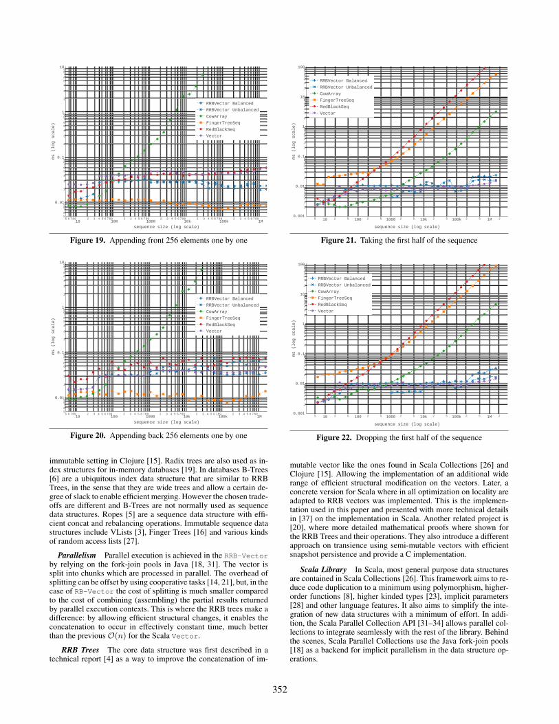
Figure 19. Appending front 256 elements one by one

Figure 20. Appending back 256 elements one by one

immutable setting in Clojure [15]. Radix trees are also used as in-dex structures for in-memory databases [19]. In databases B-Trees[6] are a ubiquitous index data structure that are similar to RRBTrees, in the sense that they are wide trees and allow a certain de-gree of slack to enable efficient merging. However the chosen trade-offs are different and B-Trees are not normally used as sequencedata structures. Ropes [5] are a sequence data structure with effi-cient concat and rebalancing operations. Immutable sequence datastructures include VLists [3], Finger Trees [16] and various kindsof random access lists [27].

Parallelism Parallel execution is achieved in the RRB-Vectorby relying on the fork-join pools in Java [18, 31]. The vector issplit into chunks which are processed in parallel. The overhead ofsplitting can be offset by using cooperative tasks [14, 21], but, in thecase of RB-Vector the cost of splitting is much smaller comparedto the cost of combining (assembling) the partial results returnedby parallel execution contexts. This is where the RRB trees make adifference: by allowing efficient structural changes, it enables theconcatenation to occur in effectively constant time, much betterthan the previous O(n) for the Scala Vector.

RRB Trees The core data structure was first described in atechnical report [4] as a way to improve the concatenation of im-

Figure 21. Taking the first half of the sequence

Figure 22. Dropping the first half of the sequence

mutable vector like the ones found in Scala Collections [26] andClojure [15]. Allowing the implementation of an additional widerange of efficient structural modification on the vectors. Later, aconcrete version for Scala where in all optimization on locality areadapted to RRB vectors was implemented. This is the implemen-tation used in this paper and presented with more technical detailsin [37] on the implementation in Scala. Another related project is[20], where more detailed mathematical proofs where shown forthe RRB Trees and their operations. They also introduce a differentapproach on transience using semi-mutable vectors with efficientsnapshot persistence and provide a C implementation.

Scala Library In Scala, most general purpose data structuresare contained in Scala Collections [26]. This framework aims to re-duce code duplication to a minimum using polymorphism, higher-order functions [8], higher kinded types [23], implicit parameters[28] and other language features. It also aims to simplify the inte-gration of new data structures with a minimum of effort. In addi-tion, the Scala Parallel Collection API [31–34] allows parallel col-lections to integrate seamlessly with the rest of the library. Behindthe scenes, Scala Parallel Collections use the Java fork-join pools[18] as a backend for implicit parallelism in the data structure op-erations.

352

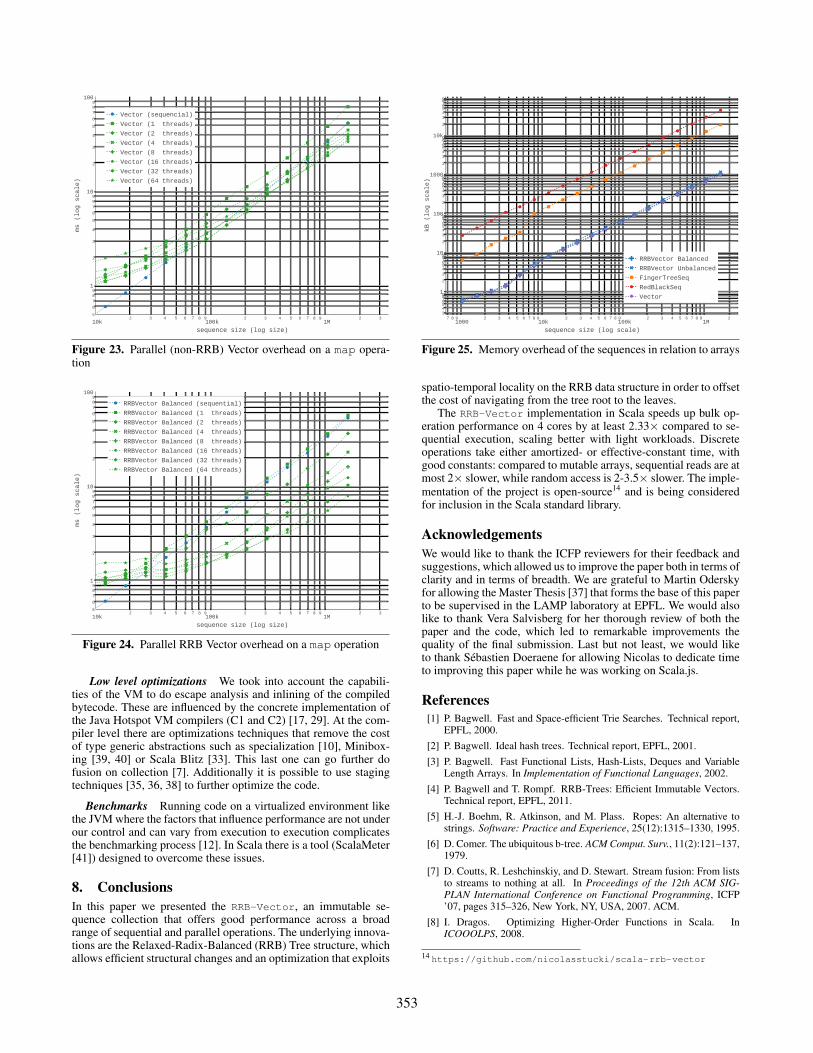
Figure 23. Parallel (non-RRB) Vector overhead on a map opera-tion

Figure 24. Parallel RRB Vector overhead on a map operation

Low level optimizations We took into account the capabili-ties of the VM to do escape analysis and inlining of the compiledbytecode. These are influenced by the concrete implementation ofthe Java Hotspot VM compilers (C1 and C2) [17, 29]. At the com-piler level there are optimizations techniques that remove the costof type generic abstractions such as specialization [10], Minibox-ing [39, 40] or Scala Blitz [33]. This last one can go further dofusion on collection [7]. Additionally it is possible to use stagingtechniques [35, 36, 38] to further optimize the code.

Benchmarks Running code on a virtualized environment likethe JVM where the factors that influence performance are not underour control and can vary from execution to execution complicatesthe benchmarking process [12]. In Scala there is a tool (ScalaMeter[41]) designed to overcome these issues.

8. ConclusionsIn this paper we presented the RRB-Vector, an immutable se-quence collection that offers good performance across a broadrange of sequential and parallel operations. The underlying innova-tions are the Relaxed-Radix-Balanced (RRB) Tree structure, whichallows efficient structural changes and an optimization that exploits

Figure 25. Memory overhead of the sequences in relation to arrays

spatio-temporal locality on the RRB data structure in order to offsetthe cost of navigating from the tree root to the leaves.

The RRB-Vector implementation in Scala speeds up bulk op-eration performance on 4 cores by at least 2.33× compared to se-quential execution, scaling better with light workloads. Discreteoperations take either amortized- or effective-constant time, withgood constants: compared to mutable arrays, sequential reads are atmost 2× slower, while random access is 2-3.5× slower. The imple-mentation of the project is open-source14 and is being consideredfor inclusion in the Scala standard library.

AcknowledgementsWe would like to thank the ICFP reviewers for their feedback andsuggestions, which allowed us to improve the paper both in terms ofclarity and in terms of breadth. We are grateful to Martin Oderskyfor allowing the Master Thesis [37] that forms the base of this paperto be supervised in the LAMP laboratory at EPFL. We would alsolike to thank Vera Salvisberg for her thorough review of both thepaper and the code, which led to remarkable improvements thequality of the final submission. Last but not least, we would liketo thank Sébastien Doeraene for allowing Nicolas to dedicate timeto improving this paper while he was working on Scala.js.

References[1] P. Bagwell. Fast and Space-efficient Trie Searches. Technical report,

EPFL, 2000.[2] P. Bagwell. Ideal hash trees. Technical report, EPFL, 2001.[3] P. Bagwell. Fast Functional Lists, Hash-Lists, Deques and Variable

Length Arrays. In Implementation of Functional Languages, 2002.[4] P. Bagwell and T. Rompf. RRB-Trees: Efficient Immutable Vectors.

Technical report, EPFL, 2011.[5] H.-J. Boehm, R. Atkinson, and M. Plass. Ropes: An alternative to

strings. Software: Practice and Experience, 25(12):1315–1330, 1995.[6] D. Comer. The ubiquitous b-tree. ACM Comput. Surv., 11(2):121–137,

1979.[7] D. Coutts, R. Leshchinskiy, and D. Stewart. Stream fusion: From lists

to streams to nothing at all. In Proceedings of the 12th ACM SIG-PLAN International Conference on Functional Programming, ICFP’07, pages 315–326, New York, NY, USA, 2007. ACM.

[8] I. Dragos. Optimizing Higher-Order Functions in Scala. InICOOOLPS, 2008.

14 https://github.com/nicolasstucki/scala-rrb-vector

353

[9] I. Dragos. Compiling Scala for Performance. PhD thesis, IC, 2010.[10] I. Dragos and M. Odersky. Compiling Generics through User-directed

Type Specialization. In ICOO0LPS ’09. ACM, 2009.[11] J. R. Driscoll, N. Sarnak, D. D. Sleator, and R. E. Tarjan. Making data

structures persistent. J. Comput. Syst. Sci., 38(1):86–124, Feb. 1989.[12] A. Georges, D. Buytaert, and L. Eeckhout. Statistically rigorous java

performance evaluation. In Proceedings of the 22Nd Annual ACMSIGPLAN Conference on Object-oriented Programming Systems andApplications, OOPSLA ’07, pages 57–76, New York, NY, USA, 2007.ACM.

[13] S. Hanke. The Performance of Concurrent Red-Black Tree Algo-rithms. In J. Vitter and C. Zaroliagis, editors, Algorithm Engineering,volume 1668 of Lecture Notes in Computer Science. Springer BerlinHeidelberg, 1999.

[14] M. Herlihy and N. Shavit. The Art of Multiprocessor Programming.Apr. 2008.

[15] R. Hickey. The Clojure programming language, 2006.[16] R. Hinze and R. Paterson. Finger Trees: A Simple General-purpose

Data Structure. J. Funct. Program., 16(2), 2006.[17] T. Kotzmann, C. Wimmer, H. Mössenböck, T. Rodriguez, K. Russell,

and D. Cox. Design of the Java HotSpot&Trade; Client Compiler forJava 6. ACM Trans. Archit. Code Optim., 5(1), May 2008.

[18] D. Lea. A Java Fork/Join Framework. In Proceedings of the ACM2000 Conference on Java Grande, JAVA ’00, New York, NY, USA,2000. ACM.

[19] V. Leis, A. Kemper, and T. Neumann. The adaptive radix tree: Artfulindexing for main-memory databases. In C. S. Jensen, C. M. Jermaine,and X. Zhou, editors, 29th IEEE International Conference on DataEngineering, ICDE 2013, Brisbane, Australia, April 8-12, 2013, pages38–49. IEEE Computer Society, 2013.

[20] J. N. L’orange. Improving RRB-Tree Performance through Tran-sience. Master’s thesis, Norwegian University of Science and Tech-nology, June 2014.

[21] Moir and Shavit. Concurrent data structures. In Mehta and Sahni,editors, Handbook of Data Structures and Applications, Chapman &Hall/CRC. 2005.

[22] A. Moors. Type Constructor Polymorphism for Scala: Theory andPractice (Type constructor polymorfisme voor Scala: theorie en prak-tijk). PhD thesis, Informatics Section, Department of Computer Sci-ence, Faculty of Engineering Science, May 2009. Joosen, Wouter andPiessens, Frank (supervisors).

[23] A. Moors, F. Piessens, and M. Odersky. Generics of a Higher Kind.Acm Sigplan Notices, 43, 2008.

[24] D. R. Morrison. PATRICIA-practical algorithm to retrieve informationcoded in alphanumeric. J. ACM, 15(4):514–534, Oct. 1968.

[25] M. Odersky. Future-Proofing Collections: From Mutable to Persistentto Parallel. In Compiler Construction, volume 6601 of Lecture Notesin Computer Science. Springer-Verlag New York, Ms Ingrid Cunning-ham, 175 Fifth Ave, New York, Ny 10010 Usa, 2011.

[26] M. Odersky and A. Moors. Fighting bit Rot with Types (ExperienceReport: Scala Collections). In R. Kannan and K. N. Kumar, edi-tors, IARCS Annual Conference on Foundations of Software Technol-ogy and Theoretical Computer Science, volume 4 of Leibniz Interna-tional Proceedings in Informatics (LIPIcs), Dagstuhl, Germany, 2009.Schloss Dagstuhl–Leibniz-Zentrum fuer Informatik.

[27] C. Okasaki. Purely Functional Data Structures. Cambridge UniversityPress, New York, NY, USA, 1998.

[28] B. C. d. S. Oliveira, A. Moors, and M. Odersky. Type Classes asObjects and Implicits. In OOPSLA ’10. ACM, 2010.

[29] M. Paleczny, C. Vick, and C. Click. The java hotspottm server com-piler. In Proceedings of the 2001 Symposium on JavaTM VirtualMachine Research and Technology Symposium - Volume 1, JVM’01,pages 1–1, Berkeley, CA, USA, 2001. USENIX Association.

[30] A. Prokopec. ScalaMeter. https://scalameter.github.io/.

[31] A. Prokopec. Data Structures and Algorithms for Data-Parallel Com-puting in a Managed Runtime. PhD thesis, IC, Lausanne, 2014.

[32] A. Prokopec and M. Odersky. Near optimal work-stealing tree sched-uler for highly irregular data-parallel workloads. In Languages andCompilers for Parallel Computing, Lecture Notes in Computer Sci-ence, pages 55–86. Springer International Publishing, 2014.

[33] A. Prokopec, D. Petrashko, and M. Odersky. Efficient Lock-FreeWork-stealing Iterators for Data-Parallel Collections. 2015.

[34] A. Prokopec, T. Rompf, P. Bagwell, and M. Odersky. On a genericparallel collection framework, 2011.

[35] T. Rompf and M. Odersky. Lightweight Modular Staging: A Prag-matic Approach to Runtime Code Generation and Compiled DSLs.Communications Of The Acm, 55, 2012.

[36] T. Rompf, A. K. Sujeeth, K. J. Brown, H. Lee, H. Chafi, and K. Oluko-tun. Surgical precision JIT compilers. In M. F. P. O’Boyle and K. Pin-gali, editors, ACM SIGPLAN Conference on Programming LanguageDesign and Implementation, PLDI ’14, Edinburgh, United Kingdom -June 09 - 11, 2014, page 8. ACM, 2014.

[37] N. Stucki. Turning Relaxed Radix Balanced Vector from Theory intoPractice for scala collections. Master’s thesis, EPFL, 2015.

[38] W. Taha and T. Sheard. MetaML and Multi-Stage Programming withExplicit Annotations. In Theoretical Computer Science. ACM Press,1999.

[39] V. Ureche, E. Burmako, and M. Odersky. Late data layout: Unifyingdata representation transformations. In Proceedings of the 2014 ACMInternational Conference on Object Oriented Programming SystemsLanguages &#38; Applications, OOPSLA ’14, pages 397–416, NewYork, NY, USA, 2014. ACM.

[40] V. Ureche, C. Talau, and M. Odersky. Miniboxing: Improving theSpeed to Code Size Tradeoff in Parametric Polymorphism Transla-tions. In OOPSLA’13, OOPSLA ’13, pages 73–92, New York, NY,USA, 2013. ACM.

[41] B. Venner, G. Berger, and C. C. Seng. Scalatest. http://www.scalatest.org/.

354