Routing protocols for interconnecting cellular and ad...
90
UNIVERSIT ´ E LIBRE DE BRUXELLES Facult´ e des Sciences D´ epartement d’Informatique Routing protocols for interconnecting cellular and ad-hoc networks M´ emoire pr´ esent´ e en vue de l’obtention du grade de Licenci´ e en Informatique Bayani Carbone Ann´ ee acad´ emique 2005–2006
Transcript of Routing protocols for interconnecting cellular and ad...
UNIVERSITE LIBRE DE BRUXELLESFaculte des SciencesDepartement d’Informatique
Routing protocols forinterconnecting cellular and ad-hoc
networks
Memoire presente en vue de l’obtentiondu grade de Licencie en Informatique
Bayani CarboneAnnee academique 2005–2006
Abstract
This study presents an original routing protocol for interconnecting andextending cellular networks, in particular UMTS networks, with Ad-Hocnetworks. This new protocol GWAODV 1 is based on already establishedAd-Hoc routing protocols: AODV[1] and ABR[2]. Simulations were runusing the NS-2[3] simulator to analyze the protocol’s performance in termsof end-to-end delay, packet delivery fraction and routing overhead.
1Gateway Ad-hoc On Demand Distance Vector
2

Acknowledgments
Above all, I would like to thank my parents and my girlfriend, without whomI would never have been able to finish this work. They have supported mesince day one and I am very grateful to have them in my life.
I would also like to thank my family and friends for their never endingsupport and their precious advises.
Of course, none of this would have been possible without Mr J-M. Dricot,Professor G. Bocq and Professor R. Devillers who found this subject for meand followed me every step of the way. For this I thank them and it hasbeen a pleasure working with them.
3

Contents
Abstract 2
Acknowledgments 3
1 Introduction 9
I State Of The Art 11
2 Cellular Networks 122.1 Introduction . . . . . . . . . . . . . . . . . . . . . . . . . . . . 122.2 UMTS services . . . . . . . . . . . . . . . . . . . . . . . . . . 132.3 UMTS Architecture . . . . . . . . . . . . . . . . . . . . . . . 13
2.3.1 Core Network . . . . . . . . . . . . . . . . . . . . . . . 152.3.2 UMTS Terrestrial Radio Access Network . . . . . . . 152.3.3 User Equipment . . . . . . . . . . . . . . . . . . . . . 18
2.4 Cellular Networks Limitations . . . . . . . . . . . . . . . . . . 192.5 3GPP System-WLAN Interworking . . . . . . . . . . . . . . . 19
2.5.1 3GPP-WLAN Interworking Scenarios . . . . . . . . . 20
3 Mobile Ad-Hoc Network (MANET) 223.1 Introduction . . . . . . . . . . . . . . . . . . . . . . . . . . . . 223.2 Ad-Hoc Routing . . . . . . . . . . . . . . . . . . . . . . . . . 23
4 Interconnecting Ad-Hoc and Cellular Networks 304.1 Existing Solutions . . . . . . . . . . . . . . . . . . . . . . . . 30
4.1.1 iCAR . . . . . . . . . . . . . . . . . . . . . . . . . . . 304.1.2 UCAN . . . . . . . . . . . . . . . . . . . . . . . . . . . 334.1.3 Conclusion . . . . . . . . . . . . . . . . . . . . . . . . 34
4.2 Motivations of this study . . . . . . . . . . . . . . . . . . . . 344.2.1 Propagation Issues . . . . . . . . . . . . . . . . . . . . 34
4

CONTENTS
II Personal Contribution 42
5 AODV: Ad-hoc On-demand Distance Vector 445.1 Message Types . . . . . . . . . . . . . . . . . . . . . . . . . . 445.2 AODV Operation . . . . . . . . . . . . . . . . . . . . . . . . . 45
5.2.1 Sequence Numbers . . . . . . . . . . . . . . . . . . . . 455.2.2 Routing Table . . . . . . . . . . . . . . . . . . . . . . 455.2.3 Route Discovery . . . . . . . . . . . . . . . . . . . . . 465.2.4 Route Repair and RERR . . . . . . . . . . . . . . . . 49
6 ABR: Associativity-Based Routing 516.1 ABR Operation . . . . . . . . . . . . . . . . . . . . . . . . . . 51
6.1.1 Route Discovery . . . . . . . . . . . . . . . . . . . . . 516.1.2 Route Repair . . . . . . . . . . . . . . . . . . . . . . . 526.1.3 Route Delete . . . . . . . . . . . . . . . . . . . . . . . 53
7 Hypotheses and Assumptions 547.0.4 User Equipment (UE) . . . . . . . . . . . . . . . . . . 547.0.5 UMTS model . . . . . . . . . . . . . . . . . . . . . . . 547.0.6 Traffic Direction . . . . . . . . . . . . . . . . . . . . . 547.0.7 Security and Authentication . . . . . . . . . . . . . . . 557.0.8 Charging and Billing . . . . . . . . . . . . . . . . . . . 55
8 GWAODV: Gateway AODV 568.1 Introduction . . . . . . . . . . . . . . . . . . . . . . . . . . . . 568.2 Hello-Messages . . . . . . . . . . . . . . . . . . . . . . . . . . 568.3 Neighbour Table and Associativity . . . . . . . . . . . . . . . 568.4 Metrics . . . . . . . . . . . . . . . . . . . . . . . . . . . . . . 588.5 Gateway Table . . . . . . . . . . . . . . . . . . . . . . . . . . 588.6 Gateway Selection Algorithm . . . . . . . . . . . . . . . . . . 59
8.6.1 Algorithm Operation . . . . . . . . . . . . . . . . . . . 598.7 Creation of Gateway Hello-Messages . . . . . . . . . . . . . . 608.8 Reception of Gateway Hello-Messages . . . . . . . . . . . . . 608.9 Deleting Gateway Routes . . . . . . . . . . . . . . . . . . . . 618.10 Illustration . . . . . . . . . . . . . . . . . . . . . . . . . . . . 62
8.10.1 Hello-Messages . . . . . . . . . . . . . . . . . . . . . . 628.10.2 Gateway Selection . . . . . . . . . . . . . . . . . . . . 62
8.11 Data Packet Processing . . . . . . . . . . . . . . . . . . . . . 648.12 Gateway Route Repair . . . . . . . . . . . . . . . . . . . . . . 65
9 NS-2: Network Simulator 669.1 Introduction . . . . . . . . . . . . . . . . . . . . . . . . . . . . 669.2 Simulator Design . . . . . . . . . . . . . . . . . . . . . . . . . 66
9.2.1 Network Components . . . . . . . . . . . . . . . . . . 67
5

CONTENTS
9.2.2 Event Scheduler . . . . . . . . . . . . . . . . . . . . . 689.2.3 Wireless Node . . . . . . . . . . . . . . . . . . . . . . 689.2.4 Packet . . . . . . . . . . . . . . . . . . . . . . . . . . . 699.2.5 Agent . . . . . . . . . . . . . . . . . . . . . . . . . . . 72
10 Simulations 7310.1 Configuration . . . . . . . . . . . . . . . . . . . . . . . . . . . 7310.2 Modifications to NS-2 . . . . . . . . . . . . . . . . . . . . . . 74
10.2.1 Double Interface Node . . . . . . . . . . . . . . . . . . 7410.2.2 Modifications to AODV . . . . . . . . . . . . . . . . . 7410.2.3 Modifications to UMTS MAC FDD . . . . . . . . . . 7610.2.4 Modifications to NOAH . . . . . . . . . . . . . . . . . 7610.2.5 Other Modifications . . . . . . . . . . . . . . . . . . . 76
10.3 Simulation Configurations . . . . . . . . . . . . . . . . . . . . 7610.4 General Performance . . . . . . . . . . . . . . . . . . . . . . . 77
10.4.1 Results . . . . . . . . . . . . . . . . . . . . . . . . . . 7810.5 Different Propagation Models . . . . . . . . . . . . . . . . . . 8110.6 Varying Packet Rate . . . . . . . . . . . . . . . . . . . . . . . 8410.7 Conclusion . . . . . . . . . . . . . . . . . . . . . . . . . . . . 84
11 Conclusion and Future Work 86
Bibliography 88
6

List of Figures
2.1 Example of UMTS network implementation . . . . . . . . . . 162.2 Scenarios and their Capabilities[7] . . . . . . . . . . . . . . . 21
3.1 Operation modes of IEEE 802.11 . . . . . . . . . . . . . . . . 233.2 Example of wireless mesh network . . . . . . . . . . . . . . . 243.3 Partial Ad-Hoc Routing Protocols Classification . . . . . . . 25
4.1 Primary Relaying . . . . . . . . . . . . . . . . . . . . . . . . . 314.2 Case one of Secondary Relaying . . . . . . . . . . . . . . . . . 314.3 Case two of Secondary Relaying . . . . . . . . . . . . . . . . . 324.4 Cascaded Relaying . . . . . . . . . . . . . . . . . . . . . . . . 324.5 Example of UCAN use . . . . . . . . . . . . . . . . . . . . . . 334.6 Average power received when transmitting one Watt of power
using the free space model . . . . . . . . . . . . . . . . . . . . 354.7 Example of multipath signal . . . . . . . . . . . . . . . . . . . 374.8 Cellular network assisted by Ad-Hoc networking . . . . . . . 41
5.1 Example of the need of a route discovery phase . . . . . . . . 465.2 RREQ creation and distribution . . . . . . . . . . . . . . . . 475.3 RREQ forwarding and RREP creation . . . . . . . . . . . . . 49
6.1 ABR Route Discovery . . . . . . . . . . . . . . . . . . . . . . 52
8.1 Increasing Associativity Level . . . . . . . . . . . . . . . . . . 578.2 Decreasing Associativity Level . . . . . . . . . . . . . . . . . 588.3 Routing loop problem . . . . . . . . . . . . . . . . . . . . . . 618.4 First Hello-Message Exchange . . . . . . . . . . . . . . . . . . 628.5 First Hello-Message Received . . . . . . . . . . . . . . . . . . 638.6 Gateway Table . . . . . . . . . . . . . . . . . . . . . . . . . . 63
9.1 Correspondence between the C++ and OTcl hierarchies . . . 679.2 Partial class hierarchy . . . . . . . . . . . . . . . . . . . . . . 689.3 Event Scheduler . . . . . . . . . . . . . . . . . . . . . . . . . . 699.4 Schematic of a wireless node . . . . . . . . . . . . . . . . . . . 709.5 Node Configuration . . . . . . . . . . . . . . . . . . . . . . . . 71
7

LIST OF FIGURES
9.6 Packet Format . . . . . . . . . . . . . . . . . . . . . . . . . . 71
10.1 Schematic of a double interface wireless node . . . . . . . . . 7510.2 Setdest Parameters . . . . . . . . . . . . . . . . . . . . . . . . 7810.3 Average End-To-End Delay per maximum number of connec-
tions . . . . . . . . . . . . . . . . . . . . . . . . . . . . . . . . 7810.4 Average End-To-End Delay as a function of time . . . . . . . 7910.5 Average Packet Delivery Fraction per maximum number of
connections . . . . . . . . . . . . . . . . . . . . . . . . . . . . 8010.6 Average Packet Delivery Fraction as a function of time . . . . 8110.7 Average Overhead per maximum number of connections . . . 8210.8 Packet Delivery Fraction per Simulation . . . . . . . . . . . . 8210.9 Amount of dropped packets due to the lack of gateway routes 8310.10Average End-To-End Delay per Simulation . . . . . . . . . . 8310.11Average End-To-End Delay per Sending Rate . . . . . . . . . 8410.12Packet Delivery Fraction per Sending Rate . . . . . . . . . . 85
8

Chapter 1
Introduction
The rapid evolution of wireless technology has made people’s needs for com-munication and access to information grow even faster. The fact that anyonecan be reached at any time and any place has become extremely convenient,for some it as even become mandatory. The advent of the Internet has madeany information easily accessible and we now expect the same on-the-go.
Wireless communications have been in constant evolution for the pastfew years, the best known example being cellular networks which providepeople with communication services along with the freedom of movement.Unfortunately physical constraints that arise when working with wirelesstechnology make it difficult to provide such services everywhere, especiallyindoors.
Radio signals are affected by the way buildings are constructed. Whatmaterials are used and which indoor layout is chosen can deeply influenceindoor radio signal propagation. Sometimes the effect is positive but usuallyit’s the contrary even creating ”dead spots” where the signal is completelyattenuated. Since tearing down and re-constructing buildings from scratchwith radio signal propagation in mind is not a reasonable solution, we have towork within the current environment and find solutions to extend coverage.
This work presents a solution using Ad-Hoc networking when receptionfrom a base-station is impossible. Using other mobile devices as relay pointsto reach a base-station we can provide access to cellular networks whichotherwise would not be within reach. Of course, if a node is completelyisolated, has no neighbouring node then it will remain out of coverage.
The first part of this study presents the general concepts of cellularnetworks and Ad-Hoc networks. Then, existing work and the motivationsfor interconnecting these network infrastructures will be explained.
9

CHAPTER 1. INTRODUCTION
The second part of this study is the personal contribution. It startsby a detailed view of two routing protocols whose concepts are used in thesolution presented in this work.
Then, follows a complete description of the new routing protocol alongwith the hypotheses and limitations of this work. The study ends with adescription of the network simulator used to analyze the protocol’s perfor-mance and the results it generated.
10

Part I
State Of The Art
11

Chapter 2
Cellular Networks
2.1 Introduction
Cellular networks emerged with the introduction of first-generation wirelesstelephone technology (1G). Prior to 1G, so-called 0G technologies were usedas solutions for mobile telephony from the late 40s to the early 80s. Whatseparated OG systems from previous wireless communication system wasthe fact that OG systems were available as a commercial service that waspart of the public switched telephone network rather than part of a closednetwork such as the taxi dispatch system for instance. 0G technologiesusually used a limited number of channel (23 in IMTS: Improved MobileTelephone System) and a single base station.
In order to respond to network congestion and power consumption is-sues of 0G, 1G brought a cellular concept to mobile telecommunications.1G technologies are characterized by analog voice communication althoughdigital signaling was used between the terminals and the base stations. Avery popular system used in the USA was AMPS (Advanced Mobile PhoneSystem) developed by Bell Labs and installed in 1982. It was also usedin other countries under different names (TACS in England, MCS-L1 inJapan). These systems introduced the concepts of cells and frequency reusewhich are found in second-generation wireless telephone systems.
The next step or second-generation wireless telephone technology (2G)made the transition to an all digital system adding digital voice communi-cation to the already present digital signaling. Systems such as GSM andCDMA are still used today, GSM being the most globally widespread systemto date.
However with the development of the Internet, the need for data serviceshas grown considerably not only using wired devices like personal computersbut also wirelessly through mobile handsets. Some experts even expect that,as with the standard telephone network, data traffic will surpass voice trafficin mobile communications[4]. Since 2G systems were not designed to support
12

CHAPTER 2. CELLULAR NETWORKS
such services, temporary solutions labeled as 2.5G like GPRS 1 and EDGE2 have been introduced in recent years to try and satisfy the demand ofconsumers while a new generation of mobile communication technology isput into place.
For the past couple of years, cellular networks have begun their third andlatest evolution (3G). Based on previously established CDMA 3 technologylabeled as W-CDMA 4, this new generation of mobile telecommunicationswas given the name: UMTS (Universal Mobile Telecommunications System).This latest chapter in cellular networks focuses on providing data services.Data rates vary from 144Kbps for users in moving vehicles (high mobility),384Kbps for pedestrians in an urban outdoor environment (full mobility) and2Mbps for stationary indoor users (limited mobility). This technology willoffer what xDSL provides to ”wired”users, that is an ”always on”broadbanddata connection with the addition of mobility. GPRS and EDGE alreadyoffer an always on connection but the maximum data rate achieved amongstthese two systems is at best 473.6 Kbit/s.
2.2 UMTS services
The services offered by an UMTS network consist of the same servicespresent in a GSM/GPRS network as well as broadband services and what iscalled a ”Virtual Home Environment” (VHE). VHE allows a roaming user toenjoy the same services, provided to him by his home network, on a partnernetwork.
UMTS supports quality-of-service by using four different classes of ser-vices, each defining certain needs in terms of parameters such as delay, jitterand transmission errors. For time dependent applications such as voice orvideo communications, delay and jitter are important factors to guarantee alevel of quality whereas other applications like SMS or E-mail rely essentiallyon a communication with a low error rate.
Figure 2.1 shows the different classes of services and example applicationsfor each of them along with the parameters which have to be considered.
2.3 UMTS Architecture
An UMTS network is built upon three interacting domains: the User Equip-ment (UE), the UMTS Terrestrial Radio Access Network (UTRAN) and theCore Network (CN). This section will present these domains, starting with
1General Packet Radio Service2Enhanced Data rates for GSM Evolution3Code Division Multiple Access4Wideband Code Division Multiple Access
13

CHAPTER 2. CELLULAR NETWORKS
Cla
ssO
fSe
rvic
eA
pplic
atio
nsPar
amet
ers
Del
ayJi
tter
Err
ors
Con
vers
atio
nal
•V
oice
(mul
tipl
eco
mpr
essi
onm
odes
)•
Tel
epho
ny,V
oIP
•V
isio
phon
y•
Ela
bora
teV
ideo
Gam
es
Low
tran
sfer
dela
yLow
jitte
rIm
port
ance
depe
nds
onty
peof
com
pres
sion
(mor
eim
port
ant
for
visi
phon
yth
anvo
ice
at12
.2kb
it/s
)
Stre
amin
g•
Web
broa
dcas
t•
Vid
eost
ream
ing
on-d
eman
d
Tra
nsfe
rde
lay
less
sign
ifica
ntJi
tter
less
im-
port
ant
(mak
eus
eof
buffe
r-in
g)
idem
Inte
ract
ive
•D
atab
ase
Con
-su
ltat
ion
•Loc
aliz
atio
nse
r-vi
ces
•Si
mpl
eV
ideo
Gam
es
Tra
nsfe
rde
lay
less
sign
ifi-
cant
(bas
edon
roun
dtr
ipde
lay)
Not
soim
por-
tant
Impo
rtan
t
Bac
kgro
und
•E
-mai
l•
SMS
•M
easu
rem
ents
Not
soim
por-
tant
Not
soim
por-
tant
Impo
rtan
t
Tab
le2.
1:U
MT
Sse
rvic
es[5
]
14

CHAPTER 2. CELLULAR NETWORKS
the Core Network.Figure 2.1 presents an example implementation of an UMTS network.
2.3.1 Core Network
The Core Network for UMTS is based on the existing GSM/GPRS network;however every network equipment needs to be altered so as to support UMTSservices. The main purpose of the CN is to supply switching, routing andtransit for user traffic. Databases and network management functions arealso found in the CN.
The CN itself consists of two domains: the circuit switched domain andthe packet switched domain. The Mobile services Switching Centre (MSC),Visitor location register (VLR) and Gateway MSC are located in the cir-cuit switched domain while the Serving GPRS Support Node (SGSN) andGateway GPRS Support Node (GGSN) reside in the packet switched do-main. Nevertheless some entities like EIR, HLR, VLR and AUC are sharedby both domains.
For transmission within the CN, ATM (Asynchronous Transfer Mode) isthe chosen technology. Circuit switched traffic is managed by the type 2 AAL(ATM Adaptation Layer) which is designed for delay sensitive applicationswith variable bit rates. Packet switched traffic on the other hand is handledby the type 5 AAL designed to transport data frames for connectionless dataservices.
The architecture of the Core Network is not in a frozen state, it mighthave to be modified in order to support additional services. Furthermore,existing equipments such as the MSC, VLR and SGSN can be merged tobecome an UMTS MSC.
2.3.2 UMTS Terrestrial Radio Access Network
The UTRAN consists of radio network controllers or RNCs and base stationscalled NodeBs which are connected to these RNCs. Its goal is to provideconnectivity between the User’s Equipment (UE) and the Core Network.
As mentioned above, a NodeB uses W-CDMA as air transport technol-ogy. The main purpose of NodeB is the conversion to and from the radiointerface. A NodeB is connected to a RNC and can serve multiple cells.
Tasks of a NodeB:
• Transmission and reception of data across the radio interface
• Forward error correction (FEC)
• Rate adaptation
15

CHAPTER 2. CELLULAR NETWORKS
Figure 2.1: Example of UMTS network implementation
16

CHAPTER 2. CELLULAR NETWORKS
• W-CDMA spreading/despreading
• Apply the codes that are necessary to describe channels in a CDMAsystem
• Quadrature Phase Shift Keying (QPSK) modulation on the air inter-face
• Power control: through the inner-loop power control, the NodeB com-mands the UE to adjust its transmission power based on up link trans-mission power control information (i.e. measurements coming from theUE). The predefined values for inner-loop power control are derivedfrom the RNC via outer-loop power control
• Send measurements report to the RNC for handover and macro diver-sity combining
• Carry out ”Softer Handover” which reduces the amount of transmis-sions between a NodeB and its RNC and insures micro diversity
A RNC controls one or more NodeBs and enables autonomous radioresource management (RRM) by the UTRAN. A RNC and its associatedNodeBs make up the Radio Network Subsystem (RNS)
Tasks of a RNC:
• Radio Resource Control
• Admission Control
• Channel Allocation
• Power Control Settings
• Handover Control, combines data received from different NodeBs fora same UE during ”Soft Handover” for instance
• Macro Diversity
• Ciphering
• Segmentation / Reassembly
• Broadcast Signaling
• Outer-Loop Power Control
17

CHAPTER 2. CELLULAR NETWORKS
2.3.3 User Equipment
The UE is the device that subscribers use to access their operator’s CoreNetwork and which act as counter parts for NodeBs across the air interface.This device can of course be a mobile handset but also a card in a laptopfor example. It is based on the same principles as the GSM Mobile Stationspecifically there is a separation between mobile equipment (ME) and theUMTS subscriber identity module card (USIM).
The UMTS IC card has the same physical characteristics as GSM SIM card,here are its different functions:
• Support of one or more (optionally) User Service Identity Module(USIM) application
• Support of one or more user profile on the USIM
• Update USIM specific information over the air
• Security functions
• User authentication
• Optional inclusion of payment methods
• Optional secure downloading of new applications
In addition these terminals have multiple identities with most of them al-ready present in the GSM specification.
UE Identities:
• International Mobile Subscriber Identity (IMSI)5
• Temporary Mobile Subscriber Identity (TMSI)5
• Packet Temporary Mobile Subscriber Identity (P-TMSI)
• Temporary Logical Link Identity (TLLI)
• Mobile station ISDN (MSISDN)5
• International Mobile Station Equipment Identity (IMEI)5
• International Mobile Station Equipment Identity and Software Num-ber (IMEISV)
Three modes of operation have been identified for a UE:5Identity already present in GSM specification
18

CHAPTER 2. CELLULAR NETWORKS
• PS6/CS7 mode of operation: The UE is attached to both the PS do-main and CS domain, and is capable of simultaneously operating PSservices and CS services
• PS mode of operation: The UE is attached to the PS domain only andmay only operate services of the PS domain. However, this does notprevent CS-like services to be offered over the PS domain (like VoIP)
• CS mode of operation: The UE is attached to the CS domain only andmay only operate services of the CS domain
2.4 Cellular Networks Limitations
3G systems, as well as all the other systems presented above, rely on basestations to gain access to an operator’s network. Thus if a mobile handset isout of range of any base station it cannot communicate with other devicesusing UMTS.
Adding to already present radio propagation issues of other wireless tech-nologies is the cell breath effect observed around NodeBs in UMTS. The cellbreath effect underlines the fact that capacity and coverage are not inde-pendent in a CDMA environment. When the traffic load of a cell rises, thesignal of a UE located at the edge of the cell is submerged by the interferencegenerated by UEs closer to the NodeB thus reducing coverage. If an edgeUE is lucky, it will be able to switch to another cell otherwise it is forced towait for the user to move, or for closer UEs to exit the cell.
This is when other wireless technologies, such as 802.11 in Ad-Hoc orInfrastructure mode, could provide an alternative for ”stranded” UEs. InInfrastructure mode the idea would be to allow a UE to use a WLAN accesspoint to access the Internet for instance when reception from a NodeB isnot possible. In Ad-Hoc mode, the system presented in this work allows aUE which has no connectivity with a base station to use a series of mobilehandsets acting has hops along a route to reach a NodeB and thus the oper-ator’s 3G network. These solutions would make it possible for a ”stranded”UE to forward its traffic along this alternate route instead of having to waitfor 3G network reception to be available.
2.5 3GPP System-WLAN Interworking
Some work has already been done to allow a UE to switch from the UMTSnetwork to a WLAN if needed. The 3GPP8 collaboration has issued mul-
6Packet Switched7Circuit Switched83GPP: The 3rd Generation Partnership Project (3GPP) is a collaboration agreement
that was established in December 1998. The collaboration agreement brings together
19

CHAPTER 2. CELLULAR NETWORKS
tiple TR’s (Technical Report) since 2002, presenting six different scenariosof 3G-WLAN interworking using WLAN as a complementary radio accesstechnology to the 3GPP system.
2.5.1 3GPP-WLAN Interworking Scenarios
Please refer to [7] for a complete description.
Scenario 1: Common Billing and Customer Care
This scenario allows a UE to connect to a WLAN provided by the user’shome operator. This enables the user to receive a unique bill including both3G and WLAN services charges. The user has access to Internet servicesand resources from the WLAN but does not have access to 3GPP servicesor resources other than those he can normally access from the Internet.The security level of the two systems may be independent; for instance, theoperator can grant a username and password for WLAN access to users whosubscribe to such a service.
Scenario 2: 3GPP system based Access Control and Charging
The main difference between this scenario and the previous one is that au-thentication, authorization and accounting are provided by the 3GPP systemwhich means that the user does not notice a significant difference in the waythat access is granted. More importantly this makes it easier for an operatorto grant access to the WLAN service for desiring subscribers.
Scenario 3: Access to 3GPP system, PS based services
This scenario allows users to access 3G PS services (MMS for example)through the WLAN. However, service continuity between the 3GPP systemand the WLAN is not required.
Scenario 4: Service Continuity
The purpose of this scenario is to allow users to switch from the 3G systemto the WLAN system and vice versa without having to reestablish activeservices. The two systems having quite different characteristics there maybe a change in service quality and the user may notice the switch. Someservices not supported by the destination system of a switch may howeverbe disconnected.
a number of telecommunications standards bodies which are known as ”OrganizationalPartners”. The current Organizational Partners are ARIB, CCSA, ETSI, ATIS, TTA,and TTC. The original scope of 3GPP was to produce globally applicable Technical Spec-ifications and Technical Reports for a 3rd Generation Mobile System based on evolvedGSM core networks and the radio access technologies that they support [6]
20

CHAPTER 2. CELLULAR NETWORKS
Scenario 5: Seamless services
What sets this scenario apart from the previous one is the fact that an effortis placed on minimizing aspects such as data loss and break time during theswitch between access technologies for services such as the ones supportedby Scenario 3: PS based services. An example is maintaining a VoIP sessionthroughout a switch from WLAN to 3G without noticeable interruption.
Scenario 6: Access to 3GPP CS Services
This last scenario is aimed at providing users with 3G CS services through aWLAN system without implying any circuit-switched characteristics in thissystem. Seamless switching between systems is also part of this scenario.
Figure 2.2 sums up the capabilities of the different scenarios.
Figure 2.2: Scenarios and their Capabilities[7]
21

Chapter 3
Mobile Ad-Hoc Network(MANET)
3.1 Introduction
A MANET is a network where nodes are both hosts and routers. Thesenodes are able to move around freely inside the network but also to exitand enter the network at any time. The result of this mobility is that thenetwork topology is constantly changing which makes it impossible to useestablished fixed routing algorithms ”as-is”. An important factor in Ad-Hocnetworking is power consumption. Since MANETs are usually designed formobile nodes running on batteries an effort has to be made to preservebattery life especially in routing protocols.
Ad-Hoc networking has become popular in recent years with the arrivalof 802.111, the technology which provides a low-cost wireless solution. Fig-ure 3.1 shows the two types of operation mode of IEEE 802.11. However,MANETs are not bound to 802.11; in fact these networks have been aroundsince even before the Internet when they were called ”packet radio”networksand sponsored by DARPA2 in the early 70s.
As with many communication technologies, Ad-Hoc networking was firstdeveloped for military use such as the Joint Tactical Radio System (JTRS)that the U.S. Army uses in field operations. Nevertheless, the area of appli-cation of these networks is rather vast and includes situations like a fleet ofships at sea where no infrastructure is present, emergency workers in disasterzones where the infrastructure has been destroyed and more commonly whena group of people want to exchange information without having to set-up aninfrastructure if none is present or simply to avoid using any infrastructure.
1IEEE 802.11 a set of Wireless LAN/WLAN standards developed by working group 11of the IEEE LAN/MAN Standards Committee (IEEE 802)[8]
2Defense Advanced Research Projects Agency
22

CHAPTER 3. MOBILE AD-HOC NETWORK (MANET)
Figure 3.1: Operation modes of IEEE 802.11
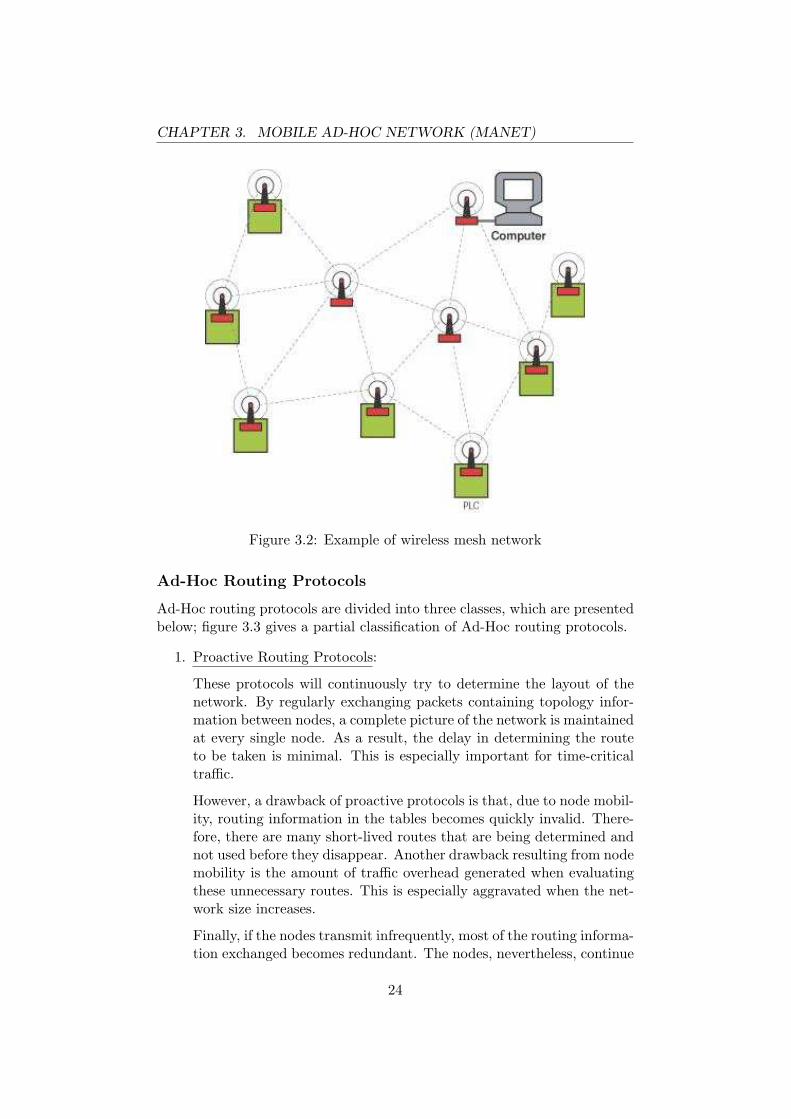
Wireless mesh networks is a category of networks immediately derivedfrom MANETs. In these types of networks, nodes cooperate to relay amessage to its destination. Each node has a set of neighbors which it can useto forward messages; this way, if a neighbor disappears (i.e. node movement,node switched off) the node can just pick another neighbor and continue tohave access to the network. This feature makes wireless mesh networksextremely reliable and scalable. What’s more, a way to increase reliabilityis simply to add nodes which increases the number of neighbors and thereforemeans more possibilities for a node to forward messages. Figure 3.2 givesan example of a wireless mesh network.
As seen in figure 3.2, one of the nodes of the network can be a basestation or another device connected to the Internet for instance. This allowsnodes to send packets over the Internet even though they are not withinreach of the base station’s signal. This characteristic is the reason why thiswork puts forward a solution that relies on Ad-Hoc networking.
3.2 Ad-Hoc Routing3
As mentioned above, wired networks routing algorithms cannot be used”as-is” in wireless Ad-Hoc networks due to the mobility of the nodes. Thebasic routing principals such as Distance-Vector and Link-State have to beadapted to Ad-Hoc networking by taking into account that neighbors couldappear and disappear at any moment. This section will present differentrouting algorithms used within Ad-Hoc networks, including AODV4 whichis used in this work.
3Protocol and algorithm will have the same meaning in this section4Ad-Hoc On Demand Distance Vector
23
CHAPTER 3. MOBILE AD-HOC NETWORK (MANET)
Figure 3.2: Example of wireless mesh network
Ad-Hoc Routing Protocols
Ad-Hoc routing protocols are divided into three classes, which are presentedbelow; figure 3.3 gives a partial classification of Ad-Hoc routing protocols.
1. Proactive Routing Protocols:
These protocols will continuously try to determine the layout of thenetwork. By regularly exchanging packets containing topology infor-mation between nodes, a complete picture of the network is maintainedat every single node. As a result, the delay in determining the routeto be taken is minimal. This is especially important for time-criticaltraffic.
However, a drawback of proactive protocols is that, due to node mobil-ity, routing information in the tables becomes quickly invalid. There-fore, there are many short-lived routes that are being determined andnot used before they disappear. Another drawback resulting from nodemobility is the amount of traffic overhead generated when evaluatingthese unnecessary routes. This is especially aggravated when the net-work size increases.
Finally, if the nodes transmit infrequently, most of the routing informa-tion exchanged becomes redundant. The nodes, nevertheless, continue
24

CHAPTER 3. MOBILE AD-HOC NETWORK (MANET)
Figure 3.3: Partial Ad-Hoc Routing Protocols Classification
to use up energy by continually updating these unused entries in theirrouting tables which diminishes battery autonomy.
Hence, proactive protocols work best in networks that have low nodemobility or where the nodes transmit data frequently or when powerconsumption is not an issue.
Examples of proactive protocols are:
DSDV[9], Dynamic Destination-Sequenced Distance-Vector Routing.This protocol is based on the classical Bellman-Ford routing algorithm.Each node maintains a list of all destinations and number of hops toeach destination. Each entry is marked with a sequence number. Ituses full dump (whole routing table) or incremental packets to reducenetwork traffic generated by route updates. The broadcast of routeupdate is delayed by settling time. The Distributed Bellman-Ford hasthe looping and count-to-infinity problem, which is avoided in DSDVby using sequence numbers.
DSDV requires a full dump update periodically, therefore DSDV isnot efficient in route updating. DSDV limits the number of nodes thatcan join the network. Whenever the topology of a network changes,DSDV is unstable until update packets propagate through the network.DSDV is effective for creating ad-hoc networks for small populationsof mobile nodes.
DSDV is a well-known routing algorithm for ad-hoc network routing.
25

CHAPTER 3. MOBILE AD-HOC NETWORK (MANET)
Because there are no standard specifications, no commercial imple-mentations are available. Many improved protocols based on DSDVhave been developed such as AODV.
Another example of proactive routing protocol is OLSR[10] whichstands for Optimized Link State Routing Protocol. In this protocol,every node periodically sends broadcast ”Hello”messages with informa-tion to specific nodes in the network to exchange neighborhood infor-mation. Included in these ”Hello”messages, are the nodes IP, sequencenumber and a list of the distance information of the nodes neighbors.After receiving this information a node builds itself a routing table.The node can then calculate the route to every node using the short-est path algorithm. When a node receives an information packet withthe same sequence number twice it is discarded. The information inthe routing table is updated when a change in the neighborhood isdetected, or a route to any destination is expired or when a better(shorter) route is detected for a destination.
The key concept used in the protocol is that of multipoint relays(MPRs). MPRs are selected nodes which forward broadcast mes-sages during the flooding process. This technique substantially reducesthe message overhead as compared to a classical flooding mechanism,where every node retransmits each message when it receives the firstcopy of the message. In OLSR, link state information is generated onlyby nodes elected as MPRs. Thus, a second optimization is achievedby minimizing the number of control messages flooded in the network.As a third optimization, an MPR node may chose to report only linksbetween itself and its MPR selectors. Hence, contrary to the classiclink state algorithm, partial link state information is distributed in thenetwork. This information is then used for route calculation. OLSRprovides optimal routes (in terms of number of hops). The protocol isparticularly suitable for large and dense networks as the technique ofMPRs works well in this context.
2. Reactive Routing Protocols:
These kind of protocols only find a route to the destination node whenthere is a need to send data. The source node will start a route discov-ery procedure by transmitting route requests throughout the network.The sender will then wait for a response from the destination node oran intermediate node (that has a route to the destination) which willinclude a list of intermediate nodes between the source and destination.
The main drawback is that route discovery generates a significant delaybefore the packet can be transmitted. It also requires the transmissionof a significant amount of control traffic.
26

CHAPTER 3. MOBILE AD-HOC NETWORK (MANET)
Hence, reactive protocols are most suited for networks with high nodemobility or where the nodes transmit data infrequently.
An example of such a protocol is DSR[11] or Dynamic Source Routing.This protocol is based on the concept of source routing. Mobile nodesare required to maintain route caches that contain the routes knownby the node. Entries in the route cache are continually updated asnew routes are learned. The protocol is composed of the two mainmechanisms: ”Route Discovery”and ”Route Maintenance”, which worktogether to allow nodes to discover and maintain routes to arbitrarydestinations in the ad hoc network. To limit the bandwidth used, theprocess to find a route to a destination is only executed when needed.All aspects of the protocol operate entirely on-demand which impliesthat DSR is beacon-less, unlike some other reactive protocols such asABR5 for instance. There are no ”Hello”messages used between nodesto notify their neighbors about their presence. In DSR the sender(source, initiator) determines the whole path from the source to thedestination node (Source-Routing) and inserts the addresses of theintermediate nodes used along the route in the packets it sends.
The protocol allows multiple routes to any destination and allows eachsender to select and control the routes used in routing its packets, forexample for use in load balancing or for increased robustness. Otheradvantages of the DSR protocol include easily guaranteed loop-freerouting, operation in networks containing unidirectional links and veryrapid recovery when routes in the network change.
DSR also suffers from a scalability problem due to the nature of sourcerouting. As the network becomes larger, the control packets and mes-sage packets also become larger. This gives a negative impact due tolimited bandwidth. Also packets may be forwarded along stale cachedroutes.
Hence, DSR works best in networks with a small diameter (between 5and 10 hops) and the nodes should only move around at a moderatespeed.
TORA[12], Temporally-Ordered Routing Algorithm is another exam-ple of reactive routing protocol. This protocol is a highly adaptive,loop-free, distributed routing protocol based on the concept of linkreversal. It is source initiated and provides multiple routes for anydesired source/destination pair. There are 3 basic functions of theprotocol: route creation, route maintenance and route erasure.
Since this protocol uses internodal co-ordination it exhibits instabil-ity behavior similar to ”count-to-infinity” problem in distance vector
5Associativity Based Routing
27

CHAPTER 3. MOBILE AD-HOC NETWORK (MANET)
routing protocols. There is a potential for oscillations to occur, espe-cially when multiple sets of coordinating nodes are concurrently detect-ing partitions, erasing routes, and building new routes based on eachother. Though, such oscillations are temporary and route convergencewill ultimately occur.
Finally, AODV6[1]: Ad Hoc On-Demand Distance Vector Routing Pro-tocol is one of the most used Ad-Hoc routing protocol. It is a reactiverouting protocol based on DSDV. AODV is designed for networks withtens to thousands of mobile nodes. One feature of AODV is the use ofsequence numbers in order to insure loop freedom. Sequence numbersare used by other nodes to determine the freshness of routing informa-tion. If a node has the choice between two routes to a destination, anode is required to select the one with the greatest sequence number.
In AODV, every node has a routing table. As with DSR, the pro-cess to find a route to a destination is only executed when neededusing RREQs (Route Request) messages originating from the sourcenode and RREPs (Route Reply) messages sent by the destination orintermediate nodes which have a route to the destination. AODValso implements a ”Route Repair” mechanism which enables a node toswitch to a different route if an intermediate node along the originalroute goes down.
3. Hybrid Routing Protocols:
Since proactive and reactive routing protocols each work best in oppo-sitely different scenarios, there is good reason to develop hybrid routingprotocols, which use a mix of both proactive and reactive techniquesprotocols. These hybrid protocols can be used to find a balance be-tween the proactive and reactive protocols.
The basic idea of hybrid routing protocols is to use proactive rout-ing mechanisms in some areas of the network at certain times andreactive routing for the rest of the network. The proactive operationsare restricted to a small domain, called the zone radius, in order toreduce the control overheads and delays. The reactive routing proto-cols are used for locating nodes outside this domain, as this is morebandwidth-efficient in a constantly changing network.
The perfect example of a hybrid routing protocol is ZRP[13]: ZoneRouting Protocol. In this protocol, the radius of each node’s localrouting zone plays an important part in determining the proactivezone. The proactive mechanism is used to determine the topology
6This is a brief summary of this protocol, it will be more widely discussed in the secondpart of this work (Personal Contribution).
28

CHAPTER 3. MOBILE AD-HOC NETWORK (MANET)
within the radius of the node. The reactive routing protocol is thenused to locate nodes outside the radius of the node on demand.
The adjustment of the zone radius will allow the protocol to adapt todifferent network environments. A larger radius will favor the proac-tive routing protocol, optimal for slow-moving nodes or large amountsof traffic. Consequently, a smaller zone radius will favor the reactiveprotocol, which is optimal for fast-moving nodes or small amounts oftraffic.
29

Chapter 4
Interconnecting Ad-Hoc andCellular Networks
4.1 Existing Solutions
Two existing systems will be presented in this section to illustrate the ben-efits of interconnecting Ad-Hoc and Cellular networks:
• iCAR[21] which addresses the congestion problem due to unbalancedtraffic in a cellular system and provides interoperability for heteroge-neous networks and
• UCAN[22], an architecture designed to enhance cell throughput, whilemaintaining fairness1.
4.1.1 iCAR
iCAR or Integrated Cellular and Ad hoc Relaying System is a relatively newsolution introduced in 2002 by Hongyi Wu.
This system makes use of Ad-Hoc Relay Stations (ARS) which are lightweight2versions of a cellular network’s base station. These relay stations are capa-ble of communicating directly with a cellular network base station, mobilehosts and other relay stations. The difference between standard base sta-tion and an ARS is that this relay station is a wireless device whereas abase station is usually connected to a controlling equipment (i.e. a BTSconnected to a MSC in GSM) using wires. In addition ARS’s are capableof limited mobility which allows an operator to move its ARS to strategicareas in order to adapt to changing situations.
1Providing service to low data-rate users is required for maintaining fairness, but atthe cost of reducing the cell’s aggregate throughput
2literally and in terms of complexity
30

CHAPTER 4. INTERCONNECTING AD-HOC AND CELLULARNETWORKS
Three main relaying situations involve these relay stations and mobile hosts:
• Primary Relaying: If a mobile host is unable to obtain a channel ina congested cell, it can be relayed to a neighboring cell using an ARSif the mobile host is within the coverage area of an ARS. This case isillustrated by figure 4.1.
Figure 4.1: Primary Relaying
• Secondary Relaying: In this type of relaying, the objective is to free achannel of a congested base station so it can be attributed to a mobilehost located outside the coverage area of any ARS. Two cases arepossible:
– Either an on-going connection by a mobile host in the vicinity ofan ARS is transferred to another cell which frees up a channel.
Figure 4.2: Case one of Secondary Relaying
– Or a call between two mobile hosts, one located in the congestedcell and the other located either in the same cell or a neighbor-ing cell, is relayed through ARS’s allowing other mobile hosts toacquire channels.
• Cascaded Relaying: This type of relaying uses both previously de-scribed relaying techniques and spans multiple cells. The idea is that
31

CHAPTER 4. INTERCONNECTING AD-HOC AND CELLULARNETWORKS
Figure 4.3: Case two of Secondary Relaying
if neither primary or secondary relaying is possible3, a neighboring cellwill free up a channel through primary relaying which will then enablesecondary relaying in the originating cell by using the newly freed upchannel. Figure 4.4 illustrates this case, MH Z frees up a channel incell C via primary relaying which makes it possible to free a channelin cell B for MH X using secondary relaying.
Figure 4.4: Cascaded Relaying
In the cases presented above, the reason for using an ARS is conges-tion in a cell. However these mechanisms can also be applied in situationsmentioned earlier, where dead spots are encountered but where the host isstill in the coverage area of an ARS. The main difference between the iCAR
3neighboring cells could also be congested
32

CHAPTER 4. INTERCONNECTING AD-HOC AND CELLULARNETWORKS
system and the one presented in this work is that in this work, the stationsused to relay communications have the same mobility properties as regularmobile hosts.
4.1.2 UCAN
The Unified Cellular and Ad-Hoc Network Architecture is a system designedfor interworking between 802.11 and third-generation wireless data networks.
In this system, a UE realizing that it currently has a low signal-to-noiseratio, and thus a low data rate, can turn to other UEs having a better SNR4
to forward its traffic.In UCAN, the protocol which determines which UE has the best SNR
ratio in order to forward traffic using the Ad-Hoc network is called ”ProxyDiscovery”. Two different protocols are available: Greedy (which is proac-tive) and On-Demand (which is reactive). As with AODV for example, aroute repair protocol is also implemented.
Figure 4.5 illustrates the use of UCAN.
Figure 4.5: Example of UCAN use
4Signal-to-Noise Ratio
33
CHAPTER 4. INTERCONNECTING AD-HOC AND CELLULARNETWORKS
4.1.3 Conclusion
Much work has been done in the area of interconnecting Cellular and Ad-Hoc networks. Aside from the couple of solutions presented in this chap-ter, many other systems have been developed, especially for disaster crisismanagement. Here are some references to other interconnection systems:[23][25][24]
4.2 Motivations of this study
This study focuses on providing cellular network access to mobile hosts, inan indoor environment, which are out of range of any base station. In otherwords, the object of this work is to extend the coverage of a cellular networkusing Ad-Hoc networking.
4.2.1 Propagation Issues5
As we have seen in the chapter concerning cellular networks, mobile hostsin such systems can be deprived of network access if reception from a basestation is impossible. This section will examine the reasons why such asituation should arise, particularly indoors.
Basic Radio Propagation
The most basic model of radio wave propagation involves the so called ”freespace” or ”Strong Line Of Sight” radio wave propagation. In this model,radio waves originate from a source of radio energy and travel in all direc-tions in a straight line, filling the entire spherical volume of space with radioenergy that varies in strength with respect to the power of the distance6
(or 20 dB per decade increase in range). This means that if you double thedistance over which you transmit, the received power will be reduced by afactor of 4. As an example, figure 4.6 shows the amount of power receivedwhen one Watt of power is transmitted over the air.
5This section was inspired by [14] and [15]6Theoretical formula: Pr
Pe=( λ
4πd)n with n≥ 2
34
CHAPTER 4. INTERCONNECTING AD-HOC AND CELLULARNETWORKS
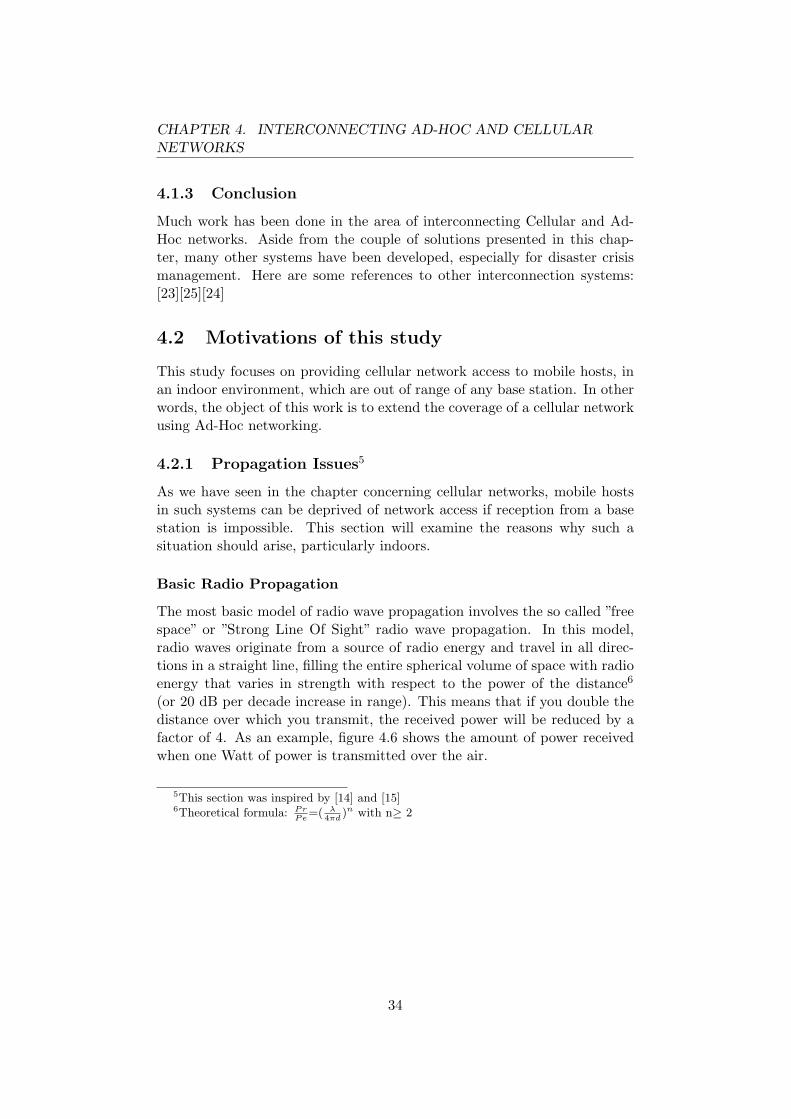
Transmission Range (d) Average Power Received1 meter 0.00002 Watts5 meters 0.0000013 Watts10 meters 0.0000004 Watts1000 meters 0.000000000158 Watts
Figure 4.6: Average power received when transmitting one Watt of powerusing the free space model
To provide a comparison, when transmitting 1 Watt of power over a fiberoptic cable that is 1000 meters long, on average, 0.933 Watts of power isreceived.
Real world radio propagation rarely follows this simple model. The threebasic mechanisms of radio propagation are attributed to reflection, diffrac-tion and scattering. All three of these phenomena cause radio signal distor-tions which in turn result in signal fades, as well as additional signal prop-agation losses. Outdoors, movements over very small distances by mobilehosts give rise to signal strength fluctuations because the composite signalreceived is made up of a number of components from the various sources ofreflections (called ”multipath signals[16]”) from different directions as well asscattered and/or diffracted signal components. These signal strength vari-ations amount to as much as 30 to 40 dB in frequency ranges useful formobile communications and account for some of the difficulty presented tothe designer of reliable radio communications systems. The basic signal at-tenuation with range noticed in the real world gives rise to what are termed”large scale” effects, while the signal strength fluctuations with motion aretermed ”small scale” effects.
Multipath Signals
In order for the free space model to be applicable, the antennas of commu-nicating devices need to see each other. In urban areas and especially inindoor environments such a situation is highly improbable.
In the real world, multipath occurs when there is more than one pathavailable for radio signal propagation. The phenomena of reflection, diffrac-tion and scattering all add radio propagation paths to the initial direct ”lineof sight” path between the transmitter and receiver.Here is the description of these three phenomena by Theodore S. Rappaport[17]:
• Reflection occurs when a propagating electromagnetic wave impingesupon an object which has very large dimensions when compared tothe wavelength of the propagating wave. Reflections occur from thesurface of the earth and from buildings and walls.
35

CHAPTER 4. INTERCONNECTING AD-HOC AND CELLULARNETWORKS
• Diffraction occurs when the radio path between the transmitter andreceiver is obstructed by a surface that has sharp irregularities (edges).The secondary waves resulting from the obstructing surface are presentthroughout the space and even behind the obstacle, giving rise to abending of waves around the obstacle, even when a line-of-sight pathdoes not exist between transmitter and receiver. At high frequencies,diffraction, like reflection, depends on the geometry of the object, aswell as the amplitude, phase, and polarization of the incident wave atthe point of diffraction.
• Scattering occurs when the medium through which the wave travelsconsists of objects with dimensions that are small compared to thewavelength, and where the number of obstacles per unit volume islarge. Scattered waves are produced by rough surfaces, small objects,or by other irregularities in the channel. In practice, foliage, streetsigns, and lamp posts induce scattering in a mobile communicationssystem.
Multiple signal propagation paths are caused by any of the above phe-nomenon. The actual received signal level is the vector sum of all the signalsincident from any direction or angle of arrival. Some signals will aid the di-rect path, while other signals will subtract (or tend to vector cancel). Thetotal composite phenomenon is thus called multipath. Two kinds of mul-tipath exist: specular multipath arising from discrete, coherent reflectionsfrom smooth metal surfaces; and diffuse multipath arising from diffuse scat-terers and sources of diffraction (the visible glint of sunlight off a choppy seais an example of diffuse multipath).
Both forms of multipath are bad for radio communications. Diffuse mul-tipath provides a sort of background ”noise” level of interference, while spec-ular multipath can actually cause complete signal outages and radio ”deadspots” within a building. This problem is especially difficult in undergroundpassageways, tunnels, stairwells and small enclosed rooms.
Figure 4.7 presents an example of multipath signal.
• Path 1: Is a line-of-sight path. The amount of power we receive at themobile host depends only on the distance between the two devices.
• Path 2: Is a path that is the result of a reflection off an object. Herewe will lose power over the length of the path from the base stationto the object, and over the length of the path from the object to themobile host. It is very important to note that, in this case, we are notpropagating over the distance between the base station and the mobileunit but over the total length of Path 2. In addition, the object willalso absorb some of the energy of the signal before it is reflected. Theamount that it absorbs depends on the material of that object.
36

CHAPTER 4. INTERCONNECTING AD-HOC AND CELLULARNETWORKS
Figure 4.7: Example of multipath signal
• Path 3: Similar to Path 2, we have the signal reflecting off an ob-ject on its way from the base station to the mobile host. Notice alsothat it passes through another object on its way to the mobile unit.The amount of power that is reduced as it passes through the objectdepends again on the material of that object.
In this example the mobile will receive so much power from Path 1,since it did not reflect or pass through any object, and because it was theshortest of the three paths, that we can ignore Paths 2 and 3. However,in many situations, we do not have direct line-of-sight between devices andcommunication between them can only be made possible through indirectpaths like 2 and 3.
Indoor Radio Propagation
Indoor radio propagation is characterized with the same effects as outdoorpropagation: reflection, diffraction, and scattering. But the influence of eachparameter is much greater for indoor propagation. The behavior of radiosignals in buildings depends on the working frequency, the building layout,the construction materials used and the building type. Walls and obstaclessuch as desks and partitions, made of different materials obstruct the signal
37

CHAPTER 4. INTERCONNECTING AD-HOC AND CELLULARNETWORKS
differently. Therefore, it is very difficult to design an ”RF7 friendly”buildingthat is free from multipath reflections, diffraction around sharp corners orscattering from wall, ceiling, or floor surfaces (needless to say that perfectoperation is nearly impossible in existing buildings). The best case scenariofor an ”RF friendly” building would be an all wooden or all fiberglass struc-ture but even then such a building will still have reflections, multipath andother radio propagation disturbances which will prove to be less than ideal.
Inside smooth walled metal buildings, radio wave propagation can beso bad that ”dead spots” can appear, where the signal is virtually non-existent. The reason for this is because of almost perfect, lossless reflectionsfrom smooth metal walls, ceilings or fixtures that interfere with the directradiated signals. The dead spots exist in three dimensional space within thebuilding, and movements of only a few centimeters can alter reception fromno signal to full signal.
Radio wave propagation obstacles are divided into two categories: hardpartitions if they are part of the physical/structural components of a buildingand soft partitions which are formed by the office furniture and fixed ormovable/portable structures that do not extend to a buildings ceiling. Radiosignals effectively penetrate both kinds of partitions in ways that are veryhard to predict.
An obstacle with a measured loss of 20dB or more from its materialsis a significant loss if you consider the free space model where 20db is theadditional loss reported per decade increase in range. The equivalent to atransparent object in radio wave propagation would consist of a materialwith a three to six dB loss.
In order to predict the signal level inside a building, different parametershave to be considered8:
• Building penetration caused by the signal entering the building. It hastwo main factors: wall penetration and window area. It is found thatthe wall penetration for 900 MHz signals can be in the range 15 - 27dB, depending on building construction. The building penetration inthe window area is approximately 6 dB.
• Floor attenuation depends on the number of floors between the trans-mitter and receiver, the type of the material, and the working fre-quency. It is found that for the carrier frequency of 900 MHz, theattenuation in the first thirteen floors is nearly the same, about 2.7dB/floor. Above thirteen floors the attenuation is approximately 7dB/octave.
7Radio Frequency8see [17] for a detailed description on signal attenuation inside buildings
38

CHAPTER 4. INTERCONNECTING AD-HOC AND CELLULARNETWORKS
For both factors, we can extrapolate this data for use at around 2GHz, whichis used for UMTS, if we add a few dB (perhaps 5 to 6 dB) to account forthe higher frequency.
Propagation Models
Two different propagation models will be used in this work:
1. The Freespace Model[18]:
The free space propagation model assumes the ideal propagation con-dition that there is only one clear line-of-sight path between the trans-mitter and receiver. H. T. Friis presented the following equation tocalculate the received signal power in free space at distance d from thetransmitter[20].
Pr(d) =PtGtGrλ
2
(4π)2d2L(4.1)
where Pt is the transmitted signal power. Gt and Gr are the antennagains of the transmitter and the receiver respectively. L(L ≥ 1) is thesystem loss, and λ is the wavelength.
The free space model basically represents the communication range asa circle around the transmitter. If a receiver is within the circle, itreceives all packets. Otherwise, it loses all packets.
2. The Shadowing Model[19]:
The shadowing model consists of two parts. The first one is knownas the path loss model, which also predicts the mean received powerat distance d, denoted by Pr(d). It uses a close-in distance d0 as areference.Pr(d) is computed relative to Pr(d0) as follows.
Pr(d0)Pr(d)
=(
d
d0
)β
(4.2)
β is called the path loss exponent, and is usually empirically deter-mined by field measurement. From Eqn. (4.1) we know that β = 2for free space propagation. Larger values correspond to more obstruc-tions and hence faster decrease in average received power as distancebecomes larger. Pr(d0) can be computed from Eqn. (4.1).
39

CHAPTER 4. INTERCONNECTING AD-HOC AND CELLULARNETWORKS
The path loss is usually measured in dB. So from Eqn. (4.2) we have[
Pr(d)Pr(d0)
]
dB
= −10βlog(
d
d0
)(4.3)
The second part of the shadowing model reflects the variation of thereceived power at certain distance. It is a log-normal random variable,that is, it is of Gaussian distribution if measured in dB. The overallshadowing model is represented by
[Pr(d)Pr(d0)
]
dB
= −10βlog(
d
d0
)+ XdB (4.4)
where XdB is a Gaussian random variable with zero mean and standarddeviation σdB. σdB is called the shadowing deviation, and is alsoobtained by measurement. Eqn. (4.4) is also known as a log-normalshadowing model.
The shadowing model extends the ideal circle model to a richer statisticmodel: nodes can only probabilistically communicate when near theedge of the communication range.
Conclusion
As we have seen indoor radio propagation is extremely variable and tremen-dously tricky to predict (sometimes even impossible). Using a cellular systemsuch as UMTS it is inevitable to encounter some dead spots (basements orparking lots are common examples) inside buildings where no reception ispossible. For mobile hosts which find themselves in such situations, Ad-Hocnetworking can be of valuable assistance. Instead of having mobile unitsdeprived of any connectivity, using a Ad-Hoc approach these hosts can finda route, made up of other mobile hosts, ending with a host connected to thecellular network. This would then allow the node to enjoy the services ofthe cellular network even though no base station signal is available. This iscalled coverage extension.
Figure 4.8 illustrates this solution.In this figure:
• Mobile host 1 has direct access to the cellular network through a basestation.
• Mobile hosts 2 and 3 on the other hand have to go through host 1 tohave access to the cellular network.
40

CHAPTER 4. INTERCONNECTING AD-HOC AND CELLULARNETWORKS
Figure 4.8: Cellular network assisted by Ad-Hoc networking
41

Part II
Personal Contribution
42

Introduction
This part will describe a new solution for extending a cellular network (i.e.a 3G network in this case) using Ad-Hoc networks and suitable for an indoorenvironment.
To start with, a more detailed description of AODV (see chapter 3) willbe presented along with the ABR (Associativity Based Routing) protocol.Then, the hypotheses and assumptions made for this study will be presented.After that, the modifications and additions to AODV named GWAODV9,will be detailed and finally NS-2, the network simulator used to evaluatethis new protocol along with the results it generated will be explained.
9GWAODV: Gateway Ad-Hoc On-demand Distance Vector
43

Chapter 5
AODV: Ad-hoc On-demandDistance Vector
As mentioned earlier, AODV[1] is a reactive routing protocol which meansthat an unknown route is discovered only when needed. However, unlikeDSR, AODV makes use of beacon messages so that nodes can maintain alist of immediate neighbours. These messages are sent with a time-to-live ofone to prevent distribution past immediate neighbours.
Route repair mechanisms allow routes to be reconstructed if an interme-diate node goes down. This feature makes it possible for AODV to adapt toa changing network topology.
In order to avoid routing loops and count-to-infinity problems associatedwith classical distance vector algorithms, AODV uses sequence numberswhich are included in every route information message.
5.1 Message Types
There are three different messages in AODV:
• RREQ: Route Request which is sent when a route for an unknowndestination is required
• RREP: Route Reply which is sent as a reply to a RREQ either by thedestination itself or an intermediate node which has an active route toa destination.
• RERR: Route Error which is sent when a node realizes that a neigh-bour is no longer reachable.
An additional beacon or ”Hello” message is also used to notify immediateneighbours of the node’s presence, these messages are periodically sent to anode’s neighbours.
44

CHAPTER 5. AODV: AD-HOC ON-DEMAND DISTANCE VECTOR
5.2 AODV Operation
This is a simplified description of the operation of AODV. For a completeunderstanding of this protocol, please see [1].
5.2.1 Sequence Numbers
A sequence number is maintained in every node; it is incremented beforesending out either a RREQ or a RREP. When a route is entered in a node’srouting table, it also records the destination’s sequence number containedin the RREQ message. This destination sequence number has to be thelatest sequence number available to prevent loops if the information is stale.A node changes the destination sequence number of a routing table entrywhen:
• it is itself the destination and it offers a new route to itself
• it receives a message with new information about the sequence numberof the destination
• the path towards the destination expires or breaks
5.2.2 Routing Table
The routing table of a node contains the following information for each route:
• Destination IP address
• Destination Sequence Number: The destination sequence number as-sociated with the route.
• Next Hop: The IP address of either the destination or an intermediatenode along the route to the destination.
• Hop Count: The number of hops from the source to the destination.
• Flags: State of the route; valid (currently being used), invalid (notused at the moment but still in cache for information purposes) orbeing repaired.
• Lifetime: For an active route this field denotes the time at which theentry becomes invalid (expiry time). For invalid routes it representsthe deletion time.
An entry of the routing table is created whenever a node receives a messagefor an unknown destination.An entry is updated when:
• a message with a higher destination sequence number is received
45
CHAPTER 5. AODV: AD-HOC ON-DEMAND DISTANCE VECTOR
• a message with the same destination sequence number is received butwith a smaller hop count
• the destination sequence number is null (i.e. unknown) and a messagecontaining a sequence number for that destination is received
• a message with the same destination sequence number is received andthe route is invalid (update of deletion time)
5.2.3 Route Discovery
Creating a RREQ
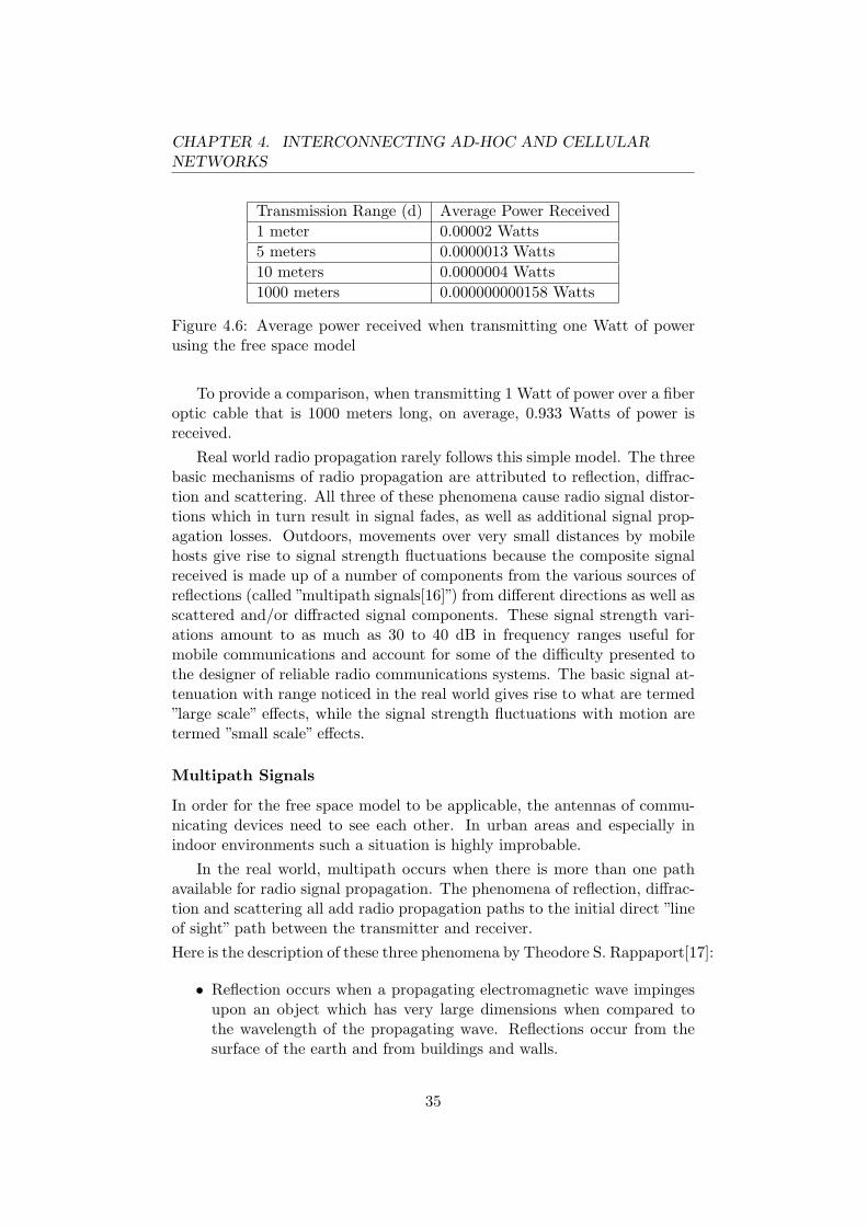
A node initiates a route discovery phase by generating a RREQ. This phaseis needed when a node wishes to communicate with a previously unknowndestination or a destination for which its routing table entry has becomeinvalid. As an example, in figure 5.1, node 1 wants to exchange informationwith node 4 but it doesn’t have a route to that destination. Node 1 will
Figure 5.1: Example of the need of a route discovery phase
then construct a RREQ message containing:
• a RREQ ID which allows nodes to discard requests they have alreadyseen, it’s incremented by the source node before each new RREQ
46
CHAPTER 5. AODV: AD-HOC ON-DEMAND DISTANCE VECTOR
• Destination IP address and sequence number
• Originator IP address and sequence number which is incremented be-fore insertion
• a Hop Count of 0
• an empty list of IP address-sequence number pairs (path list) whichwill be updated by nodes receiving this RREQ so that the RREPmessage will know the route back to the originator
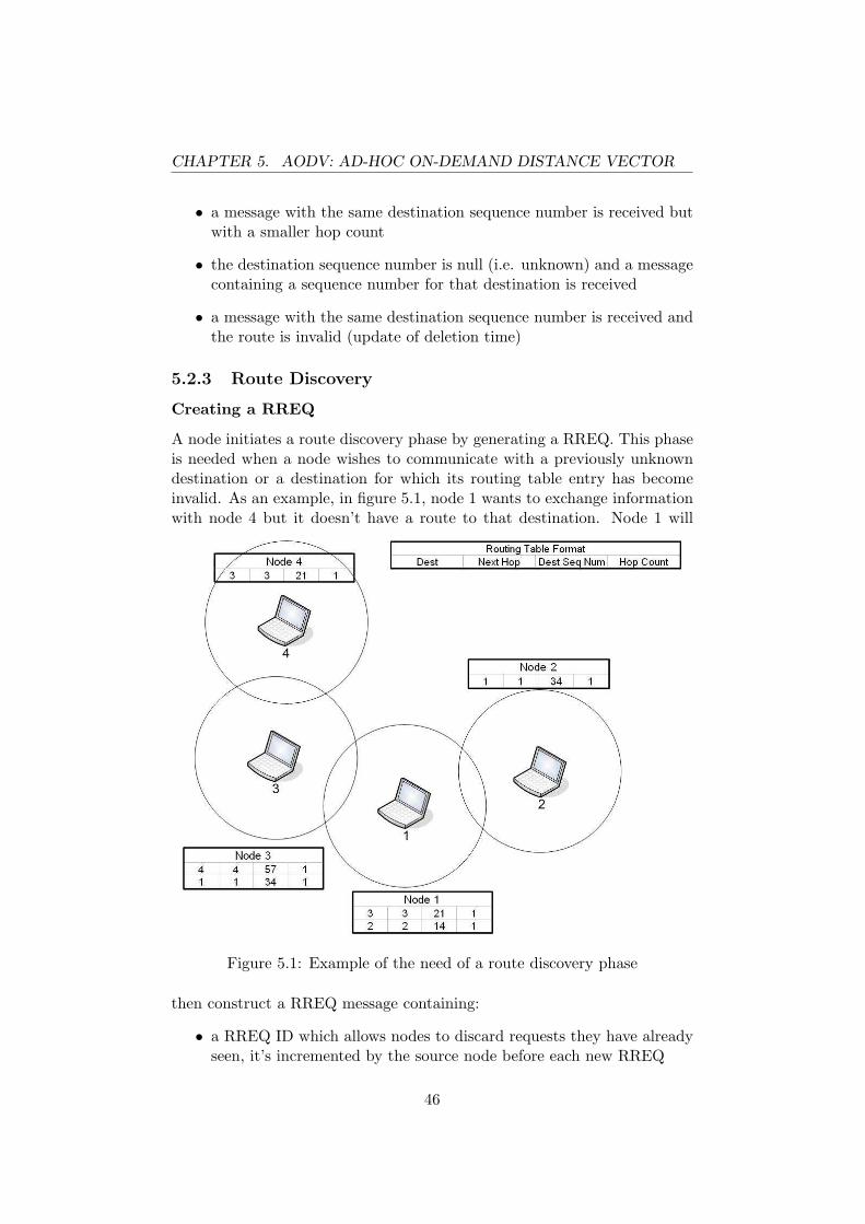
Once this RREQ is generated, the node saves this message in a buffer toavoid reprocessing or re-forwarding this RREQ if it receives it from a neigh-bour and broadcasts the message. Figure 5.2 illustrates this process.
Figure 5.2: RREQ creation and distribution
Receiving a RREQ
Node 2 and 3 will receive this RREQ. Both nodes will increase the hop countfield by one. As a general rule, each node receiving this RREQ may create
47

CHAPTER 5. AODV: AD-HOC ON-DEMAND DISTANCE VECTOR
or update a route to any destination listed in the path list included in theRREQ. Since node 2 and 3 are neighbours of node 1, this list is empty andno modifications are made to their routing table.
Next, each node checks if they have already received a RREQ from thesame source with the same RREQ ID. If such a RREQ has been received,the node discards the newly received RREQ.
Otherwise, two options are available depending on the presence or not ofa route to the destination in a node’s routing table. Node 2 and 3 illustratethese two possibilities.
Forwarding a RREQ
Node 2 has no routing table entry for node 4. If the time-to-live field of theIP header is greater than one then node 2 will rebroadcast this RREQ. Priorto this node 2 has to decrease the time-to-live field of the IP header by oneand append its own IP address and sequence number to the path list of theRREQ.
Creating a RREP
Node 3 on the other hand is a neighbour of node 4 and its routing tablecontains an entry for that destination. Therefore node 3 is able to respondto the RREQ through a RREP which contains:
• the Destination Sequence Number found in its routing table
• the Destination IP address, Originator IP address and Originator Se-quence number extracted from the RREQ.
• the hop count field of the routing table is copied in the RREP
• the path list of the RREQ is included in the RREP in the same orderas in the RREQ
The RREP can now be unicast to next hop towards the originator, indicatedby the last entry in the path list.Figure 5.3 demonstrates this process. The RREQ forwarded by node 2 andwhich reaches node 1 is not represented on the figure for clarity.
Receiving a RREP
When a node receives a RREP message, it increments the Hop Count field.Then it may update or create an entry for the Destination IP(i.e. node 4in this case) of the RREP and any other node in the path list. If the nodereceiving the RREP is not the destination, it has to forward the message tothe previous node in the path list (the path list is read in reverse order).
48

CHAPTER 5. AODV: AD-HOC ON-DEMAND DISTANCE VECTOR
Figure 5.3: RREQ forwarding and RREP creation
In this example, node 1 increments the Hop Count and updates its routingtable. It now has an active route to node 4 (See figure 5.3 for node 1’srouting table).
5.2.4 Route Repair and RERR
RERR
A node generates a RERR message in three situations:
1. The node detects a link break for the next hop of an active route in itsrouting table while transmitting data (and route repair, if attempted,was unsuccessful).
2. The node receives a data packet for an invalid route or an unknowndestination.
3. The node receives a RERR from a neighbor for one or more activeroutes.
This RERR message will contain a list of unreachable destinations accordingto the situation which arises.For the first case, the node creates a list of unreachable destinations con-sisting of the unreachable neighbor and any additional destination present
49

CHAPTER 5. AODV: AD-HOC ON-DEMAND DISTANCE VECTOR
in the node’s routing table and using the unreachable neighbor as the nexthop.In case 2, there is only one unreachable destination, which is the destinationof the data packet that cannot be delivered.In the last case, the list should consist of those destinations in the RERRfor which there exists an entry in the node’s routing table that has thetransmitter of the received RERR as the next hop.In all cases, a node will invalidate any route where the destination is presentin the unreachable destination list. The node will then broadcast this mes-sage to all its neighbours.
Local Repair
When a link break in an active route occurs, the node upstream of the breakcan choose to repair the link locally if the destination is no farther than acertain amount of hops. To repair the link break, the node increments thesequence number for the destination and begins a route discovery phase buton a smaller scale than the original RREQ1.
If at the end of the discovery period, the repairing node has not received aRREP (or other control message creating or updating the route) it transmitsa RERR message for that destination as seen in the previous section.
On the other hand, if the node receives one or more RREPs (or othercontrol message creating or updating the route to the desired destination)during the discovery period, it can update its route table entry for thatdestination. The node can now use this active route to forward data packets.
Local repair of link breaks in routes enables nodes to maintain communi-cation while the network topology changes. However this process sometimesresults in an increased path length to a destination.
1the time-to-live field is set for a smaller distribution radius
50

Chapter 6
ABR: Associativity-BasedRouting
ABR is a reactive and beacon-based routing protocol. It was developed byC.K. Toh at Cambridge University in 1996. This protocol selects routesbased on the temporal stability of the links between the nodes. The funda-mental objective is to find longer-lived routes.
Each node generates periodic beacons (hello messages) to signify its ex-istence to its neighbors. These beacons are used to update the associativitytable of each node. This table contains the associativity level between anode and its neighbours. With the temporal stability and the associativitytable the nodes are able to classify each neighbor link as stable or unstable.
Stability is determined using ”associativity ticks”. Association in ABR isbased on a few metrics such as link delay, signal strength, power life, routerelaying load, period of presence or spatial and temporal characteristics.Routes are only chosen when they have a high degree of associativity whichmeans a high level of associativity ticks.
6.1 ABR Operation
The ABR protocol consists of three phases; route discovery, route recon-struction and route deletion.
6.1.1 Route Discovery
If a node has in his Route Cache a route to the desired destination then thisroute is immediately used. If not, the Route Discovery protocol is started.
First the network is flooded with RouteRequest messages originatingfrom the source. These messages are only forwarded once by each interme-diate node. When receiving a RouteRequest message, intermediate nodesappend their address and associativity ticks to the packet.
51

CHAPTER 6. ABR: ASSOCIATIVITY-BASED ROUTING
Once the RouteRequest message reaches the destination node, this nodewill wait a certain period of time during which it may receive other RouteRequestmessages from the same source but delivered along different routes. It willthen select the best route by examining the associativity ticks along eachpath. If multiple routes have the same overall degree of stability, the routewith the minimum number of hops will be selected.
After the route as been chosen, the destination sends a Reply packetback to the source along the same path.Figure 6.1 illustrates this process.
Figure 6.1: ABR Route Discovery
Three routes are possible from 1 to 15:
• 1-5-10-14-15
• 1-5-4-12-15
• 1-2-4-8-13-15
ABR selects the last route because of the highest percentage of stable linkson this path.
6.1.2 Route Repair
As with Local Repair in AODV, if a link is broken, a localized reconstructionphase is started. However this procedure is more complex than the one
52

CHAPTER 6. ABR: ASSOCIATIVITY-BASED ROUTING
implemented in AODV. The different operations which are executed dependon which node causes the link break. In ABR the route reconstruction phasetakes into account movements by the source, destination, intermediate andconcurrent nodes. Each node category determines a different set of actions.Since these concepts are not used in GWAODV they will not be describedhere but more information is available in [2].
6.1.3 Route Delete
If a discovered route is no longer needed, the source node initiates a Rout-eDelete broadcast. All nodes along the route, delete the route entry fromtheir routing table. The RouteDelete message is fully broadcasted, becausethe source is not aware of any changes in the path which may have beencaused by a RouteRepair.
53

Chapter 7
Hypotheses and Assumptions
As seen earlier 1 this work presents a solution allowing out of range UEs tomaintain an access to the cellular network using a series of other mobilesnodes. The last mobile station before a NodeB will be referred to as agateway UE.
7.0.4 User Equipment (UE)
The mobile units used in the simulations do not differ from each other, theyall possess two interfaces: an UMTS and an 802.11. Since these are mobileunits, any UE can at one point act as a gateway as long as the NodeB allowsit. A mobile unit functioning in Ad-Hoc mode and entering the vicinity ofa NodeB switches to its UMTS interface.
Also, a gateway UE cannot refuse traffic from another UE. We considerthat they can forward every packet.
7.0.5 UMTS model
The UMTS model used in this work is highly simplified and consists of oneNodeB connected to a wired network with an unlimited number of UEs.Entities such as the SGSN, GGSN, HLR, VLR etc. have not been mod-eled to keep this study simple and because the focus of this work is on theinteractions between mobile stations. The NodeB has no knowledge of theAd-Hoc network topology hidden behind the gateway nodes it can only allowor prevent a UE from acting as a gateway for other nodes.
7.0.6 Traffic Direction
The simulations carried out in this work rely on data transmitted fromthe UEs to the cellular network, the traffic in the opposite direction hasnot been considered. An example solution for traffic originating from the
1See figure 4.8 for a usage scenario
54

CHAPTER 7. HYPOTHESES AND ASSUMPTIONS
cellular network and intended for a UE out of reach of a NodeB could beimplemented using encapsulation.
The source encapsulates packets, adding a header containing the des-tination address of a gateway UE located in the same Ad-Hoc network asthe destination. Once the gateway UE receives a packet it decapsulates itand forwards it to the destination using an Ad-Hoc routing protocol. Thequestion of how this source knows to which gateway UE it has to sendits packets can be answered simply by assuming that this node will havepreviously received a packet from the destination through the appropriategateway.
Since the solution presented here is based on an existing Ad-Hoc rout-ing protocol, it is able to support ”inter-Ad-Hoc” network communications.However to keep the study simple, this kind of traffic has not been consideredin simulations.
7.0.7 Security and Authentication
These issues are not addressed in this study but nevertheless they mustn’tbe overlooked. As with all decentralized networks were registration is notrequired, authentication and security are complex matters, out of the scopeof this work. More information is available in [26].
7.0.8 Charging and Billing
Charging and billing are essential for any commercial use. Possible solutionsin this context include:
• Having the gateway take care of these issues; the cellular networkprovider would charge and bill the gateway as if every communicationbelonged to its own traffic.
• Having the cellular network reward gateways for forwarding trafficwith price reductions on a monthly service plan or other benefits [27].
• Allowing the NodeB to isolate each connection forwarded by a gatewayin order to charge and bill users independently.
More information is available in [28].
55

Chapter 8
GWAODV: Gateway AODV
8.1 Introduction
This protocol is the object of this study. Its purpose is to extend the coverageof an existing cellular network using Ad-Hoc networking. The basic idea isfor each node to maintain a table of gateway nodes which give them accessto the cellular network. This protocol is based on concepts taken from bothAODV and ABR.
GWAODV is a proactive routing protocol with regards to maintaininga gateway table but as opposed to a protocol like OLSR flooding is notused. Instead, standard AODV beacon messages transport extra informationconcerning gateways. Routing inside the Ad-Hoc network is handled byAODV mechanisms although this kind of traffic is not considered in thesimulations presented later it is nonetheless supported by this protocol.
When access to the cellular network is required and no base station iswithin range, a node chooses an entry in its gateway table and sends itspackets along this route. The gateway will then relay these messages to thecellular network. The choice of the gateway depends on several metrics andthe needs of the source application.
8.2 Hello-Messages
Hello-Messages are beacon control messages sent at regular intervals betweenneighbours. Two kinds of Hello-Messages are used in GWAODV: standardHello-Messages as seen in AODV and Gateway Hello-Messages which areregular Hello-Messages with added gateway information.
8.3 Neighbour Table and Associativity
Each node maintains a neighbour table containing the fallowing fields:
56

CHAPTER 8. GWAODV: GATEWAY AODV
• Neighbour IP Address
• Associativity Level
• Missed Hello Message Count
• Active Time
• Expire Time
As long as a node receives Hello-Messages on a regular basis from a neigh-bour, the associtivity level between these two nodes will grow until a maxi-mum value1 is reached. This process is depicted in figure 8.1.
Figure 8.1: Increasing Associativity Level
However, if a node doesn’t receive a Hello-Message from a neighbourwithin an Active Time period2, the Associativity Level with that neighbouris decreased by one and the Missed Hello Message Count is incremented. Ifthe Missed Hello Message Count reaches more than five, the AssociativityLevel is decreased by an extra [Missed Hello Message Count] ticks. TheHello Message Count is reset to zero whenever a Hello Message is received.Figure 8.2 displays a situation where node 2 moves away from node 1 andeventually the associativity level between these nodes drops to 0.
If no Hello-Message has been received from a neighbour within ExpireTime, the corresponding entry is deleted from the neighbour table.
Gateway nodes are also required to maintain the associativity level be-tween themselves and the cellular network base station (a NodeB in thiscase).
1This value, MAX ASSOC is set to 120 in this implementation2Hello-Messages are lost when nodes move away from each other or when a node goes
down
57

CHAPTER 8. GWAODV: GATEWAY AODV
Figure 8.2: Decreasing Associativity Level
8.4 Metrics
Nodes in GWAODV rely on various metrics when selecting a gateway route.Using information contained in Gateway Hello-Messages received from neigh-bours, a node computes the:
• Hop Count of the entire route to a gateway
• Average Associativity Level along the route
• Standard Deviation[29] of the Associativity Level along the route
• Associativity Level between the gateway and its NodeB3
8.5 Gateway Table
Every node keeps track of a gateway table containing an entry for everygateway route learned through Gateway Hello-Messages. An entry is alsoinserted if the node has direct connectivity to the cellular network.A gateway entry consists of the following fields:
• Entry ID
• Gateway IP Address
• Average Associativity Level along the route
• Standard Deviation of the Associativity Level along the route
• Associativity Level between the gateway and its NodeB
• Next Hop IP Address3This parameter may have a different weight from other associativity levels along the
route to give more or less importance to the associativity with the NodeB
58

CHAPTER 8. GWAODV: GATEWAY AODV
• Next Hop Entry ID
• Associativity Path List
• Update Flag
• Expire Time
The Entry ID is a simple counter incremented before every insertion in thegateway table. The Next Hop Entry ID is the Entry ID representing thesame gateway route in the gateway table of the next hop. Since a nodecan receive information about a gateway through different paths, multipleentries for a same gateway can be present in the nodes gateway table. Forthis reason, the Next Hop Entry ID is necessary to insure that a packetfollows the intended route. It acts as a path identifier.
The Associativity Path List contains pairs of (Node-Address, Associativity-Level4). It is needed to compute the standard deviation along the route andto insure loop freedom as will be seen later.
The Update Flag informs a node if the gateway entry has been refreshedsince sending its last Hello-Message. If Update Flag is true, the node caninclude the entry in a Gateway Hello-Message, if not and if no other gatewayentry is fresh then a standard Hello-Message will be sent.
The Expire Time serves the same purpose as in the Neighbour Table.
8.6 Gateway Selection Algorithm
Every time a gateway route is needed, the gateway selection algorithm isinvoked and returns an entry in the gateway table. The choice of the entrydepends on the information gathered about the route and the context inwhich the call was made (i.e. choosing a route when sending a GatewayHello-Message or when an application needs to send data packets).
8.6.1 Algorithm Operation
To begin with, every gateway route is a potential candidate. Then eachmetric is considered one after the other. The order is determined by theparameters passed to the algorithm. For each metric, only the best routeswith an added tolerance level are kept.
For instance, if the metric is hop count and the tolerance level is twohops, the algorithm will keep only the routes with shortest hop count plusthe routes which surpass the shortest hop count by a maximum of two hops.Once all the metrics have been considered the first route remaining in thelist is chosen.
4Aossocitivity Level with next hop along the route
59

CHAPTER 8. GWAODV: GATEWAY AODV
The algorithm is called with the fallowing parameters. the order inwhich the metrics are considered and the tolerance level associated witheach metric.
8.7 Creation of Gateway Hello-Messages
A Gateway Hello-Message is generated instead of a standard Hello-Messagewhenever a node’s gateway table contains at least one fresh entry (UpdateFlag set to true). In this implementation, the gateway selection algorithm iscalled with hop count as first metric and a tolerance of two hops, then aver-age associtivity level and a ten tick tolerance and finally standard deviationwith a tolerance of ten.Once the gateway entry has been selected the message can be created withthe following fields:
• Gateway IP Address
• Entry ID
• Associativity Path List
• Vector of 5 Obsolete Gateways
Along with the fields already present in a standard Hello-Message. TheUpdate Flag is set to false and the message can be broadcasted to the node’sneighbours.
The role of the obsolete gateway list is to allow downstream nodes todelete expired gateway routes faster than waiting for the expiry time.
8.8 Reception of Gateway Hello-Messages
The first thing a node does when receiving such a message is check if its ownaddress is not already present in the Associativity Path List. If the nodebelongs to the Associativity Path List, the message is discarded to avoidcreating routing loops. Figure 8.3 shows how this problem can arise.
The already existing sequence numbers of AODV were not used for thisproblem, the reason is that a neighbour could forward a gateway route witha lower sequence number but with a different path from a previously receivedroute with the same gateway address. If sequence numbers were used thismessage would have been discarded even though it could have informationabout a more stable route for instance5.
5The message could have traveled a longer path, thus arriving later than a newermessage traveling a shorter path, but the average associativity level along this path couldbe higher than the current gateway table entry
60

CHAPTER 8. GWAODV: GATEWAY AODV
After checking for cycles the node will verify if it already has a gatewaytable entry matching: the gateway address, the path list and the next hopof the received message. If such is the case then the node will update thisgateway entry. Otherwise a new entry will be created.
The node will then add the address and associativity level of the neigh-bour through which he received the message to take into account the lasthop and compute the different metrics which will be included in the gatewaytable entry.
Since this is a Hello-Message, the node will update the associativity levelwith its neighbouring node prior to adding it to the associativity path list.
Figure 8.3: Routing loop problem
In figure 8.3 Node 1 sends a Gateway Hello-Message to Node 2 informingit that a route to a gateway is available. Node 2 receives this message andinserts a new entry in its gateway table with Node 1 as next hop.When the next beacon message is sent by Node 2 it will include informationabout this newly discovered gateway. Node 1 being a neighbour will receivethis message and insert a new entry in its gateway table with Node 2 as nexthop. A routing loop is thus created by this new gateway table entry.
8.9 Deleting Gateway Routes
A node deletes a gateway table entry whenever it has expired, the next hopalong the route expires or a list of obsolete gateways has just been received.
Each node keeps track of an obsolete gateway list which is updated atevery gateway route deletion. The last five entries are sent in Hello-Messages.Once the Hello-Message has been sent, the node deletes these entries fromthe list.
61

CHAPTER 8. GWAODV: GATEWAY AODV
8.10 Illustration
8.10.1 Hello-Messages
This section will illustrate the principals described above.In figure 8.4 we can see that Node 1 has direct connectivity with the NodeBthus it broadcasts a Gateway Hello-Message. Node 2 on the other handbroadcasts a regular Hello-Message since its gateway table is empty.
Figure 8.4: First Hello-Message Exchange
Figure 8.5 displays the state of the different tables after the first Hello-Messages have been received. The changes from figure 8.4 are marked inblue.
Node 2 has discovered a neighbour and a gateway route so both tablesare updated. Since this is the first Hello-Message received from Node 1, theassociativity between both nodes is set to one. The average associativityand standard deviation are computed to complete the entry.
Node 1 also updates its neighbour table since it receives Node 2’s Hello-Message. This figure also suggest that the associativity between Node 1 andthe NodeB has also increased.
8.10.2 Gateway Selection
Given the gateway table of figure 8.6 two examples will be presented here.
62

CHAPTER 8. GWAODV: GATEWAY AODV
Figure 8.5: First Hello-Message Received
Figure 8.6: Gateway Table
63

CHAPTER 8. GWAODV: GATEWAY AODV
1. Node 5 is about to send a Hello-Message, its gateway table is notempty so it needs to pick a entry which will be included in a GatewayHello-Message.
As seen earlier the algorithm is called with the fallowing parameters:first metric is hop count, tolerance is two hops, second metric is averageassociativity, tolerance is 10 ticks, third metric is standard deviationand tolerance is 10.
Initially every route is a potential candidate (entries 1 to 6).
• After analyzing the first metric, the routes remaining are: 1, 3,4, 5 and 6.
• Next the average associativity of route is considered, the remain-ing routes are: 4, 5 and 6
• Finally standard deviation will determine the chosen route: 5
2. For the second example we suppose that an application on node 5requires a stable connection and focuses less on delay (i.e. live scoreof a basketball game).
The parameters for the algorithm are: first metric is average asso-ciativity, tolerance is ten ticks, second metric is standard deviation,tolerance is seven, third metric is hop count and tolerance is five.
Initially every route is a potential candidate (entries 1 to 6).
• After analyzing the first metric, the routes remaining are: 3, 4, 5and 6.
• Next the standard deviation along a route is considered, the re-maining routes are: 4 and 5
• Finally the hop count will determine the chosen route: 5
8.11 Data Packet Processing
When a data packet needs to be sent to an address outside of the Ad-Hocnetwork, a gateway entry is chosen following the process seen earlier and thepacket is sent along that route.
In order for nodes to know that the packet they just received is destinedfor a gateway, a extra field was added to the packet’s header containing thenext hop’s gateway entry ID. When a node receives such a packet it justchecks the header for this new field, finds the next hop along the route inits gateway table and forwards the packet.
64

CHAPTER 8. GWAODV: GATEWAY AODV
8.12 Gateway Route Repair
The solution presented in this study implements a simple process for gatewayroute repair. When a data packet reaches a node with an unknown gatewaytable entry ID (the route may have been deleted recently) the node willsimply forward the packet along a different gateway route.
An improvement not implemented here could have been to send a mes-sage back to the source node alerting him that its gateway route has expiredand that a new route is being used. At this point, the source node couldchoose to either keep on using the new route or use another gateway entryif the new route does not respect the requirements of the source application.
65

Chapter 9
NS-2: Network Simulator
9.1 Introduction
To evaluate the performance of this new protocol, multiple simulation sce-narios needed to be run. The framework used for these simulations is NS-21
developed at UC Berkeley.The simulator is part of the VINT project which is a DARPA-funded
research project whose aim is to build a network simulator that will allowthe study of scale and protocol interaction in the context of current and fu-ture network protocols. VINT is a collaborative project involving USC/ISI,Xerox PARC, LBNL, and UC Berkeley.
An important aspect of NS-2 is that its code is open source. This en-ables anyone to modify the simulator according to the needs of the desiredsimulations. This feature has for consequence that when documentation ispresent (some features are not documented) it is often incomplete or not upto date with the latest modifications. However, a manual documenting theessential aspects of the simulator is maintained by the VINT project.
9.2 Simulator Design
This section was inspired by a tutorial called ”NS by example”by Jae Chungand Mark Claypool which can be found at: ”http://nile.wpi.edu/NS/” andthe official NS-2 manual, ”The ns Manual (formerly ns Notes and Documen-tation)” located at: ”http://www.isi.edu/nsnam/ns/doc/index.html”
NS-2 is an object-oriented, discrete event driven, network simulator writ-ten in C++ with an OTcl2 front-end used to execute user’s command scripts.
1NS-2: The Network Simulator - ns-2, http://www.isi.edu/nsnam/ns/2Tcl script language with Object-oriented extensions developed at MIT
66

CHAPTER 9. NS-2: NETWORK SIMULATOR
9.2.1 Network Components
The simulator is based on a class hierarchy in C++ and a similar class hi-erarchy within the OTcl interpreter. The two hierarchies are closely relatedto each other; from the user’s perspective, there is a one-to-one correspon-dence between a class in the interpreted hierarchy and one in the compiledhierarchy.
Users create new simulator objects through the interpreter; these ob-jects are instantiated within the interpreter, and are closely mirrored by acorresponding object in the compiled hierarchy. Figure 9.1 illustrates thisconcept while figure 9.2 displays a partial view of the class hierarchy.
The one-to-one correspondence is not entirely accurate since some classesonly belong to one hierarchy as can be seen in both figures, 9.1 and 9.2.
Figure 9.1: Correspondence between the C++ and OTcl hierarchies
The compiled C++ hierarchy is used to achieve efficiency in the simu-lations and faster execution times. This is useful for the detailed definitionand operation of protocols and reduces packet and event processing time.C++ compiled objects include: a Link Layer class, a MAC 802.11 class, aChannel class and other network components.
On the other hand OTcl scripts define: a particular network topology,the specific protocols and applications to be simulated (whose behaviour isdefined on the C++ hierarchy) and the form in which the simulator outputsthe results. Objects in OTcl can also be used to connect multiple networkcomponents together as will be seen later, this is called ”plumbing”.
67

CHAPTER 9. NS-2: NETWORK SIMULATOR
Figure 9.2: Partial class hierarchy
9.2.2 Event Scheduler
In the simulator, the advance of time depends on the timing of events whichare maintained by a scheduler. An event is an object belonging to the C++hierarchy. Each event has a unique ID, a scheduled time and a pointer toan object which will handle the event. The scheduler keeps an ordered datastructure3 containing the events to be executed and fires them one by oneat the appropriate time, invoking the handle method of the object pointedby the event.
The main users of an event scheduler are network components that sim-ulate packet-handling delay or that need timers as seen in figure 9.3.
In this figure, the MAC layer object inserts an event into the scheduler.As an example, this event could be the transmission of a packet from theMAC layer to the Link layer. To account for the handling delay at the MAClayer, the event is scheduled to fire after a ”Time” period. A pointer to theobject handling this event, the Link layer object, is also provided by theMac layer object.
Once the scheduler fires the event, the handle method of the Link layerobject will be called and the object can start processing this event.
9.2.3 Wireless Node
A wireless node, derived from the node class is an OTcl object which con-nects together all the components of the network architecture described by
3By default NS-2 uses a simple linked-list
68

CHAPTER 9. NS-2: NETWORK SIMULATOR
Figure 9.3: Event Scheduler
the OSI reference model minus the Session and Presentation layers. TheModel used is similar to the one presented in ”Computer Networks” fromAndrew S. Tanenbaum[14]. Figure 9.4 represents a wireless node in NS-24.
In a simulation script a user can decide the kind of components neededfor each layer. A convenient interface has been developed for the first threelayers, the Transport and Application layer components are added usingdifferent methods. An example configuration is given in figure 9.5.
OTcl code of the class wireless node will then create and connect eachcomponent as seen in figure 9.4.
This is an example of ”plumbing” since a wireless node is a OTcl objectmade of C++ components.
9.2.4 Packet
A packet in NS-2 is composed of a stack of headers, and an optional dataspace (see Figure 9.6). A packet header format is initialized when a Simu-lator object is created. This defines a stack of all registered headers, suchas the common header (CMN header) used by every object, the IP header,the UDP header, the AODV header and trace header, and the offset of each
4The Data Link Layer of the model is composed of two sub layers, the MAC (MediumAccess Control) layer and the Link Layer
69

CHAPTER 9. NS-2: NETWORK SIMULATOR
Figure 9.4: Schematic of a wireless node
70
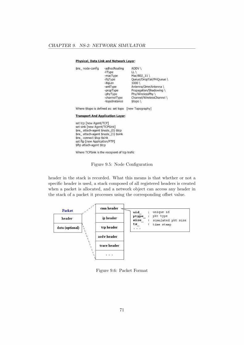
CHAPTER 9. NS-2: NETWORK SIMULATOR
Figure 9.5: Node Configuration
header in the stack is recorded. What this means is that whether or not aspecific header is used, a stack composed of all registered headers is createdwhen a packet is allocated, and a network object can access any header inthe stack of a packet it processes using the corresponding offset value.
Figure 9.6: Packet Format
71

CHAPTER 9. NS-2: NETWORK SIMULATOR
9.2.5 Agent
Agents represent endpoints where network layer packets are generated orconsumed, they implement communication protocols at various layers. Allrouting protocols such as DSDV, DSR and AODV are implemented as agentsbut also the Transport layer protocols TCP and UDP and various applica-tions like CBR (Constant Bit Rate) and FTP (File Transport Protocol).Agents are attached to nodes using the methods shown in figure 9.5.
72

Chapter 10
Simulations
10.1 Configuration
The version of the simulator used in this work is ns-2.29 which can be foundat: ”http://www.isi.edu/nsnam/ns/ns-build.html”. An UMTS-FDD (FDD:Frequency Duplex Division) implementation has also been added to the sim-ulator.
Several UMTS modules are available for NS-2, this study uses an im-plementation developed by the Networking Group in the INFOCOM De-partment at the University of Roma ”La Sapienza” which can be found at:”http://net.infocom.uniroma1.it/”.
This module was preferred to EURANE (Enhanced UMTS Radio Ac-cess Network Extensions) developed within the European Commission 5thframework project SEACORN because EURANE doesn’t allow node mobil-ity.
From http://net.infocom.uniroma1.it/downloads/README:
UMTS Modules for NSThese UMTS modules have been developed by Alfredo To-dini and Francesco Vacirca at the INFOCOM department,University of Rome ”La Sapienza”, Rome, Italy.The code began as a modification of the GPRS package byRicha Jain of the Indian Institute of Technology, Bombay,India.
73

CHAPTER 10. SIMULATIONS
The MAC and physical layers have been rewritten fromscratch; the RLC module instead is based on the GPRS code,but it has been extensively modified, both to overcome its de-ficiencies and to make it work according to the 3GPP speci-fications.Some files in the NS-2 distribution have also been modified.As in the GPRS module, it was necessary to add the NOAH(NO Ad-Hoc Routing Agent) routing algorithm.The archive umts.tgz contains all the necessary files for ns2.1b9a. It should be applied to the ns-2.1b9a all-in-one dis-tribution.
10.2 Modifications to NS-2
First of all, since the UMTS module was originally developed for ns version2.1b9a, modifications within the UMTS module were required to install thisextension.
10.2.1 Double Interface Node
Every mobile terminal used in the simulations are capable of communicat-ing with both an UMTS network and an Ad-Hoc network using the 802.11standards. Since this kind of node didn’t exist in ns-2.29 a new type of nodesupporting both interfaces was developed. Figure 10.1 gives a schematicview of the double interface node used in the simulations.
New fields have been added to the node configuration interface to supportthe addition of the 802.11 component. The added fields are: an Ad-Hocrouting agent (AODV in this case), a Link layer, an interface queue, a MAClayer, a Physical layer, a propagation model and a channel.
In the OTcl code of the simulator (ns-lib.tcl), the add-interface methodof a node is called twice, the first call is made with the UMTS interfacecomponents as parameters and the second with the 802.11 interface compo-nents.
10.2.2 Modifications to AODV
AODV has been modified to incorporate the mechanisms described in theGWAODV chapter. The main modifications are in aodv.(cc,h) and thegateway table operations are defined in gateway table.(cc,h). A new headertype was also defined in aodv packet.h to support Gateway Hello-Messages.
74

CHAPTER 10. SIMULATIONS
Fig
ure
10.1
:Sc
hem
atic
ofa
doub
lein
terf
ace
wir
eles
sno
de
75
CHAPTER 10. SIMULATIONS
10.2.3 Modifications to UMTS MAC FDD
The umts mac fdd.cc had to be modified to maintain an associativity levelbetween the NodeB and the UE. This info is then passed to the RLC layerand finally to the NOAH agent.
10.2.4 Modifications to NOAH
This agent (noah.cc) had to be modified in order to support the arrival ofAODV messages and to decide between using the UMTS interface or the802.11 interface for data packets depending on the reception or not of aNodeB’s signal. The associativity level between the NodeB and the UE ispassed from the NOAH agent to the AODV agent to update the node’sgateway table.
10.2.5 Other Modifications
Other files such as rlc.cc or channel.cc have also been modified to adjust tothe new additions. As a general rule, any modification is marked by a startlabel of: //S ADDED BY BAY and an end label of //E ADDED BY BAY.
Data packets forwarded by a gateway UE from the Ad-Hoc network tothe Cellular network bypass the UMTS RLC mechanisms and go straightto the interface queue. The reason for this ”work-around” is that a complexmechanism involving packet sequence numbers is implemented by the RLCand if forwarded data packets were to be processed by the RLC as regu-lar packets originating from the UE, the sequence number count would becorrupted. This would then generate two different packets with the samesequence number which would cause malfunctions in the RLC layer protocol.
10.3 Simulation Configurations
The simulations which have been carried out in this study rely on CBR1 be-tween sources in the Ad-Hoc network and destinations in the wired network.The analyses of the results were focused on the following parameters:
End-to-end delay; the time interval between the moment a packet is sentby the source and the moment it is received by the destination. In thesimulations presented below, the end-to-end delay is not entirely accurate;it represents the time interval between the moment the packet is sent andthe moment it is received by the RLC layer of the NodeB. However, sincethe delay on the wired network is minimal compared to the delay measuredin the Ad-Hoc network, this approximation does not corrupt the results ofthe simulations.
1Constant Bit Rate
76

CHAPTER 10. SIMULATIONS
Packet delivery fraction; the fraction of received packets to sent packets.The number of sent packets includes messages which have been dropped byGWAODV if no gateway route was available. These messages are generatedby the source but never transmitted on the network.
Routing overhead; the amount of control messages sent. The overheadgenerated by this protocol is solely due to Hello-Messages. Since no mod-ifications were made to the time interval between messages, the calculatedoverhead would be the same using AODV rather than GWAODV.
To generate traffic, a tool developed by CMU-Monarch was used. cbr-gen.tcl found in the ”/indep-utils/cmu-scen-gen” folder of the simulator.This traffic generator takes as parameters: the type of traffic needed, thenumber of nodes in the simulation, a seed for the random number generatorused to determine which nodes establish connections and at what time theystart, the maximum number of connections and the packet sending rate.cbrgen.tcl was modified into cbrgen-mod.tcl in order to create connectionsbetween Ad-Hoc and wired nodes instead of ”inter-Ad-Hoc” connections.
For node mobility, the setdest2 utility version 2, developed by U. Michi-gan and located in the same folder has cbrgen.tcl, generated node move-ment. setdest’s parameters are: maximum speed, minimum speed, numberof nodes, pause time, pause type (uniform [0, 2*pause time] or constant),speed type (uniform or normal [min, max]), maximum time, width of spaceand height of space.
10.4 General Performance
To analyze the general performance of this protocol, several test on a 50node topology and with 700s of simulation time, were performed. Everysimulation shared the same mobility scenario generated by setdest3, witha speed between 1m/s and 2m/s, on the same surface of 1500m by 300m.Three different type of traffic scenario were used, one with a maximumnumber of connections of 10, a second with 20 and the last one with 40maximum connections. For each type of traffic scenario, five simulationswere run with a varying packet rate. All simulations used the Shadowingpropagation model with a path loss of 3.5 and a deviation of 4.
Figure 10.2 gives a summary of setdest’s parameters.2setdest implements the Random Way Point algorithm[31]3mob-50.tcl
77

CHAPTER 10. SIMULATIONS
Function Value-M maximum speed 2.0m/s-m minimum speed 1.0m/s-n number of nodes 50-P pause type 2 (uniform)-p pause time 300s-s speed type 1 (uniform)-t maximum time 700s-v version 2 (UM)-x width of space 1500m-y height of space 300m
Figure 10.2: Setdest Parameters
10.4.1 Results
Average End-To-End Delay
Per Maximum Connections:As we can see on figure 10.3 the average end-to-end delay increases as
more connections are established. This is due to the increase in the networktraffic load; nodes have to process more packets and thus packets spend moretime in queues.
Figure 10.3: Average End-To-End Delay per maximum number of connec-tions
78

CHAPTER 10. SIMULATIONS
As a function of time:Figure 10.4 confirms the fact that as more sources begin to transmit
data, the average end-to-end delay increases.
Figure 10.4: Average End-To-End Delay as a function of time
The average end-to-end delay in every simulation is however, well below150ms which is the maximum delay required for an interactive conversation(voice or multi-media). Above 150ms, voice quality drops below PSTN4
quality.
Average Packet Delivery Fraction
In the two figures below, the simulations consisting of maximum 10 connec-tions well surpass the other simulations in terms of average packet deliveryratio. This is due on one part by the fact that, one simulation for maximum10 connections is extremely prolific and on the other hand, scenarios withmaximum 20 connections suffer from two very poor simulations in term ofpacket delivery ratio. The simulations with maximum 40 connections how-ever, seem to stabilize between 10% and 17%.
A possible explanation for this behaviour is that since the first type ofsimulation deals with only a maximum of 10 connections, if one or two active
4Public Switched Telephone Network
79

CHAPTER 10. SIMULATIONS
nodes benefit from long lasting stable routes, they will compensate for theloss suffered by less fortunate mobiles. In a scenario with a maximum of20 connections, if the majority of active nodes are isolated, the amount ofpackets generated and lost will be too much compared to the successfuldeliveries. For the scenarios with maximum 40 connections, the chancesfor all active nodes to be isolated aren’t as high as with a maximum of 20connections and overall a good 10 to 17% of packets are delivered.
The 20 connection scenarios seem to be in a ”dead zone” where thenumber of active nodes is too important for a small number of fortunatenodes to compensate for isolated mobiles and not high enough to prevent amajority of active nodes from being isolated. This however is speculation,further testing is needed to confirm or refute this theory.
Figure 10.5: Average Packet Delivery Fraction per maximum number ofconnections
Average Overhead
The average overhead is close to constant. The reason for this is thatonly Hello and Gateway-Hello control messages are sent is these simula-tions. There are no RREQ, RREP and RERR because we did not consider”inter-Ad-Hoc” communications.
80

CHAPTER 10. SIMULATIONS
Figure 10.6: Average Packet Delivery Fraction as a function of time
As was said earlier, the generated overhead would have been the same ifAODV was used instead of GWAODV for these simulations.
10.5 Different Propagation Models
To fully understand the contrast between an indoor environment and a bestcase scenario (i.e. a desert plane) with regards to radio propagation, thesame simulation configuration using, cbr-40c-3 a traffic scenario, was runusing the Freespace propagation model.
An urban scenario was also run on the same traffic file as above but witha different mobility scenario. The maximum speed was raised to 10m/s toaccount for vehicle movement. The propagation model used is Shadowingbut with a path loss exponent and deviation of 3.
The following figures: 10.8, 10.9 and 10.10 illustrate the results of thethree simulations.
As expected, the packet delivery fraction is the highest using the Freespacemodel. However the end-to-end delay is the smallest in Shadowing (3.5, 4.0)and the worst in Freespace. Since less packets are dropped when searchingfor a gateway (see figure 10.9) using the Freespace model, more packets areprocessed by nodes due to the existence of several gateway routes. Thiscontributes to the increase of the network traffic load and as we have seenearlier this increases end-to-end delay.
81

CHAPTER 10. SIMULATIONS
Figure 10.7: Average Overhead per maximum number of connections
Figure 10.8: Packet Delivery Fraction per Simulation
82

CHAPTER 10. SIMULATIONS
Figure 10.9: Amount of dropped packets due to the lack of gateway routes
Figure 10.10: Average End-To-End Delay per Simulation
83

CHAPTER 10. SIMULATIONS
10.6 Varying Packet Rate
This section will study the impact of an increasing packet rate on the end-to-end delay and the packet delivery fraction. Three simulations were runwith the same mobility scenario and same propagation model on a 50 nodetopology and a maximum of 40 connections. A different traffic scenario wasused for each simulation; one scenario with a 4 packets/sec rate, a secondwith a 7 packets/sec rate and a third with a 10 packets/sec rate.
As expected, since the network traffic load increases with a higher packetsending rate, the average end-to-end delay increases but remains under the150ms mark. The packet delivery fraction decreases since more packets aredropped when no gateway route is present.
Figure 10.11: Average End-To-End Delay per Sending Rate
10.7 Conclusion
The general performance tests show that this protocol is potentially ableto support voice traffic with regards to end-to-end delay. For the packetdelivery fraction, if we consider only the packets sent when a gateway route ispresent in a node’s gateway table, then the percentage is extremely high; forinstance, the average packet delivery fraction for a scenario with maximum
84

CHAPTER 10. SIMULATIONS
Figure 10.12: Packet Delivery Fraction per Sending Rate
40 connections is 62.7954%. However 10 to 17% in an Ad-Hoc infrastructureis not bad. Nevertheless, the routing overhead, is excessive if the majorityof the nodes in the Ad-Hoc network are within reach of a NodeB.
85
Chapter 11
Conclusion and Future Work
The main objective of this study was to develop an original protocol allowingthe extension of a cellular network through an Ad-Hoc network. In order toachieve this, several notions were presented to place this work in its context.
The first chapter of this study focused on the cellular network infras-tructure and its evolution from the late 40s to today’s recent developments.A detailed description of UMTS was given since the simulations carried outmake use of such a network architecture.
Next, the second network infrastructure used in this study was presented:Ad-Hoc networks. This chapter featured a general presentation of MANETsand also an in depth view of the different categories of protocols and theirmechanisms using several examples.
Then, the reasons motivating the interconnection of such networks wereestablished along with the work which has already been done in this field.The main factor driving this study is the unpredictable nature of indoorradio signal propagation which can cause ”dead spots” preventing devicesfrom gaining access to a cellular network.
The personal contribution part of this study started with a detaileddescription of AODV and ABR, the two protocols on which are based thedeveloped protocol: GWAODV.
The hypotheses and assumptions/limitations of this study preceded acomplete description of GWAODV. This routing protocol’s mechanisms wereviewed in detail and illustrated through several figures.
Finally, the network simulator, NS-2, was presented along with the mod-ifications needed for this study. The simulation configurations and resultsended this work by coming to the conclusion that GWAODV could po-tentially support voice traffic when considering end-to-end delay and thatpacket delivery fraction seems to be satisfactory when dealing with Ad-Hocnetworks.
However, more testing is needed to fully understand the impact that
86

CHAPTER 11. CONCLUSION AND FUTURE WORK
this protocol has on these parameters and what effect this would have onreal world traffic. For instance, several simulations need to be run using adifferent metric order when invoking the gateway selection algorithm andanalyze the results; the packet delivery fraction may increase is the priorityis on associativity.
87

Bibliography
[1] Charles E. Perkins and Elizabeth M. Belding-Royer and Samir R. Das.Ad Hoc On-Demand Distance Vector Routing Protocol. In draft-ietf-manet-aodv-13, February 2003
[2] Chai-Keong Toh. Long-lived Ad Hoc Routing based on the Concept ofAssociativity. In draft-ietf-manet-longlived-adhoc-routing-00.txt
[3] The ns Manual (formerly ns Notes and Documentation). Inhttp://www.isi.edu/nsnam/ns/
[4] Andrew S. Tanenbaum. Third-Generation Mobile Phones: Digital Voiceand Data. In Computer Networks, fourth edition, page 166. PrenticeHall PTR, 2003
[5] Gislain Bocq. UMTS Services. In Chapter: UMTS, edition 1.6, page 8,2006
[6] The 3rd Generation Partnership Project Agreement. December 1998.
[7] 3rd Generation Partnership Project. Feasibility study on 3GPP systemto Wireless Local Area Network (WLAN) interworking (Release 6). InTechnical Specification Group Services and System Aspects, October 2003
[8] IEEE 802.11. In http://en.wikipedia.org/wiki/IEEE 802.11
[9] Charles E. Perkins and Pravin Bhagwat. DSDV Routing over a MultihopWireless Network of Mobile Computers. In Ad Hoc Networking, Addison-Wesley, chapter 3, pages 53-74, 2001
[10] Thomas Clausen and Philippe Jacquet. Optimized Link State RoutingProtocol (OLSR). In RFC3626, October 2003
[11] David B. Johnson and David A. Maltz and Yih-Chun Hu. The DynamicSource Routing Protocol for Mobile Ad Hoc Networks (DSR) In TomaszImielinski and Hank Korth, Mobile Computing, volume 353, pages 153-181. Kluwer Academic Publishers, 1996. Chapter 5.
88

BIBLIOGRAPHY
[12] Vincent D. Park and M. Scott Corson. A Highly Adaptive DistributedRouting Algorithm for Mobile Wireless Networks. At IEEE Conferenceon Computer Communications, INFOCOM’97, April 7-11, 1997, Kobe,Japan
[13] Zygmunt J. Haas and Marc R. Pearlman. The Zone Routing Proto-col (ZRP) for Ad Hoc Networks. In haas-draft-ietf-manet-zone-zrp-00,November 1997
[14] Andrew S. Tanenbaum. Radio and Microwave Transmission. In Com-puter Networks, fourth edition, page 103-105. Prentice Hall PTR, 2003
[15] An Introduction To Wireless Communications.http://gk12.harvard.edu/modules/Radio Propagation.doc
[16] Gislain Bocq. Les trajets multiples. In Chapter: Concepts de Propaga-tion, edition 2.6, page 4, 2006
[17] Theodore S. Rappaport. Wireless Communications - Principles & Prac-tice, IEEE Press, 1996, page 130.
[18] The ns Manual (formerly ns Notes and Documentation). Inhttp://www.isi.edu/nsnam/ns/ page 186.
[19] The ns Manual (formerly ns Notes and Documentation). Inhttp://www.isi.edu/nsnam/ns/ page 188.
[20] H. T. Friis. A note on a simple transmission formula. In Proc. IRE, 34,1946.
[21] Hongyi Wu, Chunming Qiao, Swades De, Ozan Tonguz. IntegratedCellular and Ad-Hoc Relaying Systems: iCAR. In IEEE on SelectedAreas in Communications, Vol. 19, No. 10: 2105-2115, October 2001.
[22] H. Luo, R. Ramjee, P. Sinha, L.E. Li and S. Lu. UCAN: A unifiedcellular and Ad-Hoc network architecture. In Proc. MobiCom, San Diego,CA, USA, 2003.
[23] Lorena Senador-Gomez Lazaro. Aspects For The Integration Of Ad-Hoc and Cellular Networks In Indoor Environments. At Universite Librede Bruxelles, 2006
[24] Anand A. Janefalkar, Kaushik Josiam, Dinesh Rajan. Cellular Ad-hocRelay for Emergencies.
[25] Bharat Bhargava, Xiaoxin Wu, Yi Lu, Weichao Wang. IntegratingHeterogeneous Wireless Technologies: A Cellular Aided Mobile Ad hocNetwork (CAMA). Mob. Netw. Appl. 9, 4 (Aug. 2004), 393-408
89

BIBLIOGRAPHY
[26] Jean-Pierre Hubaux, L. Buttyan and S. Capkun. The Quest for Se-curity in Mobile Ad Hoc Networks. In Proceedings of the 2nd ACMinternational Symposium on Mobile Ad Hoc Networking &Amp; Com-puting (Long Beach, CA, USA, October 04 - 05, 2001). MobiHoc ’01.ACM Press, New York, NY, 146-155.
[27] Naouel Ben Salem, Levente Buttyan, Jean-Pierre Hubaux, MarkusJakobsson. A Charging and Rewarding Scheme for Packet Forwardingin Multi-hop Cellular Networks. In Proceedings of the 4th ACM inter-national Symposium on Mobile Ad Hoc Networking &Amp; Computing(Annapolis, Maryland, USA, June 01 - 03, 2003). MobiHoc ’03. ACMPress, New York, NY, 13-24.
[28] Mohan, M. and Joiner, L. L. Solving billing issues in ad hoc net-works. In Proceedings of the 42nd Annual Southeast Regional Conference(Huntsville, Alabama, April 02 - 03, 2004). ACM-SE 42. ACM Press,New York, NY, 31-36.
[29] Standard Deviation. In http://en.wikipedia.org/wiki/Standard deviation
[30] Andrew S. Tanenbaum. Reference Models. In Computer Networks,fourth edition, page 49. Prentice Hall PTR, 2003
[31] The Random Waypoint Model. In http://www.netlab.tkk.fi/ esa/java/rwp/rwp-model.shtml
90