![Comparative Study on Software Testing Strategies Common ... · cycle.[17]. Some of the software errors are functionality errors, communication errors, syntactic errors, calculation](https://static.fdocuments.in/doc/165x107/5f4f33ff6ee4556a4e5daeb4/comparative-study-on-software-testing-strategies-common-cycle17-some-of.jpg)
Roundoff and Truncation Errors - WordPress.com · It is also convenient to relate these errors to...
33
88 4 CHAPTER OBJECTIVES The primary objective of this chapter is to acquaint you with the major sources of errors involved in numerical methods. Specific objectives and topics covered are • Understanding the distinction between accuracy and precision. • Learning how to quantify error. • Learning how error estimates can be used to decide when to terminate an iterative calculation. • Understanding how roundoff errors occur because digital computers have a limited ability to represent numbers. • Understanding why floating-point numbers have limits on their range and precision. • Recognizing that truncation errors occur when exact mathematical formulations are represented by approximations. • Knowing how to use the Taylor series to estimate truncation errors. • Understanding how to write forward, backward, and centered finite-difference approximations of first and second derivatives. • Recognizing that efforts to minimize truncation errors can sometimes increase roundoff errors. YOU’VE GOT A PROBLEM I n Chap. 1, you developed a numerical model for the velocity of a bungee jumper. To solve the problem with a computer, you had to approximate the derivative of velocity with a finite difference. d v dt ∼ = v t = v(t i +1 ) − v(t i ) t i +1 − t i Roundoff and Truncation Errors
Transcript of Roundoff and Truncation Errors - WordPress.com · It is also convenient to relate these errors to...

88
4
CHAPTER OBJECTIVESThe primary objective of this chapter is to acquaint you with the major sources oferrors involved in numerical methods. Specific objectives and topics covered are
• Understanding the distinction between accuracy and precision.• Learning how to quantify error.• Learning how error estimates can be used to decide when to terminate an iterative
calculation.• Understanding how roundoff errors occur because digital computers have a
limited ability to represent numbers.• Understanding why floating-point numbers have limits on their range and
precision.• Recognizing that truncation errors occur when exact mathematical formulations
are represented by approximations.• Knowing how to use the Taylor series to estimate truncation errors.• Understanding how to write forward, backward, and centered finite-difference
approximations of first and second derivatives.• Recognizing that efforts to minimize truncation errors can sometimes increase
roundoff errors.
YOU’VE GOT A PROBLEM
I n Chap. 1, you developed a numerical model for the velocity of a bungee jumper. Tosolve the problem with a computer, you had to approximate the derivative of velocitywith a finite difference.
dv
dt∼= �v
�t= v(ti+1) − v(ti )
ti+1 − ti
Roundoff and Truncation Errors
cha01102_ch04_088-122.qxd 12/17/10 8:00 AM Page 88
Thus, the resulting solution is not exact—that is, it has error.In addition, the computer you use to obtain the solution is also an imperfect tool. Be-
cause it is a digital device, the computer is limited in its ability to represent the magnitudesand precision of numbers. Consequently, the machine itself yields results that contain error.
So both your mathematical approximation and your digital computer cause your re-sulting model prediction to be uncertain. Your problem is: How do you deal with such un-certainty? In particular, is it possible to understand, quantify and control such errors inorder to obtain acceptable results? This chapter introduces you to some approaches andconcepts that engineers and scientists use to deal with this dilemma.
4.1 ERRORS
Engineers and scientists constantly find themselves having to accomplish objectives basedon uncertain information. Although perfection is a laudable goal, it is rarely if ever at-tained. For example, despite the fact that the model developed from Newton’s second lawis an excellent approximation, it would never in practice exactly predict the jumper’s fall.A variety of factors such as winds and slight variations in air resistance would result in de-viations from the prediction. If these deviations are systematically high or low, then wemight need to develop a new model. However, if they are randomly distributed and tightlygrouped around the prediction, then the deviations might be considered negligible and themodel deemed adequate. Numerical approximations also introduce similar discrepanciesinto the analysis.
This chapter covers basic topics related to the identification, quantification, and mini-mization of these errors. General information concerned with the quantification of error isreviewed in this section. This is followed by Sections 4.2 and 4.3, dealing with the twomajor forms of numerical error: roundoff error (due to computer approximations) and trun-cation error (due to mathematical approximations). We also describe how strategies to re-duce truncation error sometimes increase roundoff. Finally, we briefly discuss errors notdirectly connected with the numerical methods themselves. These include blunders, modelerrors, and data uncertainty.
4.1.1 Accuracy and Precision
The errors associated with both calculations and measurements can be characterized withregard to their accuracy and precision. Accuracy refers to how closely a computed or mea-sured value agrees with the true value. Precision refers to how closely individual computedor measured values agree with each other.
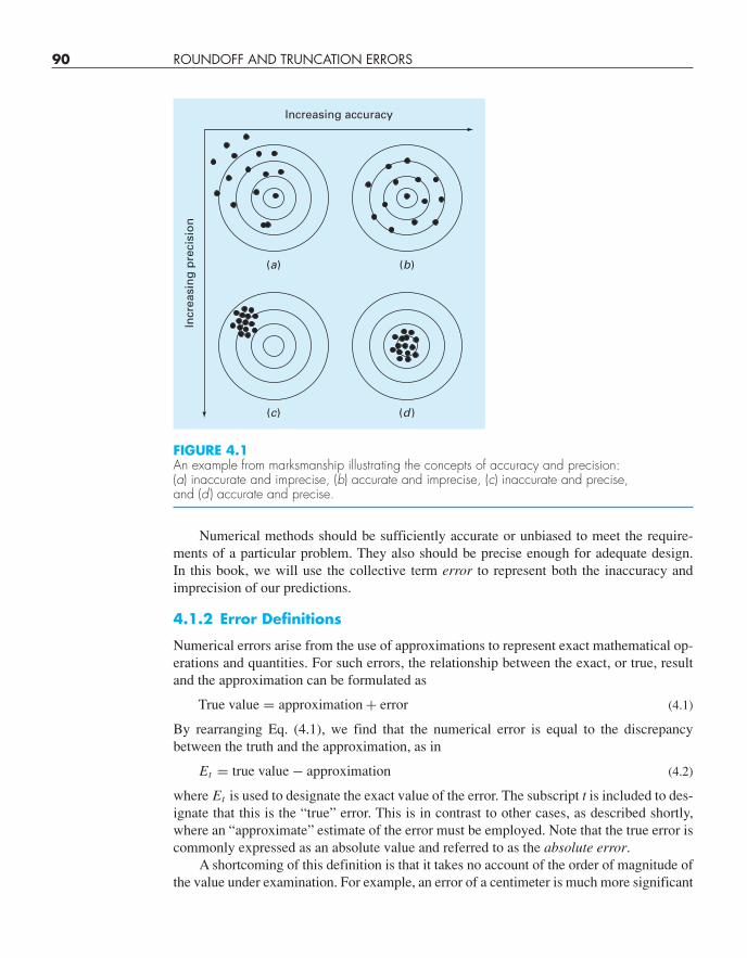
These concepts can be illustrated graphically using an analogy from target practice.The bullet holes on each target in Fig. 4.1 can be thought of as the predictions of a numer-ical technique, whereas the bull’s-eye represents the truth. Inaccuracy (also called bias) isdefined as systematic deviation from the truth. Thus, although the shots in Fig. 4.1c aremore tightly grouped than in Fig. 4.1a, the two cases are equally biased because they areboth centered on the upper left quadrant of the target. Imprecision (also called uncertainty),on the other hand, refers to the magnitude of the scatter. Therefore, although Fig. 4.1b andd are equally accurate (i.e., centered on the bull’s-eye), the latter is more precise becausethe shots are tightly grouped.
4.1 ERRORS 89
cha01102_ch04_088-122.qxd 12/17/10 8:00 AM Page 89
90 ROUNDOFF AND TRUNCATION ERRORS
Numerical methods should be sufficiently accurate or unbiased to meet the require-ments of a particular problem. They also should be precise enough for adequate design.In this book, we will use the collective term error to represent both the inaccuracy andimprecision of our predictions.
4.1.2 Error Definitions
Numerical errors arise from the use of approximations to represent exact mathematical op-erations and quantities. For such errors, the relationship between the exact, or true, resultand the approximation can be formulated as
True value = approximation + error (4.1)
By rearranging Eq. (4.1), we find that the numerical error is equal to the discrepancybetween the truth and the approximation, as in
Et = true value − approximation (4.2)
where Et is used to designate the exact value of the error. The subscript t is included to des-ignate that this is the “true” error. This is in contrast to other cases, as described shortly,where an “approximate” estimate of the error must be employed. Note that the true error iscommonly expressed as an absolute value and referred to as the absolute error.
A shortcoming of this definition is that it takes no account of the order of magnitude ofthe value under examination. For example, an error of a centimeter is much more significant
(c)
(a)
(d )
(b)
Increasing accuracy
Incr
easi
ng
pre
cisi
on
FIGURE 4.1 An example from marksmanship illustrating the concepts of accuracy and precision: (a) inaccurate and imprecise, (b) accurate and imprecise, (c) inaccurate and precise, and (d ) accurate and precise.
cha01102_ch04_088-122.qxd 12/17/10 8:00 AM Page 90
if we are measuring a rivet than a bridge. One way to account for the magnitudes of thequantities being evaluated is to normalize the error to the true value, as in
True fractional relative error = true value − approximation
true value
The relative error can also be multiplied by 100% to express it as
εt = true value − approximation
true value100% (4.3)
where εt designates the true percent relative error.For example, suppose that you have the task of measuring the lengths of a bridge and
a rivet and come up with 9999 and 9 cm, respectively. If the true values are 10,000 and10 cm, respectively, the error in both cases is 1 cm. However, their percent relative errorscan be computed using Eq. (4.3) as 0.01% and 10%, respectively. Thus, although both mea-surements have an absolute error of 1 cm, the relative error for the rivet is much greater. Wewould probably conclude that we have done an adequate job of measuring the bridge,whereas our estimate for the rivet leaves something to be desired.
Notice that for Eqs. (4.2) and (4.3), E and ε are subscripted with a t to signify that theerror is based on the true value. For the example of the rivet and the bridge, we were pro-vided with this value. However, in actual situations such information is rarely available.For numerical methods, the true value will only be known when we deal with functions thatcan be solved analytically. Such will typically be the case when we investigate the theo-retical behavior of a particular technique for simple systems. However, in real-world ap-plications, we will obviously not know the true answer a priori. For these situations, analternative is to normalize the error using the best available estimate of the true value—thatis, to the approximation itself, as in
εa = approximate error
approximation100% (4.4)
where the subscript a signifies that the error is normalized to an approximate value. Notealso that for real-world applications, Eq. (4.2) cannot be used to calculate the error term inthe numerator of Eq. (4.4). One of the challenges of numerical methods is to determineerror estimates in the absence of knowledge regarding the true value. For example, certainnumerical methods use iteration to compute answers. In such cases, a present approxima-tion is made on the basis of a previous approximation. This process is performed repeat-edly, or iteratively, to successively compute (hopefully) better and better approximations.For such cases, the error is often estimated as the difference between the previous and pre-sent approximations. Thus, percent relative error is determined according to
εa = present approximation − previous approximation
present approximation100% (4.5)
This and other approaches for expressing errors is elaborated on in subsequent chapters.The signs of Eqs. (4.2) through (4.5) may be either positive or negative. If the approx-
imation is greater than the true value (or the previous approximation is greater than the cur-rent approximation), the error is negative; if the approximation is less than the true value,the error is positive. Also, for Eqs. (4.3) to (4.5), the denominator may be less than zero,
4.1 ERRORS 91
cha01102_ch04_088-122.qxd 12/17/10 8:00 AM Page 91
92 ROUNDOFF AND TRUNCATION ERRORS
which can also lead to a negative error. Often, when performing computations, we may notbe concerned with the sign of the error but are interested in whether the absolute value of thepercent relative error is lower than a prespecified tolerance εs . Therefore, it is often usefulto employ the absolute value of Eq. (4.5). For such cases, the computation is repeated until
|εa| < εs (4.6)
This relationship is referred to as a stopping criterion. If it is satisfied, our result is assumedto be within the prespecified acceptable level εs . Note that for the remainder of this text, wealmost always employ absolute values when using relative errors.
It is also convenient to relate these errors to the number of significant figures in the ap-proximation. It can be shown (Scarborough, 1966) that if the following criterion is met, wecan be assured that the result is correct to at least n significant figures.
εs = (0.5 × 10²−n)% (4.7)
EXAMPLE 4.1 Error Estimates for Iterative Methods
Problem Statement. In mathematics, functions can often be represented by infinite se-ries. For example, the exponential function can be computed using
ex = 1 + x + x2
2+ x3
3!+ · · · + xn
n!(E4.1.1)
Thus, as more terms are added in sequence, the approximation becomes a better and betterestimate of the true value of ex. Equation (E4.1.1) is called a Maclaurin series expansion.
Starting with the simplest version, ex = 1, add terms one at a time in order to estimatee0.5. After each new term is added, compute the true and approximate percent relative errorswith Eqs. (4.3) and (4.5), respectively. Note that the true value is e0.5 = 1.648721 . . . . Addterms until the absolute value of the approximate error estimate εa falls below a prespeci-fied error criterion εs conforming to three significant figures.
Solution. First, Eq. (4.7) can be employed to determine the error criterion that ensures aresult that is correct to at least three significant figures:
εs = (0.5 × 10²−3)% = 0.05%
Thus, we will add terms to the series until εa falls below this level.The first estimate is simply equal to Eq. (E4.1.1) with a single term. Thus, the first
estimate is equal to 1. The second estimate is then generated by adding the second termas in
ex = 1 + x
or for x = 0.5
e0.5 = 1 + 0.5 = 1.5
This represents a true percent relative error of [Eq. (4.3)]
εt =∣∣∣∣1.648721 − 1.5
1.648721
∣∣∣∣ × 100% = 9.02%
cha01102_ch04_088-122.qxd 12/17/10 8:00 AM Page 92
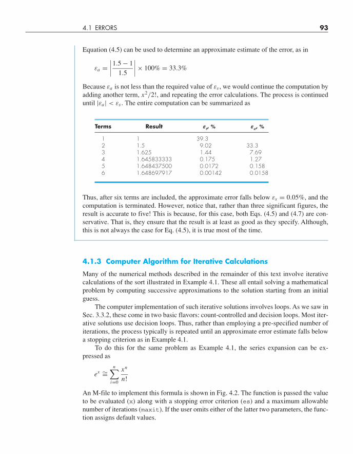
Equation (4.5) can be used to determine an approximate estimate of the error, as in
εa =∣∣∣∣1.5 − 1
1.5
∣∣∣∣ × 100% = 33.3%
Because εa is not less than the required value of εs , we would continue the computation byadding another term, x2/2!, and repeating the error calculations. The process is continueduntil |εa| < εs . The entire computation can be summarized as
Terms Result εt, % εa, %
1 1 39.32 1.5 9.02 33.33 1.625 1.44 7.694 1.645833333 0.175 1.275 1.648437500 0.0172 0.1586 1.648697917 0.00142 0.0158
Thus, after six terms are included, the approximate error falls below εs = 0.05%, and thecomputation is terminated. However, notice that, rather than three significant figures, theresult is accurate to five! This is because, for this case, both Eqs. (4.5) and (4.7) are con-servative. That is, they ensure that the result is at least as good as they specify. Although,this is not always the case for Eq. (4.5), it is true most of the time.
4.1.3 Computer Algorithm for Iterative Calculations
Many of the numerical methods described in the remainder of this text involve iterativecalculations of the sort illustrated in Example 4.1. These all entail solving a mathematicalproblem by computing successive approximations to the solution starting from an initialguess.
The computer implementation of such iterative solutions involves loops. As we saw inSec. 3.3.2, these come in two basic flavors: count-controlled and decision loops. Most iter-ative solutions use decision loops. Thus, rather than employing a pre-specified number ofiterations, the process typically is repeated until an approximate error estimate falls belowa stopping criterion as in Example 4.1.
To do this for the same problem as Example 4.1, the series expansion can be ex-pressed as
ex ∼=n∑
i=0
xn
n!
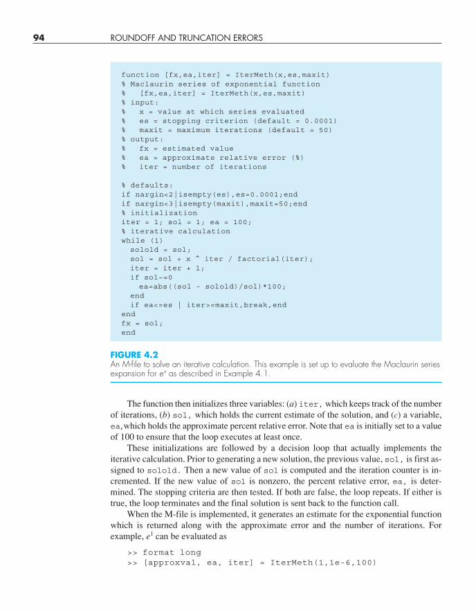
An M-file to implement this formula is shown in Fig. 4.2. The function is passed the valueto be evaluated (x) along with a stopping error criterion (es) and a maximum allowablenumber of iterations (maxit). If the user omits either of the latter two parameters, the func-tion assigns default values.
4.1 ERRORS 93
cha01102_ch04_088-122.qxd 12/17/10 8:00 AM Page 93
94 ROUNDOFF AND TRUNCATION ERRORS
The function then initializes three variables: (a) iter,which keeps track of the numberof iterations, (b) sol, which holds the current estimate of the solution, and (c) a variable,ea,which holds the approximate percent relative error. Note that ea is initially set to a valueof 100 to ensure that the loop executes at least once.
These initializations are followed by a decision loop that actually implements theiterative calculation. Prior to generating a new solution, the previous value, sol, is first as-signed to solold. Then a new value of sol is computed and the iteration counter is in-cremented. If the new value of sol is nonzero, the percent relative error, ea, is deter-mined. The stopping criteria are then tested. If both are false, the loop repeats. If either istrue, the loop terminates and the final solution is sent back to the function call.
When the M-file is implemented, it generates an estimate for the exponential functionwhich is returned along with the approximate error and the number of iterations. Forexample, e1 can be evaluated as
>> format long>> [approxval, ea, iter] = IterMeth(1,1e-6,100)
FIGURE 4.2An M-file to solve an iterative calculation. This example is set up to evaluate the Maclaurin seriesexpansion for ex as described in Example 4.1.
function [fx,ea,iter] = IterMeth(x,es,maxit)% Maclaurin series of exponential function% [fx,ea,iter] = IterMeth(x,es,maxit)% input:% x = value at which series evaluated% es = stopping criterion (default = 0.0001)% maxit = maximum iterations (default = 50)% output:% fx = estimated value% ea = approximate relative error (%)% iter = number of iterations
% defaults:if nargin<2|isempty(es),es=0.0001;endif nargin<3|isempty(maxit),maxit=50;end% initializationiter = 1; sol = 1; ea = 100;% iterative calculationwhile (1)
solold = sol;sol = sol + x ^ iter / factorial(iter);iter = iter + 1;if sol~=0
ea=abs((sol - solold)/sol)*100;endif ea<=es | iter>=maxit,break,end
endfx = sol;end
cha01102_ch04_088-122.qxd 12/17/10 8:00 AM Page 94
approxval =2.718281826198493
ea =9.216155641522974e-007
iter =12
We can see that after 12 iterations, we obtain a result of 2.7182818 with an approximate error estimate of = 9.2162 × 10⁻⁷%. The result can be verified by usingthe built-in exp function to directly calculate the exact value and the true percent rel-ative error,
>> trueval=exp(1)
trueval =2.718281828459046
>> et=abs((trueval- approxval)/trueval)*100
et =8.316108397236229e-008
As was the case with Example 4.1, we obtain the desirable outcome that the true error isless than the approximate error.
4.2 ROUNDOFF ERRORS
Roundoff errors arise because digital computers cannot represent some quantities ex-actly. They are important to engineering and scientific problem solving because theycan lead to erroneous results. In certain cases, they can actually lead to a calculationgoing unstable and yielding obviously erroneous results. Such calculations are said tobe ill-conditioned. Worse still, they can lead to subtler discrepancies that are difficult to detect.
There are two major facets of roundoff errors involved in numerical calculations:
1. Digital computers have magnitude and precision limits on their ability to representnumbers.
2. Certain numerical manipulations are highly sensitive to roundoff errors. This can re-sult from both mathematical considerations as well as from the way in which comput-ers perform arithmetic operations.
4.2.1 Computer Number Representation
Numerical roundoff errors are directly related to the manner in which numbers are storedin a computer. The fundamental unit whereby information is represented is called a word.This is an entity that consists of a string of binary digits, or bits. Numbers are typicallystored in one or more words. To understand how this is accomplished, we must first reviewsome material related to number systems.
A number system is merely a convention for representing quantities. Because we have10 fingers and 10 toes, the number system that we are most familiar with is the decimal, or
4.2 ROUNDOFF ERRORS 95
cha01102_ch04_088-122.qxd 12/17/10 8:00 AM Page 95
96 ROUNDOFF AND TRUNCATION ERRORS
base-10, number system. A base is the number used as the reference for constructing thesystem. The base-10 system uses the 10 digits—0, 1, 2, 3, 4, 5, 6, 7, 8, and 9—to representnumbers. By themselves, these digits are satisfactory for counting from 0 to 9.
For larger quantities, combinations of these basic digits are used, with the position orplace value specifying the magnitude. The rightmost digit in a whole number represents anumber from 0 to 9. The second digit from the right represents a multiple of 10. The thirddigit from the right represents a multiple of 100 and so on. For example, if we have thenumber 8642.9, then we have eight groups of 1000, six groups of 100, four groups of 10,two groups of 1, and nine groups of 0.1, or
(8 × 10³) + (6 × 10²) + (4 × 101) + (2 × 100) + (9 × 10⁻¹) = 8642.9
This type of representation is called positional notation.Now, because the decimal system is so familiar, it is not commonly realized that
there are alternatives. For example, if human beings happened to have eight fingers andtoes we would undoubtedly have developed an octal, or base-8, representation. In thesame sense, our friend the computer is like a two-fingered animal who is limited to twostates—either 0 or 1. This relates to the fact that the primary logic units of digital com-puters are on/off electronic components. Hence, numbers on the computer are repre-sented with a binary, or base-2, system. Just as with the decimal system, quantities can be represented using positional notation. For example, the binary number 101.1 isequivalent to (1 × 22)+ (0 × 21) + (1 × 20) + (1 × 2−1) = 4 + 0 + 1 + 0.5 = 5.5 in the decimal system.
Integer Representation. Now that we have reviewed how base-10 numbers can be rep-resented in binary form, it is simple to conceive of how integers are represented on a com-puter. The most straightforward approach, called the signed magnitude method, employsthe first bit of a word to indicate the sign, with a 0 for positive and a 1 for negative. The re-maining bits are used to store the number. For example, the integer value of 173 is repre-sented in binary as 10101101:
(10101101)2 = 27 + 25 + 23 + 22 + 20 = 128 + 32 + 8 + 4 + 1 = (173)10
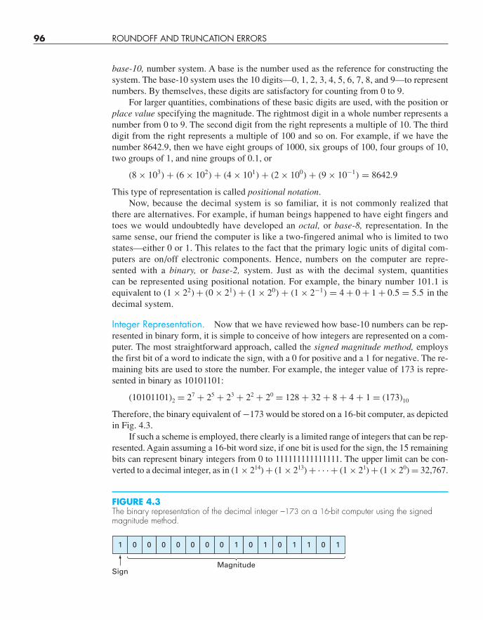
Therefore, the binary equivalent of −173 would be stored on a 16-bit computer, as depictedin Fig. 4.3.
If such a scheme is employed, there clearly is a limited range of integers that can be rep-resented. Again assuming a 16-bit word size, if one bit is used for the sign, the 15 remainingbits can represent binary integers from 0 to 111111111111111. The upper limit can be con-verted to a decimal integer, as in (1 × 214) + (1 × 213) + . . . + (1 × 21) + (1 × 20) = 32,767.
1 0 0 0 0 0 0 0 1 0 1 0 1 1 0 1
SignMagnitude
FIGURE 4.3The binary representation of the decimal integer –173 on a 16-bit computer using the signedmagnitude method.
cha01102_ch04_088-122.qxd 12/17/10 8:00 AM Page 96
Note that this value can be simply evaluated as 215 − 1. Thus, a 16-bit computer word canstore decimal integers ranging from −32,767 to 32,767.
In addition, because zero is already defined as 0000000000000000, it is redundantto use the number 1000000000000000 to define a “minus zero.” Therefore, it is conven-tionally employed to represent an additional negative number: −32,768, and the range isfrom −32,768 to 32,767. For an n-bit word, the range would be from �2n�1 to 2n�1 − 1.Thus, 32-bit integers would range from −2,147,483,648 to +2,147,483,647.
Note that, although it provides a nice way to illustrate our point, the signed magnitudemethod is not actually used to represent integers for conventional computers. A preferredapproach called the 2s complement technique directly incorporates the sign into thenumber’s magnitude rather than providing a separate bit to represent plus or minus.Regardless, the range of numbers is still the same as for the signed magnitude methoddescribed above.
The foregoing serves to illustrate how all digital computers are limited in their capabilityto represent integers. That is, numbers above or below the range cannot be represented. Amore serious limitation is encountered in the storage and manipulation of fractional quanti-ties as described next.
Floating-Point Representation. Fractional quantities are typically represented in com-puters using floating-point format. In this approach, which is very much like scientificnotation, the number is expressed as
±s × be
where s = the significand (or mantissa), b = the base of the number system being used, ande = the exponent.
Prior to being expressed in this form, the number is normalized by moving the decimalplace over so that only one significant digit is to the left of the decimal point. This is done socomputer memory is not wasted on storing useless nonsignificant zeros. For example, a valuelike 0.005678 could be represented in a wasteful manner as 0.005678 × 100. However, nor-malization would yield 5.678 × 10⁻³ which eliminates the useless zeroes.
Before describing the base-2 implementation used on computers, we will first ex-plore the fundamental implications of such floating-point representation. In particular,what are the ramifications of the fact that in order to be stored in the computer, boththe mantissa and the exponent must be limited to a finite number of bits? As in thenext example, a nice way to do this is within the context of our more familiar base-10decimal world.
EXAMPLE 4.2 Implications of Floating-Point Representation
Problem Statement. Suppose that we had a hypothetical base-10 computer with a 5-digitword size. Assume that one digit is used for the sign, two for the exponent, and two for themantissa. For simplicity, assume that one of the exponent digits is used for its sign, leavinga single digit for its magnitude.
Solution. A general representation of the number following normalization would be
s1d1.d2 × 10s0d0
4.2 ROUNDOFF ERRORS 97
cha01102_ch04_088-122.qxd 12/17/10 8:00 AM Page 97
98 ROUNDOFF AND TRUNCATION ERRORS
where s0 and s1 = the signs, d0 = the magnitude of the exponent, and d1 and d2 = the mag-nitude of the significand digits.
Now, let’s play with this system. First, what is the largest possible positive quantitythat can be represented? Clearly, it would correspond to both signs being positive and allmagnitude digits set to the largest possible value in base-10, that is, 9:
Largest value = +9.9 × 10+9
So the largest possible number would be a little less than 10 billion. Although this mightseem like a big number, it’s really not that big. For example, this computer would be inca-pable of representing a commonly used constant like Avogadro’s number (6.022 × 10²³).
In the same sense, the smallest possible positive number would be
Smallest value = +1.0 × 10⁻⁹
Again, although this value might seem pretty small, you could not use it to represent aquantity like Planck’s constant (6.626 × 10⁻³⁴ J ·s).
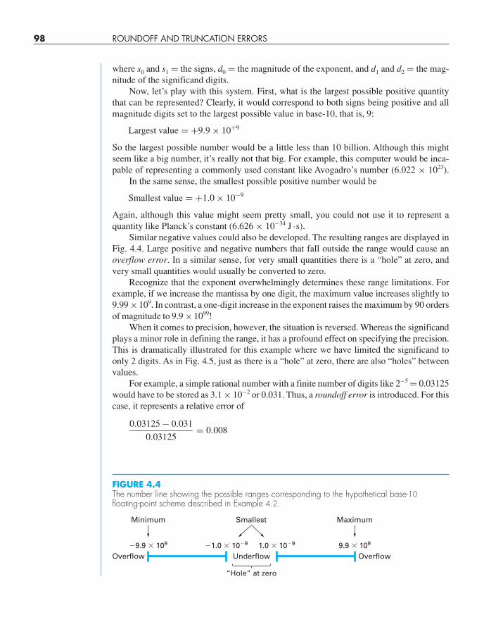
Similar negative values could also be developed. The resulting ranges are displayed inFig. 4.4. Large positive and negative numbers that fall outside the range would cause anoverflow error. In a similar sense, for very small quantities there is a “hole” at zero, andvery small quantities would usually be converted to zero.
Recognize that the exponent overwhelmingly determines these range limitations. Forexample, if we increase the mantissa by one digit, the maximum value increases slightly to9.99 ×109. In contrast, a one-digit increase in the exponent raises the maximum by 90 ordersof magnitude to 9.9 ×1099!
When it comes to precision, however, the situation is reversed. Whereas the significandplays a minor role in defining the range, it has a profound effect on specifying the precision.This is dramatically illustrated for this example where we have limited the significand toonly 2 digits. As in Fig. 4.5, just as there is a “hole” at zero, there are also “holes” betweenvalues.
For example, a simple rational number with a finite number of digits like 2−5 = 0.03125would have to be stored as 3.1 × 10⁻² or 0.031. Thus, a roundoff error is introduced. For thiscase, it represents a relative error of
0.03125 − 0.031
0.03125= 0.008
�9.9 � 109 9.9 � 109�1.0 � 10�9 1.0 � 10�9
“Hole” at zero
SmallestMinimum Maximum
Underflow OverflowOverflow
FIGURE 4.4The number line showing the possible ranges corresponding to the hypothetical base-10floating-point scheme described in Example 4.2.
cha01102_ch04_088-122.qxd 12/17/10 8:00 AM Page 98
While we could store a number like 0.03125 exactly by expanding the digits of thesignificand, quantities with infinite digits must always be approximated. For example, acommonly used constant such as π (= 3.14159…) would have to be represented as 3.1 × 100
or 3.1. For this case, the relative error is
3.14159 − 3.1
3.14159= 0.0132
Although adding significand digits can improve the approximation, such quantities willalways have some roundoff error when stored in a computer.
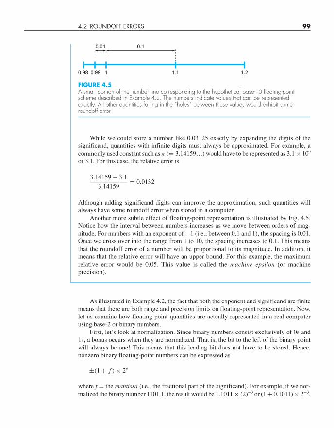
Another more subtle effect of floating-point representation is illustrated by Fig. 4.5.Notice how the interval between numbers increases as we move between orders of mag-nitude. For numbers with an exponent of −1 (i.e., between 0.1 and 1), the spacing is 0.01.Once we cross over into the range from 1 to 10, the spacing increases to 0.1. This meansthat the roundoff error of a number will be proportional to its magnitude. In addition, itmeans that the relative error will have an upper bound. For this example, the maximumrelative error would be 0.05. This value is called the machine epsilon (or machineprecision).
As illustrated in Example 4.2, the fact that both the exponent and significand are finitemeans that there are both range and precision limits on floating-point representation. Now,let us examine how floating-point quantities are actually represented in a real computerusing base-2 or binary numbers.
First, let’s look at normalization. Since binary numbers consist exclusively of 0s and1s, a bonus occurs when they are normalized. That is, the bit to the left of the binary pointwill always be one! This means that this leading bit does not have to be stored. Hence,nonzero binary floating-point numbers can be expressed as
±(1 + f ) × 2e
where f = the mantissa (i.e., the fractional part of the significand). For example, if we nor-malized the binary number 1101.1, the result would be 1.1011 × (2)−3 or (1 + 0.1011) × 2−3.
4.2 ROUNDOFF ERRORS 99
0.98 0.99 1 1.1 1.2
0.01 0.1
FIGURE 4.5A small portion of the number line corresponding to the hypothetical base-10 floating-pointscheme described in Example 4.2. The numbers indicate values that can be represented exactly. All other quantities falling in the “holes” between these values would exhibit someroundoff error.
cha01102_ch04_088-122.qxd 12/17/10 8:00 AM Page 99
100 ROUNDOFF AND TRUNCATION ERRORS
Thus, although the original number has five significant bits, we only have to store the fourfractional bits: 0.1011.
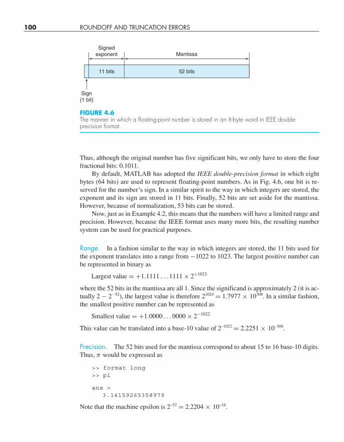
By default, MATLAB has adopted the IEEE double-precision format in which eightbytes (64 bits) are used to represent floating-point numbers. As in Fig. 4.6, one bit is re-served for the number’s sign. In a similar spirit to the way in which integers are stored, theexponent and its sign are stored in 11 bits. Finally, 52 bits are set aside for the mantissa.However, because of normalization, 53 bits can be stored.
Now, just as in Example 4.2, this means that the numbers will have a limited range andprecision. However, because the IEEE format uses many more bits, the resulting numbersystem can be used for practical purposes.
Range. In a fashion similar to the way in which integers are stored, the 11 bits used forthe exponent translates into a range from −1022 to 1023. The largest positive number canbe represented in binary as
Largest value = +1.1111 . . . 1111 × 2+1023
where the 52 bits in the mantissa are all 1. Since the significand is approximately 2 (it is ac-tually 2 − 2−52), the largest value is therefore 21024 = 1.7977 × 10308. In a similar fashion,the smallest positive number can be represented as
Smallest value = +1.0000 . . . 0000 × 2−1022
This value can be translated into a base-10 value of 2–1022 = 2.2251 × 10–308.
Precision. The 52 bits used for the mantissa correspond to about 15 to 16 base-10 digits.Thus, π would be expressed as
>> format long>> pi
ans =3.14159265358979
Note that the machine epsilon is 2–52 = 2.2204 × 10⁻¹⁶.
FIGURE 4.6The manner in which a floating-point number is stored in an 8-byte word in IEEE double-precision format.
Signedexponent
Sign(1 bit)
Mantissa
52 bits11 bits
cha01102_ch04_088-122.qxd 12/17/10 8:00 AM Page 100
MATLAB has a number of built-in functions related to its internal number representa-tion. For example, the realmax function displays the largest positive real number:
>> format long>> realmax
ans =1.797693134862316e+308
Numbers occurring in computations that exceed this value create an overflow. In MATLABthey are set to infinity, inf. The realmin function displays the smallest positive realnumber:
>> realmin
ans =2.225073858507201e-308
Numbers that are smaller than this value create an underflow and, in MATLAB, are set tozero. Finally, the eps function displays the machine epsilon:
>> eps
ans =2.220446049250313e-016
4.2.2 Arithmetic Manipulations of Computer Numbers
Aside from the limitations of a computer’s number system, the actual arithmetic manipula-tions involving these numbers can also result in roundoff error. To understand how thisoccurs, let’s look at how the computer performs simple addition and subtraction.
Because of their familiarity, normalized base-10 numbers will be employed to illus-trate the effect of roundoff errors on simple addition and subtraction. Other number baseswould behave in a similar fashion. To simplify the discussion, we will employ a hypothet-ical decimal computer with a 4-digit mantissa and a 1-digit exponent.
When two floating-point numbers are added, the numbers are first expressed so thatthey have the same exponents. For example, if we want to add 1.557 + 0.04341, the com-puter would express the numbers as 0.1557 × 101 + 0.004341 × 101. Then the mantissasare added to give 0.160041 × 101. Now, because this hypothetical computer only carries a4-digit mantissa, the excess number of digits get chopped off and the result is 0.1600 × 101.Notice how the last two digits of the second number (41) that were shifted to the right haveessentially been lost from the computation.
Subtraction is performed identically to addition except that the sign of the subtrahendis reversed. For example, suppose that we are subtracting 26.86 from 36.41. That is,
0.3641 × 10²
−0.2686 × 10²
0.0955 × 10²
For this case the result must be normalized because the leading zero is unnecessary. Sowe must shift the decimal one place to the right to give 0.9550 × 101 = 9.550. Notice that
4.2 ROUNDOFF ERRORS 101
cha01102_ch04_088-122.qxd 12/17/10 8:00 AM Page 101
102 ROUNDOFF AND TRUNCATION ERRORS
the zero added to the end of the mantissa is not significant but is merely appended to fill theempty space created by the shift. Even more dramatic results would be obtained when thenumbers are very close as in
0.7642 × 10³
−0.7641 × 10³
0.0001 × 10³
which would be converted to 0.1000 × 100 = 0.1000. Thus, for this case, three nonsignif-icant zeros are appended.
The subtracting of two nearly equal numbers is called subtractive cancellation. It isthe classic example of how the manner in which computers handle mathematics can lead tonumerical problems. Other calculations that can cause problems include:
Large Computations. Certain methods require extremely large numbers of arithmeticmanipulations to arrive at their final results. In addition, these computations are often inter-dependent. That is, the later calculations are dependent on the results of earlier ones. Con-sequently, even though an individual roundoff error could be small, the cumulative effectover the course of a large computation can be significant. A very simple case involves sum-ming a round base-10 number that is not round in base-2. Suppose that the following M-fileis constructed:
function sout = sumdemo()s = 0;for i = 1:10000
s = s + 0.0001;endsout = s;
When this function is executed, the result is
>> format long>> sumdemo
ans =0.99999999999991
The format long command lets us see the 15 significant-digit representation usedby MATLAB. You would expect that sum would be equal to 1. However, although0.0001 is a nice round number in base-10, it cannot be expressed exactly in base-2. Thus,the sum comes out to be slightly different than 1. We should note that MATLAB has fea-tures that are designed to minimize such errors. For example, suppose that you form avector as in
>> format long>> s = [0:0.0001:1];
For this case, rather than being equal to 0.99999999999991, the last entry will be exactlyone as verified by
>> s(10001)
ans =1
cha01102_ch04_088-122.qxd 12/17/10 8:00 AM Page 102
Adding a Large and a Small Number. Suppose we add a small number, 0.0010, to alarge number, 4000, using a hypothetical computer with the 4-digit mantissa and the 1-digitexponent. After modifying the smaller number so that its exponent matches the larger,
0.4000 × 10⁴
0.0000001 × 10⁴
0.4000001 × 10⁴
which is chopped to 0.4000 × 10⁴ . Thus, we might as well have not performed the addi-tion! This type of error can occur in the computation of an infinite series. The initial termsin such series are often relatively large in comparison with the later terms. Thus, after a fewterms have been added, we are in the situation of adding a small quantity to a large quan-tity. One way to mitigate this type of error is to sum the series in reverse order. In this way,each new term will be of comparable magnitude to the accumulated sum.
Smearing. Smearing occurs whenever the individual terms in a summation are largerthan the summation itself. One case where this occurs is in a series of mixed signs.
Inner Products. As should be clear from the last sections, some infinite series are partic-ularly prone to roundoff error. Fortunately, the calculation of series is not one of the morecommon operations in numerical methods. A far more ubiquitous manipulation is the cal-culation of inner products as in
n∑i=1
xi yi = x1 y1 + x2 y2 + · · · + xn yn
This operation is very common, particularly in the solution of simultaneous linear algebraicequations. Such summations are prone to roundofferror. Consequently, it is often desirable tocompute such summations in double precision as is done automatically in MATLAB.
4.3 TRUNCATION ERRORS
Truncation errors are those that result from using an approximation in place of an exactmathematical procedure. For example, in Chap. 1 we approximated the derivative of veloc-ity of a bungee jumper by a finite-difference equation of the form [Eq. (1.11)]
dv
dt∼= �v
�t= v(ti+1) − v(ti )
ti+1 − ti(4.8)
A truncation error was introduced into the numerical solution because the difference equa-tion only approximates the true value of the derivative (recall Fig. 1.3). To gain insight intothe properties of such errors, we now turn to a mathematical formulation that is used widelyin numerical methods to express functions in an approximate fashion—the Taylor series.
4.3.1 The Taylor Series
Taylor’s theorem and its associated formula, the Taylor series, is of great value in the studyof numerical methods. In essence, the Taylor theorem states that any smooth function canbe approximated as a polynomial. The Taylor series then provides a means to express thisidea mathematically in a form that can be used to generate practical results.
4.3 TRUNCATION ERRORS 103
cha01102_ch04_088-122.qxd 12/17/10 8:00 AM Page 103
104 ROUNDOFF AND TRUNCATION ERRORS
A useful way to gain insight into the Taylor series is to build it term by term. A goodproblem context for this exercise is to predict a function value at one point in terms of thefunction value and its derivatives at another point.
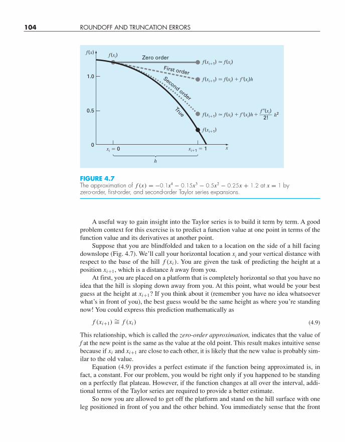
Suppose that you are blindfolded and taken to a location on the side of a hill facingdownslope (Fig. 4.7). We’ll call your horizontal location xi and your vertical distance withrespect to the base of the hill f (xi ). You are given the task of predicting the height at aposition xi+1, which is a distance h away from you.
At first, you are placed on a platform that is completely horizontal so that you have noidea that the hill is sloping down away from you. At this point, what would be your bestguess at the height at xi+1? If you think about it (remember you have no idea whatsoeverwhat’s in front of you), the best guess would be the same height as where you’re standingnow! You could express this prediction mathematically as
f (xi+1) ∼= f (xi ) (4.9)
This relationship, which is called the zero-order approximation, indicates that the value off at the new point is the same as the value at the old point. This result makes intuitive sensebecause if xi and xi+1 are close to each other, it is likely that the new value is probably sim-ilar to the old value.
Equation (4.9) provides a perfect estimate if the function being approximated is, infact, a constant. For our problem, you would be right only if you happened to be standingon a perfectly flat plateau. However, if the function changes at all over the interval, addi-tional terms of the Taylor series are required to provide a better estimate.
So now you are allowed to get off the platform and stand on the hill surface with oneleg positioned in front of you and the other behind. You immediately sense that the front
1.0
0.5
0
h
Zero orderf (x) f (xi)
xi � 0 xi�1 � 1 x
f (xi�1)
f (xi�1) � f (xi) � f �(xi)h �f ��(xi)
2! h2
f (xi�1) � f (xi) � f �(xi)h
f (xi�1) � f (xi)
Second order
True
First order
FIGURE 4.7The approximation of f (x) = −0.1x4 − 0.15x3 − 0.5x2 − 0.25x + 1.2 at x = 1 by zero-order, first-order, and second-order Taylor series expansions.
cha01102_ch04_088-122.qxd 12/17/10 8:00 AM Page 104
foot is lower than the back foot. In fact, you’re allowed to obtain a quantitative estimate ofthe slope by measuring the difference in elevation and dividing it by the distance betweenyour feet.
With this additional information, you’re clearly in a better position to predict theheight at f (xi+1). In essence, you use the slope estimate to project a straight line out toxi+1. You can express this prediction mathematically by
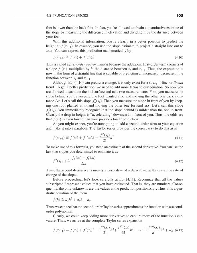
f (xi+1) ∼= f (xi ) + f ′(xi )h (4.10)
This is called a first-order approximation because the additional first-order term consists ofa slope f ′(xi ) multiplied by h, the distance between xi and xi+1. Thus, the expression isnow in the form of a straight line that is capable of predicting an increase or decrease of thefunction between xi and xi+1.
Although Eq. (4.10) can predict a change, it is only exact for a straight-line, or linear,trend. To get a better prediction, we need to add more terms to our equation. So now youare allowed to stand on the hill surface and take two measurements. First, you measure theslope behind you by keeping one foot planted at xi and moving the other one back a dis-tance �x . Let’s call this slope f ′
b(xi ). Then you measure the slope in front of you by keep-ing one foot planted at xi and moving the other one forward �x . Let’s call this slopef ′
f (xi ). You immediately recognize that the slope behind is milder than the one in front.Clearly the drop in height is “accelerating” downward in front of you. Thus, the odds arethat f (xi ) is even lower than your previous linear prediction.
As you might expect, you’re now going to add a second-order term to your equationand make it into a parabola. The Taylor series provides the correct way to do this as in
f (xi+1) ∼= f (xi ) + f ′(xi )h + f ′′(xi )
2!h2 (4.11)
To make use of this formula, you need an estimate of the second derivative. You can use thelast two slopes you determined to estimate it as
f ′′(xi+1) ∼=f ′
f (xi ) − f ′b(xi )
�x(4.12)
Thus, the second derivative is merely a derivative of a derivative; in this case, the rate ofchange of the slope.
Before proceeding, let’s look carefully at Eq. (4.11). Recognize that all the valuessubscripted i represent values that you have estimated. That is, they are numbers. Conse-quently, the only unknowns are the values at the prediction position xi+1. Thus, it is a qua-dratic equation of the form
f (h) ∼= a2h2 + a1h + a0
Thus, we can see that the second-order Taylor series approximates the function with a second-order polynomial.
Clearly, we could keep adding more derivatives to capture more of the function’s cur-vature. Thus, we arrive at the complete Taylor series expansion
f (xi+1) = f (xi ) + f ′(xi )h + f ′′(xi )
2!h2+ f (3)(xi )
3!h3 + · · · + f (n)(xi )
n!hn + Rn (4.13)
4.3 TRUNCATION ERRORS 105
cha01102_ch04_088-122.qxd 12/17/10 8:00 AM Page 105
106 ROUNDOFF AND TRUNCATION ERRORS
Note that because Eq. (4.13) is an infinite series, an equal sign replaces the approximatesign that was used in Eqs. (4.9) through (4.11). A remainder term is also included toaccount for all terms from n + 1 to infinity:
Rn = f (n+1)(ξ)
(n + 1)!hn+1 (4.14)
where the subscript n connotes that this is the remainder for the nth-order approximationand ξ is a value of x that lies somewhere between xi and xi+1.
We can now see why the Taylor theorem states that any smooth function can be ap-proximated as a polynomial and that the Taylor series provides a means to express this ideamathematically.
In general, the nth-order Taylor series expansion will be exact for an nth-order poly-nomial. For other differentiable and continuous functions, such as exponentials and sinu-soids, a finite number of terms will not yield an exact estimate. Each additional term willcontribute some improvement, however slight, to the approximation. This behavior will bedemonstrated in Example 4.3. Only if an infinite number of terms are added will the seriesyield an exact result.
Although the foregoing is true, the practical value of Taylor series expansions is that,in most cases, the inclusion of only a few terms will result in an approximation that is closeenough to the true value for practical purposes. The assessment of how many terms arerequired to get “close enough” is based on the remainder term of the expansion (Eq. 4.14).This relationship has two major drawbacks. First, ξ is not known exactly but merely liessomewhere between xi and xi+1. Second, to evaluate Eq. (4.14), we need to determine the(n + 1)th derivative of f (x). To do this, we need to know f (x). However, if we knewf (x), there would be no need to perform the Taylor series expansion in the presentcontext!
Despite this dilemma, Eq. (4.14) is still useful for gaining insight into truncationerrors. This is because we do have control over the term h in the equation. In other words,we can choose how far away from x we want to evaluate f (x), and we can control the num-ber of terms we include in the expansion. Consequently, Eq. (4.14) is often expressed as
Rn = O(hn+1)
where the nomenclature O(hn+1) means that the truncation error is of the order of hn+1.That is, the error is proportional to the step size h raised to the (n + 1)th power. Althoughthis approximation implies nothing regarding the magnitude of the derivatives that multi-ply hn+1, it is extremely useful in judging the comparative error of numerical methodsbased on Taylor series expansions. For example, if the error is O(h), halving the step sizewill halve the error. On the other hand, if the error is O(h2), halving the step size will quar-ter the error.
In general, we can usually assume that the truncation error is decreased by the additionof terms to the Taylor series. In many cases, if h is sufficiently small, the first- and otherlower-order terms usually account for a disproportionately high percent of the error. Thus,only a few terms are required to obtain an adequate approximation. This property is illus-trated by the following example.
cha01102_ch04_088-122.qxd 12/17/10 8:00 AM Page 106
EXAMPLE 4.3 Approximation of a Function with a Taylor Series Expansion
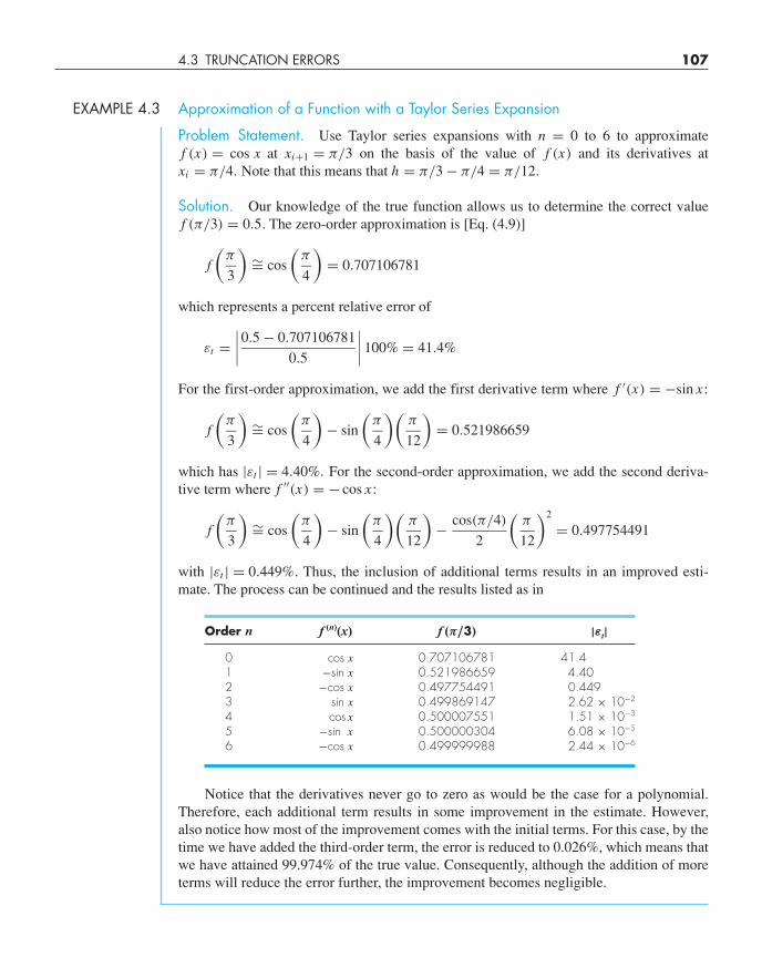
Problem Statement. Use Taylor series expansions with n = 0 to 6 to approximatef (x) = cos x at xi+1 = π/3 on the basis of the value of f (x) and its derivatives atxi = π/4. Note that this means that h = π/3 − π/4 = π/12.
Solution. Our knowledge of the true function allows us to determine the correct valuef (π/3) = 0.5. The zero-order approximation is [Eq. (4.9)]
f
(π
3
)∼= cos
(π
4
)= 0.707106781
which represents a percent relative error of
εt =∣∣∣∣0.5 − 0.707106781
0.5
∣∣∣∣ 100% = 41.4%
For the first-order approximation, we add the first derivative term where f ′(x) = −sin x :
f
(π
3
)∼= cos
(π
4
)− sin
(π
4
)(π
12
)= 0.521986659
which has |εt | = 4.40%. For the second-order approximation, we add the second deriva-tive term where f ′′(x) = − cos x :
f
(π
3
)∼= cos
(π
4
)− sin
(π
4
)(π
12
)− cos(π/4)
2
(π
12
)2
= 0.497754491
with |εt | = 0.449%. Thus, the inclusion of additional terms results in an improved esti-mate. The process can be continued and the results listed as in
Order n f (n)(x) f (π/3) |εt|0 cos x 0.707106781 41.41 −sin x 0.521986659 4.402 −cos x 0.497754491 0.4493 sin x 0.499869147 2.62 × 10⁻²
4 cos x 0.500007551 1.51 × 10⁻³
5 −sin x 0.500000304 6.08 × 10⁻⁵
6 −cos x 0.499999988 2.44 × 10⁻⁶
Notice that the derivatives never go to zero as would be the case for a polynomial.Therefore, each additional term results in some improvement in the estimate. However,also notice how most of the improvement comes with the initial terms. For this case, by thetime we have added the third-order term, the error is reduced to 0.026%, which means thatwe have attained 99.974% of the true value. Consequently, although the addition of moreterms will reduce the error further, the improvement becomes negligible.
4.3 TRUNCATION ERRORS 107
cha01102_ch04_088-122.qxd 12/17/10 8:00 AM Page 107
108 ROUNDOFF AND TRUNCATION ERRORS
4.3.2 The Remainder for the Taylor Series Expansion
Before demonstrating how the Taylor series is actually used to estimate numerical errors,we must explain why we included the argument ξ in Eq. (4.14). To do this, we will use asimple, visually based explanation.
Suppose that we truncated the Taylor series expansion [Eq. (4.13)] after the zero-orderterm to yield
f (xi+1) ∼= f (xi )
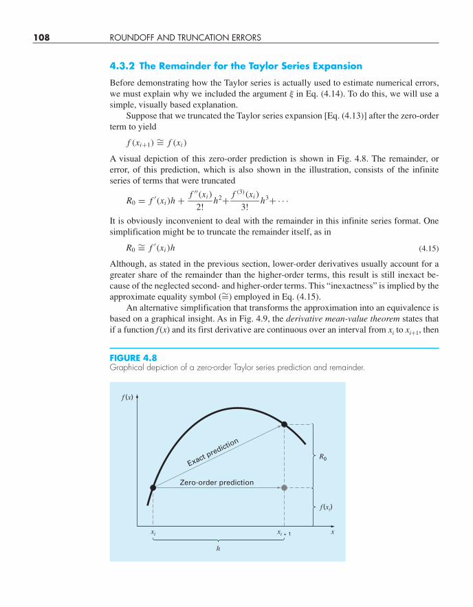
A visual depiction of this zero-order prediction is shown in Fig. 4.8. The remainder, orerror, of this prediction, which is also shown in the illustration, consists of the infiniteseries of terms that were truncated
R0 = f ′(xi )h + f ′′(xi )
2!h2+ f (3)(xi )
3!h3+ · · ·
It is obviously inconvenient to deal with the remainder in this infinite series format. Onesimplification might be to truncate the remainder itself, as in
R0∼= f ′(xi )h (4.15)
Although, as stated in the previous section, lower-order derivatives usually account for agreater share of the remainder than the higher-order terms, this result is still inexact be-cause of the neglected second- and higher-order terms. This “inexactness” is implied by theapproximate equality symbol (∼=) employed in Eq. (4.15).
An alternative simplification that transforms the approximation into an equivalence isbased on a graphical insight. As in Fig. 4.9, the derivative mean-value theorem states thatif a function f (x) and its first derivative are continuous over an interval from xi to xi+1, then
FIGURE 4.8Graphical depiction of a zero-order Taylor series prediction and remainder.
Zero-order prediction
Exact prediction
f (x)
xi xi + 1 x
h
f (xi)
R0
cha01102_ch04_088-122.qxd 12/17/10 8:00 AM Page 108
4.3 TRUNCATION ERRORS 109
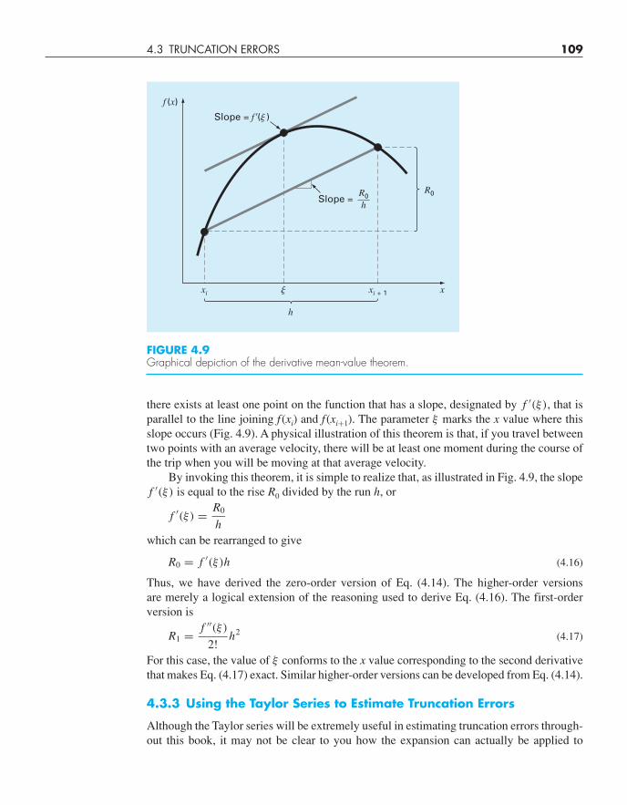
FIGURE 4.9Graphical depiction of the derivative mean-value theorem.
f (x)
xi xi + 1� x
h
R0
Slope = f �(� )
Slope =R0h
there exists at least one point on the function that has a slope, designated by f ′(ξ), that isparallel to the line joining f (xi) and f (xi+1). The parameter ξ marks the x value where thisslope occurs (Fig. 4.9). A physical illustration of this theorem is that, if you travel betweentwo points with an average velocity, there will be at least one moment during the course ofthe trip when you will be moving at that average velocity.
By invoking this theorem, it is simple to realize that, as illustrated in Fig. 4.9, the slopef ′(ξ) is equal to the rise R0 divided by the run h, or
f ′(ξ) = R0
hwhich can be rearranged to give
R0 = f ′(ξ)h (4.16)
Thus, we have derived the zero-order version of Eq. (4.14). The higher-order versionsare merely a logical extension of the reasoning used to derive Eq. (4.16). The first-orderversion is
R1 = f ′′(ξ)
2!h2 (4.17)
For this case, the value of ξ conforms to the x value corresponding to the second derivativethat makes Eq. (4.17) exact. Similar higher-order versions can be developed from Eq. (4.14).
4.3.3 Using the Taylor Series to Estimate Truncation Errors
Although the Taylor series will be extremely useful in estimating truncation errors through-out this book, it may not be clear to you how the expansion can actually be applied to
cha01102_ch04_088-122.qxd 12/17/10 8:00 AM Page 109
110 ROUNDOFF AND TRUNCATION ERRORS
numerical methods. In fact, we have already done so in our example of the bungee jumper.Recall that the objective of both Examples 1.1 and 1.2 was to predict velocity as a functionof time. That is, we were interested in determining v(t). As specified by Eq. (4.13), v(t)can be expanded in a Taylor series:
v(ti+1) = v(ti ) + v′(ti )(ti+1 − ti ) + v′′(ti )2!
(ti+1 − ti )2 + · · · + Rn
Now let us truncate the series after the first derivative term:
v(ti+1) = v(ti ) + v′(ti )(ti+1 − ti ) + R1 (4.18)
Equation (4.18) can be solved for
v′(ti ) = v(ti+1) − v(ti )
ti+1 − ti︸ ︷︷ ︸First order
approximation
− R1
ti+1 − ti︸ ︷︷ ︸Truncation
error
(4.19)
The first part of Eq. (4.19) is exactly the same relationship that was used to approximatethe derivative in Example 1.2 [Eq. (1.11)]. However, because of the Taylor series approach,we have now obtained an estimate of the truncation error associated with this approxima-tion of the derivative. Using Eqs. (4.14) and (4.19) yields
R1
ti+1 − ti= v′′(ξ)
2!(ti+1 − ti )
or
R1
ti+1 − ti= O(ti+1 − ti )
Thus, the estimate of the derivative [Eq. (1.11) or the first part of Eq. (4.19)] has a trunca-tion error of order ti+1 − ti . In other words, the error of our derivative approximationshould be proportional to the step size. Consequently, if we halve the step size, we wouldexpect to halve the error of the derivative.
4.3.4 Numerical Differentiation
Equation (4.19) is given a formal label in numerical methods—it is called a finite differ-ence. It can be represented generally as
f ′(xi ) = f (xi+1) − f (xi )
xi+1 − xi+ O(xi+1 − xi ) (4.20)
or
f ′(xi ) = f (xi+1) − f (xi )
h+ O(h) (4.21)
where h is called the step size—that is, the length of the interval over which the approxi-mation is made, xi+1 − xi . It is termed a “forward” difference because it utilizes data at iand i + 1 to estimate the derivative (Fig. 4.10a).
cha01102_ch04_088-122.qxd 12/17/10 8:00 AM Page 110
4.3 TRUNCATION ERRORS 111
True derivative
True derivative
Approximatio
n
(c)
Approxim
atio
n
(b)
Approximation
(a)
f (x)
f (x)
f (x)
h
xi xxi�1
xi xxi�1
xxi�1 xi�1
h
2h
True derivative
Approximatio
n
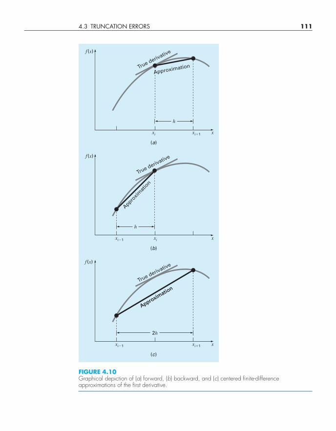
FIGURE 4.10Graphical depiction of (a) forward, (b) backward, and (c) centered finite-differenceapproximations of the first derivative.
cha01102_ch04_088-122.qxd 12/17/10 8:00 AM Page 111
112 ROUNDOFF AND TRUNCATION ERRORS
This forward difference is but one of many that can be developed from the Taylorseries to approximate derivatives numerically. For example, backward and centered differ-ence approximations of the first derivative can be developed in a fashion similar to thederivation of Eq. (4.19). The former utilizes values at xi−1 and xi (Fig. 4.10b), whereasthe latter uses values that are equally spaced around the point at which the derivative isestimated (Fig. 4.10c). More accurate approximations of the first derivative can be devel-oped by including higher-order terms of the Taylor series. Finally, all the foregoing versionscan also be developed for second, third, and higher derivatives. The following sections pro-vide brief summaries illustrating how some of these cases are derived.
Backward Difference Approximation of the First Derivative. The Taylor series can beexpanded backward to calculate a previous value on the basis of a present value, as in
f (xi−1) = f (xi ) − f ′(xi )h + f ′′(xi )
2!h2 − · · · (4.22)
Truncating this equation after the first derivative and rearranging yields
f ′(xi ) ∼= f (xi ) − f (xi−1)
h(4.23)
where the error is O(h).
Centered Difference Approximation of the First Derivative. A third way to approxi-mate the first derivative is to subtract Eq. (4.22) from the forward Taylor series expansion:
f (xi+1) = f (xi ) + f ′(xi )h + f ′′(xi )
2!h2 + · · · (4.24)
to yield
f (xi+1) = f (xi−1) + 2 f ′(xi )h + 2f (3)(xi )
3!h3 + · · ·
which can be solved for
f ′(xi ) = f (xi+1) − f (xi−1)
2h− f (3)(xi )
6h2 + · · ·
or
f ′(xi ) = f (xi+1) − f (xi−1)
2h− O(h2) (4.25)
Equation (4.25) is a centered finite difference representation of the first derivative.Notice that the truncation error is of the order of h2 in contrast to the forward and backwardapproximations that were of the order of h. Consequently, the Taylor series analysis yieldsthe practical information that the centered difference is a more accurate representation ofthe derivative (Fig. 4.10c). For example, if we halve the step size using a forward or back-ward difference, we would approximately halve the truncation error, whereas for the cen-tral difference, the error would be quartered.
cha01102_ch04_088-122.qxd 12/17/10 8:00 AM Page 112
4.3 TRUNCATION ERRORS 113
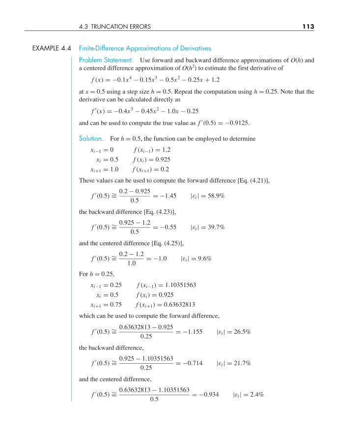
EXAMPLE 4.4 Finite-Difference Approximations of Derivatives
Problem Statement. Use forward and backward difference approximations of O(h) anda centered difference approximation of O(h2) to estimate the first derivative of
f (x) = −0.1x4 − 0.15x3 − 0.5x2 − 0.25x + 1.2
at x = 0.5 using a step size h = 0.5. Repeat the computation using h = 0.25. Note that thederivative can be calculated directly as
f ′(x) = −0.4x3 − 0.45x2 − 1.0x − 0.25
and can be used to compute the true value as f ′(0.5) = −0.9125.
Solution. For h = 0.5, the function can be employed to determine
xi−1 = 0 f (xi−1) = 1.2
xi = 0.5 f (xi ) = 0.925
xi+1 = 1.0 f (xi+1) = 0.2
These values can be used to compute the forward difference [Eq. (4.21)],
f ′(0.5) ∼= 0.2 − 0.925
0.5= −1.45 |εt | = 58.9%
the backward difference [Eq. (4.23)],
f ′(0.5) ∼= 0.925 − 1.2
0.5= −0.55 |εt | = 39.7%
and the centered difference [Eq. (4.25)],
f ′(0.5) ∼= 0.2 − 1.2
1.0= −1.0 |εt | = 9.6%
For h = 0.25,
xi−1 = 0.25 f (xi−1) = 1.10351563
xi = 0.5 f (xi ) = 0.925
xi+1 = 0.75 f (xi+1) = 0.63632813
which can be used to compute the forward difference,
f ′(0.5) ∼= 0.63632813 − 0.925
0.25= −1.155 |εt | = 26.5%
the backward difference,
f ′(0.5) ∼= 0.925 − 1.10351563
0.25= −0.714 |εt | = 21.7%
and the centered difference,
f ′(0.5) ∼= 0.63632813 − 1.10351563
0.5= −0.934 |εt | = 2.4%
cha01102_ch04_088-122.qxd 12/17/10 8:00 AM Page 113
114 ROUNDOFF AND TRUNCATION ERRORS
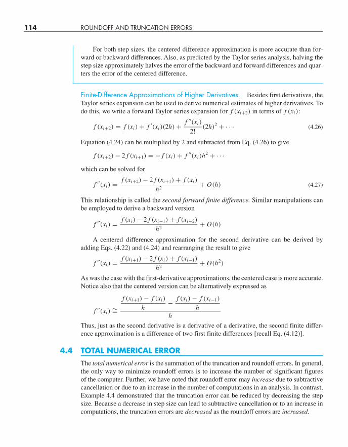
For both step sizes, the centered difference approximation is more accurate than for-ward or backward differences. Also, as predicted by the Taylor series analysis, halving thestep size approximately halves the error of the backward and forward differences and quar-ters the error of the centered difference.
Finite-Difference Approximations of Higher Derivatives. Besides first derivatives, theTaylor series expansion can be used to derive numerical estimates of higher derivatives. Todo this, we write a forward Taylor series expansion for f (xi+2) in terms of f (xi ):
f (xi+2) = f (xi ) + f ′(xi )(2h) + f ′′(xi )
2!(2h)2 + · · · (4.26)
Equation (4.24) can be multiplied by 2 and subtracted from Eq. (4.26) to give
f (xi+2) − 2 f (xi+1) = − f (xi ) + f ′′(xi )h2 + · · ·
which can be solved for
f ′′(xi ) = f (xi+2) − 2 f (xi+1) + f (xi )
h2+ O(h) (4.27)
This relationship is called the second forward finite difference. Similar manipulations canbe employed to derive a backward version
f ′′(xi ) = f (xi ) − 2 f (xi−1) + f (xi−2)
h2+ O(h)
A centered difference approximation for the second derivative can be derived byadding Eqs. (4.22) and (4.24) and rearranging the result to give
f ′′(xi ) = f (xi+1) − 2 f (xi ) + f (xi−1)
h2+ O(h2)
As was the case with the first-derivative approximations, the centered case is more accurate.Notice also that the centered version can be alternatively expressed as
f ′′(xi ) ∼=f (xi+1) − f (xi )
h− f (xi ) − f (xi−1)
hh
Thus, just as the second derivative is a derivative of a derivative, the second finite differ-ence approximation is a difference of two first finite differences [recall Eq. (4.12)].
4.4 TOTAL NUMERICAL ERROR
The total numerical error is the summation of the truncation and roundoff errors. In general,the only way to minimize roundoff errors is to increase the number of significant figuresof the computer. Further, we have noted that roundoff error may increase due to subtractivecancellation or due to an increase in the number of computations in an analysis. In contrast,Example 4.4 demonstrated that the truncation error can be reduced by decreasing the stepsize. Because a decrease in step size can lead to subtractive cancellation or to an increase incomputations, the truncation errors are decreased as the roundoff errors are increased.
cha01102_ch04_088-122.qxd 12/17/10 8:00 AM Page 114
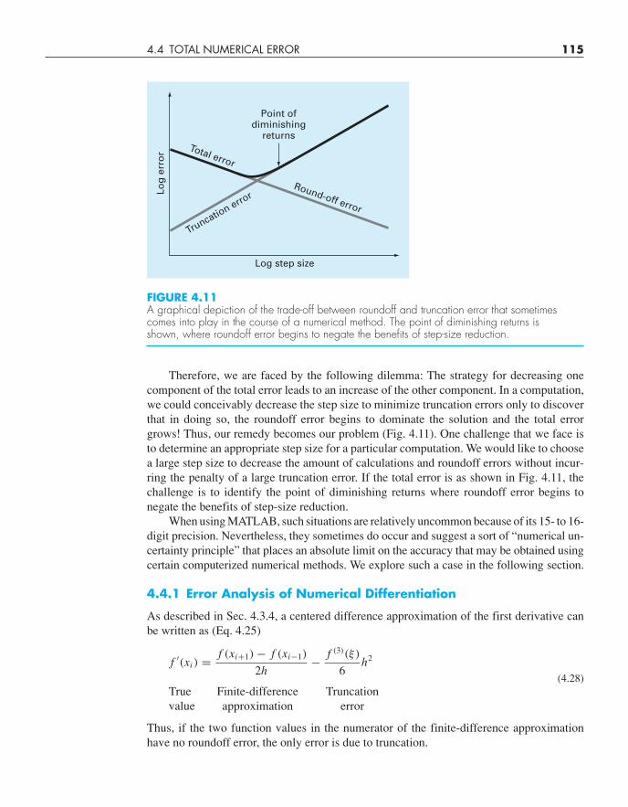
4.4 TOTAL NUMERICAL ERROR 115
Therefore, we are faced by the following dilemma: The strategy for decreasing onecomponent of the total error leads to an increase of the other component. In a computation,we could conceivably decrease the step size to minimize truncation errors only to discoverthat in doing so, the roundoff error begins to dominate the solution and the total errorgrows! Thus, our remedy becomes our problem (Fig. 4.11). One challenge that we face isto determine an appropriate step size for a particular computation. We would like to choosea large step size to decrease the amount of calculations and roundoff errors without incur-ring the penalty of a large truncation error. If the total error is as shown in Fig. 4.11, thechallenge is to identify the point of diminishing returns where roundoff error begins tonegate the benefits of step-size reduction.
When using MATLAB, such situations are relatively uncommon because of its 15- to 16-digit precision. Nevertheless, they sometimes do occur and suggest a sort of “numerical un-certainty principle” that places an absolute limit on the accuracy that may be obtained usingcertain computerized numerical methods. We explore such a case in the following section.
4.4.1 Error Analysis of Numerical Differentiation
As described in Sec. 4.3.4, a centered difference approximation of the first derivative canbe written as (Eq. 4.25)
f ′(xi ) = f (xi+1) − f (xi−1)
2h− f (3)(ξ)
6h2
(4.28)True Finite-difference Truncationvalue approximation error
Thus, if the two function values in the numerator of the finite-difference approximationhave no roundoff error, the only error is due to truncation.
Log step size
Log
err
or
Truncation erro
r
Total error
Point ofdiminishing
returns
Round-off error
FIGURE 4.11A graphical depiction of the trade-off between roundoff and truncation error that sometimescomes into play in the course of a numerical method. The point of diminishing returns is shown, where roundoff error begins to negate the benefits of step-size reduction.
cha01102_ch04_088-122.qxd 12/17/10 8:00 AM Page 115
116 ROUNDOFF AND TRUNCATION ERRORS
However, because we are using digital computers, the function values do includeroundoff error as in
f (xi−1) = f̃ (xi−1) + ei−1
f (xi+1) = f̃ (xi+1) + ei+1
where the f̃ ’s are the rounded function values and the e’s are the associated roundofferrors. Substituting these values into Eq. (4.28) gives
f ′(xi ) = f̃ (xi+1) − f̃ (xi−1)
2h+ ei+1 − ei−1
2h− f (3)(ξ)
6h2
True Finite-difference Roundoff Truncationvalue approximation error error
We can see that the total error of the finite-difference approximation consists of a roundofferror that decreases with step size and a truncation error that increases with step size.
Assuming that the absolute value of each component of the roundoff error has anupper bound of ε, the maximum possible value of the difference ei+1 – ei�1 will be 2ε. Fur-ther, assume that the third derivative has a maximum absolute value of M. An upper boundon the absolute value of the total error can therefore be represented as
Total error =∣∣∣∣∣ f ′(xi ) − f̃ (xi+1) − f̃ (xi−1)
2h
∣∣∣∣∣ ≤ ε
h+ h2 M
6(4.29)
An optimal step size can be determined by differentiating Eq. (4.29), setting the resultequal to zero and solving for
hopt = 3
√3ε
M(4.30)
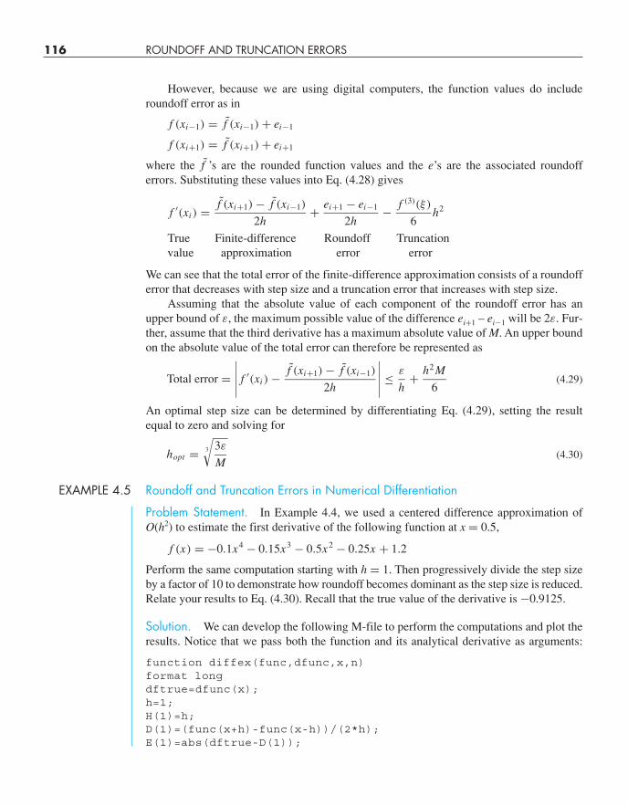
EXAMPLE 4.5 Roundoff and Truncation Errors in Numerical Differentiation
Problem Statement. In Example 4.4, we used a centered difference approximation ofO(h2) to estimate the first derivative of the following function at x = 0.5,
f (x) = −0.1x4 − 0.15x3 − 0.5x2 − 0.25x + 1.2
Perform the same computation starting with h = 1. Then progressively divide the step sizeby a factor of 10 to demonstrate how roundoff becomes dominant as the step size is reduced.Relate your results to Eq. (4.30). Recall that the true value of the derivative is −0.9125.
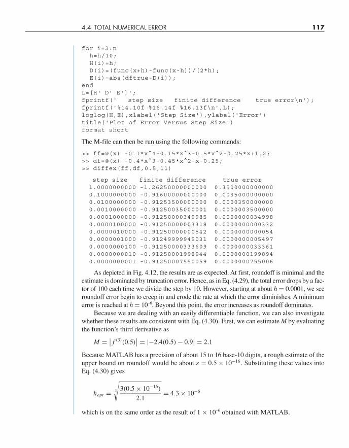
Solution. We can develop the following M-file to perform the computations and plot theresults. Notice that we pass both the function and its analytical derivative as arguments:
function diffex(func,dfunc,x,n)format longdftrue=dfunc(x);h=1;H(1)=h;D(1)=(func(x+h)-func(x-h))/(2*h);E(1)=abs(dftrue-D(1));
cha01102_ch04_088-122.qxd 12/17/10 8:00 AM Page 116
4.4 TOTAL NUMERICAL ERROR 117
for i=2:nh=h/10; H(i)=h;D(i)=(func(x+h)-func(x-h))/(2*h);E(i)=abs(dftrue-D(i));
endL=[H' D' E']';fprintf(' step size finite difference true error\n');fprintf('%14.10f %16.14f %16.13f\n',L);loglog(H,E),xlabel('Step Size'),ylabel('Error')title('Plot of Error Versus Step Size')format short
The M-file can then be run using the following commands:
>> ff=@(x) -0.1*x^4-0.15*x^3-0.5*x^2-0.25*x+1.2;>> df=@(x) -0.4*x^3-0.45*x^2-x-0.25;>> diffex(ff,df,0.5,11)
step size finite difference true error1.0000000000 -1.26250000000000 0.35000000000000.1000000000 -0.91600000000000 0.00350000000000.0100000000 -0.91253500000000 0.00003500000000.0010000000 -0.91250035000001 0.00000035000000.0001000000 -0.91250000349985 0.00000000349980.0000100000 -0.91250000003318 0.00000000003320.0000010000 -0.91250000000542 0.00000000000540.0000001000 -0.91249999945031 0.00000000054970.0000000100 -0.91250000333609 0.00000000333610.0000000010 -0.91250001998944 0.00000001998940.0000000001 -0.91250007550059 0.0000000755006
As depicted in Fig. 4.12, the results are as expected. At first, roundoff is minimal and theestimate is dominated by truncation error. Hence, as in Eq. (4.29), the total error drops by a fac-tor of 100 each time we divide the step by 10. However, starting at about h = 0.0001, we seeroundoff error begin to creep in and erode the rate at which the error diminishes. A minimumerror is reached at h = 10–6. Beyond this point, the error increases as roundoff dominates.
Because we are dealing with an easily differentiable function, we can also investigatewhether these results are consistent with Eq. (4.30). First, we can estimate M by evaluatingthe function’s third derivative as
M = ∣∣ f (3)(0.5)∣∣ = |−2.4(0.5) − 0.9| = 2.1
Because MATLAB has a precision of about 15 to 16 base-10 digits, a rough estimate of theupper bound on roundoff would be about ε = 0.5 × 10⁻¹⁶. Substituting these values intoEq. (4.30) gives
hopt = 3
√3(0.5 × 10⁻¹⁶)
2.1= 4.3 × 10⁻⁶
which is on the same order as the result of 1 × 10⁻⁶ obtained with MATLAB.
cha01102_ch04_088-122.qxd 12/17/10 8:00 AM Page 117
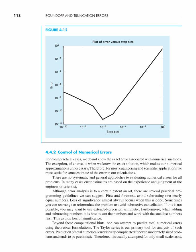
118 ROUNDOFF AND TRUNCATION ERRORS
Plot of error versus step size
100
10�2
10�4
10�6
10�8
10�10
10�12
10�10 10�8 10�6 10�4 10�2 100
Step size
Err
or
FIGURE 4.12
4.4.2 Control of Numerical Errors
For most practical cases, we do not know the exact error associated with numerical methods.The exception, of course, is when we know the exact solution, which makes our numericalapproximations unnecessary. Therefore, for most engineering and scientific applications wemust settle for some estimate of the error in our calculations.
There are no systematic and general approaches to evaluating numerical errors for allproblems. In many cases error estimates are based on the experience and judgment of theengineer or scientist.
Although error analysis is to a certain extent an art, there are several practical pro-gramming guidelines we can suggest. First and foremost, avoid subtracting two nearlyequal numbers. Loss of significance almost always occurs when this is done. Sometimesyou can rearrange or reformulate the problem to avoid subtractive cancellation. If this is notpossible, you may want to use extended-precision arithmetic. Furthermore, when addingand subtracting numbers, it is best to sort the numbers and work with the smallest numbersfirst. This avoids loss of significance.
Beyond these computational hints, one can attempt to predict total numerical errorsusing theoretical formulations. The Taylor series is our primary tool for analysis of sucherrors. Prediction of total numerical error is very complicated for even moderately sized prob-lems and tends to be pessimistic. Therefore, it is usually attempted for only small-scale tasks.
cha01102_ch04_088-122.qxd 12/17/10 8:00 AM Page 118
4.5 BLUNDERS, MODEL ERRORS, AND DATA UNCERTAINTY 119
The tendency is to push forward with the numerical computations and try to estimatethe accuracy of your results. This can sometimes be done by seeing if the results satisfysome condition or equation as a check. Or it may be possible to substitute the results backinto the original equation to check that it is actually satisfied.
Finally you should be prepared to perform numerical experiments to increase yourawareness of computational errors and possible ill-conditioned problems. Such experi-ments may involve repeating the computations with a different step size or method andcomparing the results. We may employ sensitivity analysis to see how our solution changeswhen we change model parameters or input values. We may want to try different numeri-cal algorithms that have different theoretical foundations, are based on different computa-tional strategies, or have different convergence properties and stability characteristics.
When the results of numerical computations are extremely critical and may involveloss of human life or have severe economic ramifications, it is appropriate to take specialprecautions. This may involve the use of two or more independent groups to solve the sameproblem so that their results can be compared.
The roles of errors will be a topic of concern and analysis in all sections of this book.We will leave these investigations to specific sections.
4.5 BLUNDERS, MODEL ERRORS, AND DATA UNCERTAINTY
Although the following sources of error are not directly connected with most of the nu-merical methods in this book, they can sometimes have great impact on the success of amodeling effort. Thus, they must always be kept in mind when applying numerical tech-niques in the context of real-world problems.
4.5.1 Blunders
We are all familiar with gross errors, or blunders. In the early years of computers, erroneousnumerical results could sometimes be attributed to malfunctions of the computer itself.Today, this source of error is highly unlikely, and most blunders must be attributed to humanimperfection.
Blunders can occur at any stage of the mathematical modeling process and can con-tribute to all the other components of error. They can be avoided only by sound knowledgeof fundamental principles and by the care with which you approach and design your solu-tion to a problem.
Blunders are usually disregarded in discussions of numerical methods. This is no doubtdue to the fact that, try as we may, mistakes are to a certain extent unavoidable. However, webelieve that there are a number of ways in which their occurrence can be minimized. In par-ticular, the good programming habits that were outlined in Chap. 3 are extremely useful formitigating programming blunders. In addition, there are usually simple ways to checkwhether a particular numerical method is working properly. Throughout this book, we dis-cuss ways to check the results of numerical calculations.
4.5.2 Model Errors
Model errors relate to bias that can be ascribed to incomplete mathematical models. An ex-ample of a negligible model error is the fact that Newton’s second law does not account forrelativistic effects. This does not detract from the adequacy of the solution in Example 1.1
cha01102_ch04_088-122.qxd 12/17/10 8:00 AM Page 119
120 ROUNDOFF AND TRUNCATION ERRORS
4.1 The “divide and average” method, an old-time methodfor approximating the square root of any positive number a,can be formulated as
x = x + a/x
2
Write a well-structured function to implement this algorithmbased on the algorithm outlined in Fig. 4.2.4.2 Convert the following base-2 numbers to base 10: (a) 1011001, (b) 0.01011, and (c) 110.01001.4.3 Convert the following base-8 numbers to base 10:61,565 and 2.71.4.4 For computers, the machine epsilon ε can also bethought of as the smallest number that when added to one
gives a number greater than 1. An algorithm based on thisidea can be developed as
Step 1: Set ε = 1.Step 2: If 1 + ε is less than or equal to 1, then go to Step 5.
Otherwise go to Step 3.Step 3: ε = ε/2Step 4: Return to Step 2Step 5: ε = 2 × ε
Write your own M-file based on this algorithm to determinethe machine epsilon. Validate the result by comparing it withthe value computed with the built-in function eps.4.5 In a fashion similar to Prob. 4.4, develop your own M-file to determine the smallest positive real number used in
PROBLEMS
because these errors are minimal on the time and space scales associated with the bungeejumper problem.
However, suppose that air resistance is not proportional to the square of the fall velocity,as in Eq. (1.7), but is related to velocity and other factors in a different way. If such were thecase, both the analytical and numerical solutions obtained in Chap. 1 would be erroneous be-cause of model error. You should be cognizant of this type of error and realize that, if you areworking with a poorly conceived model, no numerical method will provide adequate results.
4.5.3 Data Uncertainty
Errors sometimes enter into an analysis because of uncertainty in the physical data on whicha model is based. For instance, suppose we wanted to test the bungee jumper model by hav-ing an individual make repeated jumps and then measuring his or her velocity after a speci-fied time interval. Uncertainty would undoubtedly be associated with these measurements, asthe parachutist would fall faster during some jumps than during others. These errors can ex-hibit both inaccuracy and imprecision. If our instruments consistently underestimate or over-estimate the velocity, we are dealing with an inaccurate, or biased, device. On the other hand,if the measurements are randomly high and low, we are dealing with a question of precision.
Measurement errors can be quantified by summarizing the data with one or more well-chosen statistics that convey as much information as possible regarding specific character-istics of the data. These descriptive statistics are most often selected to represent (1) thelocation of the center of the distribution of the data and (2) the degree of spread of the data.As such, they provide a measure of the bias and imprecision, respectively. We will return tothe topic of characterizing data uncertainty when we discuss regression in Part Four.
Although you must be cognizant of blunders, model errors, and uncertain data, the nu-merical methods used for building models can be studied, for the most part, independentlyof these errors. Therefore, for most of this book, we will assume that we have not made grosserrors, we have a sound model, and we are dealing with error-free measurements. Underthese conditions, we can study numerical errors without complicating factors.
cha01102_ch04_088-122.qxd 12/17/10 8:00 AM Page 120