ROTATION SPACE RANDOM FIELDS WITH AN APPLICATION … · 2017-06-30 · ROTATION SPACE RANDOM FIELDS...
40
The Annals of Statistics 2003, Vol. 31, No. 6, 1732–1771 © Institute of Mathematical Statistics, 2003 ROTATION SPACE RANDOM FIELDS WITH AN APPLICATION TO fMRI DATA 1 BY K. SHAFIE, B. SIGAL, D. SIEGMUND AND K. J. WORSLEY Shahid Beheshti University, Stanford University, Stanford University and McGill University Siegmund and Worsley considered the problem of testing for a signal with unknown location and scale in a Gaussian random field defined on R N . The test statistic was the maximum of a Gaussian random field in an (N + 1)-dimensional “scale space,” N dimensions for location and one dimension for the scale of a smoothing kernel. Siegmund and Worsley used two methods, one involving the expected Euler characteristic of the excursion set and the other involving the volume of tubes, to derive an approximate null distribution. The purpose of this paper is to extend the scale space result to the rotation space random field when N = 2, where the maximum is taken over all rotations of the filter as well as scales. We apply this result to the problem of searching for activation in brain images obtained by functional magnetic resonance imaging (fMRI). 1. Introduction. In a variety of applications in astronomy, neural imaging and genetics, one searches a large space of noisy data for a relatively small number of signals in the form of “bumps” in the random noise. This paper builds on the method suggested by Siegmund and Worsley (1995) to detect such signals, with particular attention to fMRI images. In recent years, very detailed images of the brain, produced by modern sensor technologies, have given the neuroscientist the opportunity to study the functional activation of the brain under different conditions. The main statistical problem is to locate the isolated regions of the brain where activation has occurred (the signal) and separate them from the rest of the brain where no activation can be detected (the noise). To do this, Worsley, Evans, Marrett and Neelin (1992) and Worsley (1994) have shown that the images of the brain can be modeled as a Gaussian random field X(t), where t ∈ R N is a location vector in the brain C ⊂ R N , N = 3. Usually, X max , the global maximum of the random field in C , is chosen as the test statistic for detecting signals in the brain. The images may be spatially smoothed before analysis by convolution with a filter of the form σ −N/2 k(t/σ ) to enhance the signal-to-noise ratio. Often, k(t) is Received November 2000; revised October 2002. 1 Supported by the Natural Sciences and Engineering Research Council of Canada, the Fonds pour la Formation des Chercheurs et l’Aide à la Recherche de Québec and the National Science Foundation. AMS 2000 subject classifications. Primary 60G60, 62M09; secondary 60D05, 52A22. Key words and phrases. Euler characteristic, differential topology, integral geometry, nonstation- ary random fields, image analysis. 1732
Transcript of ROTATION SPACE RANDOM FIELDS WITH AN APPLICATION … · 2017-06-30 · ROTATION SPACE RANDOM FIELDS...

The Annals of Statistics2003, Vol. 31, No. 6, 1732–1771© Institute of Mathematical Statistics, 2003
ROTATION SPACE RANDOM FIELDS WITHAN APPLICATION TO fMRI DATA1
BY K. SHAFIE, B. SIGAL, D. SIEGMUND AND K. J. WORSLEY
Shahid Beheshti University, Stanford University, Stanford Universityand McGill University
Siegmund and Worsley considered the problem of testing for a signalwith unknown location and scale in a Gaussian random field defined on R
N .The test statistic was the maximum of a Gaussian random field in an(N + 1)-dimensional “scale space,” N dimensions for location and onedimension for the scale of a smoothing kernel. Siegmund and Worsley usedtwo methods, one involving the expected Euler characteristic of the excursionset and the other involving the volume of tubes, to derive an approximate nulldistribution. The purpose of this paper is to extend the scale space result to therotation space random field when N = 2, where the maximum is taken overall rotations of the filter as well as scales. We apply this result to the problemof searching for activation in brain images obtained by functional magneticresonance imaging (fMRI).
1. Introduction. In a variety of applications in astronomy, neural imagingand genetics, one searches a large space of noisy data for a relatively small numberof signals in the form of “bumps” in the random noise. This paper builds on themethod suggested by Siegmund and Worsley (1995) to detect such signals, withparticular attention to fMRI images.
In recent years, very detailed images of the brain, produced by modern sensortechnologies, have given the neuroscientist the opportunity to study the functionalactivation of the brain under different conditions. The main statistical problem isto locate the isolated regions of the brain where activation has occurred (the signal)and separate them from the rest of the brain where no activation can be detected(the noise). To do this, Worsley, Evans, Marrett and Neelin (1992) and Worsley(1994) have shown that the images of the brain can be modeled as a Gaussianrandom field X(t), where t ∈ R
N is a location vector in the brain C ⊂ RN , N = 3.
Usually, Xmax, the global maximum of the random field in C, is chosen as the teststatistic for detecting signals in the brain.
The images may be spatially smoothed before analysis by convolution with afilter of the form σ−N/2k(t/σ ) to enhance the signal-to-noise ratio. Often, k(t) is
Received November 2000; revised October 2002.1Supported by the Natural Sciences and Engineering Research Council of Canada, the Fonds
pour la Formation des Chercheurs et l’Aide à la Recherche de Québec and the National ScienceFoundation.
AMS 2000 subject classifications. Primary 60G60, 62M09; secondary 60D05, 52A22.Key words and phrases. Euler characteristic, differential topology, integral geometry, nonstation-
ary random fields, image analysis.
1732

RANDOM FIELDS AND fMRI DATA 1733
proportional to a Gaussian density k(t) ∝ exp(−‖t‖2/2). The motivation for thiscomes from the matched filter theorem of signal processing, which states that asignal added to white noise is best detected by smoothing with a filter whose shapematches that of the signal. A problem is that the scale σ of the signal is usuallyunknown. It is natural to consider searching over filter scale as well as location, thatis, with scale σ varying over a predetermined interval [σ1, σ2]. This adds an extradimension to the search space, called the scale space [see Poline and Mazoyer(1994)]. Siegmund and Worsley (1995) show that Xmax, the global maximumover all locations in C and all scales σ in [σ1, σ2], is the likelihood ratio statisticfor testing for a signal proportional to σ−N/2k(t/σ ) with unknown location andscale. Using two different approaches—(i) the expected Euler characteristic of theexcursion set or (ii) the volume of tubes—they find an approximate P -value of themaximum of the scale space filtered image.
A possible weakness of the scale space random field is a lack of power todetect signals that are not spherically symmetric. In this paper, we extend the scalespace result to rotating filters of the form |S|−1/4k(S−1/2t), where k is sphericallysymmetric and S is now an N × N positive-definite symmetric matrix that rotatesand scales the axes of the filter. Filters of this form add extra dimensions to thesearch space, which we call rotation space. They are expected to have better powerto detect signals that are (approximately) ellipsoidally shaped. A challengingtheoretical problem is to deal adequately with the lack of identifiability of therotation parameter that occurs when the scale parameters are equal.
The concept of scale space has been explored in many image processing tasks[see Lindeberg (1994)] where the filter is usually normalized to preserve the mean;that is, the filter at scale S is |S|−1/2k(S−1/2t). In image processing, there is usuallyno random component, and scale space is used to characterize features in the imagethat are observed without noise. In our case, likelihood principles (see Section 2)dictate that the filter should be normalized to preserve the variance of the filteredwhite-noise background, which leads to a normalization of |S|−1/4 instead.
The normalization used here is the same as that employed by the continuouswavelet transform [Daubechies (1992)], where the filter or mother wavelet isusually chosen so that
∫k(t) dt = 0, as well as
∫k(t)2 dt = 1. The main difference
is that the wavelet transform seeks to represent the image at different scales; herethe aim is to detect a localized image increase at an unknown scale and rotation.
The organization of the paper is as follows. In Section 2, we review the scalespace random field and introduce the rotation space random field. In Section 3,we introduce the Euler characteristic (EC) approach to making inference aboutlocalized signals in these random fields. In Section 4, we introduce a differentparameterization of the rotation space field, which we then study from theviewpoint of the volume of tubes. Approximate P -values obtained by the tubesmethod are shown numerically to be comparable to those obtained by the ECmethod.

1734 SHAFIE, SIGAL, SIEGMUND AND WORSLEY
Although we have used two different methods with two slightly differentparameterizations, there is strong evidence to suggest that these two methodsshould yield the same P -value approximations, at least to the first few terms in thethreshold x. The evidence for this comes from Takemura and Kuriki (2002) whoshow that if the random field has a terminating Karhunen–Loève expansion thenthe EC approach and the tubes approach always give the same answer. In our case(and most interesting cases), the expansion does not terminate, so the agreementbetween the two approaches is still an open question. To illustrate the differentapproaches, we use the EC approach with one parameterization and the tubesmethod with another.
Finally, the power of the rotation space statistic is discussed in Section 5 andis compared to the power of the scale space statistic. In Section 6, we apply therotation space methods to an fMRI data set. Section 7 contains some concludingremarks. Lengthy technical derivations are given in two appendixes.
2. Scale space and rotation space random fields. Let k be an N -dimensionalkernel such that ∫
k2(t) dt = 1.
A common choice is the Gaussian kernel:
k(t) = π−N/4 exp(−‖t‖2/2).(1)
The Gaussian scale space random field is defined as
X(t, σ ) = σ−N/2∫
k[σ−1(h − t)]dZ(h),
where Z(h) is a Gaussian random field defined on a subset of RN and σ is a
positive constant.A justification for working on Gaussian scale space random fields, which also
serves to motivate the rotation space random field of the following section, is asfollows. Assume the random field Z(t), t ∈ R
N , satisfies
dZ(t) = ξσ−N/20 k[σ−1
0 (t − t0)]dt + dW(t),
where t0 ∈ C ⊂ RN , ξ ≥ 0 and σ0 > 0 are fixed values and W is an N -dimensional
Brownian sheet. The unknown parameter (ξ, t0, σ0) represents the amplitude,location and scale of a signal added to the noise dW(t). In other words, the shapeof the signal in dZ(t) matches the shape of the filter k. Models of this form havebeen used in different scientific contexts, for example, in the study of human brainfunction via positron emission tomography [Worsley, Evans, Marrett and Neelin(1992) and Worsley (1994)], in functional magnetic resonance imaging [Worsley(2001)] and for geographical clustering of disease incidences [Rabinowitz (1994)].

RANDOM FIELDS AND fMRI DATA 1735
Now, for testing the hypothesis of no signal, that is, ξ = 0, consider the test statisticthat rejects for large positive values of
Xmax = max(t,σ )∈C×[σ1,σ2]
X(t, σ ).
It can be shown [see Siegmund and Worsley (1995)] that the log-likelihoodfunction is
ξX(t, σ ) − ξ2/2,
so the test defined by Xmax is the likelihood ratio test for testing ξ = 0.We now extend the concept of the scale space random field to the rotation space
random field, which is obtained by rotating as well as scaling the smoothing filter.Using this rotation space random field should increase the sensitivity of the teststatistic in detecting ellipsoidal-shaped signals that might be missed by a circular-shaped filter.
The Gaussian rotation space random field is defined as
X(t,S) = det(S)−1/4∫
k[S−1/2(h − t)]dZ(h),
where k is spherically symmetric and S is an N × N symmetric positive-definitematrix. The same likelihood-based argument as above for working on the scalespace random field justifies working on the rotation space random field. Assumethe random field Z(t), t ∈ R
N , satisfies
dZ(t) = ξ det(S0)−1/4k[S−1/2
0 (t − t0)]dt + dW(t),(2)
where S0 is a member of a fixed parameter set Q of positive-definite matrices. Theunknown parameter (ξ, t0,S0) represents the amplitude, location, orientation andscale of the signal and dW(t) represents noise. The test statistic that rejects forlarge positive values of
Xmax = max(t,S)∈C×Q
X(t,S)
is the likelihood ratio test for testing the hypothesis of no signal, that is, ξ = 0.In this paper, we consider two parameter sets, denoted by Q and Q∗, as search
regions for the 2 × 2 positive-definite matrix S. These are shown schematically inFigure 1. For Q, both eigenvalues are in a fixed interval; for Q∗, one eigenvalue isin a fixed interval, and the ratio of the two eigenvalues is in another fixed interval.As explained in Section 1, we will use two different approaches for the twodifferent parameterizations: the Euler characteristic approach for Q (Section 3)and the tubes approach for Q∗ (Section 4). The choice is arbitrary—we expectboth methods to give very similar results on the same parameterization.

1736 SHAFIE, SIGAL, SIEGMUND AND WORSLEY
FIG. 1. Two-dimensional (N = 2) examples of the two types of rotation space search regionsQ and Q∗ for S shown as contours of the unrotated filter. The axes are the square roots of thetwo eigenvalues l and m of S.
3. The Euler characteristic approach. In this paper, we are primarilyconcerned with finding the P -value of Xmax. A very good approximation is touse the expectation of the EC of the excursion set of the random field inside thesearch region for the maximum [Adler (1981)]. Specifically,
P {Xmax ≥ x} ≈ E[χ(Ax)],where χ denotes the EC and the excursion set Ax is the set of points in thesearch region where the random field exceeds the threshold x. The idea behindthe success of this approach is that for high thresholds the “handles” and “holes”in the excursion set tend to disappear, and the EC counts the number of connectedcomponents of the excursion set. For even higher thresholds, near the maximum,the excursion set contains at most one component, so the EC takes the value 1if the maximum is above x and 0 if it is below. Hence, the expected EC shouldaccurately approximate the probability that the maximum exceeds x. The appeal ofthis approach is that in many cases we can obtain an exact closed-form expressionfor E[χ(Ax)] for all thresholds. Moreover, this closed-form expression typicallygives a very good approximation to the P -value of the maximum for search regionsof almost any size or shape [see Adler (2000)].
There are two main technical challenges to using the EC method. The first isto find a point set representation for the EC using either Morse theory or the

RANDOM FIELDS AND fMRI DATA 1737
Hadwiger recursive definition, so that the EC can be represented as the integralof this point set representation over the interior and boundary of the searchregion. The second step is to evaluate the resulting rather complicated expectationsinvolving the random field and its first two derivatives. The calculations in thissecond step, in the case of the rotation space random field, are so complicated thatwe have used the computer algebra package MAPLE to produce the results [seeShafie (1998) and www.math.mcgill.ca/shafie]. For the scale space random field, ageneral result can be found by hand [Siegmund and Worsley (1995) and Worsley(2001)], and for comparison with the rotation space results yet to come, we nowgive those results.
3.1. Scale space.
3.1.1. Point set representation. The excursion set of the scale space randomfield is
Ax = {(t, σ ) ∈ C × [σ1, σ2] :X(t, σ ) ≥ x
}.
Let Xt = ∂X/∂t, Xt = ∂2X/∂t ∂t′ and c be the inside curvature matrix of ∂C.For a fixed σ , we denote the gradient vector of X in the direction of the insidenormal to ∂C by X⊥ and the gradient (N − 1)-vector in the tangent plane to ∂C
by XT. In addition, let Xσ = ∂X/∂σ and X+σ = Xσ (Xσ > 0). If X(t, σ ) satisfies
the regularity conditions given by Adler (1981), Theorem 5.2.2, then
E[χ(Ax)]=
∫C
∫ σ2
σ1
E[X+σ det(−Xt)|Xt = 0,X = x]φ(0, x) dtdσ
+∫C
[E[(X ≥ x)det(−Xt)|Xt = 0]θ(0)
]σ=σ1
dt(3)
+∫∂C
∫ σ2
σ1
E[X+σ (X⊥ < 0)det(−XT − X⊥c)|XT = 0,X = x]
× φT(0, x) dσ dt
+∫∂C
[E[(X ≥ x)(X⊥ < 0)det(−XT − X⊥c)|XT = 0]θT(0)
]σ=σ1
dt,
where φ(·, ·), θ(·), φT(·, ·) and θT(·) are the densities of (Xt,X), Xt, (XT,X) andXT, respectively.
3.1.2. Expected Euler characteristic. For the second step, Worsley (2001)evaluates this expectation for any number of dimensions N , but for comparisonwith our later rotation space results, we just give the result for N = 2. Letk(h) = ∂k(h)/∂h,
βI =∫
k(h)k′(h) dh, κ =∫
[h′k(h) + (N/2)k(h)]2 dh.

1738 SHAFIE, SIGAL, SIEGMUND AND WORSLEY
For a Gaussian kernel (1), β = 1/2 and κ = N/2. Let r = σ1/σ2, φ(x) =exp(−x2/2)/
√(2π) and (x) = ∫ x
−∞ φ(z) dz. Then
E[χ(Ax)] = |C|βσ−21
{κ1/2(2π)−1/2(1 − r2)(x2 − 1 + 1/κ)/2 + (1 + r2)x/2
}× φ(x)/(2π)
+ |∂C|β1/2σ−11
{κ1/2(2π)−1/2(1 − r)x/2 + (1 + r)/4
}(4)
× φ(x)/(2π)1/2
+ χ(C){[1 − (x)] − κ1/2(2π)−1/2 log rφ(x)
}.
3.2. Rotation space. Turning now to the rotation space random field, we firstdefine the search region. Introducing the rotation filter adds N(N + 1)/2 − 1dimensions to the search space. In general, it is complicated to find the expectationof the EC for such a high-dimensional nonstationary random field, so from nowon we consider the simplest case N = 2. We assume that the rotation parameterS =
(a c
c b
)of the random field is restricted to positive-definite matrices with
eigenvalues limited to the range [σ 21 , σ 2
2 ]. The set Q′ of such matrices, embeddedin R
3, is the union of two cones as shown in Figure 2.To simplify the calculation, we reparameterize Q′ and write
S =[a c
c b
]=
[cos θ − sin θ
sin θ cosθ
][l 00 m
][cosθ sin θ
− sin θ cos θ
],
FIG. 2. Rotation parameter space Q′ for S = [(a, c)′(c, b)′] as the union of two cones with commonaxes along the line a = b (PP). The eigenvalues l and m of S are in the interval [σ 2
1 , σ 22 ]. An example
of the excursion set at a single pixel is added (blob at top right).

RANDOM FIELDS AND fMRI DATA 1739
FIG. 3. Same rotation space as in Figure 2 but reparameterized in terms of eigenvaluesl ≥ m ∈ [σ 2
1 , σ 22 ] and twice the rotation angle ϕ ∈ [0,2π], now denoted by Q. The same example of
the excursion set at a single pixel is added (blob at top right).
where the eigenvalues l and m are in [σ 21 , σ 2
2 ]. Rewriting S in terms of ϕ = 2θ , wehave
S =[
(l + m)/2 + ((l − m)/2) cosϕ ((l − m)/2) sinϕ
((l − m)/2) sinϕ (l + m)/2 − ((l − m)/2) cosϕ
].
In this section, we use s = (l,m,ϕ) instead of S as the parameter of rotation space.Then the domain of the values for s can be considered as
Q = {(l,m,ϕ) :σ 2
1 ≤ m ≤ l ≤ σ 22 , 0 ≤ ϕ ≤ 2π
}.
The set Q is shown in Figure 3. Our aim is to derive E[χ(Ax)], where
Ax = {(t, s) ∈ C × Q :X(t, s) ≥ x
}.
3.2.1. Point set representation. The first step is to find the point set represen-tation for the EC of Ax and take its expectation. As for scale space, we partitionC × Q into different pieces and obtain the contribution of each piece to the EC ofthe excursion set. Then, using the additivity property of the EC and a generalized

1740 SHAFIE, SIGAL, SIEGMUND AND WORSLEY
form of (3), we can obtain the expected EC of the excursion set. In partitioning thesearch set, we face another problem: that the rotation space random field X hassome irregular behavior on P = {(l,m,ϕ) : l = m}. On this set, the random field X
is a constant function of ϕ. Going back to the original rotation space, the union oftwo cones Q′, the set P is the image of P ′, the rotation axis of Q′. The rotationspace random field on this axis is equivalent to a scale space random field. To solvethis irregularity, consider the following. We take away the rotation axis of Q′ andunfold the rest of Q′ to get Q\P and then map the line P ′ to P . Then we considerthe contribution of the image of P ′, P , to the EC of the excursion set separately.The same kind of argument that enables us to separate a part of the search set hasbeen used in the astrophysics literature [see Gott et al. (1990)].
For simplicity in notation, we henceforth denote the set Q\P by Q and proceedby partitioning the rest of the search set as C × Q = (C◦ × Q◦) ∪ (∂C × Q◦) ∪(C × ∂Q) ∪ (∂C × ∂Q), where “◦” denotes the interior of a set. In turn, theboundary of Q itself can be partitioned as
∂Q = B1 ∪ B2 ∪ L ∪ B3 ∪ B4,(5)
where
L = {(l,m,ϕ) : l = σ 2
2 , m = σ 21 , 0 < ϕ < 2π
},
B1 = {(l,m,ϕ) :σ 2
1 ≤ l ≤ σ 22 , m = σ 2
1 , 0 < ϕ < 2π},
B2 = {(l,m,ϕ) : l = σ 2
2 , σ 21 ≤ m ≤ σ 2
2 , 0 < ϕ < 2π},
B3 = {(l,m,ϕ) :σ 2
1 ≤ m ≤ l ≤ σ 22 , ϕ = 0
},
B4 = {(l,m,ϕ) :σ 2
1 ≤ m ≤ l ≤ σ 22 , ϕ = 2π
}.
A diagram of the above partition is shown in Figure 3. We obtain the contributionof P and of each component of the partition of ∂Q in Appendix A.
3.2.2. Expected Euler characteristic. The second step is to evaluate theexpected point set representation just found. To do this, we need to have the jointdistribution of X and its first two derivatives. This distribution can be obtained byusing derivatives of Cov[X(t1,S1),X(t2,S2)]. We have
Cov[X(t1,S1),X(t2,S2)]= det(S1S2)
−1/4∫
k[S−1/21 (h − t1)]k[S−1/2
2 (h − t2)]dh
= det(S1S2)−1/4
∫k[S−1/2
1 (h + t2 − t1)]k[S−1/22 h]dh.
This shows that, for a fixed value of S, X(t,S) is stationary in t, but X(t,S) isnot stationary in (t,S). When k(t) is the Gaussian kernel, the covariance function

RANDOM FIELDS AND fMRI DATA 1741
simplifies to
Cov[X(t1,S1),X(t2,S2)]
= 2N/2 |S1|1/4|S2|1/4
|S1 + S2|1/2exp
(−(t1 − t2)′(S1 + S2)
−1(t1 − t2)/2).
Note that in the case of the Gaussian kernel there are functional relationshipsbetween different derivatives of the rotation space random field X(t,S). Let
XS = ∂X/∂S =[∂X/∂S11 ∂X/∂S12∂X/∂S12 ∂X/∂S22
]
and Xt = ∂2X/∂t ∂t′. Using the heat equation, we can prove that
XS(t,S) = 2N/2−2πN/4(2S−1 − diag(S−1))X(t,S) + Xt(t,S).
As a consequence, it would not be a surprise to see later that some of theconditional distributions are singular.
For simplicity of notation, derivatives of X with respect to ti will be denoted bydot notation with a subscript i, i = 1,2. Derivatives with respect to l, m and ϕ
will be denoted by subscripts l, m and ϕ. To calculate the expectation of theEC, we need to have the distribution of Y = (X, Xϕ, X12lm, X12lm) at a fixedpoint (t, s), where X12lm is arranged in the same way that the vech operatorarranges symmetric matrices [see Searle (1982)]. We know Y has a multivariateGaussian distribution with zero mean. The covariance matrix of Y is obtainedby taking suitable derivatives of Cov[X(t1, s1),X(t2, s2)] then setting t1 = t2 ands1 = s2.
The algebra involved in taking these derivatives for a general kernel is verycomplicated. We decided to choose the Gaussian kernel as the kernel of the rotationspace random field. We used the computer algebra program MAPLE to derive thecovariance matrix for the Gaussian kernel, although our MAPLE code works forany kernel (see www.math.mcgill.ca/shafie). For the Gaussian kernel, we get
Var(Y) =
1 0 0 −Var(X12lm)
0 (l − m)2/(16lm) 0 Cov(Xϕ, X12lm)
0 0 Var(X12lm) Cov(X12lm, X12lm)
−Var(X12lm)′ Cov(Xϕ, X12lm)′ Cov(X12lm, X12lm)′ Var(X12lm)
.
For a detailed evaluation of the elements of Var(Y), see Shafie (1998).Another complication in obtaining the expected EC is the calculation of the
expectation of the determinant of submatrices of X12lm. From Adler (1981),Lemma 5.3.1, it is evident that these expectations depend on the elements of theconditional covariance and mean of X12lm given (X, X). But, unlike the stationarycase, the elements of this covariance matrix are not a symmetric function of theindices (1,2, l,m) [see Adler (1981), page 109]. So to obtain the expectation of therandom determinants, we used MAPLE. The final result is the following theorem.

1742 SHAFIE, SIGAL, SIEGMUND AND WORSLEY
THEOREM 1. For the rotation space random field with a Gaussian kernel, wehave
E[χ(Ax)]
= |C|√
2
σ 21
{−((log r)(1 + r2) + (1 − r2))x4
128π3/2 − (log r)(1 − r2)x3
64π
+ ((2π + 15)(1 − r2) + 7(log r)(1 + r2))x2
128π3/2
+ (2√
2(1 + r2) + 3(log r)(1 − r2))x
32π− (π + 2)(1 − r2)
32π3/2
}φ(x)
+ |∂C| 1
σ1
{∫ (1−r2)1/2
0f (t) dt(6)
+ g +[√
2
8π(r − 1)x + 1
8√
π(r + 1)
]}φ(x)
+ χ(C)
√2
8
{[(2r(log r) − r2 + 1)x2
2√
πr− (2r − r2 − 1)x
r
+ −5r(log r) + (π − 1)(1 − r2)√πr
]φ(x)
+ 1 − (x)
},
where
f (t) =√
2
32π2
{[(t3
t ′3− rt3
t ′4)x3 +
(√πt3
t ′3−
√πrt3
t ′6)x2
+(−8 + 6t2 + 5t4
t ′3t− (8 − 6t2 − 5t4)r
t ′4)x
+ (4 − 2t2 − 3t4)√
π
t ′3t+ (−4 + 6t2 + t4)
√πr
t ′6]E(t)
+[(
−2(4 − t2)r
tt ′+ 2(4 − 5t2 + 2t4)r)
tt ′4)x
− 4√
π
tt ′+ 4
√πr
tt ′2]K(t)
},
g =√
2
32π3/2r
[4r2K[(1 − r2)1/2]− (
(1 − r2)√
πx + 2(1 + r2))E[(1 − r2)1/2]],
RANDOM FIELDS AND fMRI DATA 1743
t ′ = (1 − t2)1/2 and K(·) and E(·) are complete elliptic integrals of the first andsecond kinds, respectively.
The elliptic integrals are defined by K(y) = ∫ π/20 (1 − y2 sin2 θ)−1/2 dθ and
E(y) = ∫ π/20 (1 − y2 sin2 θ)1/2 dθ and are easily evaluated numerically [cf.
Abramowitz and Stegun (1964)]. If only moderate accuracy is required, a simpleapproximation is obtained by expanding the integrands as power series in y andintegrating term by term.
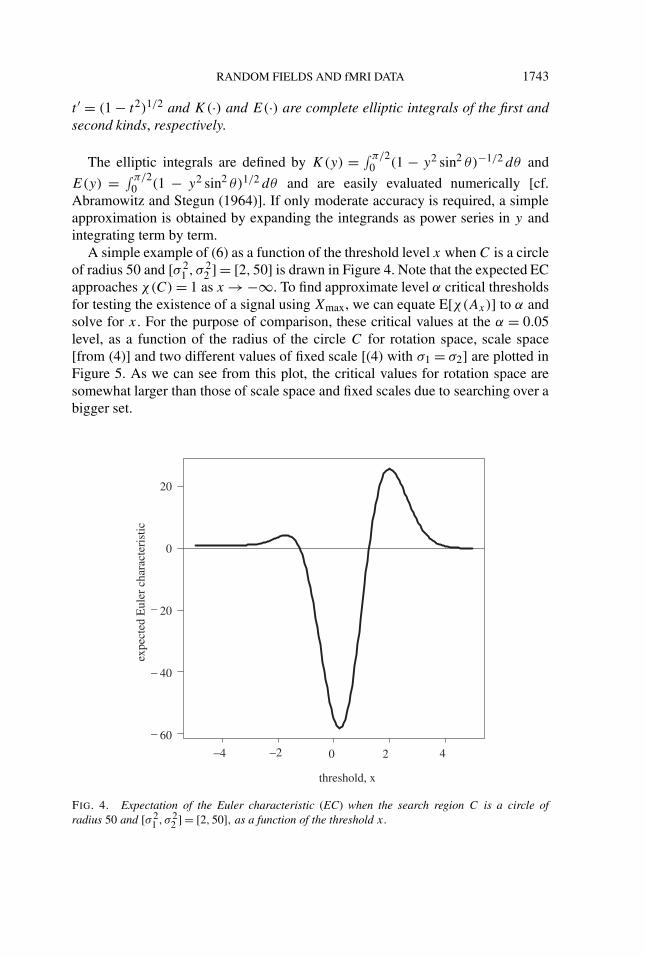
A simple example of (6) as a function of the threshold level x when C is a circleof radius 50 and [σ 2
1 , σ 22 ] = [2,50] is drawn in Figure 4. Note that the expected EC
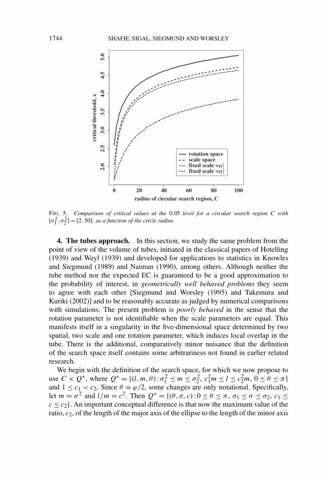
approaches χ(C) = 1 as x → −∞. To find approximate level α critical thresholdsfor testing the existence of a signal using Xmax, we can equate E[χ(Ax)] to α andsolve for x. For the purpose of comparison, these critical values at the α = 0.05level, as a function of the radius of the circle C for rotation space, scale space[from (4)] and two different values of fixed scale [(4) with σ1 = σ2] are plotted inFigure 5. As we can see from this plot, the critical values for rotation space aresomewhat larger than those of scale space and fixed scales due to searching over abigger set.
FIG. 4. Expectation of the Euler characteristic (EC) when the search region C is a circle ofradius 50 and [σ 2
1 , σ 22 ] = [2,50], as a function of the threshold x.
1744 SHAFIE, SIGAL, SIEGMUND AND WORSLEY
FIG. 5. Comparison of critical values at the 0.05 level for a circular search region C with[σ 2
1 , σ 22 ] = [2,50], as a function of the circle radius.
4. The tubes approach. In this section, we study the same problem from thepoint of view of the volume of tubes, initiated in the classical papers of Hotelling(1939) and Weyl (1939) and developed for applications to statistics in Knowlesand Siegmund (1989) and Naiman (1990), among others. Although neither thetube method nor the expected EC is guaranteed to be a good approximation tothe probability of interest, in geometrically well behaved problems they seemto agree with each other [Siegmund and Worsley (1995) and Takemura andKuriki (2002)] and to be reasonably accurate as judged by numerical comparisonswith simulations. The present problem is poorly behaved in the sense that therotation parameter is not identifiable when the scale parameters are equal. Thismanifests itself in a singularity in the five-dimensional space determined by twospatial, two scale and one rotation parameter, which induces local overlap in thetube. There is the additional, comparatively minor nuisance that the definitionof the search space itself contains some arbitrariness not found in earlier relatedresearch.
We begin with the definition of the search space, for which we now propose touse C × Q∗, where Q∗ = {(l,m, θ) :σ 2
1 ≤ m ≤ σ 22 , c2
1m ≤ l ≤ c22m, 0 ≤ θ ≤ π}
and 1 ≤ c1 < c2. Since θ = ϕ/2, some changes are only notational. Specifically,let m = σ 2 and l/m = c2. Then Q∗ = {(θ, σ, c) : 0 ≤ θ ≤ π , σ1 ≤ σ ≤ σ2, c1 ≤c ≤ c2}. An important conceptual difference is that now the maximum value of theratio, c2, of the length of the major axis of the ellipse to the length of the minor axis

RANDOM FIELDS AND fMRI DATA 1745
is the same for all permissible lengths of the minor axis (i.e., the ellipse is no longerrequired to become more circular when the minor axis approaches its maximumpermitted length). Note that if c1 = 1 and c2 = σ2/σ1, then Q∗ contains Q (seeFigure 1). A second important difference is that by explicitly introducing thepossibility that c1 > 1, we are now providing a device to gather some informationabout the singular behavior that occurs at c1 = 1. As a conceptual statistical matter,the first difference seems more important, but the mathematics connected with thesecond difference poses particularly challenging problems. Although this problemdoes not seem to pose a serious impediment to applications, we have not been ableto solve it to our satisfaction. (See the remark at the end of this section.)
Note that if we replace the relations 1 ≤ c1 < c2 by c1 < c2 ≤ 1, while leavingthe constraints on l and m unchanged, or, equivalently, we interchange l and m
while leaving c1 and c2 unchanged, we obtain a different search region. It wouldalso be possible to consider the union of the two search regions, but we have notmade the appropriate calculations.
We recall that the volume-of-tubes viewpoint is based first of all on the possiblyfictitious assumption that the Gaussian field of interest, say X(u), which isstandardized to have mean function 0 and variance function 1 as u runs through anarbitrary indexing set, has a terminating Karhunen–Loève expansion, say X(u) =∑d
1 γi(u)Zi . Here the Zi are independent standard normal random variables, andγ (u) = (γ1(u), . . . , γd(u))′ is a vector of Euclidean norm equal to 1, which asa function of u defines a submanifold � of the unit sphere in d-dimensionalEuclidean space. Since the final approximation depends only on quantities thatcan be calculated from the metric tensor of the manifold, the finiteness of d is notrequired for the approximating expression to make sense. Hence, we can and douse the tubes method whether the assumption of a finite expansion is satisfied ornot. Little is known about the mathematical validity of the approximation whend = ∞ [see, however, Sun (1993)], but simulations show it is quite accurate. SeeAdler (2000) for a more thorough discussion.
Now we give the volume-of-tubes approximation when the kernel k can beexpressed as k(h) = π−1/2g(h′h) for a one-dimensional nonincreasing function g
defined on [0,∞) and satisfying∫∞
0 g(x)2 dx = 1. The associated Gaussian fieldis defined by
X(t,S) = π−1/2 det(S)−1/4∫
R2g[(h − t)′S−1(h − t)]dW(h),
where W is Gaussian white noise and S is a symmetric, positive-definite 2 × 2matrix. With this notation, we can now state our approximation for the generalradial kernel and c1 > 1. The approximation for c2 < 1 is obtained from (8) bychanging the sign of the expression on the right-hand side of (8) and by changingthe elliptic integral E(·) to c−1E[(1 − c2)1/2] each time it appears. For c1 = 1, seebelow.

1746 SHAFIE, SIGAL, SIEGMUND AND WORSLEY
THEOREM 2. For the rotation space random field with a general radial kernel,for each σ1 < σ2 and 1 < c1 < c2, and as x → ∞, we have
P
{max
(t,θ,σ,c)∈C×Q∗ X(t,S) ≥ x
}
≈ φ(x)x4
(2π)5/2
πβ1β2(4β2 − 1)1/2|C|4
(1 − r2)
σ 21
(2 log
c2
c1+ 1
c22
− 1
c21
)
+ φ(x)x3
(2π)2
{π |C|β1[β2(6β2 − 1)]1/2
4√
2
(1 + r2)
σ 21
(2 log
c2
c1+ 1
c22
− 1
c21
)
+ πβ1[β2(4β2 − 1)]1/2|C|2√
2
(1 − r2)
σ 21
(2 − 1
c22
− 1
c21
)
+ β2(β1(4β2 − 1))1/2|∂C|21/2
(1 − r)
σ1
×∫ c2
c1
c2 − 1
c2 E
[(c2 − 1
c2
)1/2]dc
}
+ φ(x)x2
(2π)5/2
{π |C|β1[−6β2(4β2 − 1) − (3β2 − 1)]
4(4β2 − 1)1/2
× (1 − r2)
σ 21
(2 log
c2
c1+ 1
c22
− 1
c21
)(7)
− β2(4β2 − 1)1/2π2χ(C)(log r)
(c2 − c1 + 1
c2− 1
c1
)
+ (β1β2(6β2 − 1))1/2|∂C|π2
(1 + r)
σ1
×∫ c2
c1
c2 − 1
c2 E
[(c2 − 1
c2
)1/2]dc
+ (β1β2(4β2 − 1)
)1/2|∂C|π (1 − r)
σ1
×2∑
i=1
c2i − 1
ci
E
[(c2i − 1
c2i
)1/2]
+ β1(2β2)1/2π |C| 1
σ 21
×(
c21 − 1
c21
(r2 arccosβ3 + (π − arccosβ3)
)
+ c22 − 1
c22
(arccosβ3 + r2(π − arccosβ3)
))},

RANDOM FIELDS AND fMRI DATA 1747
where
β1 =∫ ∞
0g(x)2x dx, β2 =
∫ ∞0
g(x)2x2 dx,
β3 = [(4β2 − 1)/(6β2 − 1)]1/2.
The formula for the Gaussian kernel g(x) = exp(−x/2) can be obtained bytaking β1 = 1/4 and β2 = 1/2.
COROLLARY 1. For the rotation space random field with a Gaussian kernel,we have
P
{max
(t,θ,σ,c)∈C×Q∗ X(t, θ, σ, c) ≥ x
}
≈ φ(x)x4
(2π)5/2
π |C|32
(1 − r2)
σ 21
(2 log
c2
c1+ 1
c22
− 1
c21
)
+ φ(x)x3
(2π)2
{π |C|16
√2
(1 + r2)
σ 21
(2 log
c2
c1+ 1
c22
− 1
c21
)
+ π |C|16
(1 − r2)
σ 21
(2 − 1
c22
− 1
c21
)
+ |∂C|4√
2
(1 − r)
σ1
∫ c2
c1
c2 − 1
c2E
[(c2 − 1
c2
)1/2]dc
}
+ φ(x)x2
(2π)5/2
{(−7)π |C|
32
(1 − r2)
σ 21
(2 log
c2
c1+ 1
c22
− 1
c21
)
− π2χ(C)
2log r
(c2 − c1 + 1
c2− 1
c1
)(8)
+ |∂C|π4
(1 + r)
σ1
∫ c2
c1
c2 − 1
c2E
[(c2 − 1
c2
)1/2]dc
+ |∂C|π2√
2
(1 − r)
σ1
2∑i=1
c2i − 1
ci
E
[(c2i − 1
c2i
)1/2]
+ π2|C|16
((c2
1 − 1)
c21
(r2 + 3)
σ 21
+ (c22 − 1)
c22
(3r2 + 1)
σ 21
)}.
This approximation involves the three leading terms in descending powersof x of the complete tube approximation, which, like the expected Hadwigercharacteristic, contains five terms. For large x, these are the dominant terms, whichinvolve the volume of the manifold �, the volume of its boundary ∂�, the scalar

1748 SHAFIE, SIGAL, SIEGMUND AND WORSLEY
curvature of the manifold and the geodesic mean curvature of the boundary [cf.Siegmund and Worsley (1995)]. If we rewrite (6) in decreasing powers of x up tothree first leading terms, we have
P
{max
(t,l,m,ϕ)∈C×QX(t, l,m,ϕ) ≥ x
}
≈ φ(x)x4
(2π)5/2
π |C|16σ 2
1
{−(1 + r2) log r − (1 − r2)}
+ φ(x)x3
(2π)2
{−
√2π |C|16σ 2
1
(1 − r2) log r
+√
2|∂C|8σ1
∫ (1−r2)1/2
0
(t3
t ′3− t3r
t ′4)E(t) dt
}
+ φ(x)x2
(2π)5/2
{π |C|16σ 2
1
{(2π + 15)(1 − r2) + 7(1 + r2) log r
}
+ π |∂C|4σ1
∫ (1−r2)1/2
0
(t3
t ′3− t3r
t ′6)E(t) dt
+ π3/2χ(C)
2
(2 log r − r + 1
r
)}.
We can see “corresponding” terms, which involve the same power of x, the samegeometric characteristic of C and the same numerical constant, while expressionsinvolving parameters of the search regions differ somewhat as a reflection ofthe differences in the definition of the search regions. As we indicate below, theapproximation seems to be adequate for practical purposes. It would not, however,suffice to consider only the leading term. For the values of x that occur in typicalexamples, the second term is often larger than the first term, while the third termis comparatively small.
We have compared (8) with simulations in problems involving a small searchspace. The simulations are quite time consuming and would be difficult tocarry out for a search space as large as those discussed above. The resultsindicate that (8) is reasonably accurate when c1 ≥ 1.5. [See Sigal (1998) fordetails.] The singular behavior of the rotation field at c1 = 1 is such that intypical examples the approximation (8) begins to decrease as c1 decreases fromabout 1.5, although the true probability must certainly increase. It is easy toexplore numerically for the onset of this pathology and choose c1 large enoughto avoid it. This probably has negligible impact on the power. If it is thoughtdesirable to include nearly spherical kernels in the search space, we recommendthe following alternative approximation: set c1 = 1 in (8) and add twice the leadingterm of the scale space P -value given in (4). This modified approximation has

RANDOM FIELDS AND fMRI DATA 1749
the boundary term at c1 deleted (since there is no boundary when c1 = 1) anda term to account for the singularity at c1 = 1 added. It results in a slightlymore conservative P -value. For a numerical example, for C a circle of radius 50,σ 2
1 = 2, σ 22 = 50, c1 = 1.5 and c2 = 5, according to (8) the 0.05 significance level
requires a threshold x = 4.78. (Note that this result is consistent with Figure 5.)For the same value of x and c1 = 1.25, (8) gives 0.049; for c1 = 1, it gives 0.044.Addition of the boundary correction suggested above puts the 0.05 threshold backup to x = 4.80 when c1 = 1. Since the suggested alternative approximation is tosome extent arbitrary, it is reassuring that the result does not depend critically onwhether or not we use it.
For the fMRI example to be discussed in Section 6, but with the slightly largersearch region used here, the 0.05 threshold obtained from (8) with c1 = 1.5 is 4.59.The suggested modification at c1 = 1 increases the threshold to 4.62.
REMARK. The fact that for c1 close to 1 the formal tube volume can decreaseas c1 decreases is an indication of local overlap in the tube, which can lead tonegative values for the Jacobian involved in the volume calculation. Siegmundand Zhang (1993) give a number of simple examples to show that the formal tubevolume can badly underestimate the true volume, although that does not seemto occur here. To get some insight into this phenomenon in a very simple case,observe that if t and σ are held fixed in the metric tensor given in Appendix B,the surface defined by ϕ = 2θ and c behaves locally near c = 1 like the conein three-dimensional space obtained by rotating the line z = x in the xz-planeabout the z-axis. The tube about this cone, considered as a surface in three-dimensional space, has local overlap in the interior of the cone near the vertex. Itis straightforward to compute for a tube of (small) radius r the actual volume, theleading term of which is proportional to r times the square of the height of the cone.The true volume is larger than the formal Weyl volume by πr3/(3
√2 ), which
is negligible when r is small compared to the height of the cone. The modifiedapproximation suggested in the preceding paragraph is to some extent motivatedby our analysis of this simple example.
5. Power. In this section, we will assume that a signal is actually present andthat the shape of this signal is known, so that we can choose the kernel to matchthe signal, as in (2). Since we have assumed that the kernel is radially symmetric,we can write k(h) = π−1/2g(h′h) as in the previous section, where g > 0 is somedecreasing and square integrable function of the squared radius. The matrix S−1
0can be written as
S−10 =
[cos θ0 − sin θ0sin θ0 cosθ0
][1/σ 2
0 00 1/c2
0σ20
][cosθ0 sin θ0
− sin θ0 cosθ0
],
so we obtain
dZ(t) = ξ(πσ 20 c0)
−1/2g[(t − t0)′S−1
0 (t − t0)]dt + dW(t).

1750 SHAFIE, SIGAL, SIEGMUND AND WORSLEY
We are concerned with the probability
P
{max
u∈C×Q∗ X(u) ≥ x
},
where X(u) is the convolution of dZ(t) with the kernel k from some familyparameterized by u, which will be described below together with the set C × Q∗over which the maximization is taken. We will be interested primarily in twocases.
(i) The search is over rotation space, that is, u = (t, θ, σ, c),
X(t, θ, σ, c) = (πσ 2c)−1/2∫
g[(h − t)′S−1(h − t)]dZ(h).
It is also assumed that we search adaptively over C ×Q∗ (of the form discussed inthe preceding section) containing the true values t0, σ0, c0 and θ ∈ [θ0 −π/2, θ0 +π/2].
(ii) The search is over scale space, that is, u = (t, σ ). This situation may arise,for example, if one would like to reduce computational effort or if it is assumed,possibly erroneously, that the signal is close to being isotropic.
For case (i), we obtain the power approximation
1 − (x − ξ) + φ(x − ξ)(1 − (x/ξ)5/2)/(ξ − x).
Since the calculations follow closely those of Siegmund and Worsley, we omit thedetails. Note that the calculations are based on simple expansions of the randomfield about the point in the search space where the signal is maximized, rather thanthe EC or tubes approaches of the previous sections.
For case (ii), the approximation is more complicated. The random field X is ofthe form
X(t, σ ) = ξµ(t, σ ) + (πσ 2)−1/2∫
g[(h − t)′(h − t)/σ 2]dW(h),
where
µ(t, σ ) = (π2σ 20 c0σ
2)−1/2∫
g[(h − t0)′S−1
0 (h − t0)]g[(h − t)′(h − t)/σ 2]dh.
For the analysis of this case, we can assume that θ0 = 0. For the Gaussian kernel,it is easy to show that
arg(
max(t,σ )∈C×(0,∞)
µ(t, σ )
)= (t0, σ0c
1/20 ),
whenever C is a subset of R2 that contains the true location t0. In this case,
µ(t, σ ) can be found in closed form as a convolution of two normalized two-dimensional Gaussian densities, which is again a normalized Gaussian density. Forthe general signal shape g, it can be shown through some manipulation of integrals

RANDOM FIELDS AND fMRI DATA 1751
that (t0, σ0c1/20 ) is a critical point of the function µ(t, σ ). The Gaussian kernel
example gives a reason to believe that this is actually the point of global maximumfor general g, although we have not succeeded in proving this rigorously. Let
µ0 = µ(t0, σ0c1/20 ) = π−1
∫g(h′h)g(h′B0h) dh,
where B0 =(
c0 00 1/c0
). In particular, for the Gaussian kernel µ0 = 2c
1/20 /(1 + c0).
If the scale space search region equals C×[σ1, σ2], where [σ1, σ2] contains σ0c1/20 ,
then for the Gaussian kernels the final approximation takes the form
1 − (x − ξµ0) + φ(x − ξµ0)(ξµ0 − x)−1(1 − η1η2),
where
η1 = [(x2(c0 + 1)2 − ξ2µ2
0(c0 − 1)2)/(4ξ2µ20c0)
]1/2,
η2 = [(x(c0 + 1)2 − ξµ0(c0 − 1)2)/(4ξµ0c0)
]1/2.
EXAMPLE. Assume that the signal can be well approximated by the ellipticalGaussian kernel with the smaller scale σ0, which is believed to equal 1, but canbe as small as 0.4 and as large as, say, 2.5. The ratio of axes c0 is believed tobe 2 but can be close to 1 (isotropic signal) or as large as 2.5. The signal canbe located anywhere in C = [−5,5] × [−5,5] and is assumed to have unknownorientation. To test for the presence of such a signal, we use two methods.First, we search using elliptically shaped Gaussian kernels with (t, θ, σ, c) ∈ C ×[0, π ] × [0.4,2.5] × [1,2.5]. Second, we search using spherical Gaussian kernels,with (t, σ ) ∈ C × [0.4,2.53/2]. We use the relative efficiency as the criterion tocompare these two approaches. Assuming the amplitude ξ is proportional to thesquare root of the sample size, the efficiency is calculated as a square of theratio of the amplitudes (call them ξe and ξs, where the subscripts e and s standfor elliptical and spherical correspondingly) necessary to achieve prespecifiedpower. In particular, we will be interested in comparing the efficiency for differentelongation parameters c0. For rotation space, for the 5% threshold we obtainedx = 4.18 from (8) with c1 = 1.5, and x = 4.23 from (8) and (6) with c1 = 1 (edgecorrected). For our numerical examples, we have used the value xe = 4.18. Forscale space, we determined the threshold xs = 3.93 from the equality (3.6) ofSiegmund and Worsley (1995). Results for different values of the power β arepresented in Table 1(a).
To allow for more elongated ellipses and a larger search region, we consider thesame two tests but the corresponding regions are as follows:
1. (t, θ, σ, c) ∈ [−100,100] × [−100,100] × [0, π ] × [0.4,2.5] × [2,6];2. (t, σ ) ∈ [−100,100] × [−100,100] × [0.4
√2,2.5
√6 ].

1752 SHAFIE, SIGAL, SIEGMUND AND WORSLEY
TABLE 1Relative efficiency ξ2
e /ξ2s of the two tests for (a) ellipses with ratio of axes
close to 1 and (b) ellipses with ratio of axes moderately or significantlydifferent from 1. The probability of detection of the signal is β
(a) (b)c0 c0
β 1.25 2.25 β 3.00 5.00
0.85 0.99 0.89 0.85 0.87 0.690.90 1.00 0.89 0.90 0.87 0.690.95 1.00 0.89 0.95 0.87 0.69
This time, the threshold xe = 5.68 is determined from the approximation (8), andxs = 5.17. Results are presented in Table 1(b). As can be seen, for this choice ofsearch region, our test is more efficient when the true ratio of axes is moderatelyor significantly different from 1.
6. Application. In this section, we shall apply the rotation space random fieldmethod to a simple fMRI experiment. One of the first experiments in fMRI wasto locate the regions of the brain that respond to a simple visual stimulus [Kwonget al. (1992)]. In a similar experiment at the Montreal Neurological Institute, asubject was given a simple visual stimulus, flashing red dots, presented throughlight-tight goggles [Ouyang, Pike and Evans (1994)]. The stimulus was switchedoff for 4 scans, then on for 4 scans. This procedure was repeated 5 times, giving40 scans. The time interval between scans was 6 seconds and the stimulus periodwas T = 48 seconds. Hence, the data consist of a time series of 40 two-dimensionalimages, each 128 × 128 pixels of size 2 mm. The response at one pixel is shown inFigure 6. Full details of the analysis can be found in Worsley (2001) where the dataare analyzed using the χ2 scale space method. To apply the rotation space method,we fit a linear model at each pixel in sine and cosine waves with a period matchingthat of the stimulus. The coefficients of these two components, normalized tohave unit variance, are shown in Figure 7. These images will be referred to assine and cosine components of the data. The phase was chosen so that we expectall the signal to be in the cosine component (shown in Figure 6 at one pixel),whereas the sine component should have no signal (zero mean). The rotation spacemethod was applied to both components separately. Based on previous analyses,the search region for l and m, [σ 2
1 , σ 22 ], was chosen to be [2.552,12.752] so that
r = σ1/σ2 = 0.2.The global maximum of the sine component is 3.69 at location (t1, t2) =
(168,54) mm and filter s = (12.752,12.752,0◦). For the cosine component, theglobal maximum is 14.87 at location (t1, t2) = (138,68) mm and filter s =(5.702,2.552,144◦). The images of the sine and cosine components smoothed with

RANDOM FIELDS AND fMRI DATA 1753
FIG. 6. ON–OFF stimulus, response at one pixel and fitted sinusoid for the fMRI data.
FIG. 7. Sine and cosine components of the fMRI data. See Figure 10 for a detail of the boxedregion.

1754 SHAFIE, SIGAL, SIEGMUND AND WORSLEY
FIG. 8. Sine component smoothed with different values of m and ϕ. The value of l is fixed at 162.30.
The lower right image is the smoothed image with the maximizing filter.
some values of s, including the maximizing ones, are shown in Figures 8 and 9,respectively.
FIG. 9. Cosine component smoothed with different values of l and ϕ. The value of m is fixed at 6.49.
The middle image is the smoothed image with the maximizing filter.

RANDOM FIELDS AND fMRI DATA 1755
FIG. 10. Left: detail of the cosine component (outlined in Figure 7) along with a contour of themaximizing filter at half its height, outlined in white. Right: the same detail but showing the maximumof X over all scales and rotations, maxs∈Q X(t, s), thresholded at the p = 0.05 critical value of 5.25,
which covers most of the visual cortex.
For the purpose of finding the P -value, the slice of the brain was approximatedby a circle of radius 61.77 mm chosen so that its area matched that of the slice.Hence, |C| = 11,960 mm2, |∂C| = 388 mm and χ(C) = 1. Then E[χ(Ax)] wascalculated using (6). To find the critical value, this expectation was equated to 0.05and solved for the value of x. The critical value at the level of 0.05 was foundto be 4.52. Therefore, the result for the maximum of the sine component is notsignificant, but the result for the cosine component is highly significant. Theimages of the cosine component, along with a contour of the maximizing filter,and the excursion set for the location above the critical value of 0.05 are shown inFigure 10. This indicates that the activation was taking place in the visual cortexas expected.
7. Conclusion. In this paper, we obtained the expected EC for the Gaussianrotation space random field with a Gaussian kernel when N = 2. This result canbe used as an approximation of the null distribution of the test statistic Xmaxfor detecting ellipsoidal-shaped signals. A feature of the derivation is the use ofMAPLE to perform extensive algebraic manipulations. Using the MAPLE codein the Appendix of Shafie (1998) (available at www.math.mcgill.ca/shafie), onecan extend the result to more general smoothing kernels. The calculation of theexpected EC can also be extended to the χ2 rotation space random field.
1756 SHAFIE, SIGAL, SIEGMUND AND WORSLEY
We have also used the volume-of-tubes method to derive a three-term approxi-mation to the distribution of Xmax and have shown that this approach gives essen-tially the same numerical results as those based on the expected EC.
The method proposed in this paper for detecting signals in a noisy image has thepotential advantage of greater sensitivity at detecting signals of rotated ellipticalshapes. The disadvantage of this method is that signals which are close togethermight be detected as a single broader signal rather than separate signals. Anotherlimitation of the method is the time required to search for the global maximumover the five-dimensional rotation space (although this is less an impediment todata analysis, where the search must only be done once, than to an evaluation ofthe P -value by simulation, where the search must be done repeatedly).
In a brief power comparison, we have shown that the rotation space field ismoderately more efficient than the scale space field when the true signal has anelliptical shape.
The theory developed and the images analyzed in the paper are two-dimensional.Most often, the images of the brain are collected in three-dimensional space. Inprinciple, the method can be applied to three dimensions, but now the search spaceis nine-dimensional (three for location, six for rotation and scaling) which wouldenormously complicate both the theory and the application.
A potential area of application that we have not explored is the detection of linesegments or broken lines representing, for example, faults in materials or edges ofimages.
APPENDIX A
Proof of Theorem 1. Before going through the proof of Theorem 1, note thatin the following the joint distribution of X and a subvector Xa of X is denotedby φa . Also, symmetric submatrices of X are treated interchangeably as a matrixor a vector. The vector version of these submatrices, derived as explained above, isused for distributional purposes. For simplicity, we will denote Xa (Xa > 0) andXa (Xa < 0) by X+
a and X−a , respectively. Also, we denote the contribution of the
set B ∩ Ax to the EC of excursion set Ax by Con(B).
A.1. Contribution of C◦ × Q◦. The contribution of C◦ × Q◦ is similar to thecontribution of the interior of the prism in (3). Let ϕ be the last coordinate, so thatfrom (3) we have
Con(C◦ × Q◦)
=∫C×Q
E[X+ϕ det(−X12lm)|X = x, X12lm = 0]φ12lm(x,0) ds dt.
To calculate the expectation in the integrand of Con(C◦ × Q◦), we first condition

RANDOM FIELDS AND fMRI DATA 1757
on Xϕ . The distribution of X12lm given (X = x, X12lm = 0, Xϕ) is N(µ,�) with
µ = 1
8
[−2
(l + m − (l − m) cos(ϕ))x
lm− 16
sin(ϕ)Xϕ
l − m,
2sin(ϕ)(l − m)x
lm+ 16
cos(ϕ)Xϕ
l − m,0,0,
− 2(l + m + (l − m) cos(ϕ))x
lm+ 16
sin(ϕ)Xϕ
l − m,0,0,− x
l2,0,− x
m2
]′,
and � = [V1,V2,V3]. The matrices V1,V2 and V3 are given in the Appendix ofShafie (1998).
Using MAPLE, we get
E[det(−X12lm)|X = x, X12lm = 0, Xϕ]
= − (x2 − 1)X2ϕ
16(l − m)2l2m2 + 10 + x4 − 9x2
256m3l3 .
The random variable Xϕ is independent of (X, X12lm) and is distributed asN(0, (l − m)2/16lm). The joint density of (X, X12lm) evaluated at (x,0) is
φ12lm(x,0) = (lm)3/2
16(2π)5/2 e−x2/2.
Since
E[Xjϕ(Xϕ > 0)] = Var(Xϕ)j/22(j−1)/2�[(j + 1)/2]/(2π)1/2,
we get
E[X+ϕ det(−X12lm)|X = x, X12lm = 0]φ12lm(x,0) = (l − m)
512π3m2l2h(x),
where h(x) = (x4 − 11x2 + 12)e−x2/2. After integration on Q and C, we obtain
Con(C◦ × Q◦)
= |C|256π2
(logσ 2
2
σ 22
− logσ 21
σ 22
+ 2
σ 22
− 2
σ 21
+ log σ 22
σ 21
− logσ 21
σ 21
)h(x).
A.2. Contribution of ∂C × Q◦ to the expected EC. The set ∂C × Q◦ is apart of the boundary of the search region, so to obtain its contribution we usethe form for boundaries as in (3). Since Q is flat in the topological sense, thegradient vector in the tangent plane to ∂C × Q◦ has the form of XTlm and theHessian matrix in the tangent plane is equal to XTlm, where the subscript T showsderivative in the direction of the tangent to ∂C. Also, the normal to ∂C × Q◦ ata point (t, l,m,ϕ), t ∈ ∂C, is parallel to the normal to ∂C at the point t, thus,

1758 SHAFIE, SIGAL, SIEGMUND AND WORSLEY
X⊥ is the derivative of X in the direction of the inside normal to ∂C. By the samereasoning (flatness of Q), the curvature matrix of ∂C × Q◦ has the form
c = c 0 0
0 0 00 0 0
,
where c is the scalar curvature of ∂C. Therefore,
Con(∂C × Q◦) =∫∂C
∫sE[X+
ϕ det(−XTlm − X⊥c)(X⊥ < 0)|X = x, XTlm = 0]× φTlm(x,0) ds dtT.
At each fixed point on ∂C, denote the coordinates of a point with respect to theunit tangential and normal vectors by (u1, u2). The change of coordinates from(u1, u2) to (t1, t2) is done by a rotation matrix. After taking the expectation in theabove equation, we are integrating over all possible rotations; hence, without lossof generality, we can replace XTlm by X1lm and X⊥ by X2.
After these substitutions, by expanding the determinant, the expectation in theintegrand can be written as
E[X+ϕ det(−X1lm − X2c)(X2 < 0)|X = x, X1lm = 0]= E[X+
ϕ det(−X1lm)(X2 < 0)|X = x, X1lm = 0]− cE[X+
ϕ det(Xlm)X2(X2 < 0)|X = x, X1lm = 0].Hence, we can write
Con(∂C × Q◦) = Con(∂C × Q◦)1 + Con(∂C × Q◦)2,
where
Con(∂C × Q◦)1
=∫∂C
∫Q
E[X+ϕ det(−X1lm)(X2 < 0)|X = x, X1lm = 0]φ1lm(x,0) dtT ds
and
Con(∂C × Q◦)2
= −∫∂C
∫Q
cE[X+ϕ det(Xlm)X2(X2 < 0)|X = x, X1lm = 0]φ1lm(x,0) dtT ds.
For the first part, we have
E[X+ϕ det(−X1lm)(X2 < 0)|X = x, X1lm = 0]φ1lm(x,0)
= −(√
2x(l − m) sin(ϕ)2σ 32
256π5/2ml−
√2(l2 − m2)(x3 − 5x)σ2
1024π5/2m2l2
)e−x2/2
−(√
2(l − m)2(x3 − 5x)
1024π5/2m2l2cos(ϕ) − (l − m)(x2 − 1)
512l3/2π2m3/2sin(ϕ)
)σ2e
−x2/2,

RANDOM FIELDS AND fMRI DATA 1759
where σ 22 = 1/((l+m−(l−m) cos(ϕ)) is the conditional variance of X2 given X1.
Integrating over ϕ and m, we have
Con(∂C × Q◦)1 = |∂C|∫ √
1−r2
0f1(t) dt,
where
f1(t) = e−x2/2
32π5/2σ1
(√
1 − t2 − r)
(1 − t2)2t
[((x3 − 5x)t4 − 8xt2 + 8x
)E(t)
+ (−4 xt4 + 12xt2 − 8x)K(t)].
Using the Gauss–Bonnet theorem∫∂C c dtT = 2πχ(C), for the second part we
have
Con(∂C × Q◦)2 = −χ(C)
64(x2 − 1)e−x2/2
∫ σ 22
σ 21
∫ l
σ 21
∫ 2π
0
(l − m)σ22
π2lmdϕ dmdl
= χ(C)
16π
(2 log r − r + 1
r
)(x2 − 1)e−x2/2.
A.3. Contribution of C◦ × ∂Q to the expected EC. To obtain Con(C◦ × ∂Q),we use the partition (5) of ∂Q. Since the rotation random field X is the same onB3 and B4, these two sets have no contribution to the EC of the excursion set. So wewill obtain the contribution of the other parts of ∂Q, starting with Con(C◦ × B1).
A.3.1. Con(C◦ × B1). Since the set C◦ × B1 is flat, the curvature matrix is 0.The inward normal to this set is in the direction of m. Hence, we have
Con(C◦ × B1)
=∫C
∫ 2π
0
∫ σ 22
σ 21
E[X+ϕ det(−X12l)(Xm < 0)|X = x, X12l = 0]
× φ12l(x,0) dl dϕ dt.
Evaluating the expectation in the integrand, we get
E[X+ϕ det(−X12 l)(Xm < 0)|X = x, X12l = 0]φ12l(x,0)
= −(6 − 2x2 + 6√
πx − √πx3)(l − σ 2
1 )e−x2/2
256π3 σ 21 l2
.
Integrating with respect to l, ϕ and t and substituting m = σ 21 , we obtain
Con(C◦ × B1)
= |C|128π2
[−2 log r − 1
σ 21
+ r2
σ 21
](x3√π + 2x2 − 6x
√π − 6
)e−x2/2.

1760 SHAFIE, SIGAL, SIEGMUND AND WORSLEY
A.3.2. Con(C◦ × B2). The set C◦ × B2 is also flat. So the curvature matrixis 0, but the inward normal to this set is in the opposite direction of l. Therefore,
Con(C◦ × B2)
=∫C
∫ 2π
0
∫ σ 22
σ 21
E[X+ϕ det(−X12m)(Xl > 0)|X = x, X12m = 0]
× φ12m(x,0) dmdϕ dt.
By the same procedure as in the previous section, we get
Con(C◦ × B2)
= − |C|128π2
[−2 log r + 1
σ 22
− 1
σ 21
](x3√π − 2x2 − 6x
√π + 6
)e−x2/2.
A.3.3. Con(C◦ ×L). The set C◦ ×L has a different nature from C◦ ×B1 andC◦ ×B2. Although the set is flat so that the curvature matrix is 0, there is no uniquenormal to this set. To make sure the derivative in the direction of the inside normalis negative, we have to consider all the directions from the m-axis to the l-axis. Todo this, it is enough to make sure that the derivative in the direction of l is positiveand the derivative in the direction of m is negative. Therefore, the contribution ofC◦ × L will be
Con(C◦ × L)
=∫C
∫ 2π
0E[X+
ϕ det(−X12)(Xl > 0)(Xm < 0)|X = x, X12 = 0]× φ12(x,0) dϕ dt.
Evaluation of the expectation in the integrand gives us
E[X+ϕ det(−X12)(Xl > 0)(Xm < 0)|X = x, X12 = 0]φ12(x,0)
= (πx2 − 2π − 4)(σ 22 − σ 2
1 )e−x2/2
128σ 21 σ 2
2 π3.
Integration with respect to ϕ and t gives the result
Con(C◦ × L) = (−2π + πx2 − 4)(σ 22 − σ 2
1 )e−x2/2
64π2σ 21 σ 2
2
.
A.4. Contribution of ∂C × ∂Q to the expected EC. We now obtain thecontribution of ∂C × ∂Q, again partitioning ∂Q as in (5). The sets B3 and B4
again have no contribution. For the other parts, B1,B2 and L, the same argument

RANDOM FIELDS AND fMRI DATA 1761
as in Sections A.2 and A.3 applies to get
Con(∂C × B1) = |∂C|∫ √
1−r2
0f2(t) dt + χ(C)
16√
π
[r + 1
r− 2
]xe−x2/2,
Con(∂C × B2) = |∂C|∫ √
1−r2
0f3(t) dt + χ(C)
16√
π
[r + 1
r− 2
]xe−x2/2,
Con(∂C × L) = |∂C|f4 − χ(C)(σ 2
2 − σ 21 )e−x2/2
16σ1σ2,
where
f2(t) = e−x2/2
32π5/2σ1
1
t (1 − t2)3/2
[(√π(x2 − 3)t4 − 2(
√π − x)t2 + 4
√π)E(t)
+ (2xt4 + (4
√π − 2x)t2 − 4
√π)K(t)
],
f3(t) = e−x2/2
32π5/2σ 22
1
t (1 − t2)3
[((√
πx2 − √π + 2x)t4
+ (−2x − 6√
π)t2 + 4√
π)E(t)
+ ((2x − 4
√π)t4 + (8
√π − 2x)t2 − 4
√π)K(t)
].
A.5. Contribution of C×P to the expected EC. In P , we have l = m, in whichcase, as we discussed before, ϕ disappears and the rotation space random fieldreduces to the scale space random field. To obtain Con(C ×P ), we can use (4) forthe Gaussian kernel case. For the Gaussian kernel, κ = 1, β = 1/2. By substitutingthese values and N = 2 in (4), we have
Con(C × P ) = |C|σ−21 /2
{(2π)−1/2(1 − r2)x2/2 + (1 + r2)x/2
}φ(x)/(2π)
+ |∂C|2−1/2σ−11
{(2π)−1/2(1 − r)x/2 + (1 + r)/4
}φ(x)/(2π)1/2
+ χ(C){−(2π)−1/2 log rφ(x) + [1 − (x)]}.
APPENDIX B
Tube derivations. Here we assume that X is as defined in Section 2 with theGaussian kernel given in (1). Similar calculations apply to a general radial kernel.It will be convenient to put S−1 = A, with entries (aij ). We initiate derivationof (8) by considering the volume of a tube of geodesic radius φ around thefive-dimensional manifold � = {γ (t, θ, σ, c) : (t, θ, σ, c) ∈ C ×Q∗;Q∗ = [0, π ]×[σ1, σ2] × [c1, c2], c1 > 1} embedded in the unit sphere Sd−1 in R
d .The metric tensor of the manifold is the basis for all calculations. The elements
[gij ]5i,j=1 of the metric tensor g can be expressed through the partial derivatives of

1762 SHAFIE, SIGAL, SIEGMUND AND WORSLEY
the covariance function R of the random field as follows: putting u = (t, θ, σ, c),we have
gij (u) =d∑
k=1
∂γk(u)
∂ui
∂γk(u)
∂uj
= ∂2R(u1; u2)
∂ui∂uj
∣∣∣∣u1=u2
.
The result of substantial calculation [cf. Sigal (1998)] is the metric tensor
g =
a11/2 a12/2 0 0 0
a12/2 a22/2 0 0 0
0 0 (c2 − 1)2/(4c2) 0 0
0 0 0 1/σ 2 1/(2σc)
0 0 0 1/(2σc) 1/(2c2)
.
To find the volume of a tube, we split the calculations into pieces correspondingto the different parts of the tube.
We start by considering the points z inside the tube that are closest (in the senseof a distance in Euclidean space R
d ) to a point γ in the interior of the manifold �.We use the notation T�o(φ) for this part of the tube. At each point of the manifold,the five-dimensional tangent space is spanned by the vectors (γt1, γt2, γθ , γσ , γc).Let n(0), n(1), . . . , n(d − 6) be the d − 5 orthonormal vectors, normal to thetangent space of � and lying in the tangent space of Sd−1 for i = 1, . . . , d − 6,n(0) = γ (t, θ, σ, c). For notational convenience, we will occasionally use u =(u1, u2, u3, u4, u5) to denote the quintuple (t, θ, σ, c). Then z can be representedas z = y/‖y‖, where
y = y(u, ξ1, . . . , ξd−6) = γ + ξ1n(1) + · · · + ξd−6n(d − 6),
‖y‖ = (1 +∑d−6i=1 ξ2
i )1/2,∑d−6
i=1 ξ2i ≤ tan2 φ. Also [see, e.g., Lemma 1 of Knowles
and Siegmund (1989)], we have
dV�o(z) = ‖y, y1, . . . , y5, n(1), . . . , n(d − 6)‖ dudξ1 · · · dξd−6
(1 +∑d−6i=1 ξ2
i )d/2,
where yi , i = 1, . . . ,5, denotes the partial derivative of y with respect to ui and‖ · ‖ denotes the absolute value of the determinant. According to Weyl (1939), thepart of the volume V�(φ) arising from this part of the tube is
V�o(φ) = (≤)ωm−1∑
κeJe(φ)
= ωm−1(κ0J0(φ) + κ2J2(φ)
)+ o(J2(φ)
), φ → 0,
(9)
e even, 0 ≤ e ≤ 5, m = d −6. Here ωm−1 is a surface area of the unit sphere Sm−1,κe equals certain integrals with respect to the volume element of the manifold �

RANDOM FIELDS AND fMRI DATA 1763
and Je(φ) is an incomplete beta function
J0(φ) =∫ φ
0(sin ω)m−1(cosω)n dω,
m(m + 2) · · · (m + e − 2)Je(φ) =∫ φ
0(sin ω)m+e−1(cosω)n−e dω, n = 5.
In (9) “=” holds if there is no local or global self-overlap of the tube, and “≤”holds when there is no local self-overlap.
The constant κ0 is the volume of the manifold � and in the case of the Gaussiankernel is easily found to be
|�| =∫C×Q∗
‖g‖1/2 dtdθ dσ dc = π |C|16
(1
σ 21
− 1
σ 22
)(1
2
(1
c22
− 1
c21
)+ log
c2
c1
).
The constant κ2 is given by
κ2 =∫C×Q∗
(−S
2− n(n − 1)
2
)‖g‖1/2 dtdθ dσ dc, n = 5,
where S is the scalar curvature of the manifold � [see, e.g., Willmore (1959),pages 232 and 233], which can be calculated directly from the metric tensor.This expression for κ2 and discussion of the algorithm appear in Sun (1993). It isinteresting to note that as in the case of isotropic Gaussian kernel our manifold �
has constant scalar curvature (S = 18) and hence κ2 = −19|�|.Assume now that the point z of the tube is one for which the closest point
is γ ∂ from the part of the boundary ∂� having a four-dimensional tangentspace. In other words, we consider the point z to which the closest point is thepoint from the union of images of the sets ∂Cs × (0, π ] × (σ1, σ2) × (c1, c2),C × (0, π ]×{σ1, σ2}× (c1, c2), C × (0, π ]× (σ1, σ2)×{c1, c2}. Here ∂Cs denotesa smooth part of the boundary ∂C. We will use the notation T∂�(φ) for this partof the tube. Since calculations for manifolds with boundary do not appear in Weyl(1939), we will give more details for the general calculations and then presentsome examples specific to our problem. See Knowles and Siegmund (1989) for thecase of a two-dimensional surface and Naiman (1990) for the case of the manifoldthat is the image of a convex polyhedron.
Points z ∈ T∂�(φ) can be represented as z = y/‖y‖, where
y = y(u1, u2, u3, u4, η, ξ1, . . . , ξd−6) = γ ∂ + ηN + ξ1n(1) + · · · + ξd−6n(d − 6),
‖y‖ = (1 + η2 + ∑d−6i=1 ξ2
i )1/2, and the quadruple u = (u1, u2, u3, u4) denotes thecoordinates parameterizing one of the parts of the boundary described above. Theparticular choice of the parameterization for each part will be described below.The normal N is a vector in the tangent space of �, but orthogonal to the boundaryand pointing into the manifold, so that η ≤ 0. The volume element is
dV∂�(z) = ‖y, y1, y2, y3, y4,N,n(1), . . . , n(d − 6)‖ dudη dξ1 · · · dξd−6
(1 + η2 +∑d−6i=1 ξ2)d/2
,

1764 SHAFIE, SIGAL, SIEGMUND AND WORSLEY
where yi = γ ∂i + ηNi + ∑d−6
k=1 ξkni(k), i = 1, . . . ,4, γ ∂i = ∂γ ∂/∂ui , ni(k) =
∂n(k)/∂ui , Ni = ∂N/∂ui. By extending the Weingarten map [cf. Millman andParker (1977), page 125] to manifolds of dimension greater than 2, ni(k) and Ni
can be expressed as a linear combination of γ ∂ , γ ∂i , i = 1, . . . ,4, and N , n(k),
k = 1, . . . , d − 6, as
Ni = −4∑
j=1
Gji γ
∂j + · · · ,
ni(k) = −4∑
j=1
Lji (k)γ ∂
j + · · · ,
where +· · · denotes the part of the expansion orthogonal to the tangent spacespanned by the γ ∂
i , i = 1, . . . ,4. Along the lines of Knowles and Siegmund (1989),we get
dV∂�(z) = ‖g∂‖1/2
∥∥∥∥∥I − ηG −d−6∑k=1
ξkL(k)
∥∥∥∥∥ dudη dξ1 · · · dξd−6
(1 + η2 +∑d−6k=1 ξ2
k )d/2,
where G = (Gji )
4j,i=1, L(k) = (L
ji (k))4
j,i=1 and g∂ is the metric tensor of themanifold ∂�. The volume of this part of the tube is
V∂�(φ) =∫∂�
∫∑d−6
k=1 ξ 2k +η2≤tan2 φ,η≤0
∥∥∥∥∥I − ηG −d−6∑k=1
ξkL(k)
∥∥∥∥∥× dη dξ1 · · · dξd−6
(1 + η2 +∑d−6k=1 ξ2
k )d/2dA∂�,
where dA∂� is the volume element of the boundary ∂�. We expand thedeterminant and integrate to obtain
V∂�(φ) = 12ωd−6κ
∂0 J ∂
0 (φ) + ωd−7J2(φ)κ∂1 + o
(J2(φ)
), φ → 0,(10)
where κ∂0 is the volume of the boundary, κ∂
1 is the integrated geodesic meancurvature of the boundary [cf. Siegmund and Worsley (1995)], and we haveassumed there is no self-overlap.
Elements of the matrix of the Weingarten map, (Gji )
4j,i=1, can be found in the
following way. From the Weingarten equations
∂N
∂ui
= −4∑
j=1
Gji γ
∂j + · · ·
and the simple fact that
∂
∂ui
〈N,γ ∂j 〉 = 0 =
⟨∂N
∂ui
, γ ∂j
⟩+ 〈N,γ ∂
ji〉,
RANDOM FIELDS AND fMRI DATA 1765
it follows that for each fixed i vector (Gji )
4j=1 is the solution of a system of linear
equations
〈N,γ ∂ik〉 =
4∑j=1
Gji g
∂jk, k = 1,2,3,4.
Below we present examples of calculations of κ∂0 and κ∂
1 for different parts of theboundary ∂�.
∂�σ = γ :C × [0, π ] × {σ1, σ2} × (c1, c2) → Rd . Here u = (t1, t2, θ, c) and
γ ∂(u) = γ (t1, t2, θ, σi, c), i = 1,2. First, we find the unit normal to ∂�σ , whichlies in the tangent space of �, that is, is a linear combination of vectorsγt, γθ , γσ , γc and orthogonal to the tangent space generated by γt, γθ , γc. It can beseen that the vector γσ is orthogonal to all but γc, and “one-step” Gram–Schmidtorthogonalization gives the unit normal
N = 21/2(σγσ − cγc),
which points into the manifold � at σ = σ1 and outward at σ = σ2.The metric tensor for ∂�σ is easily derived from the expression for g given
above, and
κ∂0 =
2∑i=1
|∂�σi| = π |C|
8√
2
(1
σ 21
+ 1
σ 22
)(2 log
c2
c1+ 1
c22
− 1
c21
).
The integrated boundary curvature κ∂1 can be found from the following system
(which is relatively simple due to the block-diagonal form of the metric tensor g∂ ):
〈N,γt1t1〉 = G11a11/2 + G2
1a12/2,
〈N,γt1t2〉 = G11a12/2 + G2
1a22/2,
〈N,γt2t2〉 = G22a22/2 + G1
2a12/2,
〈N,γt2t1〉 = G22a12/2 + G1
2a11/2,
〈N,γθθ〉 = G33(c
2 − 1)2/(4c2),
〈N,γcc〉 = G44/(2c2).
Calculation of 〈N,γuiuj〉 involves evaluation of expressions of the form 〈γuiuj
, γσ 〉,〈γuiuj
, γc〉. One way to do this is to calculate the corresponding derivatives of thecovariance function. Another way is to use the “cyclic permutation of indices”technique often used in differential geometry, which allows one to calculate thevalues of interest directly from the metric tensor of the manifold �. It is especiallysimple to apply here due to the relative simplicity of the metric tensor. Below wepresent one example of such calculation, say for 〈γt1t2, γc〉.

1766 SHAFIE, SIGAL, SIEGMUND AND WORSLEY
EXAMPLE.
∂gt1c/∂t2 = 0 = 〈γt1t2, γc〉 + 〈γt1, γct2〉,∂gt2c/∂t1 = 0 = 〈γt1t2, γc〉 + 〈γt2, γct1〉,∂gt1t2/∂c = σ−2c−3 sin θ cos θ = 〈γt1, γct2〉 + 〈γt2, γct1〉 = 2〈γt1, γct2〉,
which implies 〈γt1t2, γc〉 = −〈γt1, γct2〉 = −0.5σ−2c−3 sin θ cosθ.
Using the results of these calculations and solving the system of linear equationsgiven above, we arrive at the following expression for the curvature of theboundary at σi :
4∑j=1
Gjj = (−1)i+12
√2c2/(c2 − 1), i = 1,2,
and
κ∂1 = |C|π
2
(1
σ 21
− 1
σ 22
)log
c2
c1.
Now let ∂�c = γ :C ×[0, π ]× (σ1, σ2)×{c1, c2} → Rd . Here u = (t1, t2, θ, σ )
and γ ∂(u) = γ (t1, t2, θ, σ, ci), i = 1,2. For this part of the boundary, the unitnormal N = 2cγc − σγσ ,
κ∂0 = π |C|
8
(1
σ 21
− 1
σ 22
)(1 − 1
c21
+ 1 − 1
c22
)
and
κ∂1 = π |C|
4
(1
σ 21
− 1
σ 22
)(1
c22
− 1
c21
).
REMARK. For the case c1 = 1, where we consider the boundary at c2 only, wefind that κ∂
0 is as given above with c1 = 1, but surprisingly κ∂1 = (π |C|/4)(1/σ 2
1 −1/σ 2
2 )(1 + 1/c22). This is the source of one half the recommended modification
of (8) when c1 = 1. (The other half comes from addition of the scale space term toaccount for the singularity in the manifold at c1 = 1.)
More complicated calculations arise when we consider ∂�∂Cs = γ : ∂Cs ×[0, π ] × (σ1, σ2) × (c1, c2) → R
d . Initially, assume for simplicity that ∂C isa smooth closed curve. To calculate the volume of ∂�∂Cs , it is convenient toparameterize ∂C in terms of its arc length s starting from some fixed pointon ∂C. Let τ (s) = (τ1(s), τ2(s)) be such parameterization. Then u = (s, θ, σ, c)
and γ ∂(u) = γ (τ1(s), τ2(s), θ, σ, c). The metric tensor has the form
g∂ =
τ ′Aτ /2 0 0 0
0 (c2 − 1)2/(4c2) 0 0
0 0 1/σ 2 1/(2σc)
0 0 1/(2σc) 1/(2c2)
,

RANDOM FIELDS AND fMRI DATA 1767
and
κ∂0 = |∂�∂Cs |
=∫ π
0
∫ σ2
σ1
∫ c2
c1
∫ |∂C|0
c2 − 1
4√
2c2σ
{(τ1(s)
τ2(s)
)′A(
τ1(s)
τ2(s)
)}1/2
ds dθ dσ dc.
Since τ (s) is a unit speed curve, we can write (τ1(s), τ2(s)) = (cosα(s), sinα(s))
for some differentiable function α(s), where α(0) ∈ [0,2π). Then the expressionfor κ∂
0 can be rewritten as
|∂�∂C | =∫ π
0
∫ σ2
σ1
∫ c2
c1
∫ |∂C|0
c2 − 1
4√
2c2σ
(cos2(α(s) − θ)
σ 2
+ sin2(α(s) − θ)
σ 2c2
)1/2
ds dθ dσ dc
=∫ σ2
σ1
∫ c2
c1
∫ |∂C|0
∫ α(s)
α(s)−π
c2 − 1
4√
2c2σ 2
(cos2 φ + sin2 φ
c2
)1/2
ds dφ dσ dc
= |∂C|2√
2
(1
σ1− 1
σ2
)∫ c2
c1
c2 − 1
c2 E([
c2 − 1
c2
]1/2)dc.
Here, as before, E(y) is a complete elliptic integral of the second kind. It is easyto see that this result holds for any ∂C that is a union of piecewise regular curves.
To calculate the geodesic curvature, we assume for now that ∂C is smoothand, for example, parameterized by its arc length. The tangent space of ∂�∂C
is spanned by τ1(s)γt1 + τ2(s)γt2, γθ , γσ , γc. It is easy to see that the corre-sponding unit normal can be expressed as a linear combination of γt1 , γt2 , sayN = C1(s, θ, σ, c)γt1 + C2(s, θ, σ, c)γt2 , the explicit form of which does not in-terest us now. For the elements of (Gi
i)4i=1, we can derive a system of linear
equations analogous to the one considered above. The following observation sim-plifies the task. By noticing that 〈γθ , γti 〉 = 〈γσ , γti 〉 = 〈γc, γti 〉 = 0, i = 1,2, and〈γσ , γσ 〉, 〈γσ , γc〉, 〈γc, γc〉, 〈γθ, γθ 〉 do not depend on ti , i = 1,2, and by differen-tiating, one can see that 〈γθθ , γti 〉 = 〈γσσ , γti 〉 = 〈γcc, γti 〉 = 〈γσc, γti 〉 = 0.
This discussion leads to the conclusion that all but one diagonal entry of theWeingarten map are 0. The nonzero entry arises from 〈γ ∂
ss,N〉 = G11g
∂11, where
g∂11 was written explicitly above. So
κ∂1 =
∫ π
0
∫ c2
c1
∫ σ2
σ1
c2 − 1
4c2σ
∫ |∂C|0
〈γ ∂ss,N〉 1
(g∂11)
1/2ds dσ dc dθ.
Now, for each fixed (θ, σ, c), the curve that is the image of ∂C can beparameterized in terms of its arc length t . For example, t = t (s) = 2−1/2 ∫ s
0 [τ (v)′×Aτ (v)]1/2 dv in the case that ∂C consists of a single smooth curve. Then
γ ∂(u) = γ ∂(t, θ, σ, c) = γ(τ1(s(t)), τ2(s(t)), θ, σ, c
),

1768 SHAFIE, SIGAL, SIEGMUND AND WORSLEY
and
〈γ ∂ss,N〉 = 〈γ ∂
tt ,N〉(
dt
ds
)2
+ 〈γ ∂t ,N〉
(d2t
ds2
)= 〈γ ∂
tt ,N〉(
dt
ds
)2
.
The change of variables s = s(t) leads to the innermost integral being seen to equal∫∂�∂C(θ,σ,c)
〈γ ∂tt ,N〉dt,
where ∂�∂C(θ, σ, c) is the boundary of the surface γ (t, θ, σ, c) considered asa function of t and 〈γ ∂
tt ,N〉 is the geodesic curvature of this boundary. Sincethe entries of the metric tensor of the surface do not depend on t, the Gaussiancurvature of the corresponding surface is 0, and the Gauss–Bonnet theorem showsthat
∫∂�∂C(θ,σ,c)〈γ ∂
tt ,N〉dt is equal to the Euler characteristic of C multipliedby 2π . Finally, we get
κ∂1 = 2πχ(C)
4π log
σ2
σ1
(c2 − c1 + 1
c2− 1
c1
).
Following the same scheme as above, one could obtain results for the part ofthe tube arising from the ∂2�, that is, the “angles” of the boundary, which inour case are the images of the following sets: C × [0, π ] × {σ1, σ2} × {c1, c2},∂Cs ×[0, π ]×{σ1, σ2}×(c1, c2), ∂Cs ×[0, π ]×(σ1, σ2)×{c1, c2}, ∂2C×[0, π ]×(σ1, σ2) × (c1, c2). Here ∂2C stands for the vertices of ∂C (exterior angles of ∂C
are assumed to be positive).For the point z of the tube to which the closest point is γ ∂2
from ∂2�(z ∈T∂2�(φ)), we have z = y/‖y‖, where
y = y(u1, u2, u3, η1, η2, ξ1, . . . , ξd−6)
= γ ∂2 + η1N(1) + η2N(2) + ξ1n(1) + · · · + ξd−6n(d − 6),
‖y‖ = (1 + η21 + 2ζη1η2 + η2
2 + ∑d−6i=1 ξ2
i )1/2, η1, η2 ≤ 0. Here N(1), N(2) arethe unit vectors lying in the tangent space of � and normal to the tangentspaces of the parts of the boundary ∂� the intersection of which constitutesthe corresponding part of ∂2�, and ζ = 〈N(1),N(2)〉 (assume that |ζ | < 1).
Weingarten equations in this case take the form Ni(k) = −∑3j=1 G
ji (k)γ ∂2
j + · · · ,k = 1,2, ni(k) = −∑3
j=1 Lji (k)γ ∂2
j +· · · , k = 1, . . . , d −6, G(k) = (Gji (k))3
j,i=1,
L(k) = (Lji (k))3
j,i=1.
REMARK. In the representation of z, we implicitly assumed that N(1) andN(2) are linearly independent, although this is not necessarily the case. Forexample, in our problem it can happen that the boundary ∂C has vertices wherethe tangent rotates by π . More work is needed to deal with these cases, which weexclude from our consideration.

RANDOM FIELDS AND fMRI DATA 1769
Omitting a few steps in the derivation of the volume of T∂2�(φ), we have
V∂2�(φ) = J2(φ)ωd−7κ∂2
0 + o(J2(φ)
), φ → 0.(11)
To evaluate (11), we must find the angle between the corresponding unitnormals N(1), N(2). It is easy to see that N(1)⊥N(2) and arccos(ζ ) = π/2for the parts of ∂2� that are the images of ∂sC × [0, π) × {σ1, σ2} × (c1, c2),∂sC ×[0, π ]× (σ1, σ2)×{c1, c2}. For the image of C ×[0, π ]×{σ1, σ2}×{c1, c2},it is easy to see from the previous calculations that 〈N(1),N(2)〉 = −1/21/2,arccos(ζ ) = 3π/4 for (σ, c) = (σi, ci), i = 1,2; and 〈N(1),N(2)〉 = 1/21/2,arccos(ζ ) = π/4 for (σ, c) = (σi, cj ), i, j = 1,2, i �= j . In the case that ∂2� isthe image of ∂2C × [0, π ] × (σ1, σ2) × (c1, c2) for each vertex and fixed θ , σ ,c, arccos(ζ ) is just the angle of rotation of the tangent to the boundary of thetwo-dimensional surface γ (t, θ, σ, c) considered as a function of t. So, for thepart of the boundary which is the image of ∂C × [0, π ] × (σ1, σ2) × (c1, c2), wecan combine the above result with the integral appearing in the derivation of theexpression for κ∂
1 to get
∫∂�∂C(θ,σ,c)
⟨γ ∂tt ,N
⟩dt +
V∑i=1
arccos(ζi) = 2πχ(C),
which again follows from the Gauss–Bonnet theorem. In this equation, V is thenumber of vertices, and the integral should be understood as a sum over smoothparts of the boundary. As a result, the total input from the curvature of the part ofthe boundary under consideration and “angles” is equal to ωd−7J2(φ)κ∂
1 , where κ∂1
was defined earlier.Now we can combine (9), (10) and (11) to obtain as φ → 0 the expansion
V�(φ) = ωd−7κ0J0(φ) + 0.5ωd−6κ∂0 J ∂
0 (φ)
+ ωd−7(κ2 + κ∂
1 + κ∂2
0)J2(φ) + o
(J2(φ)
).
Putting these expressions together as in Knowles and Siegmund (1989) or Sun(1993), we obtain
P
{max
(t,θ,σ,c)∈C×Q∗ X(t, θ, σ, c) ≥ x
}
= φ(x)x4(2π)−5/2κ0 + φ(x)x30.5(2π)−2κ∂0
+ φ(x)x2(2π)−5/2(4κ0 + κ2 + κ∂1 + κ∂2
0)+ o
(x2φ(x)
), x → ∞,
and hence display (8).
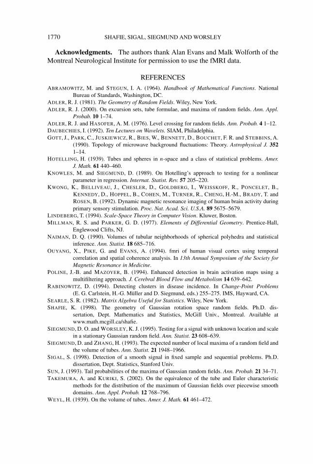
1770 SHAFIE, SIGAL, SIEGMUND AND WORSLEY
Acknowledgments. The authors thank Alan Evans and Malk Wolforth of theMontreal Neurological Institute for permission to use the fMRI data.
REFERENCES
ABRAMOWITZ, M. and STEGUN, I. A. (1964). Handbook of Mathematical Functions. NationalBureau of Standards, Washington, DC.
ADLER, R. J. (1981). The Geometry of Random Fields. Wiley, New York.ADLER, R. J. (2000). On excursion sets, tube formulae, and maxima of random fields. Ann. Appl.
Probab. 10 1–74.ADLER, R. J. and HASOFER, A. M. (1976). Level crossing for random fields. Ann. Probab. 4 1–12.DAUBECHIES, I. (1992). Ten Lectures on Wavelets. SIAM, Philadelphia.GOTT, J., PARK, C., JUSKIEWICZ, R., BIES, W., BENNETT, D., BOUCHET, F. R. and STEBBINS, A.
(1990). Topology of microwave background fluctuations: Theory. Astrophysical J. 3521–14.
HOTELLING, H. (1939). Tubes and spheres in n-space and a class of statistical problems. Amer.J. Math. 61 440–460.
KNOWLES, M. and SIEGMUND, D. (1989). On Hotelling’s approach to testing for a nonlinearparameter in regression. Internat. Statist. Rev. 57 205–220.
KWONG, K., BELLIVEAU, J., CHESLER, D., GOLDBERG, I., WEISSKOFF, R., PONCELET, B.,KENNEDY, D., HOPPEL, B., COHEN, M., TURNER, R., CHENG, H.-M., BRADY, T. andROSEN, B. (1992). Dynamic magnetic resonance imaging of human brain activity duringprimary sensory stimulation. Proc. Nat. Acad. Sci. U.S.A. 89 5675–5679.
LINDEBERG, T. (1994). Scale-Space Theory in Computer Vision. Kluwer, Boston.MILLMAN, R. S. and PARKER, G. D. (1977). Elements of Differential Geometry. Prentice-Hall,
Englewood Clifts, NJ.NAIMAN, D. Q. (1990). Volumes of tubular neighborhoods of spherical polyhedra and statistical
inference. Ann. Statist. 18 685–716.OUYANG, X., PIKE, G. and EVANS, A. (1994). fmri of human visual cortex using temporal
correlation and spatial coherence analysis. In 13th Annual Symposium of the Society forMagnetic Resonance in Medicine.
POLINE, J.-B. and MAZOYER, B. (1994). Enhanced detection in brain activation maps using amultifiltering approach. J. Cerebral Blood Flow and Metabolism 14 639–642.
RABINOWITZ, D. (1994). Detecting clusters in disease incidence. In Change-Point Problems(E. G. Carlstein, H.-G. Müller and D. Siegmund, eds.) 255–275. IMS, Hayward, CA.
SEARLE, S. R. (1982). Matrix Algebra Useful for Statistics. Wiley, New York.SHAFIE, K. (1998). The geometry of Gaussian rotation space random fields. Ph.D. dis-
sertation, Dept. Mathematics and Statistics, McGill Univ., Montreal. Available atwww.math.mcgill.ca/shafie.
SIEGMUND, D. O. and WORSLEY, K. J. (1995). Testing for a signal with unknown location and scalein a stationary Gaussian random field. Ann. Statist. 23 608–639.
SIEGMUND, D. and ZHANG, H. (1993). The expected number of local maxima of a random field andthe volume of tubes. Ann. Statist. 21 1948–1966.
SIGAL, S. (1998). Detection of a smooth signal in fixed sample and sequential problems. Ph.D.dissertation, Dept. Statistics, Stanford Univ.
SUN, J. (1993). Tail probabilities of the maxima of Gaussian random fields. Ann. Probab. 21 34–71.TAKEMURA, A. and KURIKI, S. (2002). On the equivalence of the tube and Euler characteristic
methods for the distribution of the maximum of Gaussian fields over piecewise smoothdomains. Ann. Appl. Probab. 12 768–796.
WEYL, H. (1939). On the volume of tubes. Amer. J. Math. 61 461–472.

RANDOM FIELDS AND fMRI DATA 1771
WILLMORE, T. J. (1959). An Introduction to Differential Geometry. Oxford Univ. Press.WORSLEY, K. J. (1994). Local maxima and the expected Euler characteristic of excursion sets of χ2,
F and t fields. Adv. in Appl. Probab. 26 13–42.WORSLEY, K. J. (2001). Testing for signals with unknown location and scale in a χ2 random field,
with an application to fMRI. Adv. in Appl. Probab. 33 773–793.WORSLEY, K., EVANS, A., MARRETT, S. and NEELIN, P. (1992). A three-dimensional statistical
analysis for cbf activation studies in human brain. J. Cerebral Blood Flow and Metabolism12 900–918.
K. SHAFIE
DEPARTMENT OF STATISTICS
FACULTY OF MATHEMATICAL SCIENCES
SHAHID BEHESHTI UNIVERSITY
EVEEN, TEHRAN
IRAN
E-MAIL: [email protected]
D. SIEGMUND
DEPARTMENT OF STATISTICS
STANFORD UNIVERSITY
STANFORD, CALIFORNIA
E-MAIL: [email protected]
B. SIGAL
DEPARTMENT OF RADIOLOGY
STANFORD UNIVERSITY
STANFORD, CALIFORNIA
E-MAIL: [email protected]
K. J. WORSLEY
DEPARTMENT OF MATHEMATICS
AND STATISTICS
MCGILL UNIVERSITY
MONTREAL, QUEBEC
CANADA H3A 2K6E-MAIL: [email protected]