Rotation matrix Representations of orientation Homogeneous ... · PDF fileRotation matrix...

INDUSTRIAL ROBOTICS Prof. Bruno SICILIANO

KINEMATICS

• relationship between joint positions and end-effector positionand orientation

Rotation matrix

Representations of orientation

Homogeneous transformations

Direct kinematics

Joint space and operational space

Kinematic calibration

Inverse kinematics problem


POSE OF A RIGID BODY

• Position

o′ =

o′xo′yo′z

• Orientation

x′ = x′xx + x′yy + x′zz

y′ = y′xx + y′yy + y′zz

z′ = z′xx + z′yy + z′zz


ROTATION MATRIX

R =

x′ y′ z′

=

x′Tx y′Tx z′Tx

x′Ty y′Ty z′Ty

x′Tz y′Tz z′Tz

RTR = I

RT = R−1


Elementary rotations

• rotation ofα aboutz

Rz(α) =

cosα −sinα 0sinα cosα 0

0 0 1


• rotation ofβ abouty

Ry(β) =

cosβ 0 sinβ0 1 0

−sinβ 0 cosβ

• rotation ofγ aboutx

Rx(γ) =

1 0 00 cos γ −sinγ0 sin γ cos γ


Representation of a vector

p =

pxpypz

p′ =

p′xp′yp′z

p =

x′ y′ z′

p′

= Rp′

p′ = RTp


• Example

px = p′x cosα− p′y sinα

py = p′x sinα+ p′y cosα

pz = p′z


Rotation of a vector

p = Rp′

pTp = p′TRTRp′

• Example

px = p′x cosα− p′y sinα

py = p′x sinα+ p′y cosα

pz = p′z

p = Rz(α)p′


• Rotation matrix

⋆ it describes the mutual orientation between two coordinateframes; its column vectors are the direction cosines of theaxes of the rotated frame with respect to the original frame

⋆ it represents the coordinate transformation between thecoordinates of a point expressed in two different frames(with common origin)

⋆ it is the operator that allows the rotation of a vector in thesame coordinate frame


COMPOSITION OF ROTATION MATRICES

p1 = R12p

2

p0 = R01p

1

p0 = R02p

2

Rji = (Ri

j)−1 = (Ri

j)T

• Current frame rotation

R02 = R0

1R12

• Fixed frame rotation

R02 = R1

2R01


• Example


EULER ANGLES

• rotation matrix

⋆ 9 parameters with 6 constraints

• minimal representation of orientation

⋆ 3 independent parameters


ZYZ angles

R(φ) = Rz(ϕ)Ry′(ϑ)Rz′′(ψ)

=

cϕcϑcψ − sϕsψ −cϕcϑsψ − sϕcψ cϕsϑsϕcϑcψ + cϕsψ −sϕcϑsψ + cϕcψ sϕsϑ

−sϑcψ sϑsψ cϑ


• Inverse problem

⋆ Given

R =

r11 r12 r13r21 r22 r23r31 r32 r33

the three ZYZ angles are (ϑ ∈ (0, π))

ϕ = Atan2(r23, r13)

ϑ = Atan2

(

√

r213 + r223, r33

)

ψ = Atan2(r32,−r31)

or (ϑ ∈ (−π, 0))

ϕ = Atan2(−r23,−r13)

ϑ = Atan2

(

−√

r213 + r223, r33

)

ψ = Atan2(−r32, r31)


RPY angles

R(φ) = Rz(ϕ)Ry(ϑ)Rx(ψ)

=

cϕcϑ cϕsϑsψ − sϕcψ cϕsϑcψ + sϕsψsϕcϑ sϕsϑsψ + cϕcψ sϕsϑcψ − cϕsψ−sϑ cϑsψ cϑcψ


• Inverse problem

⋆ Given

R =

r11 r12 r13r21 r22 r23r31 r32 r33

the three RPY angles are (ϑ ∈ (−π/2, π/2))

ϕ = Atan2(r21, r11)

ϑ = Atan2

(

−r31,√

r232 + r233

)

ψ = Atan2(r32, r33)

or (ϑ ∈ (π/2, 3π/2))

ϕ = Atan2(−r21,−r11)

ϑ = Atan2

(

−r31,−√

r232 + r233

)

ψ = Atan2(−r32,−r33)


ANGLE AND AXIS

R(ϑ, r) = Rz(α)Ry(β)Rz(ϑ)Ry(−β)Rz(−α)

sinα =ry

√

r2x + r2y

cosα =rx

√

r2x + r2y

sinβ =√

r2x + r2y cosβ = rz


R(ϑ, r) =

r2x(1 − cϑ) + cϑ rxry(1 − cϑ) − rzsϑ

rxry(1 − cϑ) + rzsϑ r2y(1 − cϑ) + cϑ

rxrz(1 − cϑ) − rysϑ ryrz(1 − cϑ) + rxsϑ

rxrz(1 − cϑ) + rysϑryrz(1 − cϑ) − rxsϑr2z(1 − cϑ) + cϑ

R(ϑ, r) = R(−ϑ,−r)


• Inverse problem

⋆ Given

R =

r11 r12 r13r21 r22 r23r31 r32 r33

the angle and axis of rotation are (sinϑ 6= 0)

ϑ = cos−1

(

r11 + r22 + r33 − 1

2

)

r =1

2 sinϑ

r32 − r23r13 − r31r21 − r12

withr2x + r2y + r2z = 1


UNIT QUATERNION

• 4-parameter representationQ = {η, ǫ}

η = cosϑ

2

ǫ = sinϑ

2r

η2 + ǫ2x + ǫ2y + ǫ2z = 1

⋆ (ϑ, r) and(−ϑ,−r) give the same quaternion

R(η, ǫ) =

2(η2 + ǫ2x) − 1 2(ǫxǫy − ηǫz) 2(ǫxǫz + ηǫy)

2(ǫxǫy + ηǫz) 2(η2 + ǫ2y) − 1 2(ǫyǫz − ηǫx)

2(ǫxǫz − ηǫy) 2(ǫyǫz + ηǫx) 2(η2 + ǫ2z) − 1


• Inverse problem

⋆ Given

R =

r11 r12 r13r21 r22 r23r31 r32 r33

the quaternion is (η ≥ 0)

η =1

2

√r11 + r22 + r33 + 1

ǫ =1

2

sgn (r32 − r23)√r11 − r22 − r33 + 1

sgn (r13 − r31)√r22 − r33 − r11 + 1

sgn (r21 − r12)√r33 − r11 − r22 + 1

• quaternion extracted fromR−1 = RT

Q−1 = {η,−ǫ}

• quaternion product

Q1 ∗ Q2 = {η1η2 − ǫT1 ǫ2, η1ǫ2 + η2ǫ1 + ǫ1 × ǫ2}


HOMOGENEOUS TRANSFORMATIONS

• Coordinate transformation (translation + rotation)

p0 = o01 + R0

1p1

• Inverse transformation

p1 = −R10o

01 + R1

0p0


• Homogeneous representation

p̃ =

p

1

• Homogeneous transformation matrix

A01 =

R01 o0

1

0T 1

• Coordinate transformation

p̃0 = A01p̃

1


• Inverse transformation

p̃1 = A10p̃

0 =(

A01

)−1p̃0

ove

A10 =

R10 −R1

0o01

0T 1

A−1 6= AT

• Sequence of coordinate transformations

p̃0 = A01A

12 . . .A

n−1n p̃n


DIRECT KINEMATICS

• Manipulator

⋆ series oflinks connected by means ofjoints

• Kinematic chain (from base to end-effector)

⋆ open (only one sequence)

⋆ closed (loop)

• Degree of freedom

⋆ associated with a joint articulation =joint variable


Base frame and end-effector frame

• Direct kinematics equation

T be (q) =

nbe(q) sbe(q) abe(q) pbe(q)

0 0 0 1


Two-link planar arm

T be (q) =

nbe sbe abe pbe

0 0 0 1

=

0 s12 c12 a1c1 + a2c120 −c12 s12 a1s1 + a2s121 0 0 00 0 0 1


Open chain

T 0n (q) = A0

1(q1)A12(q2) . . .A

n−1n (qn)

T be (q) = T b

0 T 0n (q)T n

e


Denavit–Hartenberg convention

• choose axiszi along axis of Jointi+ 1

• locateOi at the intersection of axiszi with the common normalto axeszi−1 andzi, andO′

i at intersection of common normalwith axiszi−1

• choose axisxi along common the normal to axeszi−1 andziwith positive direction from Jointi to Jointi+ 1

• choose axisyi so as to complete right-handed frame


• Nonunique definition of link frame:

⋆ for Frame0, only the direction of axisz0 is specified:thenO0 andx0 can be chosen arbitrarily

⋆ for Framen, since there is no Jointn+1, zn is not uniquelydefined whilexn has to be normal to axiszn−1); typicallyJointn is revolute and thuszn can be aligned withzn−1

⋆ when two consecutive axes are parallel, the common normalbetween them is not uniquely defined

⋆ when two consecutive axes intersect, the positive directionof xi is arbitrary

⋆ when Jointi is prismatic, only the direction ofzi−1 isspecified


Denavit–Hartenberg parameters

ai distance betweenOi andO′

i;

di coordinate ofO′

i alongzi−1;

αi angle between axeszi−1 andzi about axisxi to be taken positivewhen rotation is made counter-clockwise

ϑi angle between axesxi−1 andxi about axiszi−1 to be takenpositive when rotation is made counter-clockwise

• ai andαi are always constant

• if Joint i is revolute the variable isϑi

• if Joint i is prismatic the variable isdi


• Coordinate transformation

Ai−1

i′ =

cϑi−sϑi

0 0sϑi

cϑi0 0

0 0 1 di0 0 0 1

Ai′

i =

1 0 0 ai0 cαi

−sαi0

0 sαicαi

00 0 0 1

Ai−1

i (qi) = Ai−1

i′ Ai′

i =

cϑi−sϑi

cαisϑi

sαiaicϑi

sϑicϑicαi

−cϑisαi

aisϑi

0 sαicαi

di0 0 0 1


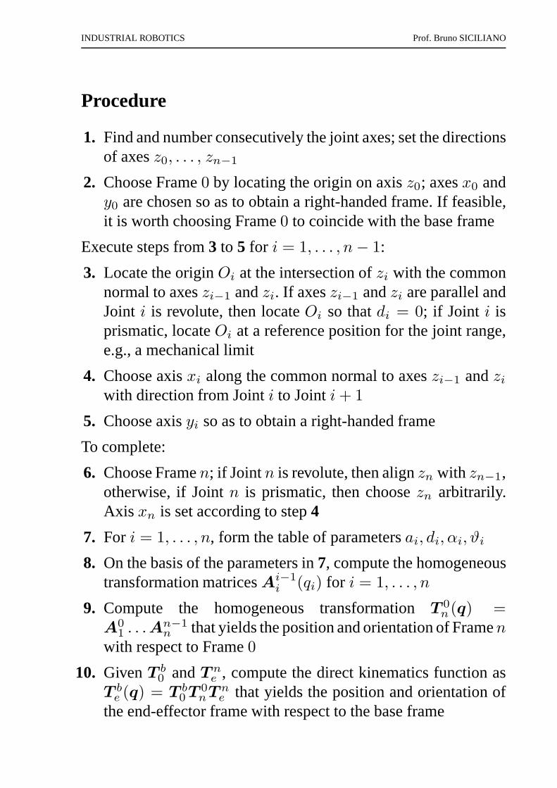
Procedure

1. Find and number consecutively the joint axes; set the directionsof axesz0, . . . , zn−1

2. Choose Frame0 by locating the origin on axisz0; axesx0 andy0 are chosen so as to obtain a right-handed frame. If feasible,it is worth choosing Frame0 to coincide with the base frame

Execute steps from3 to 5 for i = 1, . . . , n− 1:

3. Locate the originOi at the intersection ofzi with the commonnormal to axeszi−1 andzi. If axeszi−1 andzi are parallel andJoint i is revolute, then locateOi so thatdi = 0; if Joint i isprismatic, locateOi at a reference position for the joint range,e.g., a mechanical limit

4. Choose axisxi along the common normal to axeszi−1 andziwith direction from Jointi to Jointi+ 1

5. Choose axisyi so as to obtain a right-handed frame

To complete:

6. Choose Framen; if Jointn is revolute, then alignzn with zn−1,otherwise, if Jointn is prismatic, then choosezn arbitrarily.Axis xn is set according to step4

7. For i = 1, . . . , n, form the table of parametersai, di, αi, ϑi

8. On the basis of the parameters in7, compute the homogeneoustransformation matricesAi−1

i (qi) for i = 1, . . . , n

9. Compute the homogeneous transformationT 0n (q) =

A01 . . .A

n−1n that yields the position and orientation of Framen

with respect to Frame0

10. GivenT b0 andT n

e , compute the direct kinematics function asT be (q) = T b

0 T 0nT n

e that yields the position and orientation ofthe end-effector frame with respect to the base frame


Three–link planar arm


Link ai αi di ϑi

1 a1 0 0 ϑ1

2 a2 0 0 ϑ2

3 a3 0 0 ϑ3


Ai−1

i =

ci −si 0 aicisi ci 0 aisi0 0 1 00 0 0 1

i = 1, 2, 3

T 03 = A0

1A12A

23

=

c123 −s123 0 a1c1 + a2c12 + a3c123s123 c123 0 a1s1 + a2s12 + a3s1230 0 1 00 0 0 1


Spherical arm


Link ai αi di ϑi

1 0 −π/2 0 ϑ1

2 0 π/2 d2 ϑ2

3 0 0 d3 0


A01 =

c1 0 −s1 0s1 0 c1 00 −1 0 00 0 0 1

A1

2 =

c2 0 s2 0s2 0 −c2 00 1 0 d2

0 0 0 1

A23 =

1 0 0 00 1 0 00 0 1 d3

0 0 0 1

T 03 = A0

1A12A

23

=

c1c2 −s1 c1s2 c1s2d3 − s1d2

s1c2 c1 s1s2 s1s2d3 + c1d2

−s2 0 c2 c2d3

0 0 0 1


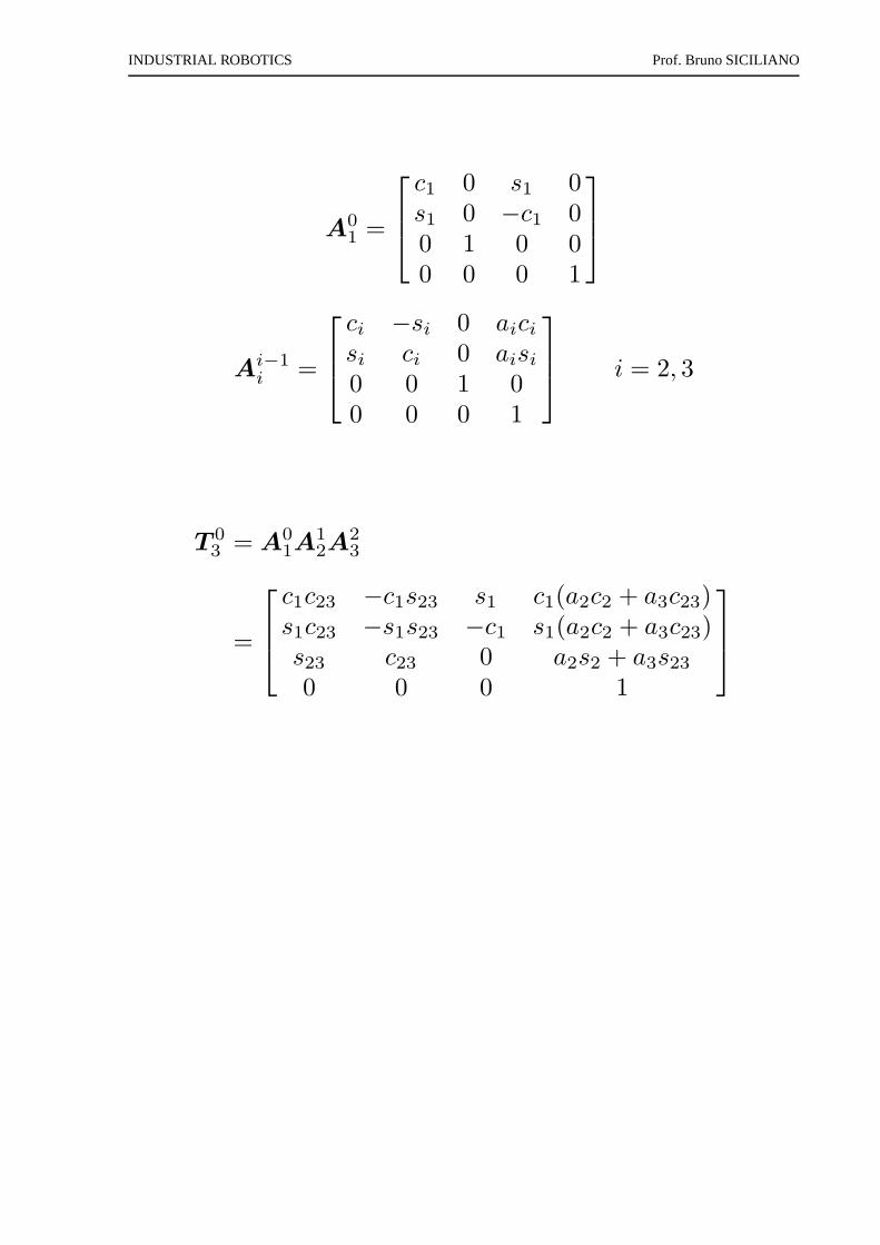
Anthropomorphic arm


Link ai αi di ϑi

1 0 π/2 0 ϑ1

2 a2 0 0 ϑ2

3 a3 0 0 ϑ3


A01 =

c1 0 s1 0s1 0 −c1 00 1 0 00 0 0 1

Ai−1

i =

ci −si 0 aicisi ci 0 aisi0 0 1 00 0 0 1

i = 2, 3

T 03 = A0

1A12A

23

=

c1c23 −c1s23 s1 c1(a2c2 + a3c23)s1c23 −s1s23 −c1 s1(a2c2 + a3c23)s23 c23 0 a2s2 + a3s230 0 0 1


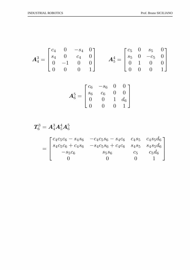
Spherical wrist


Link ai αi di ϑi

4 0 −π/2 0 ϑ4

5 0 π/2 0 ϑ5

6 0 0 d6 ϑ6


A34 =

c4 0 −s4 0s4 0 c4 00 −1 0 00 0 0 1

A4

5 =

c5 0 s5 0s5 0 −c5 00 1 0 00 0 0 1

A56 =

c6 −s6 0 0s6 c6 0 00 0 1 d6

0 0 0 1

T 36 = A3

4A45A

56

=

c4c5c6 − s4s6 −c4c5s6 − s4c6 c4s5 c4s5d6

s4c5c6 + c4s6 −s4c5s6 + c4c6 s4s5 s4s5d6

−s5c6 s5s6 c5 c5d6

0 0 0 1


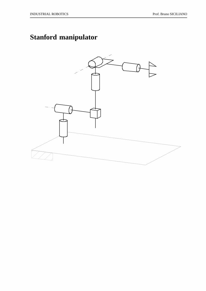
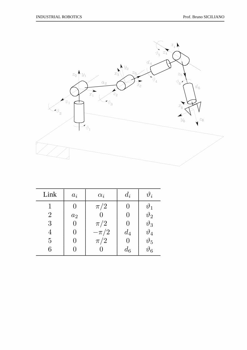
Stanford manipulator


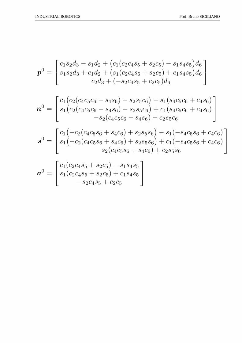
T 06 = T 0

3 T 36 =

n0 s0 a0 p0

0 0 0 1


p0 =

c1s2d3 − s1d2 +(

c1(c2c4s5 + s2c5) − s1s4s5)

d6

s1s2d3 + c1d2 +(

s1(c2c4s5 + s2c5) + c1s4s5)

d6

c2d3 + (−s2c4s5 + c2c5)d6

n0 =

c1(

c2(c4c5c6 − s4s6) − s2s5c6)

− s1(s4c5c6 + c4s6)

s1(

c2(c4c5c6 − s4s6) − s2s5c6)

+ c1(s4c5c6 + c4s6)−s2(c4c5c6 − s4s6) − c2s5c6

s0 =

c1(

−c2(c4c5s6 + s4c6) + s2s5s6)

− s1(−s4c5s6 + c4c6)

s1(

−c2(c4c5s6 + s4c6) + s2s5s6)

+ c1(−s4c5s6 + c4c6)s2(c4c5s6 + s4c6) + c2s5s6

a0 =

c1(c2c4s5 + s2c5) − s1s4s5s1(c2c4s5 + s2c5) + c1s4s5

−s2c4s5 + c2c5


Anthropomorphic arm with spherical wrist


Link ai αi di ϑi

1 0 π/2 0 ϑ1

2 a2 0 0 ϑ2

3 0 π/2 0 ϑ3

4 0 −π/2 d4 ϑ4

5 0 π/2 0 ϑ5

6 0 0 d6 ϑ6


A23 =

c3 0 s3 0s3 0 −c3 00 1 0 00 0 0 1

A3

4 =

c4 0 −s4 0s4 0 c4 00 −1 0 d4

0 0 0 1

p0 =

a2c1c2 + d4c1s23 + d6

(

c1(c23c4s5 + s23c5) + s1s4s5)

a2s1c2 + d4s1s23 + d6

(

s1(c23c4s5 + s23c5) − c1s4s5)

a2s2 − d4c23 + d6(s23c4s5 − c23c5)

n0 =

c1(

c23(c4c5c6 − s4s6) − s23s5c6)

+ s1(s4c5c6 + c4s6)

s1(

c23(c4c5c6 − s4s6) − s23s5c6)

− c1(s4c5c6 + c4s6)s23(c4c5c6 − s4s6) + c23s5c6

s0 =

c1(

−c23(c4c5s6 + s4c6) + s23s5s6)

+ s1(−s4c5s6 + c4c6)

s1(

−c23(c4c5s6 + s4c6) + s23s5s6)

− c1(−s4c5s6 + c4c6)−s23(c4c5s6 + s4c6) − c23s5s6

a0 =

c1(c23c4s5 + s23c5) + s1s4s5s1(c23c4s5 + s23c5) − c1s4s5

s23c4s5 − c23c5


DLR manipulator

Link ai αi di ϑi

1 0 π/2 0 ϑ1

2 0 π/2 0 ϑ2

3 0 π/2 d3 ϑ3

4 0 π/2 0 ϑ4

5 0 π/2 d5 ϑ5

6 0 π/2 0 ϑ6

7 0 0 d7 ϑ7


Ai−1

i =

ci 0 si 0

si 0 −ci 0

0 1 0 di

0 0 0 1

i = 1, . . . , 6

A67 =

c7 −s7 0 0

s7 c7 0 0

0 0 1 d7

0 0 0 1

p07 =

d3xd3 + d5xd5 + d7xd7d3yd3 + d5yd5 + d7yd7d3zd3 + d5zd5 + d7zd7

xd3 = c1s2

xd5 = c1(c2c3s4 − s2c4) + s1s3s4

xd7 = c1(c2k1 + s2k2) + s1k3

yd3 = s1s2

yd5 = s1(c2c3s4 − s2c4) − c1s3s4

yd7 = s1(c2k1 + s2k2) − c1k3

zd3 = −c2zd5 = c2c4 + s2c3s4

zd7 = s2(c3(c4c5s6 − s4c6) + s3s5s6) − c2k2

k1 = c3(c4c5s6 − s4c6) + s3s5s6

k2 = s4c5s6 + c4c6

k3 = s3(c4c5s6 − s4c6) − c3s5s6


n07 =

((xac5 + xcs5)c6 + xbs6)c7 + (xas5 − xcc5)s7((yac5 + ycs5)c6 + ybs6)c7 + (yas5 − ycc5)s7

(zac6 + zcs6)c7 + zbs7

s07 =

−((xac5 + xcs5)c6 + xbs6)s7 + (xas5 − xcc5)c7−((yac5 + ycs5)c6 + ybs6)s7 + (yas5 − ycc5)c7

−(zac6 + zcs6)s7 + zbc7

a07 =

(xac5 + xcs5)s6 − xbc6(yac5 + ycs5)s6 − ybc6

zas6 − zcc6

xa = (c1c2c3 + s1s3)c4 + c1s2s4

xb = (c1c2c3 + s1s3)s4 − c1s2c4

xc = c1c2s3 − s1c3

ya = (s1c2c3 − c1s3)c4 + s1s2s4

yb = (s1c2c3 − c1s3)s4 − s1s2c4

yc = s1c2s3 + c1c3

za = (s2c3c4 − c2s4)c5 + s2s3s5

zb = (s2c3s4 + c2c4)s5 − s2s3c5

zc = s2c3s4 + c2c4

⋆ seα7 = π/2

A67 =

c7 0 s7 a7c7

s7 0 −c7 a7s7

0 0 1 0

0 0 0 1


Humanoid manipulator

• Arms consisting of two DLR manipulators (α7 = π/2)

• Connecting device between the end-effector of the anthropomorphictorso and the base frames of the two manipulators

⋆ permits keeping the ‘chest’ of the humanoid manipulatoralways orthogonal to the ground (ϑ4 = −ϑ2 − ϑ3)

• Direct kinematics

T 0rh = T 0

3 T 3t T t

rTrrh

T 0lh = T 0

3 T 3t T t

l Tllh

T 3t =

c23 s23 0 0−s23 c23 0 0

0 0 1 00 0 0 1


⋆ T 03 like for anthropomorphic manipulator

⋆ T tr andT t

l depend onβ

⋆ T rrh andT l

lh like for DLR manipulator


JOINT SPACE AND OPERATIONAL SPACE

• Joint space

q =

q1...qn

⋆ qi = ϑi (revolute joint)

⋆ qi = di (prismatic joint)

• Operational space

x =

[

p

φ

]

⋆ p (position)

⋆ φ (orientation)

• Direct kinematics equation

x = k(q)


• Example

x =

pxpyφ

= k(q) =

a1c1 + a2c12 + a3c123a1s1 + a2s12 + a3s123

ϑ1 + ϑ2 + ϑ3


Workspace

• Reachable workspace

p = p(q) qim ≤ qi ≤ qiM i = 1, . . . , n

⋆ surface elements of planar, spherical, toroidal andcylindrical type

• Dexterous workspace

⋆ different orientations


• Example

⋆ admissible configurations


⋆ workspace


• Accuracy

⋆ deviation between the position reached in the assignedposture and the position computed via direct kinematics

⋆ typical values:(0.2, 1) mm

• Repeatability

⋆ measure of manipulator’s ability to return to a previouslyreached position

⋆ typical values:(0.02, 0.2) mm

• Kinematic redundancy

⋆ m < n (intrinsic)

⋆ r < m = n (functional)


KINEMATIC CALIBRATION

• Accurate estimates of DH parameters to improve manipulatoraccuracy

• Direct kinematics equation as a function of all parameters

x = k(a,α,d,ϑ)

xm measured pose

xn nominal pose (fixed parameters + joint variables)

∆x =∂k

∂a∆a +

∂k

∂α∆α +

∂k

∂d∆d +

∂k

∂ϑ∆ϑ

= Φ(ζn)∆ζ


⋆ l measurements (lm≫ 4n)

∆x̄ =

∆x1

...∆xl

=

Φ1

...Φl

∆ζ = Φ̄∆ζ

• Solution

∆ζ = (Φ̄T Φ̄)−1Φ̄T∆x̄

ζ′ = ζn +∆ζ

. . .until ∆ζ converges

⋆ more accurate estimates of fixed parameters

⋆ corrections on transducers measurements

Start-up

• (Home) reference posture


INVERSE KINEMATICS PROBLEM

• Direct kinematics

⋆ q =⇒ T

⋆ q =⇒ x

• Inverse kinematics

⋆ T =⇒ q

⋆ x =⇒ q

• Complexity

⋆ closed-form solution

⋆ multiple solutions

⋆ infinite solutions

⋆ no admissible solutions

• Intuition

⋆ algebraic

⋆ geometric

• Numerical techniques


Solution of three–link planar arm

• Algebraic solution

φ = ϑ1 + ϑ2 + ϑ3

pWx = px − a3cφ = a1c1 + a2c12

pWy = py − a3sφ = a1s1 + a2s12


c2 =p2Wx + p2

Wy − a21 − a2

2

2a1a2

s2 = ±√

1 − c22

ϑ2 = Atan2(s2, c2)

s1 =(a1 + a2c2)pWy − a2s2pWx

p2Wx + p2

Wy

c1 =(a1 + a2c2)pWx + a2s2pWy

p2Wy + p2

Wy

ϑ1 = Atan2(s1, c1)

ϑ3 = φ− ϑ1 − ϑ2


• Geometric solution

c2 =p2Wx + p2

Wy − a21 − a2

2

2a1a2

.

ϑ2 = cos−1(c2)

α = Atan2(pWy, pWx)

cβ

√

p2Wx + p2

Wy = a1 + a2c2

β = cos−1

p2Wx + p2

Wy + a21 − a2

2

2a1

√

p2Wx + p2

Wy

ϑ1 = α± β


Solution of manipulators with spherical wrist

pW = p − d6a

• Decoupled solution

⋆ compute wrist positionpW (q1, q2, q3)

⋆ solve inverse kinematics for(q1, q2, q3)

⋆ computeR03(q1, q2, q3)

⋆ computeR36(ϑ4, ϑ5, ϑ6) = R0

3TR

⋆ solve inverse kinematics for orientation(ϑ4, ϑ5, ϑ6)


Solution of spherical arm

(A01)

−1T 03 = A1

2A23

p1W =

pWxc1 + pWys1−pWz

−pWxs1 + pWyc1

=

d3s2−d3c2d2


c1 =1 − t2

1 + t2s1 =

2t

1 + t2

(d2 + pWy)t2 + 2pWxt+ d2 − pWy = 0

ϑ1 = 2Atan2(

−pWx ±√

p2Wx + p2

Wy − d22, d2 + pWy

)

pWxc1 + pWys1−pWz

=d3s2−d3c2

ϑ2 = Atan2(pWxc1 + pWys1, pWz)

d3 =√

(pWxc1 + pWys1)2 + p2Wz


Solution of anthropomorphic arm

pWx = c1(a2c2 + a3c23)

pWy = s1(a2c2 + a3c23)

pWz = a2s2 + a3s23

c3 =p2Wx + p2

Wy + p2Wz − a2

2 − a23

2a2a3

s3 = ±√

1 − c23

ϑ3 = Atan2(s3, c3)

⇓


ϑ3,I ∈ [−π, π]

ϑ3,II = −ϑ3,I


c2 =±

√

p2Wx + p2

Wy(a2 + a3c3) + pWza3s3

a22 + a2

3 + 2a2a3c3

s2 =pWz(a2 + a3c3) ∓

√

p2Wx + p2

Wya3s3

a22 + a2

3 + 2a2a3c3

ϑ2 = Atan2(s2, c2)

⇓

⋆ for s+3 =√

1 − c23:

ϑ2,I = Atan2(

(a2 + a3c3)pWz − a3s+

3

√

p2Wx + p2

Wy,

(a2 + a3c3)√

p2Wx + p2

Wy + a3s+

3 pWz

)

ϑ2,II = Atan2(

(a2 + a3c3)pWz + a3s+

3

√

p2Wx + p2

Wy,

−(a2 + a3c3)√

p2Wx + p2

Wy + a3s+3 pWz

)

⋆ for s−3 = −√

1 − c23:

ϑ2,III = Atan2(

(a2 + a3c3)pWz − a3s−

3

√

p2Wx + p2

Wy,

(a2 + a3c3)√

p2Wx + p2

Wy + a3s−

3 pWz

)

ϑ2,IV = Atan2(

(a2 + a3c3)pWz + a3s−

3

√

p2Wx + p2

Wy,

−(a2 + a3c3)√

p2Wx + p2

Wy + a3s−

3 pWz

)


ϑ1,I = Atan2(pWy, pWx)

ϑ1,II = Atan2(−pWy,−pWx)

• Four admissible configurations

(ϑ1,I , ϑ2,I , ϑ3,I) (ϑ1,I , ϑ2,III , ϑ3,II)

(ϑ1,II , ϑ2,II , ϑ3,I) (ϑ1,II , ϑ2,IV , ϑ3,II)

⋆ infinite solutions (kinematic singularity)

pWx = 0 pWy = 0


Solution of spherical wrist

R36 =

n3x s3x a3

x

n3y s3y a3

y

n3z s3z a3

z

ϑ4 = Atan2(a3y, a

3x)

ϑ5 = Atan2(√

(a3x)

2 + (a3y)

2, a3z

)

ϑ6 = Atan2(s3z,−n3z)

ϑ4 = Atan2(−a3y,−a3

x)

ϑ5 = Atan2(

−√

(a3x)

2 + (a3y)

2, a3z

)

ϑ6 = Atan2(−s3z, n3z)

Rotation matrix Representations of orientation Homogeneous ... · PDF fileRotation matrix...

Documents

Transcript of Rotation matrix Representations of orientation Homogeneous ... · PDF fileRotation matrix...