SABRE Training

Candidate:

Nazir A Ganai

SK University of Agricultural Sciences and Technology Kashmir India

Host Institute:Department of Genetics and Genomics

Roslin Biocenter, Edinburgh University Scotland

Advisor:

Dr DJ de KoningPeriod:

17-11-2008 to 31-12-2008

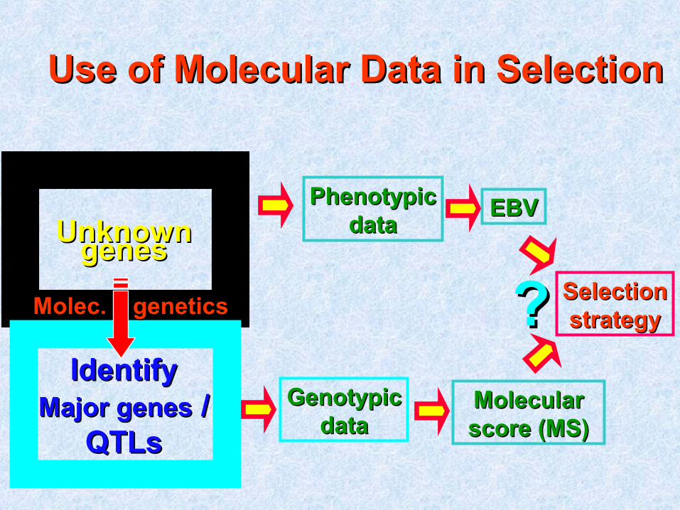
Use of Molecular Data in SelectionUse of Molecular Data in Selection

UnknownUnknowngenesgenes

IdentifyIdentifyMajor genesMajor genes / /

QTLsQTLs

PhenotypicPhenotypicdatadata

EBVEBV

GenotypicGenotypicdatadata

SelectionSelectionstrategystrategyMolec. geneticsMolec. genetics ??

Molecular Molecular score (MS)score (MS)

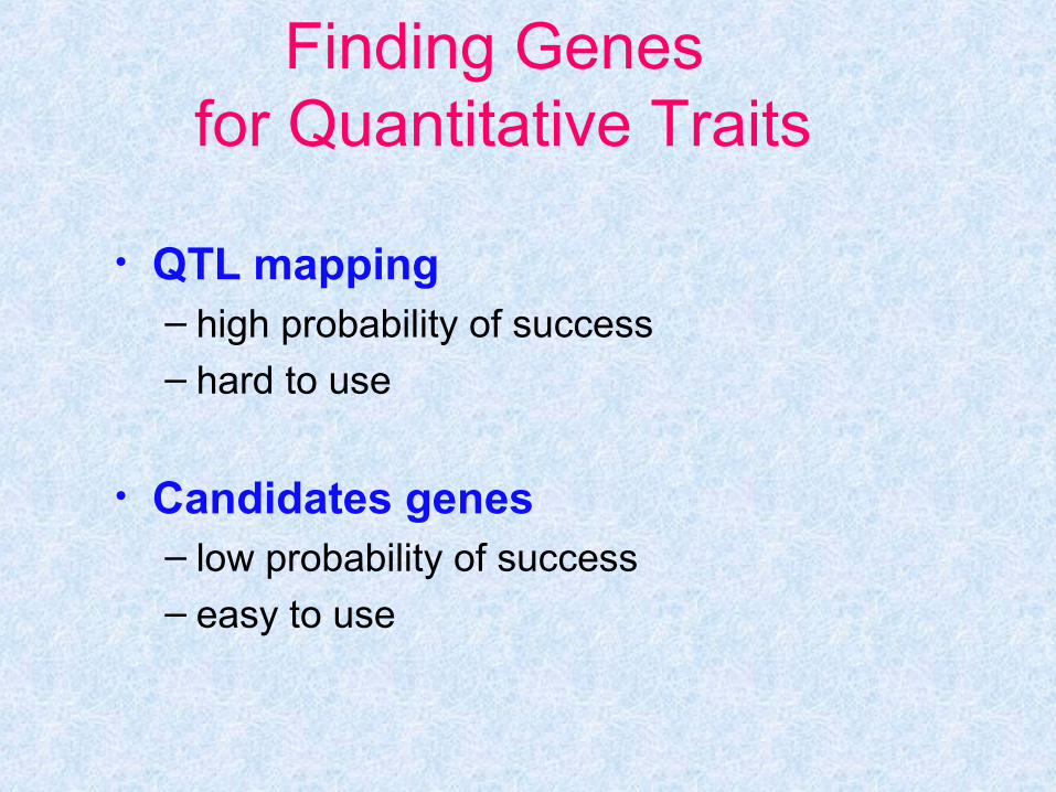
Finding Genes for Quantitative Traits

• QTL mapping– high probability of success– hard to use

• Candidates genes– low probability of success– easy to use

QTL mapping• QTL : a region of the genome that is associated with an effect on a quantitative trait.

– a QTL can be a single gene, or it may be a cluster of linked genes

– the aim of QTL mapping is primarily to:• detect which regions (QTL) of the genome affect the trait, • describe the effect of the QTL on the trait

– how much of the variation for the trait is caused by a QTL – what is the gene action associated with the QTL - additive /domininat

effect? – which marker allele is associated with the favorable effect?

– Use of QTLs in MAS:• Assign breeding values to lines or families based on their genotypes at

one or more QTLs. In this way we can use information obtained in QTL mapping experiments for applied marker-assisted breeding strategies.

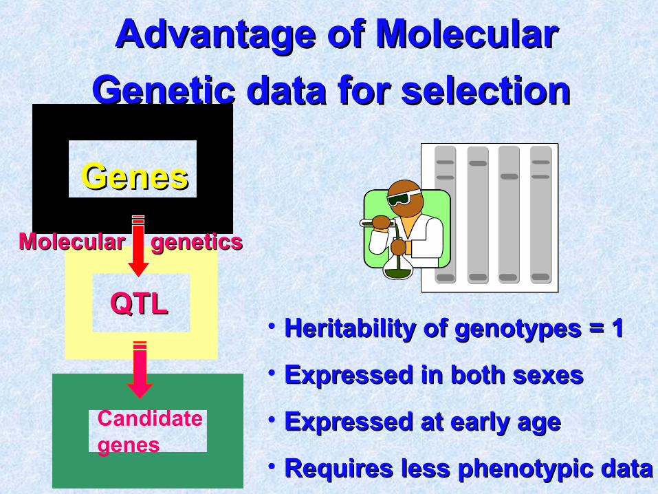
GenesGenes

Advantage of Molecular Advantage of Molecular

Genetic data for selection Genetic data for selection

Molecular geneticsMolecular genetics

QTLQTL• Heritability of genotypes = 1Heritability of genotypes = 1

• Expressed in both sexesExpressed in both sexes

• Expressed at early ageExpressed at early age

• Requires less phenotypic dataRequires less phenotypic data

Candidate genes

QTL Analysis

• Detection of QTLs depends on five main factors:– How tightly linked the QTL is to a marker

• Linkage Mapping – exploits LD within families• LD Mapping – exploits LD across the families in a population

– The size of effect • Small QTL effect – Low power of detection• Large QTL effect – high power of detection

– Experimental design: • Inbred / Line bred cross progeny

– Backcross– F2– Recombinant Inbred Lines

• Segregating populations– Full sib families– Half sib families– Three generation families (Grand Daughter Design)– Selective genotyping– Selective DNA pooling (Bulk segregant analysis)

– The size of the population scored – The heritability of the involved trait

Techniques of QTL mapping

• Single marker analysis – each marker - trait association test is performed independently. – Only detects linkage between marker and a QTL – Does not estimate position and effect of QTL.

• Flanking / interval marker mapping – – a separate analysis is performed for each pair of adjacent marker loci. – produces a slight increase in the power of detection, compared to single

marker, – much greater precision in estimating QTL effects and position.

• Composite multipoint mapping – – considers all the linked markers on a chromosome simultaneously.– reduce the bias that is present using interval mapping approaches when

two or more QTL are linked to the markers.

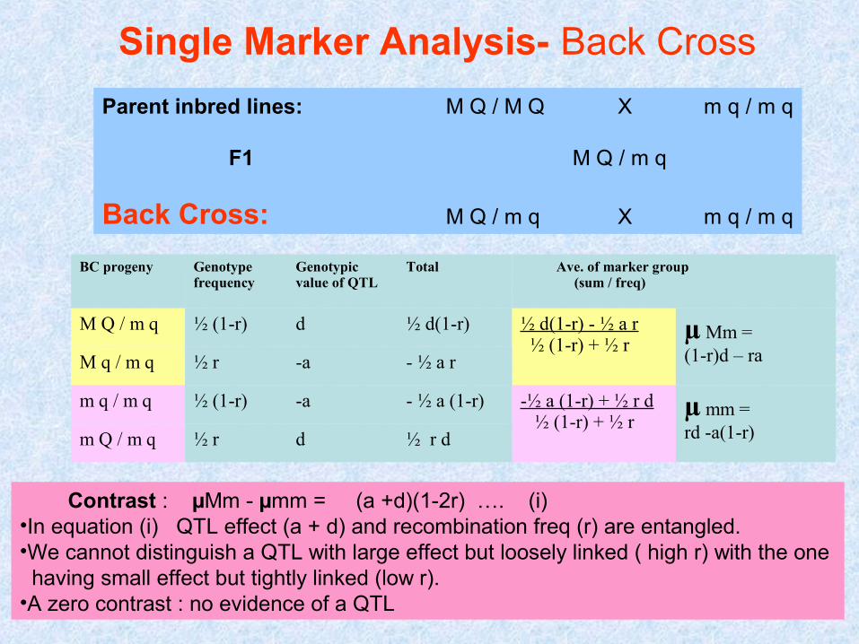
BC progeny Genotype frequency

Genotypic value of QTL

Total Ave. of marker group (sum / freq)

M Q / m q ½ (1-r) d ½ d(1-r) ½ d(1-r) - ½ a r ½ (1-r) + ½ r

µ Mm = (1-r)d – raM q / m q ½ r -a - ½ a r

m q / m q ½ (1-r) -a - ½ a (1-r) -½ a (1-r) + ½ r d ½ (1-r) + ½ r

µ mm = rd -a(1-r)m Q / m q ½ r d ½ r d

Single Marker Analysis- Back Cross

Parent inbred lines: M Q / M Q X m q / m q

F1 M Q / m q

Back Cross: M Q / m q X m q / m q

Contrast : µMm - µmm = (a +d)(1-2r) …. (i)•In equation (i) QTL effect (a + d) and recombination freq (r) are entangled. •We cannot distinguish a QTL with large effect but loosely linked ( high r) with the one having small effect but tightly linked (low r).•A zero contrast : no evidence of a QTL

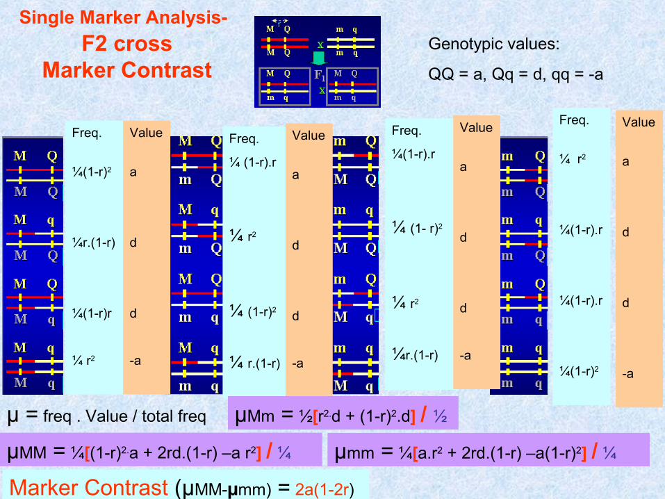
Genotypic values:

QQ = a, Qq = d, qq = -a

Freq.

¼(1-r)2

¼r.(1-r)

¼(1-r)r

¼ r2

Freq.

¼ (1-r).r

¼ r2

¼ (1-r)2

¼ r.(1-r)

Freq.

¼(1-r).r

¼ (1- r)2

¼ r2

¼r.(1-r)

Freq.

¼ r2

¼(1-r).r

¼(1-r).r

¼(1-r)2

Value

a

d

d

-a

Value

a

d

d

-a

Value

a

d

d

-a

Value

a

d

d

-a

µ = freq . Value / total freq µMM = ¼[(1-r)2.a + 2rd.(1-r) –a r2] / ¼

µMm = ½[r2.d + (1-r)2.d] / ½

µmm = ¼[a.r2 + 2rd.(1-r) –a(1-r)2] / ¼

Marker Contrast (µMM-µmm) = 2a(1-2r)

Single Marker Analysis- F2 cross

Marker Contrast

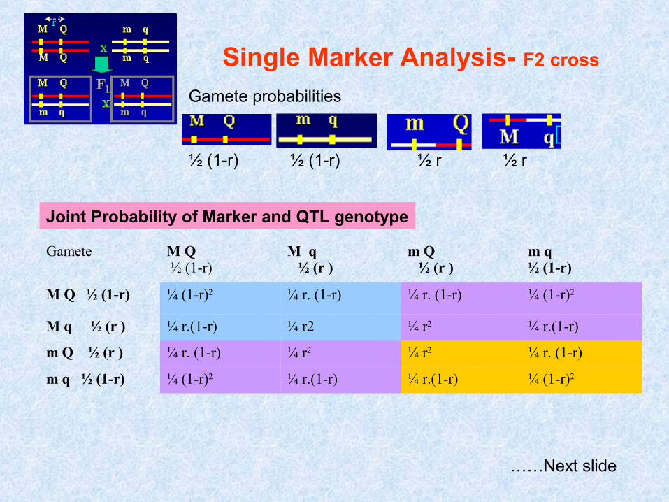
Single Marker Analysis- F2 cross

Gamete probabilities

½ (1-r) ½ (1-r) ½ r ½ r

Gamete M Q ½ (1-r)

M q ½ (r )

m Q ½ (r )

m q½ (1-r)

M Q ½ (1-r) ¼ (1-r)2 ¼ r. (1-r) ¼ r. (1-r) ¼ (1-r)2

M q ½ (r ) ¼ r.(1-r) ¼ r2 ¼ r2 ¼ r.(1-r)

m Q ½ (r ) ¼ r. (1-r) ¼ r2 ¼ r2 ¼ r. (1-r)

m q ½ (1-r) ¼ (1-r)2 ¼ r.(1-r) ¼ r.(1-r) ¼ (1-r)2

Joint Probability of Marker and QTL genotype

……Next slide

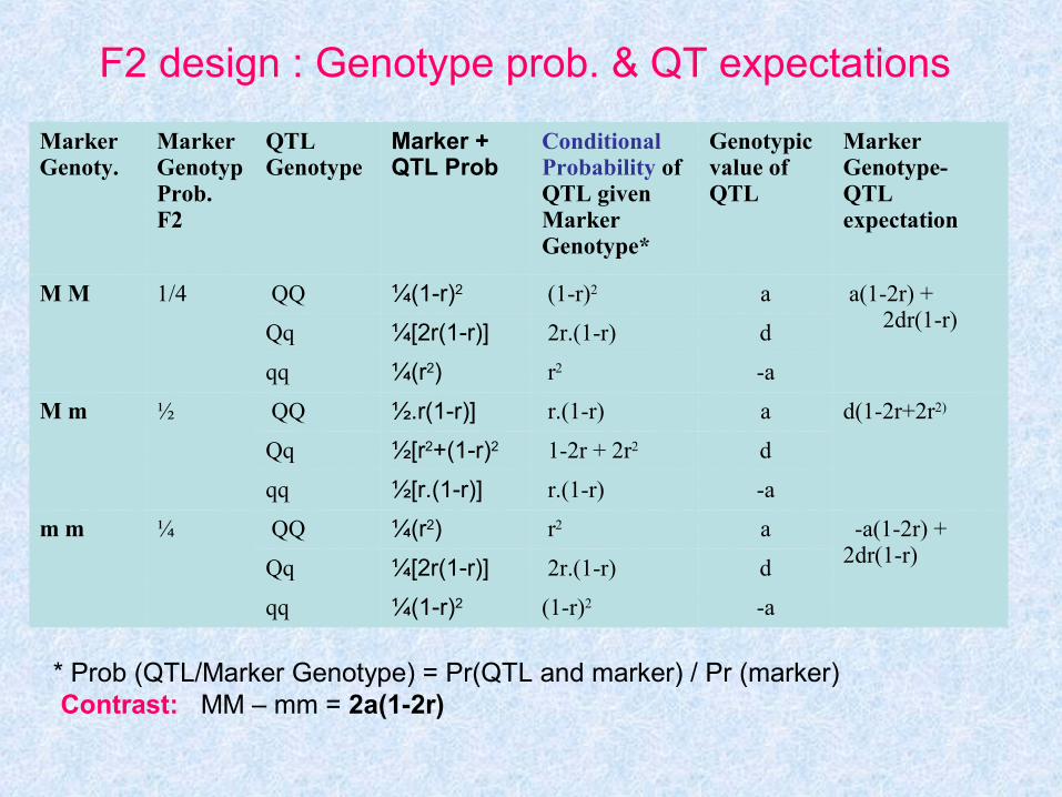
F2 design : Genotype prob. & QT expectations

MarkerGenoty.

MarkerGenotypProb. F2

QTLGenotype

Marker +QTL Prob

ConditionalProbability ofQTL givenMarkerGenotype*

Genotypicvalue ofQTL

MarkerGenotype-QTLexpectation

M M 1/4 QQ ¼(1-r)2 (1-r)2 a a(1-2r) + 2dr(1-r)Qq ¼[2r(1-r)] 2r.(1-r) d

qq ¼(r2) r2 -a

M m ½ QQ ½.r(1-r)] r.(1-r) a d(1-2r+2r2)

Qq ½[r2+(1-r)2 1-2r + 2r2 d

qq ½[r.(1-r)] r.(1-r) -a

m m ¼ QQ ¼(r2) r2 a -a(1-2r) + 2dr(1-r)Qq ¼[2r(1-r)] 2r.(1-r) d

qq ¼(1-r)2 (1-r)2 -a

* Prob (QTL/Marker Genotype) = Pr(QTL and marker) / Pr (marker) Contrast: MM – mm = 2a(1-2r)

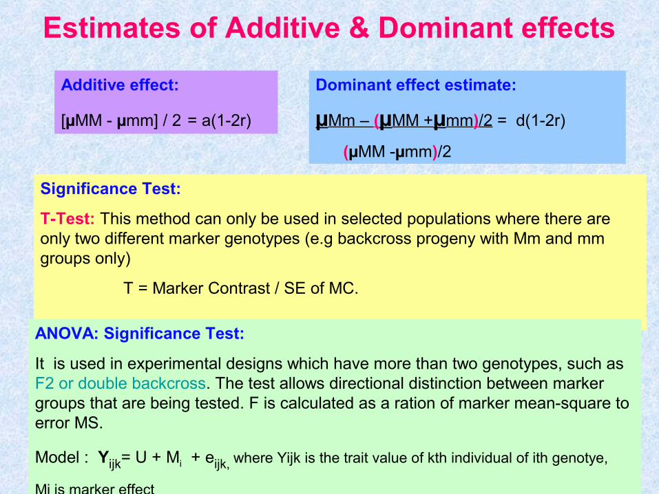
Estimates of Additive & Dominant effects

Additive effect:

[µMM - µmm] / 2 = a(1-2r)

Dominant effect estimate:

µMm – (µMM +µmm)/2 = d(1-2r)

(µMM -µmm)/2

Significance Test:

T-Test: This method can only be used in selected populations where there are only two different marker genotypes (e.g backcross progeny with Mm and mm groups only)

T = Marker Contrast / SE of MC.

ANOVA: Significance Test:

It is used in experimental designs which have more than two genotypes, such as F2 or double backcross. The test allows directional distinction between marker groups that are being tested. F is calculated as a ration of marker mean-square to error MS.

Model : Yijk= U + Mi + eijk, where Yijk is the trait value of kth individual of ith genotye,

Mi is marker effect

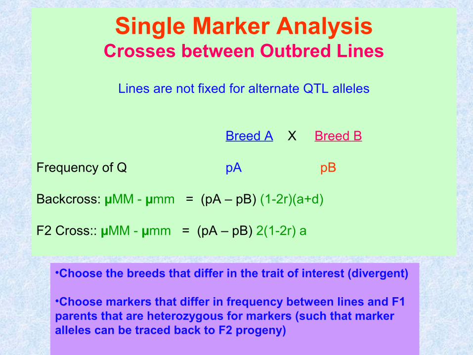
Single Marker AnalysisCrosses between Outbred Lines

Lines are not fixed for alternate QTL alleles

Breed A X Breed B

Frequency of Q pA pB

Backcross: µMM - µmm = (pA – pB) (1-2r)(a+d)

F2 Cross:: µMM - µmm = (pA – pB) 2(1-2r) a

•Choose the breeds that differ in the trait of interest (divergent)

•Choose markers that differ in frequency between lines and F1 parents that are heterozygous for markers (such that marker alleles can be traced back to F2 progeny)

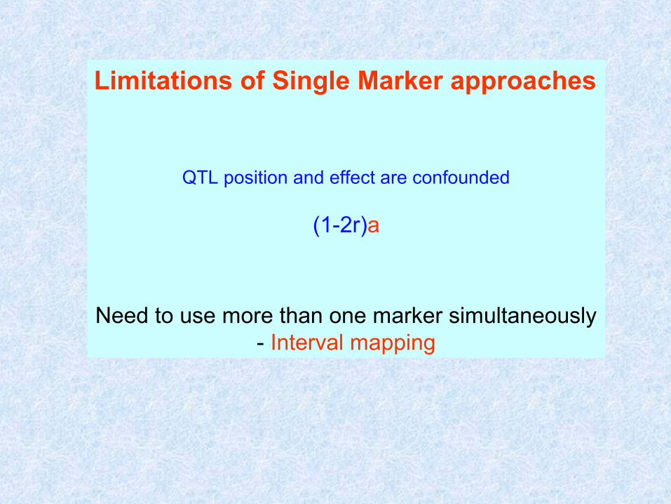
Limitations of Single Marker approaches

QTL position and effect are confounded

(1-2r)a

Need to use more than one marker simultaneously- Interval mapping

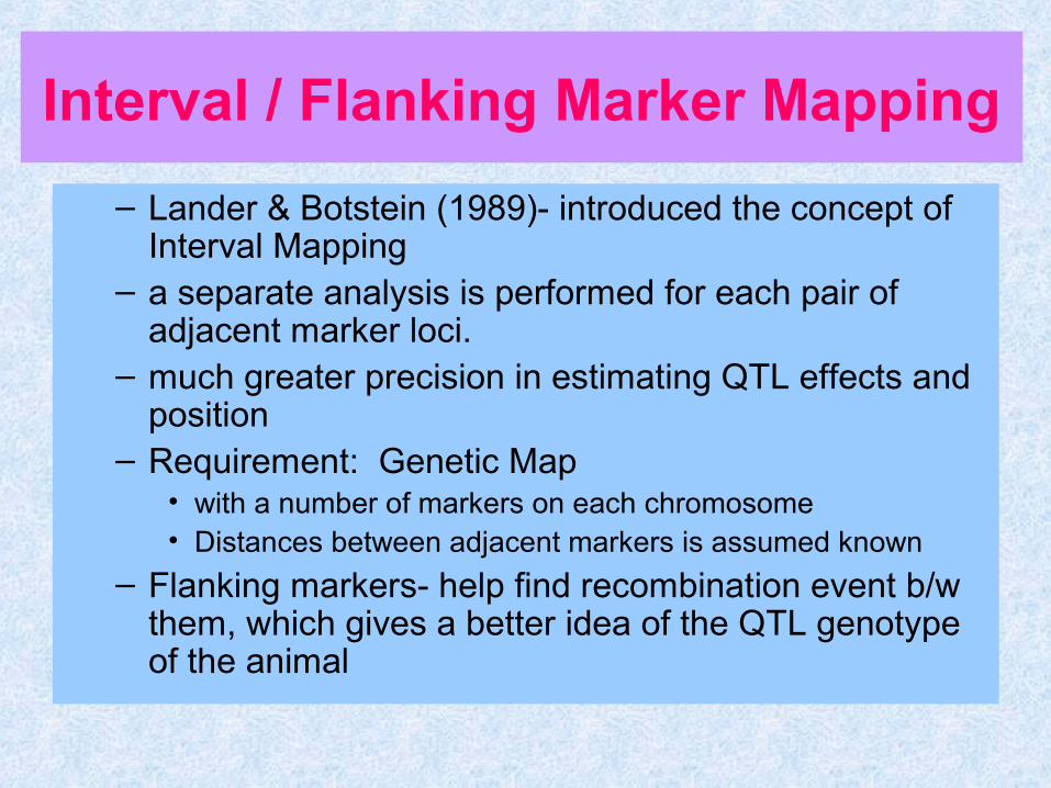
Interval / Flanking Marker Mapping

– Lander & Botstein (1989)- introduced the concept of Interval Mapping

– a separate analysis is performed for each pair of adjacent marker loci.

– much greater precision in estimating QTL effects and position

– Requirement: Genetic Map • with a number of markers on each chromosome• Distances between adjacent markers is assumed known

– Flanking markers- help find recombination event b/w them, which gives a better idea of the QTL genotype of the animal

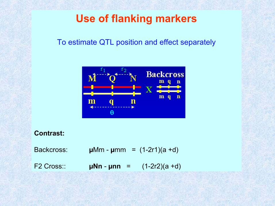
Use of flanking markers

To estimate QTL position and effect separately

Contrast:

Backcross: µMm - µmm = (1-2r1)(a +d)

F2 Cross:: µNn - µnn = (1-2r2)(a +d)

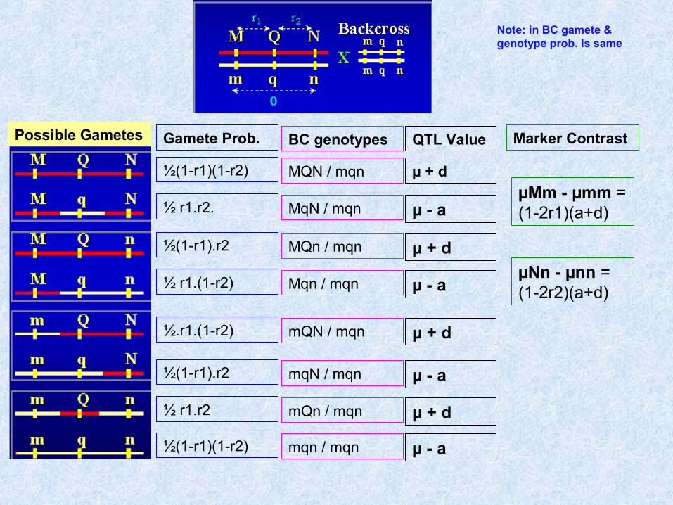
Possible Gametes Gamete Prob.

½(1-r1)(1-r2)

½ r1.r2.

½(1-r1).r2

½ r1.(1-r2)

½.r1.(1-r2)

½(1-r1).r2

½ r1.r2

½(1-r1)(1-r2)

BC genotypes

MQN / mqn

MqN / mqn

MQn / mqn

Mqn / mqn

mQN / mqn

mqN / mqn

mQn / mqn

mqn / mqn

QTL Value

µ + d

µ - a

µ + d

µ - a

µ + d

µ - a

µ + d

µ - a

Marker Contrast

µMm - µmm = (1-2r1)(a+d)

µNn - µnn = (1-2r2)(a+d)

Note: in BC gamete & genotype prob. Is same

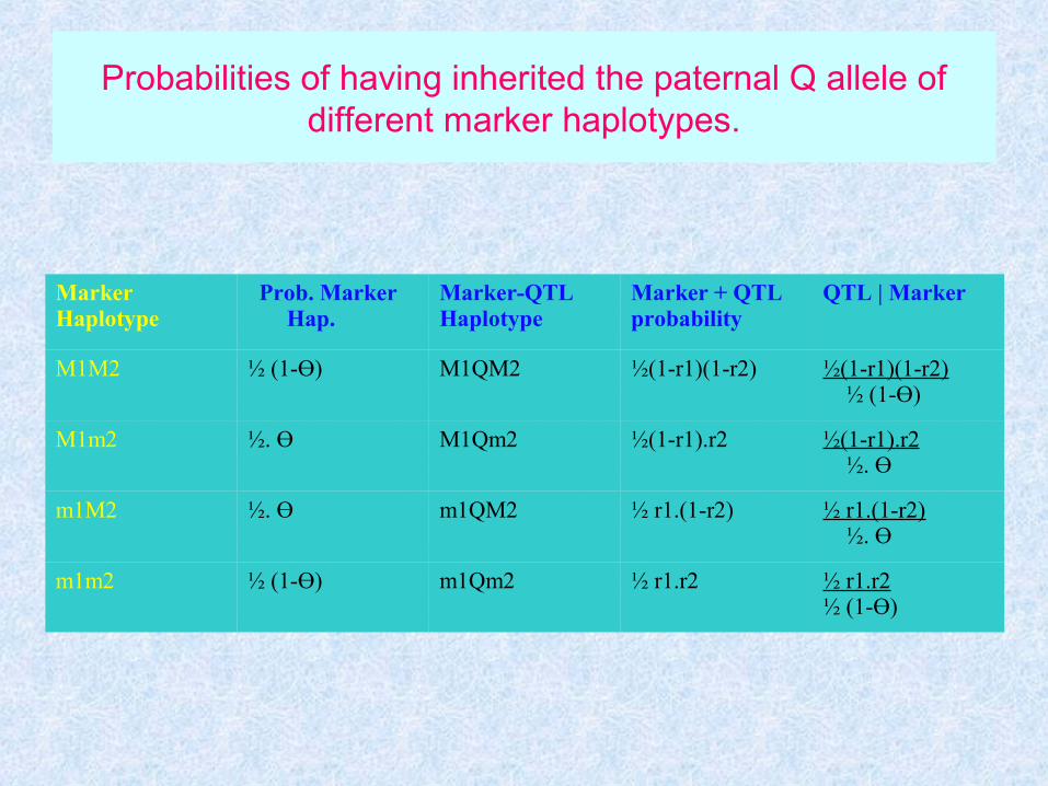
Probabilities of having inherited the paternal Q allele of different marker haplotypes.

MarkerHaplotype

Prob. Marker Hap.

Marker-QTLHaplotype

Marker + QTLprobability

QTL | Marker

M1M2 ½ (1-Ө) M1QM2 ½(1-r1)(1-r2) ½(1-r1)(1-r2) ½ (1-Ө)

M1m2 ½. Ө M1Qm2 ½(1-r1).r2 ½(1-r1).r2 ½. Ө

m1M2 ½. Ө m1QM2 ½ r1.(1-r2) ½ r1.(1-r2) ½. Ө

m1m2 ½ (1-Ө) m1Qm2 ½ r1.r2 ½ r1.r2½ (1-Ө)

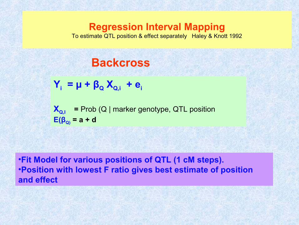
Regression Interval MappingTo estimate QTL position & effect separately Haley & Knott 1992

Yi = µ + βQ XQ,i + ei

XQ,I = Prob (Q | marker genotype, QTL position

E(βQ) = a + d

•Fit Model for various positions of QTL (1 cM steps).•Position with lowest F ratio gives best estimate of position and effect

Backcross

Interval / Flanking Marker Mapping F2 Cross between Inbred Lines

Parents: MQN / MQN X mqn / mqnF1 : MQN / mqn

Markers Pr (QQ|markers) Pr (Qq| markers) Pr (qq|markers) Additive Coef (X a)Pr (QQ) – Pr (qq)

Domin. Coef (X d) Pr (Qq)

MM NN f (r1,r2, Ө) f (r1,r2, Ө) f (r1,r2, Ө) f (r1,r2, Ө) f (r1,r2, Ө)MM Nn

MM nnMm NNMm NnMm nnmm NNmm Nnmm nn

Yi = µ + βa Xadd,i + βd Xdom,i + ei

E(βa) = a E(βd) = d

Genome Scan:

Fit Regression Model at every position along the chromosome

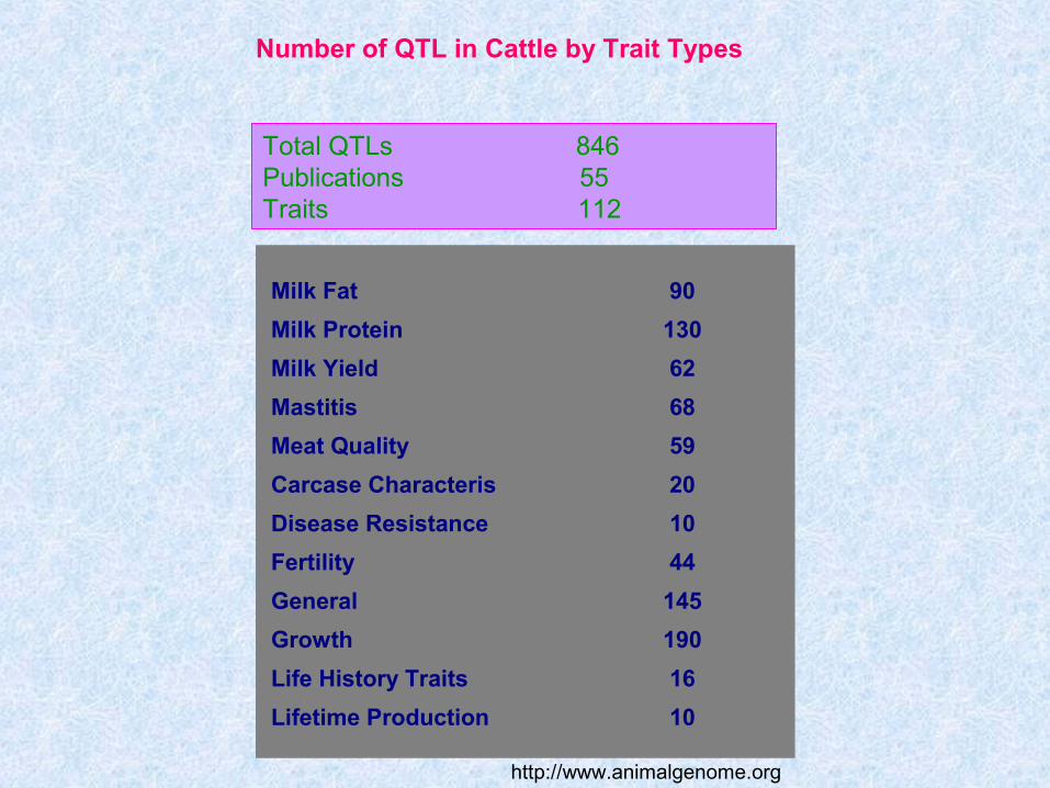
Number of QTL in Cattle by Trait Types

Milk Fat 90

Milk Protein 130

Milk Yield 62

Mastitis 68

Meat Quality 59

Carcase Characteris 20

Disease Resistance 10

Fertility 44

General 145

Growth 190

Life History Traits 16

Lifetime Production 10

http://www.animalgenome.org

Total QTLs 846Publications 55Traits 112

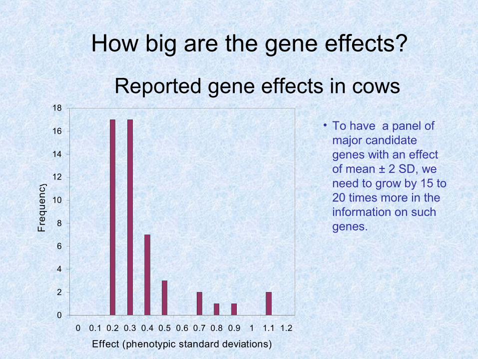
How big are the gene effects?

0

2

4

6

8

10

12

14

16

18

0 0.1 0.2 0.3 0.4 0.5 0.6 0.7 0.8 0.9 1 1.1 1.2

Effect (phenotypic standard deviations)

Fre

qu

en

cy

Reported gene effects in cows

• To have a panel of major candidate genes with an effect of mean ± 2 SD, we need to grow by 15 to 20 times more in the information on such genes.

QTL in SelectionQTL in Selection

• Use of QTL detected in breed crossesUse of QTL detected in breed crosses

• Marker-assisted introgressionMarker-assisted introgression

• Marker-assisted selection in crossesMarker-assisted selection in crosses

• Marker-assisted selection within breedsMarker-assisted selection within breeds

• Gene Assisted Selection (candidate genes)Gene Assisted Selection (candidate genes)

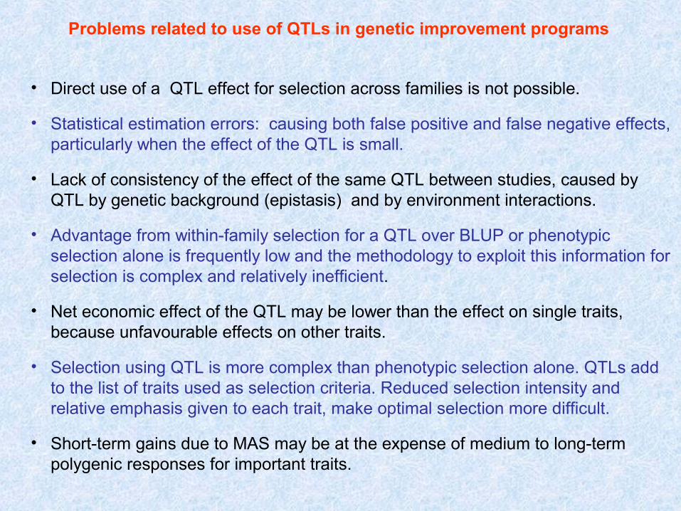
• Direct use of a QTL effect for selection across families is not possible.

• Statistical estimation errors: causing both false positive and false negative effects, particularly when the effect of the QTL is small.

• Lack of consistency of the effect of the same QTL between studies, caused by QTL by genetic background (epistasis) and by environment interactions.

• Advantage from within-family selection for a QTL over BLUP or phenotypic selection alone is frequently low and the methodology to exploit this information for selection is complex and relatively inefficient.

• Net economic effect of the QTL may be lower than the effect on single traits, because unfavourable effects on other traits.

• Selection using QTL is more complex than phenotypic selection alone. QTLs add to the list of traits used as selection criteria. Reduced selection intensity and relative emphasis given to each trait, make optimal selection more difficult.

• Short-term gains due to MAS may be at the expense of medium to long-term polygenic responses for important traits.

Problems related to use of QTLs in genetic improvement programs