roshan qt

8/11/2019 roshan qt

http://slidepdf.com/reader/full/roshan-qt 1/28

8/11/2019 roshan qt


ACKNOWLEDGEMENT

The project assigned to me for a good learning package consisting of practicality

and etiquettes of corporate world along with fun and excitement. It provided me

an opportunity to implement theoretical knowledge into practical and to learn

more from it.

It is my great pleasure to express my gratitude to my internal guide Mr. Krishna

Murti sir who encouraged, motivated and guided me through out my live project.

8/11/2019 roshan qt


METHODOLOGY

Method

Application

Data

Data Analysis

Conclusion

TOPICS COVERED

Graph and charts

Descriptive statistics

Probability

Probability Distribution

covariance

Estimation

Hypothesis

8/11/2019 roshan qt


METHOD

GRAPH AND CHARTS

HISTOGRAM

A Histogram is a graphical display of data using bars of different heights

A Frequency Histogram is a special histogram that uses vertical columns to show

frequencies (how many times each score occurs)

A histogram displays continuous data in ordered columns. Categories are of

continuous measure such as time, inches, temperature, etc.

Advantages:

1. Visually strong

2. Can compare to normal curve

3. Usually vertical axis is a frequency count of items falling into each category

Disadvantages:

1. Cannot read exact values because data is grouped into categories

2. More difficult to compare two data sets

3. Use only with continuous data

8/11/2019 roshan qt


8/11/2019 roshan qt


Disadvantages:

1. Graph categories can be reordered to emphasize certain effects

2. Use only with discrete data

PIE CHART

A Pie Chart is a circular Chart divided into sectors, each sector shows the relative

size of each value.

Advantages:

1. Visually appealing

2. Shows percent of total for each category

Disadvantages:

1. No exact numerical data

2. Hard to compare 2 data sets

3. "Other" category can be a problem

4. Total unknown unless specified

5. Best for 3 to 7 categories

6. Use only with discrete data

8/11/2019 roshan qt


Burger & More Food Joint

HISTOGRAM

Year Sales

2010 5000

2011 10000

2012 7000

2013 15000

The histogram tells us about the relationship between the sales and number of

years. It is an easy way to check the performance of the restaurant.

0

2000

4000

6000

8000

10000

12000

14000

16000

2010 2011 2012 2013

SALES

8/11/2019 roshan qt


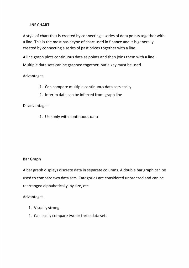
LINE CHART

YEAR Table Service Take Away Home Delivery

2010 3000 2000 1000

2011 6000 2000 2000

2012 4000 2000 1000

2013 8000 4000 3000

0

1000

2000

3000

4000

5000

6000

7000

8000

9000

2010 2011 2012 2013

Table Service

Take Away

Home Delivery

8/11/2019 roshan qt


PIE CHART

ITEMS CONSUMPTION IN %

BURGERS 33

SANDWICH 20PASTAS 16

SUBS 14

RAPS 17

PIE Chart gives combination was various consumption pattern of customers in

the restaurant also it helps the owner to know the demand is more for which

type of food.

CONSUMPTION IN %

BURGERS

SANDWITCHS

PASTAS

SUBS

RAPS

8/11/2019 roshan qt


DATA

Mean, Median and mode

MONTH SALESJanuary 20000

February 5000

March 3000

April 30000

May 25000

June 3000

July 7000

August 15000

September 30000

October 40000

November 50000

December 60000

TOTAL 288000

Standard Deviation and Variance

FOOD ITEMS PRICE(X) X-x (x-x)2sq

Burger 120 -30 900

Sandwich 140 -10 100

Pasta 150 0 0

Subs 160 10 100

Raps 180 30 900

TOTAL 750 TOTAL 2000

8/11/2019 roshan qt


Probability

TYPE OF CUSTOMERS FREQUENCY RELATIVE FREQUENCY

Students(S) 20 0.2

Couples(C) 30 0.3Family(F) 50 0.5

TOTAL 100 1.0


The accountant of the restaurant is hoping to receive payments from twooutstanding accounts during the current month. He estimates that there is 0.6

probability of receiving rs 15000 due from A and 0.75 probability of receiving rs

40,000 due from B .

BINOMIAL DISTRIBUTION

Customers(x)

Frequency(f)

Xf D from2.5 D`(d/0.5) D`*d` Fd`*fd`

0 4 0 -2.5 -5 25 100

1 20 20 -1.5 -3 9 180

2 40 80 -0.5 -1 1 40

3 40 120 0.5 1 1 40

4 20 80 1.5 3 9 180

5 4 20 2.5 5 25 100

TOTAL 128 320 TOTAL 640

8/11/2019 roshan qt


POISSON DISTRIBUTION

Number of customers dissatisfied with the food in the restaurant

Dissatisfied customers Frequency0 109

1 65

2 22

3 3

4 1

TOTAL 200

ESTIMATION

A random sample of 400 customers was taken to find out the average sales per

customers. The sample mean was found to be 900 and standard deviation Rs 200.

construct an interval estimation of the population mean with the confidence level

of 95.44 per cent.

HYPOTHESIS

A Restaurant has organised its sales department. The following data shown its

weekly sales before and after reorganisation. The period for comparison taken

from January to March in two successive years.

check whether the reorganisation of the sales department of the company has

resulted in a significant increase in sales

8/11/2019 roshan qt


correlation

Family income and its percentage spend on food in the case of 100 families gave

the following frequency distribution.

food

percentage

family income in 000

Food% 5-

10

10-15 15-20 20-25 25-30

10-15 - - - 3 7

15-20 - 4 9 4 3

20-25 7 6 12 5 -

25-30 3 10 19 8 -

calculate the coefficient of correlation and interpret the value

DATA ANALYSIS

DESCRIPTIVE:

MEAN

MEDIAN

MODE

STANDARD DEVIATION

VARIANCE

8/11/2019 roshan qt


MEAN

The "mean" is the "average" you're used to, where you add up all the numbers

and then divide by the number of numbers.

MONTH SALES

January 20000

February 5000

March 3000

April 30000May 25000

June 3000

July 7000

August 15000

September 30000

October 40000

November 50000

December 60000

TOTAL 288000

Average sales of a restaurant in one year is

Adding all the sum of observation/total number of observation

so, 288000/12

= 24000

8/11/2019 roshan qt


MEDIAN

The "median" is the "middle" value in the list of numbers. To find the median, your

numbers have to be listed in numerical order, so you may have to rewrite your list first .

MONTH SALES

January 20000

February 5000

March 3000

April 30000

May 25000

June 3000

July 7000

August 15000

September 30000

October 40000

November 50000

December 60000TOTAL 288000

MEDIAN = n+1/2

= 12+1/2

= 6.5 that is 6th and 7th items

6th element= 30000

7th element= 7000

average of 6th and 7th element will give median30000+7000/2

Median= 18500

8/11/2019 roshan qt


8/11/2019 roshan qt


STANDARD DEVIATION AND VARIANCE

The Standard Deviation is a measure of how spread out numbers are. Its symbol is

σ (the Greek letter sigma)The formula is easy: it is the square root of the Variance.

Variance is defined as The average of the squared differences from the Mean

FOOD ITEMS PRICE(X) X-x (x-x)2sq

Burger 120 -30 900

Sandwich 140 -10 100

Pasta 150 0 0

Subs 160 10 100

Raps 180 30 900

TOTAL 750 TOTAL 2000

X = sum of all observation/number of observation

= 750/5

= 150

Variance = (X-x)2sq/number of observation

= 2000/5

= 400

Standard deviation = square root of variance

= 20

8/11/2019 roshan qt


PROBABILITY


Binomial Probability

Poison Probability

Normal Probability

PROBABILITY

How likely something is to happen. Many events can't be predicted with total

certainty. The best we can say is how likely they are to happen, using the idea of

probability.

TYPE OF CUSTOMERS FREQUENCY RELATIVE FREQUENCY

Students(S) 20 0.2

Couples(C) 30 0.3

Family(F) 50 0.5

TOTAL 100 1.0

RULE 1:

P(S)= 0.2>0

1.0P(C)= 0.3>0

P(F)= 0.5>0

RULE 2:

P(S)+P(C)+P(F) =

0.2+0.3+0.5 =

RULE 3:

P(S) OR P(C) = 0.2+0.3 = 0.5

P(S) OR P(F) = 0.2+0.5 = 0.7

P(C) OR P(F) = 0.3+0.5 = 0.8

8/11/2019 roshan qt


8/11/2019 roshan qt


IMPORTANCE OF EXPECTED VALUE

The concept of expected value is of considerable importance to management

decision making. This is because the criteria in decision problems involving

uncertainties are usually the maximisation of expected profits or utility and theminimisation of expected costs.

BINOMIAL DISTRIBUTION

A probability distribution that summarizes the likelihood that a value will take one

of two independent values under a given set of parameters or assumptions. The

underlying assumptions of the binomial distribution are that there is only one

outcome for each trial, that each trial has the same probability of success and that

each trial is mutually exclusive.

NUMBER OF CUSTOMERS IN RESTAURANT IN ONE DAY

Customers

(x)

Frequency

(f)

Xf D from

2.5 D`(d/0.5) D`*d` Fd`*fd`0 4 0 -2.5 -5 25 100

1 20 20 -1.5 -3 9 180

2 40 80 -0.5 -1 1 40

3 40 120 0.5 1 1 40

4 20 80 1.5 3 9 180

5 4 20 2.5 5 25 100

TOTAL 128 320 TOTAL 640

Mean = ∑xf/∑f = 320/128 = 2.5

di= x-mean

S.D = (sq∑fd`*fd`/n)*(c) = (sq 640/128)*0.5 = sq5*0.5 = 1.12

8/11/2019 roshan qt


since there are 6 terms n=6-1 = 5

mean = np = 5*0.5 = 2.5 p = 2.5/5 = 0.5 and q = 1-0.5 = 0.5

The calculation of standard deviation by the following formula

S.D = sq npq = sq 5*0.5*0.5 = sq5*0.5 = 2.24*0.5 = 1.12

POISSON DISTRIBUTION

A statistical distribution showing the frequency probability of specific events

when the average probability of a single occurrence is known. The Poisson

distribution is a discrete function.

Number of customers dissatisfied with the food in the restaurant

Dissatisfied customers Frequency

0 109

1 65

2 22

3 3

4 1

TOTAL 200

8/11/2019 roshan qt


Calculating the theoretical frequency

The theoretical expected frequencies are given by the formula

N*lambda*2.71828/x!

In order to find the value of lambda, we have to calculate the arithmetic mean.

Dissatisfied customers(x) Frequency(f) fx

0 109 0

1 65 65

2 22 44

3 3 9

4 1 4

TOTAL 200 122

Mean = ∑fx/n = 122/200 = 0.61

N*lambda*2.71828/x!

= 200*0.61*2.71828/x!

= 0.5435

NOW, for each value of x from 0 to 4 we have to calculate the frequency. This is

shown below :

Dissatisfied customers(x) Frequency(f)

0 200*0.5435 = 108.7

1 200*0.61*0.5435=66.3

2 200*0.61*0.61*0.5435/2=20.2

3 200*0.61*0.61*0.61*0.5435/3*2=4.1

4 200*0.61*0.61*0.61*0.61*0.5435/24=0.6

8/11/2019 roshan qt


ESTIMATION

In statistics, estimation refers to the process by which one makes inferences

about a population, based on information obtained from a sample.

POINT ESTIMATES

Approximation of a single quantity or a single numerical value, instead of that of a

whole range of quantities or values.

INTERVAL ESTIMATES

Statistics an interval within which the true value of a parameter of a population is

stated to lie with a predetermined probability on the basis of sampling statistics

Compare point estimate

EXAMPLE :

A random sample of 400 customers was taken to find out the average sales per

customers. The sample mean was found to be 900 and standard deviation Rs 200.

construct an interval estimation of the population mean with the confidence level

of 95.44 per cent.

SOLUTION

Lower point as indicated earlier is x`-z s.d, where s.d = s/sq n where s is the

estimate of standard deviation.

thus x` -zsd = 900-2(200/sq 400)

= 900-2*200/20

http://www.businessdictionary.com/definition/value.html

http://www.businessdictionary.com/definition/range.html

http://www.businessdictionary.com/definition/quantity.html

http://www.businessdictionary.com/definition/values.html

http://www.thefreedictionary.com/point+estimate

http://www.thefreedictionary.com/point+estimate

http://oascentral.businessdictionary.com/RealMedia/ads/click_lx.ads/www.businessdictionary.com/businessdictionary/banking_standalone/1912566879/Bottom/default/empty.gif/505178384131487857586b4143584b65?x

http://www.businessdictionary.com/definition/values.html

http://www.businessdictionary.com/definition/quantity.html

http://www.businessdictionary.com/definition/range.html

http://www.businessdictionary.com/definition/value.html

8/11/2019 roshan qt


= 900-20 = 880

upper point as indicated earlier is

x`+zsd = 900+2*(200/sq 400)

= 900 + 20 = 920

we are 94.44 per cent confident that the population mean lies between Rs 880

and 920.

HYPOTHESIS

A statistical hypothesis is an assumption about a population parameter. This

assumption may or may not be true. Hypothesis testing refers to the formal

procedures used by statisticians to accept or reject statistical hypotheses.

Example

A Restaurant has organised its sales department. The following data shown its

weekly sales before and after reorganisation. The period for comparison takenfrom January to March in two successive years.

check whether the reorganisation of the sales department of the company has

resulted in a significant increase in sales.

solution

we set up the null hypothesis

h0 : the reorganisation of the sales department has not resulted in improved sales

h1: the reorganisation of the sales department has resulted in improved sales

since the observation are paired together, the pared t test may be applied. for

this purpose the t statistics is t = d`/sq (s*s/n), where d=x2-x1

http://stattrek.com/Help/Glossary.aspx?Target=Parameter

http://stattrek.com/Help/Glossary.aspx?Target=Parameter

8/11/2019 roshan qt


Week

no:

Sales before

reorganisation

Sales after

reorganisation

Deviation

d=x2-x1

Deviation

square

1 12 16 4 162 15 17 2 4

3 13 14 1 1

4 11 13 2 4

5 17 15 -2 4

6 15 14 -1 1

7 10 12 2 4

8 11 11 0 0

9 18 17 -1 1

10 19 22 3 9

TOTAL 10 44

d`=∑d/n = 10/10 = 1

s*s = 1/10-1(44-10*10/10)

= 1/9(440-100/10) = 3.78

t = d`/sq s*s/n = 1/sq(3.78/10) = 1/0.61 = 1.64

CORRELATION

Correlation is a statistical technique that can show whether and how strongly

pairs of variables are related. For example, height and weight are related; taller

people tend to be heavier than shorter people. The relationship isn't perfect.

People of the same height vary in weight, and you can easily think of two people

you know where the shorter one is heavier than the taller one.

Example :

Family income and its percentage spend on food in the case of 100 families gave

the following frequency distribution.

8/11/2019 roshan qt


food

percentagefamily income in 000

Food% 5-10 10-15 15-20 20-25 25-30

10-15 - - - 3 7

15-20 - 4 9 4 3

20-25 7 6 12 5 -

25-30 3 10 19 8 -

calculate the coefficient of correlation and interpret the value.

solution :

let us take family income as x variable and expenditure on food percentage as y

variable taking the mid values of class interval we have,

mid values(x) : 7.5 12.5 17.5 22.5 27.5

mid values(y): 12.5 17.5 22.5 27.5

let ui = (xi-17.5)/5 and vi = (yi-22.5)/5

therefore, different u values are -2 -1 0 1 2

and different v values are -2 -1 0 1

8/11/2019 roshan qt


calculation of ∑fu and ∑fu*∑fu

Ui fi fiui fiui*fiui

-2 10 -20 40

-1 20 -20 20

0 40 0 0

1 20 20 20

2 10 20 40

TOTAL 100 0 120

Calculation of ∑fv and ∑fv*∑fv

Vi fi fivi fivi*fivi

-2 10 -20 40

-1 20 -20 20

0 30 0 0

1 40 40 40TOTAL 100 0 100

GIVEN : ∑fuv = -48

r =∑fuv-∑fu*∑fv/N/(sq ∑fu*fu-(∑fu*fu)/N)*(∑fv*fv-(∑fv*fv)/N)

r = -48/sq 120 * sq 100

r = -48/10.95* 10

r =0.438

8/11/2019 roshan qt


roshan qt

Documents

Transcript of roshan qt