Polarimetric Imaging

Rose of Sharon Daly Chester F. Carlson Center for Imaging Science

Rochester Institute of Technology May 2002

Abstract Both natural and manmade materials polarize light. The intent of this project is to determine the feasibility of exploiting polarimetric signatures for remote sensing applications and to provide data for validation of a polarization module within the Digital Imaging and Remote Sensing Image Generation (DIRSIG) model. To validate the results of the implementation of this module, a set of experiments will be conducted to determine the polarization of light arriving at a detector. The conditions under which this experiment is conducted will be simulated in DIRSIG. In addition, the results from the experiments will be provided for DIRSIG simulation verification. Future work will include comparison of experimental and DIRSIG data for model verification.

Copyright © 2001 Center for Imaging Science Rochester Institute of Technology

Rochester, NY 14623-5604

This work is copyrighted and may not be reproduced in whole or part without permission of the Center for Imaging Science at the Rochester Institute of Technology.

This report is accepted in partial fulfillment of the requirements of the course SIMG-503 Senior Research.

Title: Polarimetric Imaging

Author: Rose of Sharon Daly Project Advisor: Dr. John R. Schott

SIMG 503 Instructor: Anthony Vodacek

Acknowledgment

I would like to thank my advisor for advising me.

Table of Contents

Introduction 1

Theoretical 1

Experimental 2

Results 9

Discussion 13

Conclusion 14

References 15

Appendix 16

Introduction Polarization was first observed by Christiaan Huygens in 1678, when he was introduced to a “kind of crystal or transparent stone, very remarkable for its figure and other qualities, but above all for its strange refractions”. Huygens detected two distinct images while looking through the crystal. He referred to this crystal as Iceland Spar, which is now known to be calcium carbon (CaCO3), a material with intrinsic birefringence. In his Treatise, Huygens published and attempted to explain his observations but failed. In this process, however, he developed his now famous Huygens’ principle. A century passed with no further attempt at an explanation of the mystery. In 1808, Etienne Malus happened to be looking at the light of the setting sun reflected in a window through a piece of Iceland Spar and was surprised to find that the two images were not of equal intensity. Also, he observed that the intensities of the images varied with rotation of the crystal. Malus coined the term polarization as he was trying to explain his observations. This is an unfortunate choice of words as polarity implies a difference between two ends of an object such as the north and south hands of a compass or an arrow. Later in 1817, Thomas Young and Augustin Fresnel collaborated and developed a theory that would both explain interference of light and the modern definition of polarization. Their discovery made great strides to advance the wave theory of light, which was met with great opposition before this development.1 Theoretical Within the remote sensing community, there is an interest in harnessing the polarization properties of light in order to improve the detection of manmade objects. Specifically, metal objects have been shown to have very distinct polarization signatures. The polarization of light is determined by the relationship between the magnitude and phase of the orthogonal electric field components. The polarization state of light can be described by the Stokes parameters or Stokes vectors.2 The Stokes vector is shown in Equation 1, where Si is the Stokes parameter of interest, Ex and Ey are the x and y components of the electric field vectors, respectively, and δ is the phase difference between the orthogonal components of the electric field. The parameter S0 represents total irradiance, S1 and S2 characterize linear polarization, and S3 describes circular polarization.

=

3

2

1

0

SSSS

S

2y

2x0 EES +=

2y

2x1 EES −=

δ= cos E E 2S 2

y2x2

δ= sin E E 2S 2

y2x3 Equation 1

1

These parameters can be experimentally determined as shown in Figure 1 and Equation 2.

Incident Light

I0 I1

I2 I3

Figure 1. Measuring Stokes parameters

S0 = 2I0

S1 = 2(I1 - I0)

S2 = 2(I2 - I0)

S3 = 2(I3 - I0) Equation 2 The Stokes parameters can be measured using four filters under natural illumination. The first, a 50% neutral density filter, simply passes all polarization states equally, whereas the second and third filters are horizontal and 45° linear polarizers, respectively. The last filter measures circular polarization using a circular filter. I0, I1, I2, and I3 are irradiance values measured by an instrument insensitive to polarization after passing through neutral density, horizontal, 45°, and circular filters, respectively.3 The polarization state of light can then be measured using these operational Stokes parameters by calculating the following degrees of polarization: Degree of Polarization (DoP), Degree of Linear Polarization (DoLP), and Degree of Circular Polarization (DoCP). For the purposes of this discussion, the experiment focused on degree of linear polarization. These measures of polarization can be calculated using Equations 3, 4, and 5.

0

23

22

21

S

SSSDoP

++= Equation 3

0

22

21S

SSDoLP

+= Equation 4

0

3SS

DoCP = Equation 5

Experimental DIRSIG ground truth operations are typically performed outside. As limited polarization models are available for outdoor elements such as clouds, this experiment was performed indoors to control the polarization contributions from the environment. Dark cloth was used to cover the

2

walls and floor of the lab in which the experiment was conducted to limit background polarization. Figure 2 is a illustration of the experimental setup.

Detector Light Source

Polarizer Polarizer

Target

Figure 2. Experimental setup A tungsten 50 watt light bulb, affixed on a tripod, was used as the light source. A linearly polarized gel filter was glued to the rim of a PVC pipe. This pipe was then loosely mounted on the rim of the light source to allow for rotation of the filter. Polarized light could then be used to illuminate the scene and obtain input Stokes parameters. For this experiment, four polarization states were used. The gel filter allowed for 45°, horizontal, and vertical polarization states for the light source. To obtain unpolarized light, the gel filter was removed from the light source. A Nikon Coolpix 995 digital camera was used as the detector. A camera mounted linear polarizer was used to obtain output Stokes parameters. By taking an image of the scene in the absence of the camera filter, I0 was measured. The image resulting from capturing the scene with the mounted camera filter set to horizontal polarization measured I1. By taking an image of the scene in the presence of the camera filter set to 45° polarization, I2 was measured. These images were first registered in ENVI. They were then used to calculate Stokes parameters, and in turn, used to perform DoLP calculations. This entire process was performed for each light polarization state. Thus for a particular arrangement of the light source and camera, a set of four DoLP was obtained: DoLP for when the light was 45° polarized, a DoLP for the when the light was horizontally polarized, a DoLP for when the light was vertically polarized, and a DoLP for when the light was unpolarized. A set of DoLP’s was calculated for three different light source and camera geometries, yielding three sets of images and a total of twelve DoLP measurements. In order to model the light source and detector in DIRSIG, characterization of the former and latter was necessary. The spectral radiance output of the light source was needed in order to model the light source in DIRSIG. The Analytical Spectral Devices (ASD) spectrometer was used to obtain the spectral radiance readings. The lamp and the ASD were positioned upon an optical rail. The lamp was kept stationary, and radiance measurements were taken at various distances from the light source. Figure 3 is a sample plot of spectral radiance where the ASD was positioned 37.8 cm from the lamp.

3

0

0.2

0.4

0.6

0.8

1

1.2

350 450 550 650 750 850 950

Wavelength (nm)

Rad

ianc

e (W

/m2 /n

m/s

r)

Figure 3. Plot of spectral radiance of tungsten lamp from a distance of 37.8 cm For detector characterization, the camera was tested for inherent polarization bias. In order to implement this test, the linear polarized filter was fastened on the camera and used to image an unpolarized light source, an integrating sphere. Theoretically, a polarization insensitive camera would yield images of equal intensity at each filter polarization angle. The camera was found to meet this requirement. Images of the integrating sphere were obtained at polarization angles of 0° (vertical polarization), 45°, 90°, 270°, and 315°. Using IDL, every combination of pairs were subtracted in order to inspect for differences. Figure 4 contains an image, left, of the integrating sphere and an inverted (for visualization purposes) image , right, of the image calculated from subtracting the image obtained at polarization angle 4 from the image obtained at polarization angle 0. Figure 2 is the histogram of the latter image before inversion.

Figure 4. Left: Integrating sphere, Right: Inverted image of difference between images obtained at different polarization angles

4

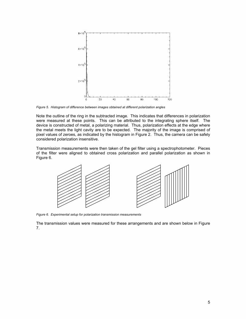
Figure 5. Histogram of difference between images obtained at different polarization angles Note the outline of the ring in the subtracted image. This indicates that differences in polarization were measured at these points. This can be attributed to the integrating sphere itself. The device is constructed of metal, a polarizing material. Thus, polarization effects at the edge where the metal meets the light cavity are to be expected. The majority of the image is comprised of pixel values of zeroes, as indicated by the histogram in Figure 2. Thus, the camera can be safely considered polarization insensitive. Transmission measurements were then taken of the gel filter using a spectrophotometer. Pieces of the filter were aligned to obtained cross polarization and parallel polarization as shown in Figure 6.

Figure 6. Experimental setup for polarization transmission measurements The transmission values were measured for these arrangements and are shown below in Figure 7.

5

0.01

0.1

1

10

100

300 400 500 600 700 800

Wavelength (nm)

Tran

smis

sion

Gel ParallelGel Perpendicular

Figure 7. Transmission plots of gel filter Note the poor efficiency in the red channel of the cross polarization plot. To neglect the effects of transmission leakage, only the green channel was used for image acquisition. Nikon was contacted to obtain the spectral sensitivity of the Coolpix 995 green channel. Due to proprietary license, this data could not be released. As such, the green channel was assumed to range from 500 to 600 nm. The transmission of the camera mounted filter was also measured. The transmission plot is shown in Figure 8.

0

10

20

30

40

50

60

350 400 450 500 550 600 650 700 750 800

Wavelength (nm)

Perc

ent T

rans

mis

sion

Figure 8. Transmission plot of camera linear filter

6

The experimentally obtained Stokes parameters in Equation 2 assume ideal transmission. As shown in Figure 8, the camera linear filter does not exhibit ideal transmission of 50%. As only the green channel was used during image acquisition, the transmission values across 500 to 600 nm were averaged and determined to be 38%. Implementation of this transmission correction factor can be found in the Appendix portion of this report. Both manmade and natural objects were used for the target scene as shown below in Figure 9.

Sand Ball

MILSPEC Paint on Aluminum

Medium Sandpaper

Cotton

Fine

Figure 9. Contents of scene.

A large block of aluminusilicon wafer were used isand, pieces of mediumrepresent natural objectsthe brushed aluminum annot commonly found in understood material. Theellipsometer. These mea

BrushedAluminum

Sandpaper Silicon Wafer

m coated with MILSPEC paint, a piece of brushed aluminum, and a n the scene to represent manmade objects. A hemisphere coated with grade sandpaper, cotton, and fine grade sandpaper were used to . Note that in this color image, there is no enhanced contrast between d cotton. Indeed, they appear fairly similar. Though silicon surfaces are the environment, this item was included because it is a very well index of refraction and extinction coefficients were measured using an

surements are included in Figure 10.

7

0

1

2

3

4

5

6

7

8

300 350 400 450 500 550 600 650 700 750 800

Wavelength (nm)

Ref

ract

ive

Inde

x (n

) & E

xtin

ctio

n C

oeffi

cien

t (k)

nk

Figure 10. Plots of refractive index and extinction coefficient for silicon The items in the scene were placed on a piece of rough wood. An area of the wood piece was sectioned off, textured with fine sand, and covered with a matte black paint to create a quasi-Lambertian surface. A utility was included in DIRSIG to create spherical objects. As such, the sand ball was included in the target scene. The hemisphere needed to be coated with a substance for which some material properties could be approximated. Fine sand was selected to cover the hemisphere and assumed to share similar material properties with the fine grade sandpaper. It is important to note that the material properties for the majority of the contents of the scene are virtually unknown. The MILSPEC aluminum and silicon wafer are fairly well characterized, but very little is known about the remaining items in the scene. In order to provide some experimental data for the DIRSIG bi-directional reflectance distribution function (BRDF) models, exiting spectral radiance was measured off of the MILSPEC aluminum block for several different angles as shown in Figure 11.

8

Figure 11. Measured BRDF angles Results The light source and camera geometry of the first set of pictures is illustrated below in Figure 12.

Figure 12. Light and camera geometry for first set of DoLP images The results of the DoLP calculations for this particular light source and camera geometry are shown below in Figure 13.

9

Figure 13. DoLP image for: (clockwise from upper left corner) Light 45° polarized, Horizontally polarized, Vertically polarized, and Unpolarized Note that the silicon wafer is not visible in any of these DoLP images. This is due to insufficient diffuse reflection off of the silicon surface during image capture. As such, this portion of the image presented as noise. This effect occurred in any area of the images where there was no or low signal. For purposes of presentation, the DoLP images shown in this report have been thresholded and processed to remove areas of high noise. The light source and camera geometry of the second set of pictures is illustrated below in Figure 14.

Figure 14. Light and camera geometry for second set of DoLP images

10

The results of the DoLP calculations for this particular light source and camera geometry are shown below in Figure 15.

Figure 15. DoLP image for: (clockwise from upper left corner) Light 45° polarized, Horizontally polarized, Vertically polarized, and Unpolarized The light source and camera geometry of the third set of pictures is illustrated below in Figure 16.

Figure 16. Light and camera geometry for third set of DoLP images The results of the DoLP calculations for this particular light source and camera geometry are shown below in Figure 17.

11

Figure 17. DoLP image for: (clockwise from upper left corner) Light 45° polarized, Horizontally polarized, Vertically polarized, and Unpolarized The mean DoLP value of each facet, except the silicon wafer and sand ball, in all of the images presented in Figures 13, 15, and 17 are reported below in Tables 1, 2, and 3. Mean DoLP values of the sand ball are not included because of a high degree of variation in signal. This is expected due to the curvature of the surface of the hemisphere.

Material

Light Source 45° Polarized

Light Source Horizontally Polarized

Light Source Vertically Polarized

Light Source Unpolarized

MILSPEC 0.74 ± 0.03 0.31 ± 0.05 0.64 ± 0.03 0.20 ± 0.03 Aluminum 0.92 ± 0.02 0.40 ± 0.06 0.82 ± 0.03 0.36 ± 0.07

Fine Sandpaper 0.48 ± 0.04 0.09 ± 0.04 0.35 ± 0.02 0.25 ± 0.06 Medium Sandpaper 0.42 ± 0.04 0.09 ± 0.04 0.33 ± 0.03 0.23 ± 0.06

Cotton 0.37 ± 0.05 0.21 ± 0.06 0.30 ± 0.03 0.27 ± 0.08

Table 1. DoLP values for first set of images

Material Light Source 45° Polarized

Light Source Horizontally Polarized

Light Source Vertically Polarized

Light Source Unpolarized

MILSPEC 0.20 ± 0.03 0.52 ± 0.04 0.16 ± 0.04 0.33 ± 0.03 Aluminum 0.38 ± 0.03 0.74 ± 0.03 0.35 ± 0.04 0.30 ± 0.04

Fine Sandpaper 0.11 ± 0.02 0.28 ± 0.03 0.07 ± 0.02 0.30 ± 0.02 Medium Sandpaper 0.13 ± 0.02 0.36 ± 0.05 0.08 ± 0.02 0.30 ± 0.03

Cotton 0.08 ± 0.03 0.19 ± 0.06 0.08 ± 0.03 0.30 ± 0.03

Table 2. DoLP values for second set of images

12

Material

Light Source 45° Polarized

Light Source Horizontally Polarized

Light Source Vertically Polarized

Light Source Unpolarized

MILSPEC 0.45 ± 0.03 0.67 ± 0.04 0.14 ± 0.05 0.16 ± 0.04 Aluminum 0.63 ± 0.03 0.82 ± 0.04 0.27 ± 0.03 0.14 ± 0.03

Fine Sandpaper 0.20 ± 0.02 0.28 ± 0.03 0.03 ± 0.01 0.06 ± 0.02 Medium Sandpaper 0.27 ± 0.03 0.38 ± 0.04 0.04 ± 0.02 0.10 ± 0.04

Cotton 0.18 ± 0.03 0.26 ± 0.04 0.10 ± 0.02 0.11 ± 0.04

Table 3. DoLP values for third set of images Discussion By inspection of both the DoLP images and tables, there appears to be enhanced contrast between the natural and manmade objects. Both the MILSPEC aluminum block and brushed aluminum are brighter in the DoLP images than the pieces of sandpaper and cotton. One feature of particular interest is the enhanced contrast between the brushed aluminum and cotton present in the images where the light is polarized. Remember, however, there was little contrast between the aluminum and cotton in the unpolarized color image in Figure 9. Also note that the contrast between the aluminum and cotton is not obvious, particularly in the unpolarized DoLP in Figure 15. Figure 18 below is a plot of contrast, defined as the ratio of brushed aluminum DoLP to cotton DoLP for each set of images.

0

0.5

1

1.5

2

2.5

3

3.5

4

4.5

5

Set 01 Set 02 Set 03 Set 01 Set 02 Set 03 Set 01 Set 02 Set 03 Set 01 Set 02 Set 03

Rat

io o

f Alu

min

um to

Cot

ton

DoLP: Light VerticalDoLP: Light HorizontalDoLP: Light 45 DegDoLP: Light Unpolarized

Figure 187. Plot of aluminum to cotton DoLP for each set of images As shown in the plot above, the mean DoLP of aluminum is at least twice that of the cotton for the majority of DoLP images where the light source was polarized. Clearly, this effect does not hold for the DoLP images where the light source was unpolarized.

13

Conclusion Data for the polarized DIRSIG module was gathered, and experimental Degree of Linear Polarization values for a selection of manmade and natural objects were calculated. The results of this experiment indicated that some metal surfaces, such as brushed aluminum, exhibit considerably higher polarization signatures than some natural surfaces, such as cotton, under particular illumination and viewing conditions. Specifically, enhanced contrast was apparent between the brushed aluminum and cotton under polarized lighting. Evidently the material properties of aluminum are such that it emits polarized light when illuminated with a polarized source even for diffuse reflection. This concept can be further investigated when material property data for brushed aluminum is available. The DoLP’s for unpolarized light sources for each set of images did not show marked contrast between the manmade and natural items in the scene. The data from this experiment suggests that using multiple polarization bands is not useful for imaging with unpolarized light. The conditions under which this experiment was conducted were simulated in DIRSIG as shown below in Figure 19.

Figure 19. Left: DoLP when light is unpolarized for first set of images. Right: DIRSIG simulation A very low resolution DIRSIG simulation is shown in above in Figure 19. The DIRSIG material data bases at the time of this test were not populated with calibrated polarization sensitive bidirectional reflectances. As a result, the simulation in Figure 19 is only indicative of the ability of DIRSIG to render polarization sensitive results. Full validation of the polarization module must await the availability of well characterized materials.

14

References

1 Bragg, W., The Universe of Light, Dover Publications, New York, pp.164-198, 1959.

2 Hecht, E., Optics, Addison Wesley, New York, pp. 319-371 1998. 3 Meyers, J., “Proposal of Modeling Polarimetric Imaging using DIRSIG”, Unpublished, 2001.

15

Appendix

This is IDL code to calculate DoLP. ; ************************************************************************************ ; ; This program performs degree of linear polarization (DoLP) calculations. ; ; ************************************************************************************ ; ************************************************************************************ ; ; Read in tiff images and convert from byte to float. ; ; cam_45 = image for camera polarization state -> 45 deg-ly polarized ; cam_hor = image for camera polarization state -> horizontally polarized ; cam_unpol = image for camera polarization state -> unpolarized ; ; ************************************************************************************ cam_45 = DIALOG_PICKFILE(TITLE = 'Select a 45 degree polarized image.') cam_45 = READ_TIFF(cam_45) cam_45 = FLOAT(cam_45) cam_hor = DIALOG_PICKFILE(TITLE = 'Select a horizontally polarized image.') cam_hor = READ_TIFF(cam_hor) cam_hor = FLOAT(cam_hor) cam_unpol = DIALOG_PICKFILE(TITLE = 'Select a vertically polarized image.') cam_unpol = READ_TIFF(cam_unpol) cam_unpol = FLOAT(cam_unpol) ; ************************************************************************************ ; ; Define exposure corrections. These numerical values for these variables are ; obtained during the image acquisition process. ; ; exp_45 = exposure for image for camera polarization state -> 45 deg-ly polarized ; exp_hor = exposure for image for camera polarization state -> horizontally polarized ; exp_unpol = exposure for image for camera polarization state -> unpolarized ; ; ************************************************************************************ exp_45 = 0.0 READ, exp_45, PROMPT = 'Enter exposure value for 45 degree polarized image: ' exp_hor = 0.0 READ, exp_hor, PROMPT = 'Enter exposure value for horizontally polarized image: ' exp_unpol = 0.0 READ, exp_unpol, PROMPT = 'Enter exposure value for vertically polarized image: ' ; ************************************************************************************ ; ; Define transmission correction for I0. The equations calculating Stokes parameters ; assumes perfect transmission, 0.5. The transmission correction term can be ; experimentally obtained by measuring transmission of the camera filter and averaging ; the transmission values across the green channel (wavelengths: 500-600 nm). ; ; ************************************************************************************

16

trans_correction = 0.0 READ, trans_correction, PROMPT = 'Enter transmission correction: ' ; ************************************************************************************ ; ; Implement the exposure and transmission corrections. ; ; ************************************************************************************ I0 = cam_unpol * trans_correction / exp_unpol I1 = cam_hor /exp_hor I2 = cam_45 / exp_45 ; ************************************************************************************ ; ; Calculate Stokes parameters for DoLP. ; ; ************************************************************************************ S0 = 2 * I0 S1 = 2 * (I1 - I0) S2 = 2 * (I2 - I0) ; ************************************************************************************ ; ; Obtain dimensions of input image. ; ; ************************************************************************************ s = SIZE(S0) ; ************************************************************************************ ; ; Create an empty array to dump DoLP calculations into. ; ; ************************************************************************************ DOLP = MAKE_ARRAY(s[1], s[2], /DOUBLE ) ; ************************************************************************************ ; ; num setups up the numerator of the DoLP equation outside of the for loop for faster ; computation time. ; ; ************************************************************************************ num = SQRT((S1 ^ 2.0) + (S2 ^ 2.0)) FOR i = 0, s[1]-1 DO BEGIN FOR j = 0, s[2]-1 DO BEGIN IF S0[i,j] GT 0.0 THEN BEGIN DOLP[i,j] = num[i,j] / S0[i,j] ; if there is signal, proceed ENDIF ELSE BEGIN ; if no signal, set pixel to 0 DOLP[i,j] = 0.0 ENDELSE ENDFOR ENDFOR

17

; ************************************************************************************ ; ; Resize image for visualization purposes as it is a huge array! ; ; ************************************************************************************ image = REBIN(DOLP, s[1], s[2]) ; ************************************************************************************ ; ; TV resized DOLP. ; ; ************************************************************************************ WINDOW, 1, TITLE = "DOLP ", XSIZE = s[1], YSIZE = s[2] & TV, 255 * image, /ORDER ; ************************************************************************************ ; ; The variable noise is a reality check for the DoLP calculations. DoLP is ; theoretically supposed to range from 0 to 1. If there is low or no signal in any of ; the pixels in S0, the DoLP calculations for said pixels will approach infinity. ; This effect is expected to occur where there is low signal, such as shadows. This ; effect should not occur in targets of interest in the scene (except if the target of ; interest has no diffuse reflection, such as a mirror). Thus, the variable noise is ; a quick visual reality check to determine where the noise in the DoLP images occur. ; ; ************************************************************************************ noise = image LT 1.0 ; ************************************************************************************ ; ; TV noise and check to see where the black pixels occurs and ensure they correspond ; to areas of low or no signal. ; ; ************************************************************************************ WINDOW, 2, TITLE = "Noise", XSIZE = s[1], YSIZE = s[2] & TVSCL, noise, /ORDER END; end program

18