ROOTSOFPOLYNOMMLS

by

KHA W INN SENG

Project submitted in partial fulfillment of the requirements for the degree

ofMaster of Sciences (Teaching ofMathematics)

June 2007

847818

rb {-G<A-HI p~q ~itS

~1-

i; '

ACKNOWLEDGEMENTS

First of all, I would like to thank God for his grace, mercy and the opportunity

he gave me to further my study. This project would not have been made possible

without the assistance of many individual whom I am very grateful. It is a great pleasure

for me to acknowledge those many people who have influenced me in my thoughts and

contributed to my knowledge.

I would like to take this opportunity to record my heartfelt gratitude-especially

to my supervisor, Prof. 0ng Boon Hua for her valuable help, guidance, understanding,

advice and encouragement in the cQurse ()f writing this proje<?t. I would_ also like to

record my sincere thanks to the staff of the School of Mathematical Sciences for

extending their help in the preparation of amenities.

My appreciation also goes to all my friends and those who have in one way or

another helped, encouraged and motivated me during the progression of my project.

Last but not least, I would like to dedicate this project to my parents, wife and

sons as a small acknowledgement of their unfailing love and endless support.

11

ACKNOWLEDGEMENTS

TABLE OF CONTENTS

LISTS OF TABLES

LIST OF FIGURES

ABSTRAK

ABSTRACT

CHAPTER I

CHAPTER2

CHAPTER3

TABLE OF CONTENTS

11

lll

v

V1

vii

viii

INTRODUCTION

1.1 Introduction of the Roots of Polynomials 1

1.2 Objectives of the Project

1.3 Scope of the Project

THE FUNDAMENTAL THEOREM OF ALGEBRA

QUADRATIC EQUATIONS

3.1 Completing the Square

3.2 The Method of Geometry

3.3 Factorization

iii

4

5

7

13

15

16

CHAPTER4 CUBIC EQUATIONS

4.1 Cardano' s Method 24

CHAPTERS NUMERICAL ESTIMATION FOR THE ROOTS OF NONLINEAR FUNCTIONS

5.1 The Bisection Method 35

5.2 Newton's Method 38

5.3 The Secant Method 48

5.4 Hybrid Algorithm with Fast Global Convergence 53

CHAPTER6 APPLICATIONS OF THE ROOTS OF POLYNOMIALS

6.1 Application in the Field of Engineering 59

6.2 Application in the Field of Business and 62 Economics

6.4 Application in the Field of Physics 64

6.5 Application in the field of Design and Art 66

CHAPTER7 CONCLUSION 70

REFERENCES 73

IV

I

I I l

LIST OFT ABLES

TABLE TITLE

5.1 Bisection method applied to p(x) = x 7 + 9x

5 -13x -17

5.2 Hybrid algorithm applied to f ( x) = 20

x -1

19x

v

PAGE

37

58

LIST OF FIGURES

Vl

PUNCA POLINOMIAL

ABSTRAK

Punca polinomial mempunyai pelbagai applikasi dalam kehidupan kita. Ia timbul

bukan sahaja dalam bidang sains dan kejuruteraan malah dalam bidang perniagaan dan

ekonomi dan juga dalam bidang rekaan dan seni.

Dalam projek ini, kami mengkaji Teorem Asasi Aljabar dan pembuktiannya

untuk mengesahkan kewujudan ·punca polinomial. Kami memerikan kaedah pencarian

penyelesaian tepat bagi persamaan kuadratik dengan melengkapkan kuasa dua ata~

formula kuadratik, dengan geometri dan pemfaktoran. Algoritma Cardano dikaji untuk

mendapatkan penyelesaian tepat bagi persamaan kubik. dan pembahagian sintesis untuk

memfaktorkan polinomial, khas bagi polinomial berdarjah tinggi. Kami membincang

pendekatan berangka bagi punca hampiran polinomial dengan kaedah pembahagian

duasama, kaedah Newton, kaedah secant dan algoritma hibrid. Kepentingan punca

diilustrasik.an dengan beberapa aplik.asi.

Vll

' I I ~ 'I

! ABSTRACT

Roots of polynomials have diverse applications in real life. It arises not only in

the fields of science and engineering but also in the field of business and economics and

even in the field of design and art.

In this project, we study the Fundamental Theorem of Algebra and present its

proof to confirm the existence of roots of polynomials. We describe methods for finding

the exact solutions of quadratic equations by completing· the square or the quadratic

formula, by geometry and factorization. Cardano's. algorithm is studied to obtain the

exact solutions for cubic equations and synthetic division for factorizing polynomials, in

particular for polynomials of higher degree. We discuss the numerical approach for the

approximate roots of polynomials by bisection method, Newton's method, secant

method and the hybrid algorithm. The importance of the roots is illustrated by some

examples.

Vlll

.• ~.

CHAPTER1

INTRODUCTION

I

I 1.1 Introduction of the Roots of Polynomials

f A polynomial is built from terms called monomials, each of which consists of a

coefficient multiplied by one or more variables. It is the sum of a finite number of

monomials. In this project, we are considering only polynomials in one variable and

with real numbers as coefficients. The variable may have a non-negative integer

exponent that is the degree of that variable .in that monomial.

The polynomial

3x2 -5x+4

1 consists of three monomials, the first of degree two, the second of degree one and the

! third of degree zero. The degree of a polynomial is the largest degree of any one term. A

' 1 polynomial of degree zero is called a constant, of degree one is said to be linear, of

I I degree two is said to be quadratic, of degree three is said to be cubic. A polynomial of

I I I

I

degree n in x has the general representation

where a; , 0 ::;; i ::;; n , are real numbers and an -:;:. 0 .

A polynomial function is a function defined by evaluating a polynomial. For

example, the function f defined by

1

I

I

f(x)=2x 3 +6x+2

is a polynomial function. Evaluation of a polynomial consists of assigning a number to

the variable and carrying out the indicated multiplications and additions.

A polynomial equation is an equation in which a polynomial is set equal to zero.

The degree of the polynomial equation is the highest exponent of the variable in the

equation. For example,

3x2 +4x-5 = 0

and

are respectively polynomial equations of degree 2 and 20.

A real or complex number x0 is a solution to the polynomial equation P(x) = 0

if it satisfies the equation. The solutions to the polynomial equation P(x) = 0 are called

the roots of the polynomial P(x) and they are the zeroes of the polynomial function and

thus the x - intercepts of its graph if they are real.

Some polynomials, such as f(x) = x 2 + 1, do not have any roots among the real

numbers. If, however, the set of allowed solutions is expanded to the complex numbers,

then every non-constant polynomial has at least one distinct root. This follows from the

Fundamental Theorem of Algebra. However, in this project we are emphasising more on

the real roots of the polynomial.

Formulas for the roots of polynomials up to a degree of2 have been known since

ancient times. On clay tablets dated between 1800 BC and 1600 BC, the ancient

2

Babylonians left the earliest evidence of the discovery of quadratic equations, and also

gave early methods for solving them. The Indian mathematician Baudhayana who wrote

a Sulba Sutra in ancient India about 8th century BC first used quadratic equations of the

form ax 2 = c and ax 2 + b = c and also gave methods for solving them.

Babylonian mathematicians from about 400 BC and Chinese mathematicians

from about 200 BC used the method of completing the square to solve quadratic

equations with positive roots, but did not have a general formula. Euclid produced a

more abstract geometrical method around 300 BC.

In the early 16th century, the Italian mathematician Scipione del Ferro (1456-

1526) found a method for solving cubic equations of the form x 3 + mx = n, where m, n

are integers. Del Ferro kept his achievement a secret until just before his death, when he

told his student Antonio Fiore about it.

In 1530, Niccolo Tartaglia (1500 - 1557) received questions in the form

'

I '

x 3 + mx = n, for which he had worked out a general method, won the contest between

he and Antonio Fiore.

Later, Tartaglia was persuaded by Gerolamo Cardano (1501 -1576) to reveal his

secret for solving cubic equations. Tartaglia did so only on the condition that Cardano

would never reveal it. A few years later, Cardano learned about Ferro's prior work and

broke the promise by publishing Tartaglia's method in his book Ars Magna ( 1545) with

credit given to Tartaglia.

Approximate solutions to any polynomial equation can be found either by

Newton's method or by one of the many more modem methods of approximating

solutions. Newton's method was described by Isaac Newton (1642 -1727) in De ana~vsi

3

per aequationes numero terminorum infinitas, written in 1669 and published in 1 711 by

William Jones and in De metodis fluxionum et serierum infinitarum, written in 1671,

translated and published as Method of Fluxions in 1736 by John Colson.

Fundamental Theorem of Algebra was conjectured as early as the sixteenth

century. Several incorrect proofs of it were published before Carl Friedrich Gauss (1777

- 1855) found a satisfactory proof in 1797. The proof was mainly geometric, but it had a

topological gap. A rigorous proof was published by Argand in 1806; it was here that, for

the first time, the Fundamental Theorem of Algebra was stated for polynomials with

complex coefficients, rather than just real coefficients. Gauss produced two other proofs

in 1816 and another version of his original proof in 1849.

1.2 Objectives of the Proje~

The objectives of this project are:

• To study some of the theorems and their proofs involved in root-finding

methods

• To study the methods for fmding the exact roots of quadratic and cubic

polynomials

• To study the common numerical methods of root-finding

• To illustrate the importance ofroot-fmding with some applications.

Since this project is about roots of polynomials it is natural to first ask the question,

"How do we know the existence of the roots?" If we are not assured of the existence of

the roots, then this project would be meaningless. Hence, we present and prove the

Fundamental Theorem of Algebra which confirms the existence of the roots of

4

polynomials. In this project we study the methods for exact roots of quadratic and cubic

polynomials. We describe numerical methods for approximate roots of polynomials.

We also illustrate the importance of root-finding with several apllications.

1.3 Scope of the Project

The Scope of this master project includes the introduction of the roots of

polynomials, the Fundamental Theorem of Algebra, the quadratic and cubic equations, .

numerical estimation for the roots of nonlinear polynomials and the applications of the

roots of polynomials.

The discussion begins by introducing the roots of polynomials and a brief history

of quadratic and cubic equations and the Newton's method. In Chapter 2, we state the

Fundamental Theorem of Algebra. The proof of the Fundamental Theorem of Algebra

involves some analysis, at the very least the concept of continuity of real or complex

functions and we prove it by contradiction using Liouville's theorem.

The third chapter is mainly concerned with the quadratic equations and the

various methods of finding its solutions. Synthetic division is also discussed in this

chapter under the heading of factorization. Chapter 4 covers cubic polynomials and

derives the Cardano's formula in fmding the roots.

The next chapter is about the common numerical methods of root-finding,

namely the bisection method, Newton's method and secant method. It also discusses the

hybrid algorithm with fast global convergence. Chapter 6 focuses on the applications of

the roots of polynomials.

5

The last chapter is the conclusion of the project about the roots of polynomials.

6

CHAPTER2

THE FUNDAMENTAL THEOREM OF ALGEBRA

As this project concerns the roots of polynomial equations, we shall begin by

discussing what is probably the most important result in the theory of equations, i.e. the

Fundamental Theorem of Algebra (Beaumont and Pierce, 1963).

Theorem 2.1 (The Fundamental Theorem of Algebra)

If P is a non-zero complex polynomial of degree greater or equal to 1, then P has at

least one root inC, where C denotes the complex plane.

This theorem was conjectured as early as the sixteenth century. Several incorrect

proofs of it were published before Gauss found a satisfactory proof in 1797. Gauss

ultimately gave five different proofs of the Fundamental Theorem of Algebra, each of

which introduced new ideas and methods, which have greatly influenced the

development of mathematics.

Proving the theorem algebraically is quite difficult and it involves tools such as

field, irreducible polynomial, subring and others, which are not covered in this project.

However, we shall prove this theorem using Liouville's theorem (Marsden, 1973).

Before proving Liouville's theorem, we shall state Cauchy's Inequalities, which will be

7

used in the proof. We recall that a complex function f is said to be analytic on A cC

if f is complex differentiable at each z0 eA. The phrase "analytic at z0 " means

complex differentiable on a neighborhood of z0 • A function that is defmed and analytic

on the whole plane C is said to be entire.

Theorem 2.2 (Cauchy's Inequalities)

Let f be an analytic function on a region A in C and let r be a' circle with radius

rand center z0

that lies in A. Assume that the disk { z eCII z- z0 I< r} also lies in A.

Suppose that !f(x)! ~ M for all z on y. Then, for any k = 0, 1, 2, ... ,

Theorem 2.3 (Liouville's Theorem)

If f is entire and bounded for all z e C, then f is constant.

Proof:

Since f is bounded, there is an M > 0 such that lf(z)l ~ M for any z eC. For any

a eC, Cauchy's inequality gives

lf'(a)!~ M r

for any r > 0 . By letting r ~ oo , we get

f '(a)= 0.

8

I I

I

l

Thus f ' ( z) = 0 for all z E C and therefore the function f is a constant function on C.

After stating Liouville's theorem and proving it, we are now able to prove the

Fundamental Theorem of Algebra. We shall prove by contradiction by assuming that the

polynomial p has no zero in C. We then prove that f(z) = -1- is a bounded entire

p(z)

function and use Liouville's theorem to get a contradiction

( cs.usm.my/~vravilmss30 1.html).

Proof: (The Fundamental Theorem of Algebra)

Let

be a polynomial of degree n when n ~ 1. Then an ::1= 0. Note that as lzl ~ oo, then

lp(z)l ~ oo. This follows as

and when I z I ~ oo , I zn I ~ oo and an + a~-I + ... + :~ ~ I an I·

1 Assume that p( z) :to 0 for any z E C. We are going to show that f(z) = -- IS

p(z)

bounded. Let

9

For 1 z 1 ~ 2nA ~ 1, we have

and therefore by applying the triangle inequality

By writing

weseethat,for I z l~2nA~1,

2

Hence 1 I ,;; I I 2 for all I z I <! 2nA . Since p( z) ;, 0 and it is continuous for p(z)j an (2nAY

any z e C, the function - 1- is continuous in C, and therefore on the compact set p(z)

I z I ::::; 2nA, it is bounded, say by M . Thus we have for all z E C,

10

IP:z~,; max {M, I a. I ~2nA)"}.

Thus _!_ is a bounded entire function and hence by Liouville's Theorem, it reduces to p(z)

a constant function, which is a contradiction. This proves that there is at least one root

for p(z).

Corollary 2.1

Any polynomial equation p(z) = 0 of degree n > 0 has exactly n roots in C.

Proof:

We prove the result by mathematical induction. Clearly any polynomial of degree 1 has

exactly one root in C. Assume that the result is true for any polynomial of degree m .

Let p(z) be a polynomial of degree m + 1. By the Fundamental Theorem of Algebra,

there is a root for p( z) and denote the root by a. Then (z -a) is a factor of p( z) and

hence p(z) = (z- a )q(z) where q(z) is a polynomial of degree m and hence it has

exactly m roots. Thus p(z) has exactly m + 1 roots.

The general form of the degree n equation is:

(2.1)

From Corollary 2.1, we know that any polynomial equation of the degree n as in (2.1)

always has n solutions in C. In particular cases, some or all of these n solutions could

11

be equal to one another. Though the coefficients a; may be real numbers, the solutions

could be real or complex numbers.

12

cJIAPTER3

QUADRATIC EQUATIONS

A quadratic equation is a polynomial equation of the second degree. The general

form is ax2 + bx + c = 0, where a¢ 0. a, b, and care coefficients which are real.

Quadratic equations are called quadratus in Latin, which means 'squares'. In the

leading term the variable is squared.

There are a few methods of finding the solutions of a quadratic equation

ax2 +-bx + c = 0 or equivalently the roots of a polynomial ax2

+ bx + c . They are

discussed below.

(http://faculty.ed.umuc.edu/--swalsh!Math%20Articles/Quadratic%20Equations.html)

3.1 Completing the Square

This method makes use of the algebraic identity: x2 + 2xy + y2

= (x + y Y .

Dividing the quadratic equation

ax2 +bx+c = 0 (3.1)

by a gives

2 b c x +-x+-=0.

a a

13

Its equivalent is

2 b c X +-X=--. (3.2)

a a

To complete the square is to find some constant k such that

2 b 2 2 X +-X+ k == X + 2xy + y .

a

For this equation to hold it must be the case that y = !!_ and k = y2

, thus k = b

2

2 • 2a 4a

Adding this constant to both sides of the equation (3.2) produces

The left is now a perfect square of x + .!!._ . This gives 2a

(. b )

2 b2 -4ac

. x+ 2a = 4a2 - •

Taking the square root of both sides yields

x+_!_ = ± .Jb2 -4ac.

2a 2a

So

-b±.Jb2 -4ac X=------

2a

which is also known as quadratic formula.

(3.3)

From the formula (3.3), the term underneath the square root sign b2

- 4ac IS

called the discriminant of the quadratic equation.

14

cases:

The discriminant determines the number and nature of the roots. There are three

i) If it is positive, there are two distinct roots, both of which are real

numbers.

ii) If it is zero, there is exactly one root, and that root is a real number.

Sometimes, it is called a double root, its value is x = _!!__. 2a

iii) If it is negative, there are no real roots but there two distinct complex

roots. They are

-b ·(~4ac-b2 ) d -b ·(~4ac-b2 ) x=-+1 an x=--1 ----2a 2a 2a 2a

where i is the imaginary unit.

Thus, a quadratic equation (3.1) with real coefficient has two, not necessarily

distinct roots, which may be real or complex, given by the quadratic formula (3.3), the

symbol ' ± ' indicates that both

-b+~b2 -4ac -b-.Jb2 -4ac X= and X=------

2a 2a

are solutions.

3.2 The Method of Geometry

Consider the quadratic equation

ax2 +bx+c = 0.

It is easy to see that the solutions are the intercept of x-axis of the quadratic function

f(x) = ax 2 + bx + c when these solutions are real.

15

ila<o ...

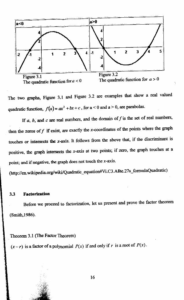
Figure 3.1 The quadratic function for a < 0

Figure 3.2 The quadratic function for a > 0

The two graphs, Figure 3.1 and Figure 3.2 are examples that show a real valued

quadratic function, f(x) = ax2 + bx + c , for a < 0 and a > 0, are parabolas.

If a, b, and c are real numbers, and the domain off is the set of real numbers,

then the zeros off if exist, are exactly the x-coordinates of the points where the graph

touches or intersects the x-axis. It follows from the above that, if the discriminant is

positive, the graph intersects the x-axis at two points; if zero, the graph touches at a

point; and if negative, the graph does not touch the x-axis.

(http://en. wikipedia.orglwiki!Quadratic _ equation#Vi.C3 .A8te.27s _ formulaQuadratic)

3.3 Factorization

Before we proceed to factorization, let us present and prove the factor theorem

(Smith, 1986).

Theorem 3.1 (The Factor Theorem)

( x - r) is a factor of a polynomial P( x) if and only if r is a root of P( x) .

16

Proof:

Suppose (x- r) is a factor of P(x) then P(r) will have the factor (r- r), which is 0.

This will make P(r) = 0 . This means that r is a root.

Conversely, if r is a root of P(x), then P(r) = 0. But according to the remainder

theorem, P(r) = 0 means that upon dividing P(x) by (x- r) , the remainder is 0.

Therefore (x- r) is a factor of P(x).

By the Fundamental Theorem of Algebra, the factor theorem allows us to conclude:

P(x) =a (x- rn)(x- rn_1) ••• (x- r2 ) (x-r1)

for some a, rl' ,2' ... rn E C.

To solve a quadratic equation by factoring, we may do the following simple steps:

(i) first we must make sure it is in standard form, ax2

+ bx + c = 0

(ii) then we must factor the left side if possible

(iii) lastly we set each of the two factors equal to zero and solve the equations we

get to find the solutions to the equation.

Example 3.1

Solve the equation

Solution: Factoring yields the equation

(2x -1)(x + 1) = 0 .

17

Hence, we have

2x -1 = 0 or x + 1 = 0

which yield

1 x=- or x=-1.

2

1 Thus x = - or x = -1 are the roots of the equation 2x 2 + x -1 = 0. ' 2

Note that not all polynomials can be factored into real factors. For example the

polynomial,

2x2 +3x-1,

cannot be factored easily. ThJ.IS, to find its root we have to tise either by quadratic

formula or the method of completing the square. The quadratic formula or completing

the square are always applicable in solving quadratic equations and the solutions are

exact. However, when we actually use these methods we generally have to approximate

the numbers involved, especially when extracting square roots.

Now we are going to show a method of factorizing polynomials, in particular for

polynomials of higher degree, by synthetic division (Smith, 1986).

Synthetic division is a shortcut method for dividing a polynomial by a linear

factor of the form x - s . It can be used in place of the standard long division algorithm.

This method reduces the polynomial and the linear factor into a set of numeric values.

After these values are processed, the resulting set of numeric outputs is used to construct

the polynomial quotient and the polynomial remainder.

Suppose that

18

(3.4)

is a given polynomial, r is an exact solution of P(x). Then P(r) = 0. One way to test

whether s is indeed a root of P(x) is to see whether x- s divides P(x). We therefore

write

P(x) = Q(x) + b0 (s) x-s x-s

where Q(x) is said to be the quotient which must be a polynomial of degree n -1 and

b0

is said to be the remainder which. is a constant with respect to x but of course

depends on s, as the notation implies. If s is an exact root then b0 will be zero. These

statements and the following presentation are valid whether s is real or complex

number.

We have

P(x) = (x-s)Q(x) + b0 (s) (3.5)

for all numbers s . We need to determine the coefficients of the degree n - 1 polynomial

Q(x) and the remainder b0

, given the coefficients of P(x). To determine them

synthetically, let

Then

P(x) = (x- s)Q(x) + b0

19

should be identical to (3.4).

For polynomials to be equal as functions of x, every corresponding coefficient must be

the same. Setting corresponding coefficients of (3.4) and (3.6) equal to one another, we

get

To use these equations, we need to solve them for the {bk}, one at a time, starting with

b = a . We therefore write the equations in the form n n

This set of n + 1 equations can be compactly written as

(3.7)

with k = n, n -1, ... , 1, 0 . Here bn+t is assumed to be zero.

Equation (3.7) can be viewed as a finite iteration process. The first n numbers

obtained are the coefficients of the quotient polynomial Q(x), in order, starting with the

highest degree term and the last number is the remainder b0 • It also follows from

equation (3.5) that

b0 = P(s)

so this process can be used to evaluate a polynomial. In particular, if b0 = 0 then s is a

The process of synthetic division is performed efficiently using the following

,!pattern:

20

an an-I an-2 a2 at ao

+ sbn sbn-1 sb3 sb2 sb1

bn bn-1 bn-2 b2 b, I b0

We shall illustrate how synthetic division works by looking at two examples.

Example 3.2:

Find the roots of 15x4 + x3 - 52x2 + 20x + 16.

Solution:

Let us try x = 1 , i.e. put s = 1.

15 1 -52 20 16

s=1 + 15 16 -36 -16 -

15 16 -36 -16 1 o

This gives a zero remainder, so x = 1 is a root, which means that (x -1) is a factor.

Since we divide a linear factor out of (x -1), this means that the quotient is a cubic:

15x3 + 16x2 - 36x -16.

Thus we need to find another zero before we can apply the quadratic formula. We will

try x=-2:

15 16 -36 -16

s=-2 + -30 28 16

15 -14 -8 lo Since we get a zero remainder, x = -2 is a root, so (x + 2) is a factor. This leaves us

with the quadratic :

15x2 -14x-8.

By factoring, we obtain

21

(3x-4)(5x+2).

Then the fully factored form is:

15x4 + x3- 52x2 + 20x + 16 = (x -l)(x +2)(3x-4)(5x + 2).

4 -2 The roots are x = 1, - 2, -, -.

3 5

Example 3.3:

Given that (2- i) is a root of x 5 - 6x4 + llx3

- x 2 -14x + 5, fully solve the equation

Solution:

Since (2 - i) is a given root, we shall use synthetic division and divide out (2 - i) :

1 -6 11 -1 -14 5

s=2-i + 2-i -9+2i 6+2i 12-i -5

1 -4-i 2+2i 5+2i -2-i 1 0

Since (2 - i) is a root, then its complex conjugate (2 + i) is also a root of the equation.

1 -4-i 2+2i 5+2i -2-i

s =2+i + 2+i -4-2i -4-2i 2+i

1 -2 -2 1 I 0

This leaves us with a cubic:

Letustry x=-1:

1 -2 -2 1

s =-1 + -1 3 -1

1 -3 1 1 o

22

Now we get a quadratic:

Thus by using quadratic formula, we get

3±.J5 x=

2

Hence, all the roots of x 5 - 6x3 + llx3

- x2

-14x + 5 are

X= 2±i, 3±../5

2 -1.

Synthetic division is useful for factorizing polynomials of higher degree to find

the exact roots. The process to evaluate the polynomial for a right root is very tedious

and time consuming. However, we can quicken the process with the tools such as

rational roots test and Descartes' rule of signs, which we are _not going to explore here

(http://www.purplemath.com/modules/synthdiv4.html).

23

CHAPTER4

CUBIC EQUATIONS

A cubic equation is a polynomial equation in which the highest occurring power

the variable is the third power. The general form may be written as:

O.JX3 + 0.2J!- + O.tX + 0.0 = 0.

coefficients a.o, ... , 0.3 are real numbers. We will always assume that a3 is non-zero

it is a quadratic or lower degree equation).

:nhr1n<T a cubic equation amounts to finding the roots of a cubic function.

Cardano's Method

first cubic equations to be solved were those of the form:

x 3 +px+q=0 (4.1)

• The key to solving this equation is to note that the apparent more complicated equation:

w6 +Bw3 +C=O

in fact easy to solve because it is a quadratic in w3

:

( w 3)

2 + Bw3 + C = 0 .

would like to convert the original equation, x 3 + px + q = 0, into this easily solved

form by using a simple substitution. This might appear to be impossible until we realise

24