Root Locus Method. Root Locus Motivation To satisfy transient performance requirements, it may be...
33
Root Locus Method
-
Upload
mae-stewart -
Category
Documents
-
view
223 -
download
0
Transcript of Root Locus Method. Root Locus Motivation To satisfy transient performance requirements, it may be...
Root Locus Method
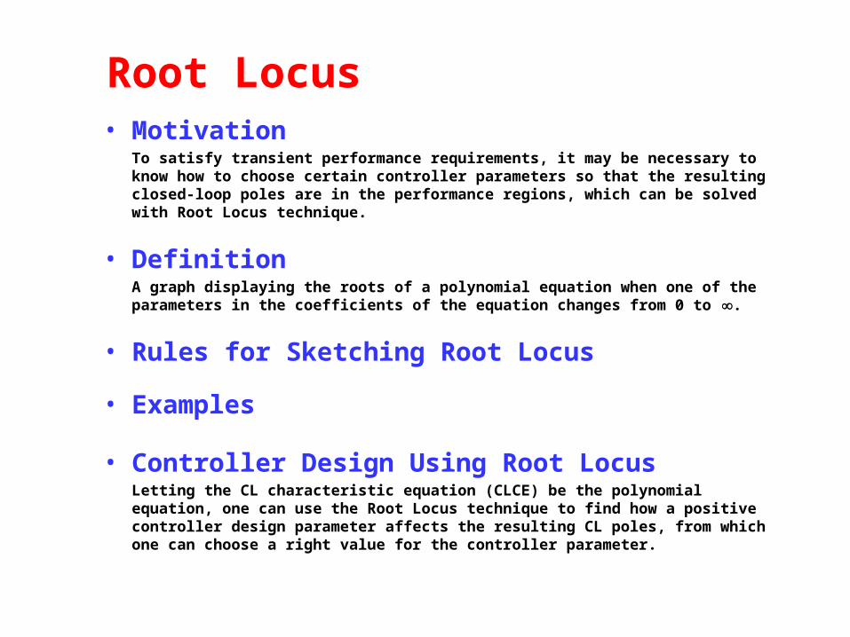
Root Locus• Motivation
To satisfy transient performance requirements, it may be necessary to know how to choose certain controller parameters so that the resulting closed-loop poles are in the performance regions, which can be solved with Root Locus technique.
• DefinitionA graph displaying the roots of a polynomial equation when one of the parameters in the coefficients of the equation changes from 0 to .
• Rules for Sketching Root Locus
• Examples
• Controller Design Using Root LocusLetting the CL characteristic equation (CLCE) be the polynomial equation, one can use the Root Locus technique to find how a positive controller design parameter affects the resulting CL poles, from which one can choose a right value for the controller parameter.
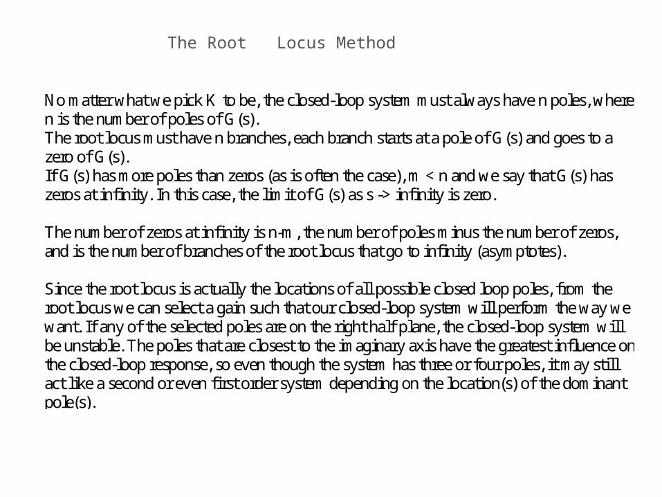
No matter what we pick K to be, the closed-loop system must always have n poles, where n is the number of poles of G(s). The root locus must have n branches, each branch starts at a pole of G(s) and goes to a zero of G(s). If G(s) has more poles than zeros (as is often the case), m < n and we say that G(s) has zeros at infinity. In this case, the limit of G(s) as s -> infinity is zero. The number of zeros at infinity is n-m, the number of poles minus the number of zeros, and is the number of branches of the root locus that go to infinity (asymptotes). Since the root locus is actually the locations of all possible closed loop poles, from the root locus we can select a gain such that our closed-loop system will perform the way we want. If any of the selected poles are on the right half plane, the closed-loop system will be unstable. The poles that are closest to the imaginary axis have the greatest influence on the closed-loop response, so even though the system has three or four poles, it may still act like a second or even first order system depending on the location(s) of the dominant pole(s).
The Root Locus Method
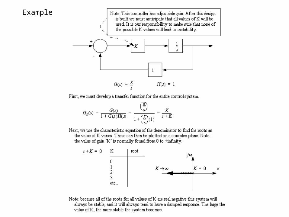
Example
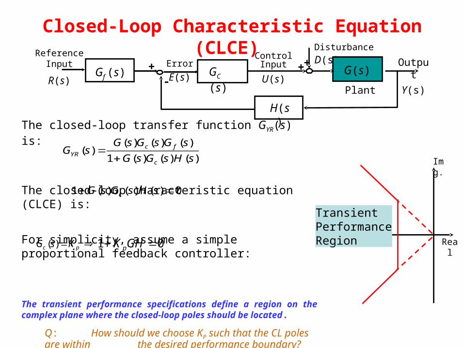
Closed-Loop Characteristic Equation (CLCE)
( )c pG s K Real
Img.
GC (s)
H(s)
+
Reference Input
R(s)
Error
E(s)++ Output
Y(s)
Disturbance
D(s)
Plant
G(s)Control Input
U(s)Gf (s)
The closed-loop transfer function GYR(s) is:
The closed-loop characteristic equation (CLCE) is:
For simplicity, assume a simple proportional feedback controller:
The transient performance specifications define a region on the complex plane where the closed-loop poles should be located.
Q: How should we choose KP such that the CL poles are within the desired performance boundary?
( ) ( ) ( )( )
1 ( ) ( ) ( )c f
YRc
G s G s G sG s
G s G s H s
1 ( ) ( ) ( ) 0cG s G s H s
01 GHK p
TransientPerformanceRegion
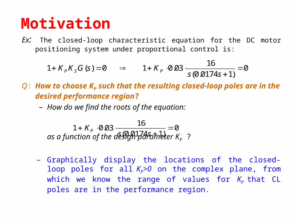
Ex: The closed-loop characteristic equation for the DC motor positioning system under proportional control is:
Q: How to choose KP such that the resulting closed-loop poles are in the desired performance region?
– How do we find the roots of the equation:
as a function of the design parameter KP ?
– Graphically display the locations of the closed-loop poles for all KP>0 on the complex plane, from which we know the range of values for KP that CL poles are in the performance region.
Motivation
161 ( ) 0 1 0.03 0
(0.0174 1)P S PK K G s Ks s
1 0 0316
0 0174 10
K
s sP .( . )
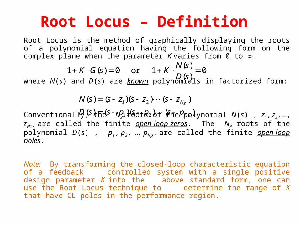
Root Locus is the method of graphically displaying the roots of a polynomial equation having the following form on the complex plane when the parameter K varies from 0 to :
where N(s) and D(s) are known polynomials in factorized form:
Conventionally, the NZ roots of the polynomial N(s) , z1 , z2 , …, zNz , are called the finite open-loop zeros. The NP roots of the polynomial D(s) , p1 , p2 , …, pNp , are called the finite open-loop poles.
Note: By transforming the closed-loop characteristic equation of a feedback controlled system with a single positive design parameter K into the above standard form, one can use the Root Locus technique to determine the range of K that have CL poles in the performance
region.
Root Locus – Definition
1 0 1 0 K G s KN s
D s( )
( )
( ) or
1 2
1 2
( ) ( )( ) ( )
( ) ( )( ) ( )Z
P
N
N
N s s z s z s z
D s s p s p s p
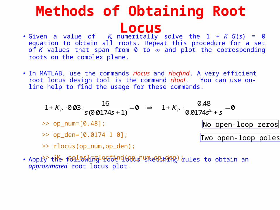
• Given a value of K, numerically solve the 1 + K G(s) = 0 equation to obtain all roots. Repeat this procedure for a set of K values that span from 0 to and plot the corresponding roots on the complex plane.
• In MATLAB, use the commands rlocus and rlocfind. A very efficient root locus design tool is the command rltool. You can use on-line help to find the usage for these commands.
• Apply the following root locus sketching rules to obtain an approximated root locus plot.
Methods of Obtaining Root Locus
1 0 0316
0 0174 10 1
0
0 017402
K
s sK
s sP P.( . )
.48
.
>> op_num=[0.48];
>> op_den=[0.0174 1 0];
>> rlocus(op_num,op_den);
>> [K, poles]=rlocfind(op_num,op_den);
No open-loop zeros
Two open-loop poles
Root Locus Sketching Rules
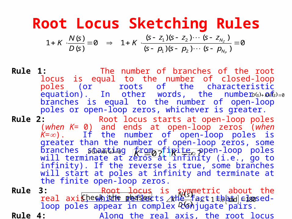
Rule 1: The number of branches of the root locus is equal to the number of closed-loop poles (or roots of the characteristic equation). In other words, the number of branches is equal to the number of open-loop poles or open-loop zeros, whichever is greater.
Rule 2: Root locus starts at open-loop poles (when K= 0) and ends at open-loop zeros (when K=). If the number of open-loop poles is greater than the number of open-loop zeros, some branches starting from finite open-loop poles will terminate at zeros at infinity (i.e., go to infinity). If the reverse is true, some branches will start at poles at infinity and terminate at the finite open-loop zeros.
Rule 3: Root locus is symmetric about the real axis, which reflects the fact that closed-loop poles appear in complex conjugate pairs.
Rule 4: Along the real axis, the root locus includes all segments that are to the left of an odd number of finite real open-loop poles and zeros.
0 sKNsD
1 0 1 01 2
1 2
KN s
D sK
s z s z s z
s p s p s pN
N
Z
P
( )
( )
( )( ) ( )
( )( ) ( )
?K
0 sKNsD
Check the phases 1 rad 180
N sK
D s
0?K
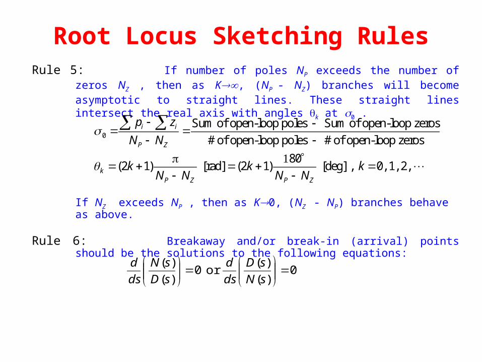
Root Locus Sketching RulesRule 5: If number of poles NP exceeds the number of zeros NZ , then as K,
(NP - NZ) branches will become asymptotic to straight lines. These straight lines intersect the real axis with angles k at 0 .
If NZ exceeds NP , then as K0, (NZ - NP) branches behave as above.
Rule 6: Breakaway and/or break-in (arrival) points should be the solutions to the following equations:
0
Sum of open-loop poles Sum of open-loop zeros
# of open-loop poles # of open-loop zeros
80(2 1) [rad] (2 1) [deg] , 0, 1, 2,
i i
P Z
kP Z P Z
p z
N N
k k kN N N N
0)(
)(or 0
)(
)(
sN
sD
ds
d
sD
sN
ds
d
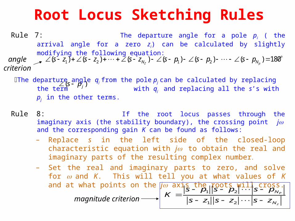
Root Locus Sketching RulesRule 7: The departure angle for a pole pi ( the arrival angle for a zero zi) can be
calculated by slightly modifying the following equation:
The departure angle qj from the pole pj can be calculated by replacing the term with qj and replacing all the s’s with pj in the other terms.
Rule 8: If the root locus passes through the imaginary axis (the stability boundary), the crossing point j and the corresponding gain K can be found as follows:
– Replace s in the left side of the closed-loop characteristic equation with j to obtain the real and imaginary parts of the resulting complex number
– Set the real and imaginary parts to zero, and solve for and K. This will tell you at what values of K and at what points on the j axis the roots will cross.
( ) ( ) ( ) ( ) ( ) ( )s z s z s z s p s p s pN NZ p1 2 1 2 180
( )js p
1 2
1 2
P
z
N
N
s p s p s pK
s z s z s z
magnitude criterion
angle criterio
n
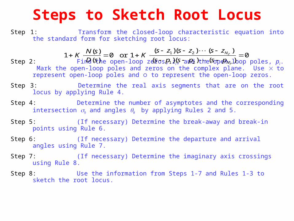
Steps to Sketch Root LocusStep 1: Transform the closed-loop characteristic equation into the standard form for
sketching root locus:
Step 2: Find the open-loop zeros, zi, and the open-loop poles, pi. Mark the open-loop poles and zeros on the complex plane. Use to represent open-loop poles and to represent the open-loop zeros.
Step 3: Determine the real axis segments that are on the root locus by applying Rule 4.
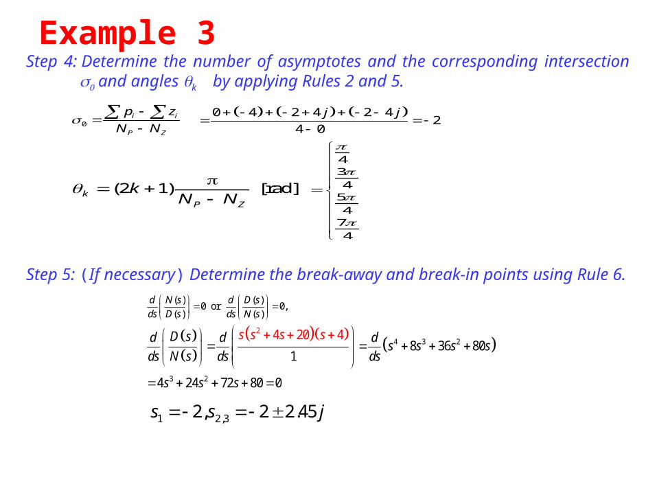
Step 4: Determine the number of asymptotes and the corresponding intersection and angles kby applying Rules 2 and 5.
Step 5: (If necessary) Determine the break-away and break-in points using Rule 6.
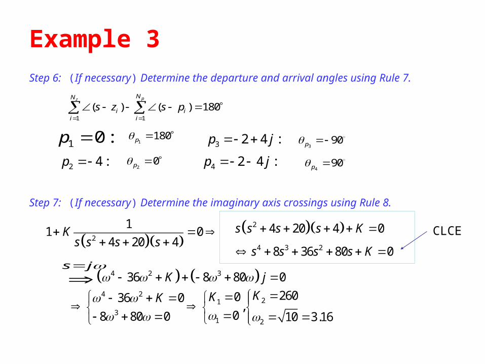
Step 6: (If necessary) Determine the departure and arrival angles using Rule 7.
Step 7: (If necessary) Determine the imaginary axis crossings using Rule 8.
Step 8: Use the information from Steps 1-7 and Rules 1-3 to sketch the root locus.
1 0 1 01 2
1 2
KN s
D sK
s z s z s z
s p s p s pN
N
Z
P
( )
( )
( )( ) ( )
( )( ) ( ) or
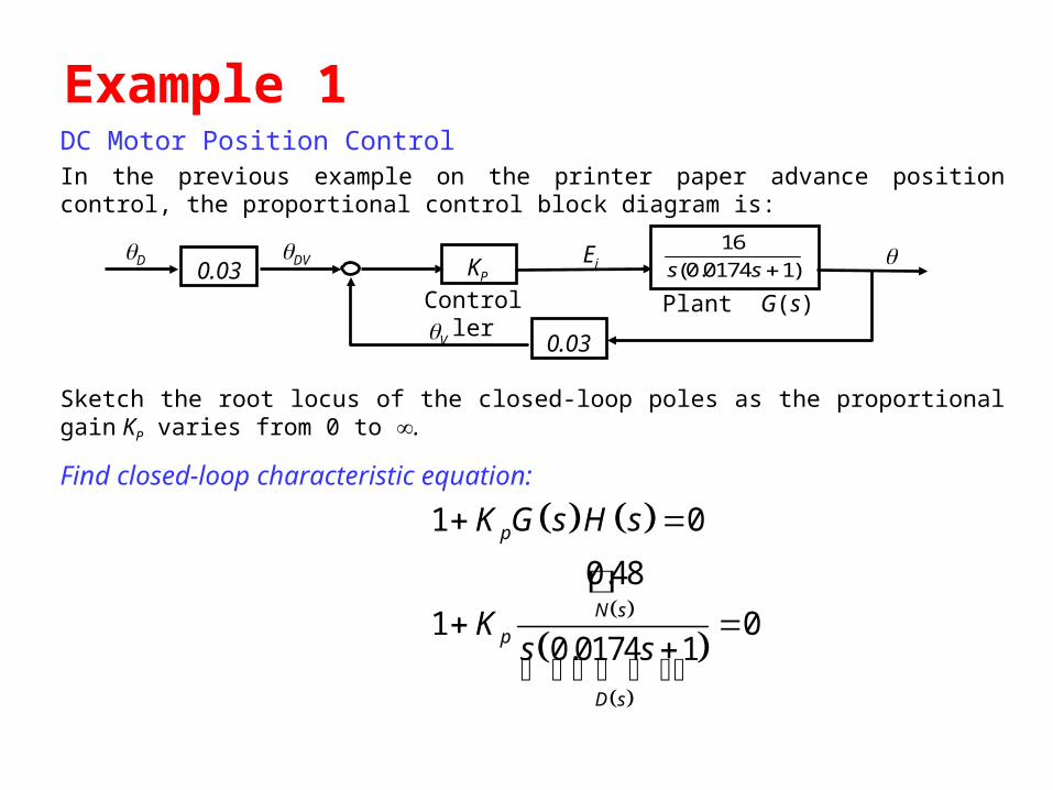
Example 1DC Motor Position ControlIn the previous example on the printer paper advance position control, the proportional control block diagram is:
Sketch the root locus of the closed-loop poles as the proportional gain KP varies from 0 to .
Find closed-loop characteristic equation:
Ei
Plant G(s)Controller
DV16
0 0174 1s s( . )KP0.03
V
D
0.03
1 0
0.48
1 00.0174 1
p
N s
p
D s
K G s H s
Ks s
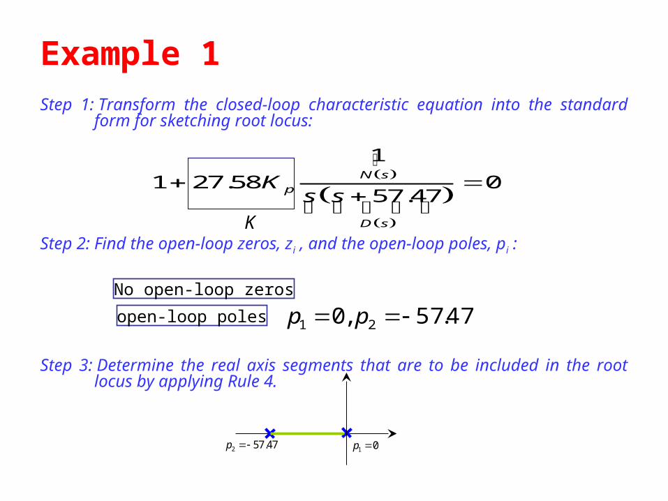
Example 1Step 1: Transform the closed-loop characteristic equation into the standard form for
sketching root locus:
Step 2: Find the open-loop zeros, zi , and the open-loop poles, pi :
Step 3: Determine the real axis segments that are to be included in the root locus by applying Rule 4.
47.57,0 21 ppNo open-loop zeros
open-loop poles
1
1 27.58 057.47
N s
p
D s
Ks s
1 0p 2 57.47p
K
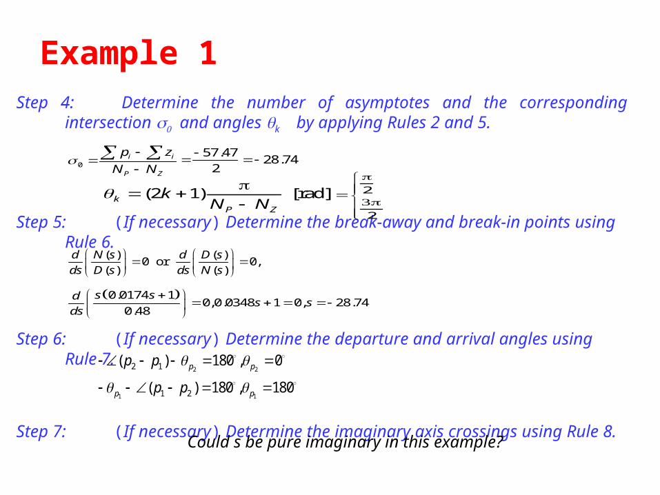
Example 1Step 4:Determine the number of asymptotes and the corresponding intersection
and angles kby applying Rules 2 and 5.
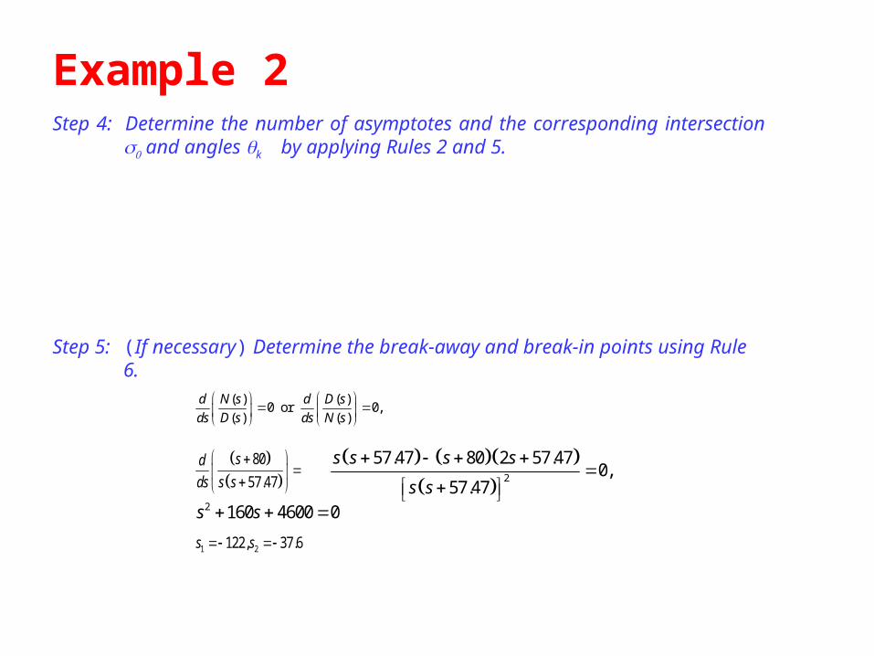
Step 5:(If necessary) Determine the break-away and break-in points using Rule 6.
Step 6:(If necessary) Determine the departure and arrival angles using Rule 7.
Step 7:(If necessary) Determine the imaginary axis crossings using Rule 8.
(2 1) [rad]kP Z
kN N
( ) ( )0 or 0,
( ) ( )
d N s d D s
ds D s ds N s
2 2
1 1
2 1
1 2
( ) 180 , 0
( ) 180 , 180
p p
p p
p p
p p
Could s be pure imaginary in this example?
2
2
0i i
P Z
p z
N N
57.47
28.742
0.0174 10,0.0348 1 0, 28.74
0.48
s sds s
ds
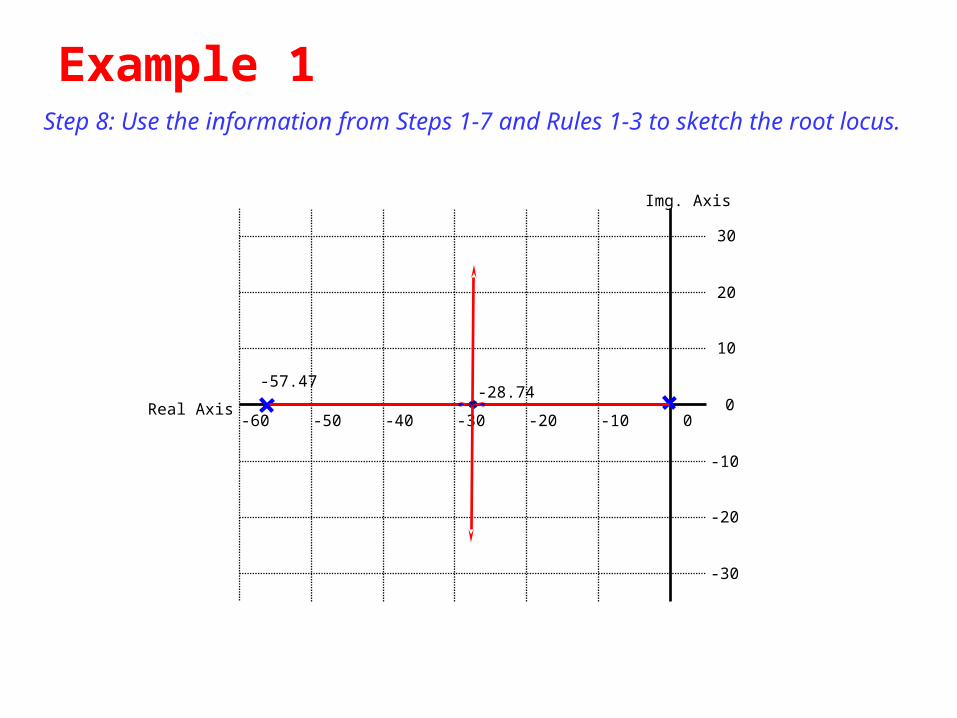
Example 1Step 8: Use the information from Steps 1-7 and Rules 1-3 to sketch the root locus.
-60 -50 -40 -30 -20 -10 0Real Axis
-30
-20
-10
0
10
20
30
Img. Axis
-57.47-28.74
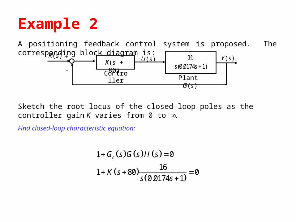
Example 2A positioning feedback control system is proposed. The corresponding block diagram is:
Sketch the root locus of the closed-loop poles as the controller gain K varies from 0 to .
Find closed-loop characteristic equation:
Y(s)U(s)
Plant G(s)Controller
R(s) 16
0 0174 1s s( . )K(s + 80)+
1 0
161 80 0
0.0174 1
cG s G s H s
K ss s
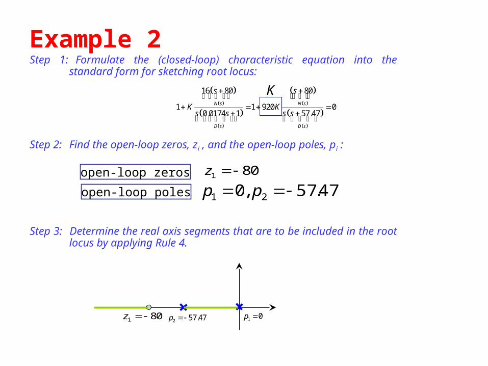
Example 2Step 1: Formulate the (closed-loop) characteristic equation into the standard form
for sketching root locus:
Step 2: Find the open-loop zeros, zi , and the open-loop poles, pi :
Step 3: Determine the real axis segments that are to be included in the root locus by applying Rule 4.
16 80 80
1 1 920 00.0174 1 57.47
N s N s
D s D s
s s
K Ks s s s
47.57,0 21 ppopen-loop zeros
open-loop poles
1 80z
1 0p 2 57.47p 1 80z
K
Example 2Step 4: Determine the number of asymptotes and the corresponding intersection and
angles kby applying Rules 2 and 5.
Step 5: (If necessary) Determine the break-away and break-in points using Rule 6.
( ) ( )0 or 0,
( ) ( )
d N s d D s
ds D s ds N s
2
57.47 80 2 57.470,
57.47
s s s s
s s
80
57.47
sd
ds s s
1 2122, 37.6s s
2 160 4600 0s s
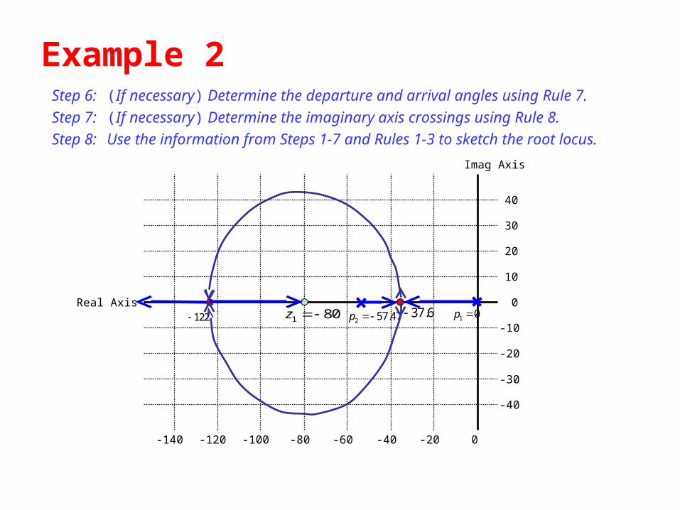
Example 2Step 6: (If necessary) Determine the departure and arrival angles using Rule 7.
Step 7: (If necessary) Determine the imaginary axis crossings using Rule 8.
Step 8: Use the information from Steps 1-7 and Rules 1-3 to sketch the root locus.
122
-140 -120 -100 -80 -60 -40 -20 0
-40
-30
-20
-10
0
10
20
30
40
Real Axis
Imag Axis
1 0p 2 57.47p 1 80z 37.6
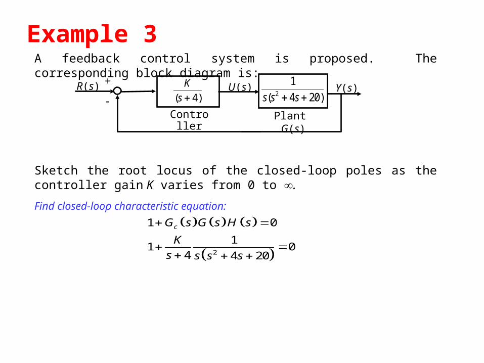
Example 3A feedback control system is proposed. The corresponding block diagram is:
Sketch the root locus of the closed-loop poles as the controller gain K varies from 0 to .
Find closed-loop characteristic equation:
Y(s)U(s)
Plant G(s)Controller
R(s) 1
4 202s s s( ) +
K
s( ) 4
2
1 0
11 0
4 4 20
cG s G s H s
K
s s s s
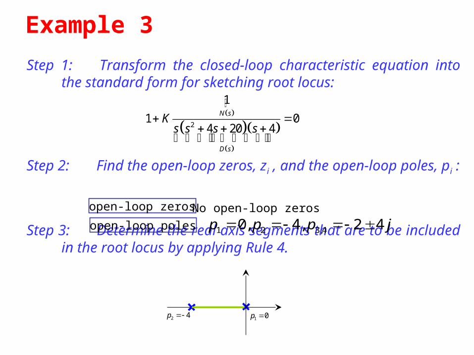
Example 3
Step 1: Transform the closed-loop characteristic equation into the standard form for sketching root locus:
Step 2: Find the open-loop zeros, zi , and the open-loop poles, pi :
Step 3: Determine the real axis segments that are to be included in the root locus by applying Rule 4.
1 2 3,40, 4, 2 4p p p j open-loop zeros
open-loop poles
2
1
1 04 20 4
N s
D s
Ks s s s
No open-loop zeros
1 0p 2 4p
Example 3Step 4: Determine the number of asymptotes and the corresponding intersection and
angles kby applying Rules 2 and 5.
Step 5: (If necessary) Determine the break-away and break-in points using Rule 6.
(2 1) [rad]kP Z
kN N
43
45
47
4
0i i
P Z
p z
N N
0 4 2 4 2 4
24 0
j j
( ) ( )0 or 0,
( ) ( )
d N s d D s
ds D s ds N s
2
4 3 2
3 2
8 36 801
4 24 72 80
4 20 4
0
D sd d ds s s s
ds N s ds d
s s s s
s
s s s
1 2,32, 2 2.45s s j
Example 3
Step 6: (If necessary) Determine the departure and arrival angles using Rule 7.
Step 7: (If necessary) Determine the imaginary axis crossings using Rule 8.
1 1
( ) ( ) 180pz
NN
i ii i
s z s p
3 2 4 :p j
4 2 4 :p j
1180p
1 0 :p
2 4 :p 2
0p
390p
490p
2
11 0
4 20 4K
s s s s
2
4 3 2
4 20 4 0
8 36 80 0
s s s s K
s s s s K
CLCE
s j 4 2 336 8 80 0K j
4 221
31 2
260036 0,
08 80 0 10 3.16
KKK
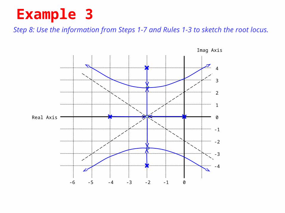
Example 3Step 8: Use the information from Steps 1-7 and Rules 1-3 to sketch the root locus.
-6 -5 -4 -3 -2 -1 0
-4
-3
-2
-1
0
1
2
3
4
Real Axis
Imag Axis
Example 4A feedback control system is proposed. The corresponding block diagram is:
Sketch the root locus of the closed-loop poles as the controller gain K varies from 0 to .
Find closed-loop characteristic equation:
Y(s)U(s)
Plant G(s)Controller
R(s) s s
s s s
2
2
2 101
2 2 26
( )( )K
+
02622
10121
2
2
sss
ssK
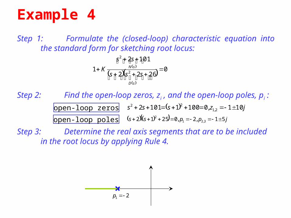
Example 4
Step 1:Formulate the (closed-loop) characteristic equation into the standard form for sketching root locus:
Step 2:Find the open-loop zeros, zi , and the open-loop poles, pi :
Step 3:Determine the real axis segments that are to be included in the root locus by applying Rule 4.
02622
1012
12
2
sD
sN
sss
ss
K
open-loop zeros
open-loop poles
jzsss 101,010011012 2,122
jppss 51,2,02512 3,212
21 p
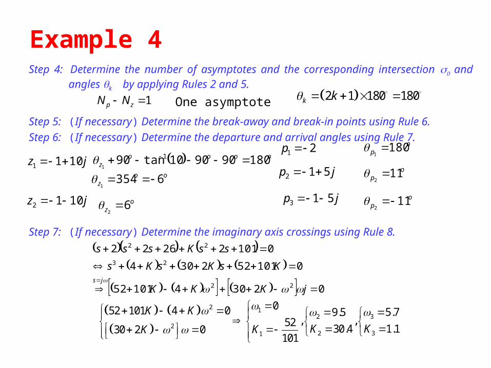
Example 4Step 4: Determine the number of asymptotes and the corresponding intersection and angles
kby applying Rules 2 and 5.
Step 5: (If necessary) Determine the break-away and break-in points using Rule 6.
Step 6: (If necessary) Determine the departure and arrival angles using Rule 7.
Step 7: (If necessary) Determine the imaginary axis crossings using Rule 8.
1 zp NN One asymptote 2 1 180 180k k
jz 1011
jz 1012
21 p
jp 512
jp 513
ooooz 180909010tan90 1
1
ooz 63541
oz 6
2
op 180
1
op 11
2
op 11
2
0230410152
0101522304
010122622
22
23
22
jKKK
KsKsKs
ssKsss
js
2 132
2321
052 101 4 0 5.79.5, ,52
1.130.430 2 0101
K K
KKKK
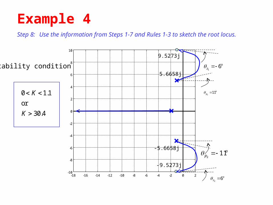
Example 4Step 8: Use the information from Steps 1-7 and Rules 1-3 to sketch the root locus.
0 1.1
or
30.4
K
K
-18 -16 -14 -12 -10 -8 -6 -4 -2 0 2-10
-8
-6
-4
-2
0
2
4
6
8
10
Stability condition
oz 6
2
16o
z
op 11
2
211o
p
9.5273j
-9.5273j
5.6658j
-5.6658j
0 1.1
or
30.4
K
K
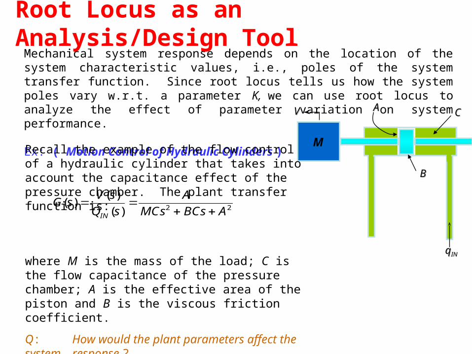
Mechanical system response depends on the location of the system characteristic values, i.e., poles of the system transfer function. Since root locus tells us how the system poles vary w.r.t. a parameter K, we can use root locus to analyze the effect of parameter variation on system performance.
Ex: ( Motion Control of Hydraulic Cylinders )
Root Locus as an Analysis/Design Tool
M
qqININ
Recall the example of the flow control of a hydraulic cylinder that takes into account the capacitance effect of the pressure chamber. The plant transfer function is:
where M is the mass of the load; C is the flow capacitance of the pressure chamber; A is the effective area of the piston and B is the viscous friction coefficient.
Q: How would the plant parameters affect the system response ?
G sV s
Q s
A
MCs BCs AIN
( )( )
( )
2 2
VV CC
BB
AA
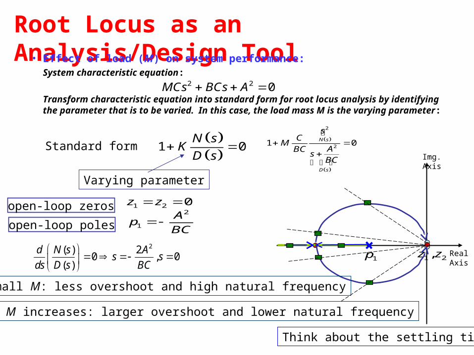
Root Locus as an Analysis/Design Tool• Effect of load (M) on system performance:
System characteristic equation:
Transform characteristic equation into standard form for root locus analysis by identifying the parameter that is to be varied. In this case, the load mass M is the varying parameter:
2
21 0N s
D s
sC
MABC
sBC
MCs BCs A2 2 0
Img. Axis
Real Axis
1 0N s
KD s
Standard form
Varying parameter
2
1
Ap
BC
open-loop zeros
open-loop poles
1 2 0z z
1p 1 2,z z2( ) 2
0 , 0( )
d N s As s
ds D s BC
Small M: less overshoot and high natural frequency
As M increases: larger overshoot and lower natural frequency
Think about the settling time
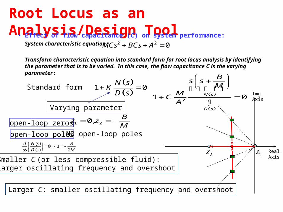
Root Locus as an Analysis/Design Tool• Effect of flow capacitance (C) on system performance:
System characteristic equation:
Transform characteristic equation into standard form for root locus analysis by identifying the parameter that is to be varied. In this case, the flow capacitance C is the varying parameter:
( )0
( ) 2
d N s Bs
ds D s M
MCs BCs A2 2 0
Img. Axis
Real Axis
21 0
1N s
D s
Bs s
MM
CA
1 0N s
KD s
Standard form
Varying parameter
open-loop zeros
open-loop poles
1 20,B
z zM
NO open-loop poles
2z 1zSmaller C (or less compressible fluid):Larger oscillating frequency and overshoot
Larger C: smaller oscillating frequency and overshoot
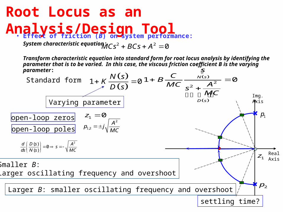
Root Locus as an Analysis/Design Tool• Effect of friction (B) on system performance:
System characteristic equation:
Transform characteristic equation into standard form for root locus analysis by identifying the parameter that is to be varied. In this case, the viscous friction coefficient B is the varying parameter:
2
1,2
Ap j
MC
MCs BCs A2 2 0
Img. Axis
Real Axis
22
1 0N s
D s
sC
BAMC
sMC
1 0N s
KD s
Standard form
Varying parameter
open-loop zeros
open-loop poles
1 0z 1p
2p
1z
2( )0
( )
d D s As
ds N s MC
Smaller B:Larger oscillating frequency and overshoot
Larger B: smaller oscillating frequency and overshoot
settling time?