Roger Wattenhofer @ SOFSEM 2010 –1 TexPoint fonts used in EMF. Read the TexPoint manual before you...
58
Roger Wattenhofer @ SOFSEM 2010 – 1 Theory Meets Practice …it's about TIME!
-
date post
20-Dec-2015 -
Category
Documents
-
view
213 -
download
0
Transcript of Roger Wattenhofer @ SOFSEM 2010 –1 TexPoint fonts used in EMF. Read the TexPoint manual before you...

Roger Wattenhofer @ SOFSEM 2010 – 1
Theory Meets Practice …it's about TIME!

Roger Wattenhofer @ SOFSEM 2010 – 2
Map of Computer Science
theory
[www.confsearch.org]

Roger Wattenhofer @ SOFSEM 2010 – 3
SOFSEM
Zooming in on Theory [www.confsearch.org]

Theory Meets Practice?
FC Practice SC Theory

Why is there so little interaction?
TheoryPractice
Practice is trivial…
Theory is useless…

Roger Wattenhofer @ SOFSEM 2010 – 6
Systems people don’t read theory papers
• Sometimes for good reasons…– unreadable– don’t matter that much (only getting out the last %)– wrong models– theory is lagging behind– bad theory merchandising/branding
– systems papers provide easy to remember acronyms– “On the Locality of Bounded Growth” vs. “Smart Dust”
– good theory comes from surprising places– difficult to keep up with– having hundreds of workshops does not help
• If systems people don’t read theory papers, maybe theory people should build systems themselves?

Roger Wattenhofer @ SOFSEM 2010 – 7
Systems Perspective: Dozer
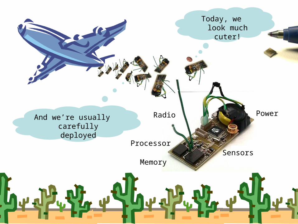
8
Power
Processor
Radio
SensorsMemory
Today, we look much cuter!
And we’re usually carefully deployed

Roger Wattenhofer @ SOFSEM 2010 – 9
A Sensor Network After Deployment
multi-hop communication

Roger Wattenhofer @ SOFSEM 2010 – 10
A Typical Sensor Node: TinyNode 584
• TI MSP430F1611 microcontroller @ 8 MHz
• 10k SRAM, 48k flash (code), 512k serial storage
• 868 MHz Xemics XE1205 multi channel radio
• Up to 115 kbps data rate, 200m outdoor range
[Shockfish SA, The Sensor Network Museum]
Current Draw
Power Consumption
uC sleep with timer on 6.5 uA 0.0195 mW
uC active, radio off 2.1 mA 6.3 mW
uC active, radio idle listening 16 mA 48 mW
uC active, radio TX/RX at +12dBm
62 mA 186 mW
Max. Power (uC active, radio TX/RX at +12dBm + flash write)
76.9 mA 230.7mW

Roger Wattenhofer @ SOFSEM 2010 – 11
Environmental Monitoring (PermaSense)
• Understand global warming in alpine environment
• Harsh environmental conditions• Swiss made (Basel, Zurich)
Go

Example: Dozer
• Up to 10 years of network life-time• Mean energy consumption: 0.066
mW• Operational network in use > 2 years• High availability, reliability (99.999%)
[Burri et al., IPSN 2007]

Roger Wattenhofer @ SOFSEM 2010 – 13
Is Dozer a theory-meets-practice success story?
• Good news– Theory people can develop good systems!– Dozer is to the best of my knowledge more energy-efficient and
reliable than all other published systems protocols… for many years already!
– Sensor network (systems) people write that Dozer is one of the “best sensor network systems papers”, or: “In some sense this is the first paper I'd give someone working on communication in sensor nets, since it nails down how to do it right.”
• Bad news: Dozer does not have an awful lot of theory inside• Ugly news: Dozer v2 has even less theory than Dozer v1• Hope: Still subliminal theory ideas in Dozer?

Roger Wattenhofer @ SOFSEM 2010 – 14
Energy-Efficient Protocol Design
• Communication subsystem is the main energy consumer– Power down radio as much as possible
• Issue is tackled at various layers– MAC – Topology control / clustering– Routing
TinyNode Power Consumption
uC sleep, radio off 0.015 mW
Radio idle, RX, TX 30 – 40 mW
Orchestration of the whole network stackto achieve duty cycles of ~ 0.1%

Roger Wattenhofer @ SOFSEM 2010 – 15
contention window
Dozer System
• Tree based routing towards data sink– No energy wastage due to multiple paths– Current strategy: SPT
• TDMA based link scheduling– Each node has two independent schedules – No global time synchronization
• The parent initiates each TDMA round with a beacon– Enables integration of disconnected nodes– Children tune in to their parent’s schedule
time
beacon
beacon
activation frame
child
parent

Roger Wattenhofer @ SOFSEM 2010 – 16
Dozer System
• Parent decides on its children data upload times– Each interval is divided into upload slots of equal length– Upon connecting each child gets its own slot– Data transmissions are always ack’ed
• No traditional MAC layer– Transmissions happen at exactly predetermined point in time – Collisions are explicitly accepted– Random jitter resolves schedule collisions
time
jitter
slot 1 slot 2 slot n
data transfer
Clock drift, queuing, bootstrap, etc.

Roger Wattenhofer @ SOFSEM 2010 – 17
Dozer in Action

Roger Wattenhofer @ SOFSEM 2010 – 18
Energy Consumption
• Relay node• No scanning
0.28% duty cycle
0.32% duty cycle
• Leaf node• Few neighbors• Short disruptions
scanning
overhearing
updating #children
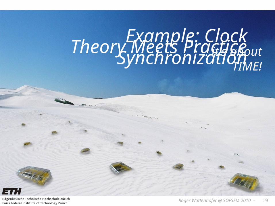
Roger Wattenhofer @ SOFSEM 2010 – 19
Example: Clock Synchronization…it's about TIME!
Theory Meets Practice
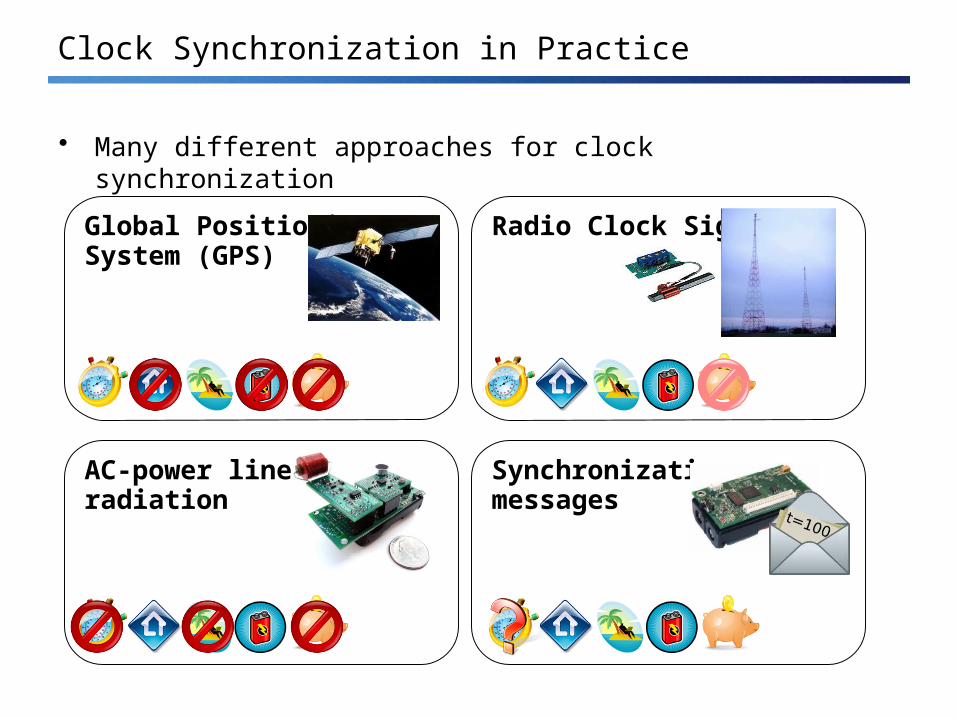
Global Positioning System (GPS)
Radio Clock Signal
AC-power line radiation
Synchronization messages
Clock Synchronization in Practice
• Many different approaches for clock synchronization

Clock Devices in Sensor Nodes
• Structure– External oscillator with a nominal frequency (e.g. 32 kHz or 7.37 MHz)
– Counter register which is incremented with oscillator pulses
– Works also when CPU is in sleep state
32 kHz quartz
Mica2
32 kHz quartz
7.37 MHz quartz
TinyNode

Clock Drift
• Accuracy– Clock drift: random deviation from the nominal rate dependent on power
supply, temperature, etc.
– E.g. TinyNodes have a maximum drift of 30-50 ppm at room temperature
This is a drift of up to 50 μs per second or 0.18s per hour
t
rate
11+²
1-²

Roger Wattenhofer @ SOFSEM 2010 – 23
Sender/Receiver Synchronization
• Round-Trip Time (RTT) based synchronization
• Receiver synchronizes to sender‘s clock• Propagation delay and clock offset can be calculated
22
2
43123412
2314
)t(t+)t(t=
δ))+(t(tδ))+(t(t=θ
)t(t)t(t=δ
t 1
t 2 t 3
t 4
B
A Time accor-ding to A
Request from A
Answer from B
Time accor-ding to B

Roger Wattenhofer @ SOFSEM 2010 – 24
• Problem: Jitter in the message delayVarious sources of errors (deterministic and non-deterministic)
• Solution: Timestamping packets at the MAC layer [Maróti et al.]→ Jitter in the message delay is reduced to a few clock ticks
Messages Experience Jitter in the Delay
SendCmd Access Transmission
Reception Callback
0-100 ms 0-500 ms 1-10 ms
0-100 mstim
estamp
timestamp
t

Roger Wattenhofer @ SOFSEM 2010 – 25
Clock Synchronization in Networks?
• Time, Clocks, and the Ordering of Events in a Distributed SystemL. Lamport, Communications of the ACM, 1978.
• Internet Time Synchronization: The Network Time Protocol (NTP)D. Mills, IEEE Transactions on Communications, 1991
• Reference Broadcast Synchronization (RBS)J. Elson, L. Girod and D. Estrin, OSDI 2002
• Timing-sync Protocol for Sensor Networks (TPSN)S. Ganeriwal, R. Kumar and M. Srivastava, SenSys 2003
• Flooding Time Synchronization Protocol (FTSP)M. Maróti, B. Kusy, G. Simon and Á. Lédeczi, SenSys 2004
• and many more ...
FTSP: State of the art clock sync protocol for networks.

Roger Wattenhofer @ SOFSEM 2010 – 26
Flooding Time Synchronization Protocol (FTSP)
• Each node maintains both a local and a global time• Global time is synchronized to the local time of a reference node
– Node with the smallest id is elected as the reference node• Reference time is flooded through the network periodically
• Timestamping at the MAC Layer is used to compensate for deterministic message delays
• Compensation for clock drift between synchronization messages using a linear regression table
4
6
0
1
2 3
5
7
reference node

Roger Wattenhofer @ SOFSEM 2010 – 27
Best tree for tree-based clock synchronization?
• Finding a good tree for clock synchronization is a tough problem– Spanning tree with small (maximum or average) stretch.
• Example: Grid network, with n = m2 nodes.
• No matter what tree you use, the maximumstretch of the spanning tree will always beat least m (just try on the grid figure right…)
• In general, finding the minimum maxstretch spanning tree is a hard problem, however approximation algorithms exist [Emek, Peleg, 2004].

Roger Wattenhofer @ SOFSEM 2010 – 28
Variants of Clock Synchronization Algorithms
Tree-like Algorithms Distributed Algorithms
e.g. FTSP e.g. GTSP
Bad local skew
All nodes consistently average errors to all neighbors
[Sommer et al., IPSN 2009]

Roger Wattenhofer @ SOFSEM 2010 – 29
FTSP vs. GTSP: Global Skew
• Network synchronization error (global skew)– Pair-wise synchronization error between any two nodes in the network
FTSP (avg: 7.7 μs) GTSP (avg: 14.0 μs)

FTSP vs. GTSP: Local Skew
• Neighbor Synchronization error (local skew)– Pair-wise synchronization error between neighboring nodes
• Synchronization error between two direct neighbors:
FTSP (avg: 15.0 μs) GTSP (avg: 2.8 μs)

Time in (Sensor) Networks
Synchronized clocks are essential for many applications:
Duty-CyclingTDMA
Sensing
Hardware Clock
Localization
Clock Synchronization Protocol
Global Local
LocalLocal
Global
Local
Roger Wattenhofer @ SOFSEM 2010 – 32
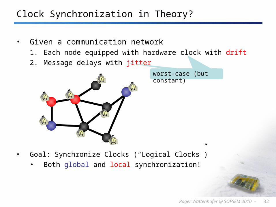
• Given a communication network1. Each node equipped with hardware clock with drift2. Message delays with jitter
• Goal: Synchronize Clocks (“Logical Clocks”)• Both global and local synchronization!
Clock Synchronization in Theory?
worst-case (but constant)

Roger Wattenhofer @ SOFSEM 2010 – 33
• Time (logical clocks) should not be allowed to stand still or jump
• Let’s be more careful (and ambitious):• Logical clocks should always move forward
• Sometimes faster, sometimes slower is OK. • But there should be a minimum and a maximum speed.• As close to correct time as possible!
Time Must Behave!

Formal Model
• Hardware clock Hv(t) = s[0,t] hv(¿) d¿ with clock rate hv(t) 2 [1-²,1+²]
• Logical clock Lv(∙) which increases at rate at least 1 and at most ¯
• Message delays 2 [0,1]
• Employ a synchronization algorithm to update the logical clock according to hardware clock and messages from neighbors
Clock drift ² is typically small, e.g. ² ¼10-4 for a cheap quartz oscillator
Neglect fixed share of delay, normalize jitter
Logical clocks with rate much less than 1 behave differently...
Time is 140 Time is 150
Time is 152
Lv?
Hv

Variants of Clock Synchronization Algorithms
Tree-like Algorithms Distributed Algorithmse.g. FTSP e.g. GTSP
Bad local skew

Roger Wattenhofer @ SOFSEM 2010 – 36
Synchronization Algorithms: An Example (“Amax”)
• Question: How to update the logical clock based on the messages from the neighbors?
• Idea: Minimizing the skew to the fastest neighbor– Set the clock to the maximum clock value received from any neighbor
(if larger than local clock value)– forward new values immediately
• Optimum global skew of about D• Poor local property
– First all messages take 1 time unit…– …then we have a fast message!
Time is D+x Time is D+x
…
Clock value:D+x
Old clock value:D+x-1
Old clock value:x+1
Old clock value:x
Time is D+x
New time is D+xNew time is D+x skew D!
Allow ¯ = 1, i.e. logical clock may jump forward
Fastest Hardware
Clock

Roger Wattenhofer @ SOFSEM 2010 – 37
Local Skew: Overview of Results
1 logD √D D …
Everybody‘s expectation, 10 years ago („solved“)
Lower bound of logD / loglogD[Fan & Lynch, PODC 2004]
All natural algorithms [Locher et al., DISC 2006]
Blocking algorithm
Kappa algorithm[Lenzen et al., FOCS 2008]
Tight lower bound[Lenzen et al., PODC 2009]
Dynamic Networks![Kuhn et al., SPAA 2009]
together[JACM 2010]

Roger Wattenhofer @ SOFSEM 2010 – 38
Enforcing Clock Skew
• Messages between two neighboring nodes may be fast in one direction and slow in the other, or vice versa.
• A constant skew between neighbors may be „hidden“.
• In a path, the global skew may be in the order of D/2.
2 3 4 5 6 7
2 3 4 5 6 7
2 3 4 5 6 7
2 3 4 5 6 7
2 3 4 5 6 7
2 3 4 5 6 7
u
v
Roger Wattenhofer @ SOFSEM 2010 – 39
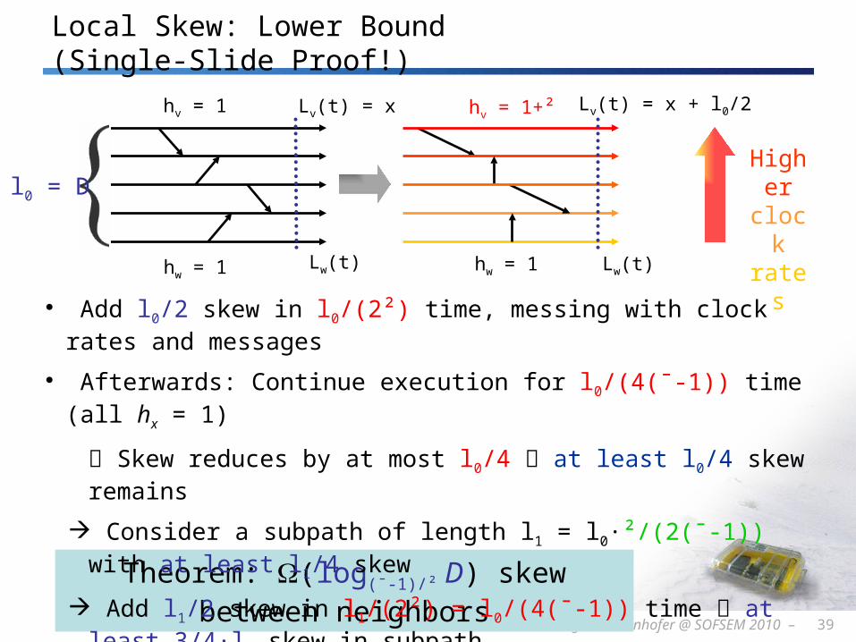
Local Skew: Lower Bound (Single-Slide Proof!)
Theorem: (log(¯-1)/² D) skew between neighbors
• Add l0/2 skew in l0/(2²) time, messing with clock rates and messages
• Afterwards: Continue execution for l0/(4(¯-1)) time (all hx = 1)
Skew reduces by at most l0/4 at least l0/4 skew remains
Consider a subpath of length l1 = l0·²/(2(¯-1)) with at least l1/4 skew
Add l1/2 skew in l1/(2²) = l0/(4(¯-1)) time at least 3/4·l1 skew in subpath
• Repeat this trick (+½,-¼,+½,-¼,…) log2(¯-1)/² D times
Higher clock rates
l0 = D
Lv(t) = x + l0/2
Lw(t)
Lv(t) = x
Lw(t)
hv = 1+²hv = 1
hw = 1 hw = 1

Roger Wattenhofer @ SOFSEM 2010 – 40
• Surprisingly, up to small constants, the (log(¯-1)/² D) lower bound can be matched with clock rates 2 [1,¯] (tough part, not in this talk)
• We get the following picture [Lenzen et al., PODC 2009]:
max rate ¯ 1+² 1+£(²) 1+√² 2 large
local skew 1 £(log D) £(log1/² D) £(log1/² D) £(log1/² D)
Local Skew: Upper Bound
... because too large clock rates will amplify
the clock drift ².
We can have both smooth and
accurate clocks!

Roger Wattenhofer @ SOFSEM 2010 – 41
• Surprisingly, up to small constants, the (log(¯-1)/² D) lower bound can be matched with clock rates 2 [1,¯] (tough part, not in this talk)
• We get the following picture [Lenzen et al., PODC 2009]:
• In practice, we usually have 1/² ¼ 104 > D. In other words, our initial intuition of a constant local skew was not entirely wrong!
max rate ¯ 1+² 1+£(²) 1+√² 2 large
local skew 1 £(log D) £(log1/² D) £(log1/² D) £(log1/² D)
Local Skew: Upper Bound
... because too large clock rates will amplify
the clock drift ².
We can have both smooth and
accurate clocks!

Clock Synchronization vs. Car Coordination
• In the future cars may travel at high speed despite a tiny safety distance, thanks to advanced sensors and communication

Clock Synchronization vs. Car Coordination
• In the future cars may travel at high speed despite a tiny safety distance, thanks to advanced sensors and communication
• How fast & close can you drive?
• Answer possibly related to clock synchronization – clock drift ↔ cars cannot control speed perfectly– message jitter ↔ sensors or communication between cars not perfect

Is Our Theory Practical?!?…it's about TIME!
Example: Clock Synchronization

One Big Difference Between Theory and Practice, Usually!
TheoryPractice
Worst Case Analysis!
Physical Reality...

As we have seen FTSP does have a local skew problem
But it’s not all that bad…
However, tests revealed another (severe!) problem:
FTSP does not scale: Globalskew grows exponentiallywith network size…
„Industry Standard“ FTSP in Practice
FTSP (avg: 15.0 μs)

How does the network diameter affect synchronization errors?
Examples for sensor networks with large diameterBridge, road or pipeline monitoring
Deployment at Golden Gate Bridge with 46 hops[Kim et al., IPSN 07]
Why?
0 1 2 3 4 ... d

Roger Wattenhofer @ SOFSEM 2010 – 48
Multi-hop Clock Synchronization
• Nodes forward their current estimate of the reference clock– Each synchronization beacon is affected by a random jitter J
• Sum of the jitter grows with the square-root of the distance– stddev(J1 + J2 + J3 + J4 + J5 + ... Jd) = √d×stddev(J)
• This is bad but does not explain exponential behavior of FTSP…
• In addition FTSP uses linear regression to compensate for clock drift– Jitter is amplified before it is sent to the next hop!– Amplification leads to exponential behavior…
0 1 2 3 4 ... d

Simulation of FTSP with regression tables of different sizes(k = 2, 8, 32)
Linear Regression (FTSP)
Lo
g S
cale
!

1) Remove self-amplifying of synchronization error2) Send fast synchronization pulses through the network
- Speed-up the initialization phase- Faster adaptation to changes in temperature or network topology
The PulseSync Protocol
t
01234
t
01234
FTSPExpected time
= D·B/2
PulseSyncExpected time
= D·tpulse
[Lenzen et al., SenSys 2009]

Testbed setup- 20 Crossbow Mica2 sensor nodes- PulseSync implemented in TinyOS 2.1- FTSP from TinyOS 2.1
Network topology- Single-hop setup, basestation- Virtual network topology (white-list)- Acknowledgments for time sync beacons
Evaluation
0 1 2 3 4 20... Probe beacon

Global Clock Skew• Maximum synchronization error between any two nodes
Experimental Results
Synchronization Error FTSP PulseSync
Average (t>2000s) 23.96 µs 4.44 µs
Maximum (t>2000s) 249 µs 38 µs
FTSP PulseSync
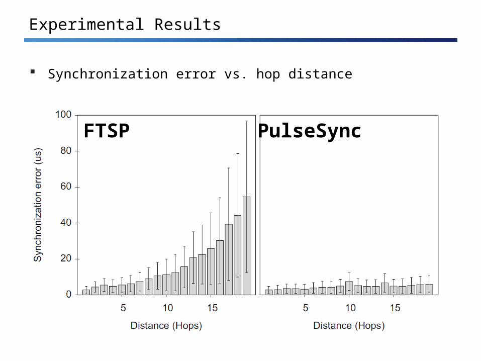
Synchronization error vs. hop distance
Experimental Results
FTSP PulseSync

Problem: So far PulseSync works for list topology only
Instead schedule synchronization beacons without collisions• Time information has to propagate quickly through the network• Avoid loss of synchronization pulses due to collisions
In other words, for the first time in my life as a researcher, theory and practice play ping pong.
Beyond the list?
This is known as wireless broadcasting, a well-studied problem (in theory…!)

Open Problems
• global vs. local skew• worst-case vs. reality (Gaussian?)• accuracy vs. convergence • accuracy vs. energy efficiency • dynamic networks• fault-tolerance (Byzantine clocks)• applications, e.g. coordinating physical objects (example with cars)
• more open problems in SOFSEM paper

…
Everybody‘s expectation, five years ago („solved“)
Lower bound of logD / loglogD[Fan & Lynch, PODC 2004]
All natural algorithms [Locher et al., DISC 2006]
Blocking algorithm
Kappa algorithm[Lenzen et al., FOCS 2008]
Tight lower bound[Lenzen et al., PODC 2009]
Dynamic Networks![Kuhn et al., SPAA 2009]
FTSP PulseSync
Summary

Roger Wattenhofer @ SOFSEM 2010 – 57
Thank You!Questions & Comments?
Thanks to my co-authorsNicolas Burri
Michael KuhnChristoph Lenzen
Thomas LocherPhilipp Sommer
Pascal von Rickenbach

Clock Synchronization