Svensk Kärnbränslehantering ABSwedish Nuclear Fueland Waste Management Co

Box 250, SE-101 24 Stockholm Phone +46 8 459 84 00

R-08-66

CM

Gru

ppen

AB

, Bro

mm

a, 2

009

R-0

8-6

6

Rock mechanics Forsmark Modelling stage 2.3

Complementary analysis and verification of the rock mechanics model

Rune Glamheden, Golder Associates AB

Flavio Lanaro, Johan Karlsson, Ulrika Lindberg

Berg Bygg Konsult AB

John Wrafter, Geo Innova AB

Hossein Hakami, Malin Johansson

Itasca Geomekanik AB

December 2008

Tänd ett lager:

P, R eller TR.

Rock mechanics Forsmark Modelling stage 2.3

Complementary analysis and verification of the rock mechanics model

Rune Glamheden, Golder Associates AB

Flavio Lanaro, Johan Karlsson, Ulrika Lindberg

Berg Bygg Konsult AB

John Wrafter, Geo Innova AB

Hossein Hakami, Malin Johansson

Itasca Geomekanik AB

December 2008

ISSN 1402-3091

SKB Rapport R-08-66

This report concerns a study which was conducted for SKB. The conclusions and viewpoints presented in the report are those of the authors and do not necessarily coincide with those of the client.

A pdf version of this document can be downloaded from www.skb.se.

3

Preface

The report describes the results of the rock mechanics site modelling for the Forsmark area during modelling stage 2.3. The overall aim of the work during modelling stage 2.3 has been to complete the rock mechanics model by including new accessible data of particular value. The purpose has also been to validate the rock mechanics model and reduce the uncertainty of the model a further step.

In addition to the authors, Anders Sundberg has contributed to the rock mechanics modelling work at Forsmark, stage 2.3 by assisting in the stochastic modelling of the uniaxial compressive strength of the intact rock in the rock domains.

The authors acknowledge Rolf Christiansson, Harald Hökmark, Derek Martin, Isabelle Olofsson and Jonny Sjöberg, for examination of the manuscript.

5

Abstract

The Swedish Nuclear Fuel and Waste Management Company (SKB) is undertaking site char­acterization at two different locations, Forsmark and Laxemar/Simpevarp, with the objective of siting a geological repository for spent nuclear fuel. The characterization of a site is an integrated work carried out by several disciplines including geology, rock mechanics, thermal properties, hydrogeology, hydrogeochemistry and surface systems. The present report treats the results from the latest rock mechanics modelling stage 2.3 of the Forsmark area. The report is a complemen­tary report to the main reference report from modelling stage 2.2 /Glamheden et al. 2007a/.

The aim of the work has been to complete the rock mechanics model by including new acces­sible data of great value, furthermore, to validate the model and further reduce the uncertainty of the model.

The results from modelling stage 2.3 confirm the validity of the interpreted model from previous modelling stages. A spatial statistic description of the compressive strength at a rock domain level is also provided through the performed stochastic simulations.

6

Sammanfattning

Svensk Kärnbränslehantering AB genomför platsundersökningar inom två olika områden, Forsmark och Laxemar/Simpevarp, med syftet att lokalisera ett slutförvar för använt kärn­bränsle. De platsbeskrivande modellerna tas fram som ett integrerat arbete och involverar flera olika ämnesområden såsom geologi, bergmekanik, termiska egenskaper, hydrogeologi, hydrokemi och ytnära system. Denna rapport redovisar resultaten från det senaste berg­mekaniska modelleringssteget 2.3 för Forsmarkområdet. Rapporten utgör ett komplement till huvudreferensrapporten från modelleringssteg 2.2 /Glamheden et al. 2007a/.

Syftet med arbetet har varit att slutföra den bergmekaniska modellen genom att inkludera tillgänglig data av stort värde, validera modellen samt reducera osäkerheten i modellen ytterligare en grad.

Resultaten från steg 2.3 bekräftar giltigheten i modellen från tidigare modelleringssteg. En spatial statistisk beskrivning av enaxiella tryckhållfastheten hos det intakta berget på domännivå redovisas också genom den stokastiska modelleringen.

7

Contents

1 Introduction 91.1 Background 91.2 Scope of work and structure of the report 9

2 Mechanical properties of intact rock 112.1 Overview of the primary data 112.2 Strength properties of the intact rock 12

2.2.1 Uniaxial compressive strength 122.2.2 Crack initiation stress 132.2.3 Indirect tensile strength 14

2.3 Deformational properties of the intact rock 152.3.1 Young’s modulus 152.3.2 Poisson’s ratio 16

2.4 Microcrack volume measurements 172.5 Summary and uncertainties 18

3 Stochastic simulation of compressive strength 193.1 Introduction 193.2 Strategy for modelling uniaxial compressive strength 193.3 Geostatistical analyses and stochastic simulations 21

3.3.1 Stochastic simulation of lithologies 213.3.2 Spatial statistical models of compressive strength 213.3.3 Stochastic simulation of UCS in each TRC 23

3.4 Rock domain model of uniaxial compressive strength 253.4.1 Rock domain modelling results 253.4.2 Evaluation of rock domain modelling results 273.4.3 Uncertainties 27

3.5 Summary 28

4 Evaluation of the rock mass mechanical properties using empirical methods 29

4.1 Singö deformation zone 294.2 Forsmark deformation zone 314.3 Comparison with fracture domains and other deformation zones 324.4 Summary 34

5 In situ state of stress 355.1 Borehole breakout 35

5.1.1 Breakout statistics in Forsmark 355.1.2 Breakouts in the complementary boreholes 365.1.3 Compilation of breakout data for all boreholes 40

5.2 Summary 455.3 Visualisation of the in situ stress data 46

5.3.1 Overcoring stress measurements 465.3.2 Hydro­fracturing stress measurements 485.3.3 Summary 48

5.4 Stress variability with depth due to varying modulus 495.4.1 Background 495.4.2 Input data and model set­up 495.4.3 Results 515.4.4 Summary 52

6 Summary 536.1 Intact rock properties 536.2 Rock mass properties 536.3 In situ state of stress 53

7 References 55

Appendix A Simulation of UCS 57

Appendix B Results from empirical modelling 75

Appendix C Data delivery from Sicada 81

9

1 Introduction

1.1 BackgroundThis report presents the results of the rock mechanics modelling work carried out during Forsmark modelling stage 2.3. The work includes activities identified during modelling stage 2.2 as well as new identified complementary activities. This work constitutes the last step in the development of the rock mechanics model.

The aim of the work has been to complete the rock mechanics model by including new acces­sible data of value. The purpose has also been to validate and further reduce the uncertainty in the rock mechanics model. The results will be integrated to the previous version of the rock mechanics model and summarized in the SDM­Site report for Forsmark.

1.2 Scope of work and structure of the reportThe scope of the work includes the following main activities:

• CompilationofadditionallaboratorytestsforfracturedomainFFM06,compilationoftestson samples including sealed fracture network and analysis of additional microcrack volume measurements (Chapter 2).

• Stochasticsimulationsofthevariabilityoftheuniaxialcompressivestrengthinacertainvolume due to subordinate rock types according to the concept developed for the thermal modelling (Chapter 3).

• EmpiricalcharacterizationofboreholesectionsthroughtheForsmarkandSingödeformationzone in borehole KFM011A and KFM012A, respectively (Chapter 4).

• EvaluationofbreakoutsinboreholeKFM08A,08C,09Aand09B(Section5.1).

• VisualisationoftheresultsoftheinsitustressmeasurementsstoredinSicadabyusingRVS(Rock Visualization System), see Section 5.3.

• Numericalmodellingofvariabilityofthestressesinordertoassesstheinfluenceofthevariation of the deformation modulus with depth (Section 5.4).

The report is completed with a number of appendices (A­C). Appendix A addresses the stochas­tic simulations. Appendix B includes results from the empirical modelling. Appendix C, finally, presents the date of delivery of primary data from Sicada used in the rock mechanics modelling.

11

2 Mechanical properties of intact rock

2.1 Overview of the primary dataIn this Section, the mechanical properties from laboratory tests on intact rock are presented and discussed. The presentation concentrates on supplementary tests in the target volume (fracture domain FFM01 and FFM06) that were not included in Forsmark modelling stage 2.2 /Glamheden et al. 2007a/. The section also covers a brief comparison with previous results.

The dominant rock type in fracture domain FFM01 is granite to granodiorite metamorphic, medium­grained (101057), while fracture domain FFM06 comprises mainly albitized aplitic granite (101058). Other mapped rock types in the target volume are tonalite to granodiorite, pegmatite and amphibolite. Detailed information of the rock domain and the fracture domain model is presented in /Glamheden et al. 2007a/.

The laboratory tests on intact rock were performed at SP (the Swedish National Testing and Research Institute). The methodology, standards and performance followed for the testing are described in the following SKB Method Descriptions:

• UniaxialCompression:SKBMD190.001e,ver.4.0(2006-10-31).

• TriaxialCompression:SKBMD190.003e,ver.3.0(2006-10-31).

• IndirectTensileTests:SKBMD190.004e,ver.3.0(2006-10-31).

The number and type of laboratory tests on intact rock carried out in each fracture domain for modelling stage 2.3 are listed in Table 2­1. The performed test program on intact rock includes in total 24 uniaxial compressive tests, 4 triaxial compressive tests and 10 tensile tests. The addi­tional triaxial tests were carried out for determination of the microcrack volume of the intact rock.

The tests were performed mainly on intact, unaltered and non­fractured rock. Five samples in rock domain RFM029 from borehole KFM06A were taken in a deformation zone (ZFMENE0060A) and contain sealed fracture networks. Theses samples were tested for deter­mination of the elastic parameters. Three samples in fracture domain FFM01 and one sample in FFM02 were “affected by the vicinity of a deformation zone” according to the records in Sicada. Furthermore, all samples in FFM06 are affected by albitization.

Table 2‑1. Number of tests for each testing method performed for Forsmark modelling stage 2.3.

Borehole Rock domain Fracture domain

Rock type Uniaxial compressive tests

Triaxial compressive tests

Indirect tensile tests

KFM01A RFM029 FFM01 101057 – 25) –KFM02B RFM029 FFM01 101057 – 25) –KFM01C RFM029 FFM01 1010611) 3 – –KFM01C RFM029 FFM02 101051 4 – –KFM01C RFM029 FFM02 1110581) 1KFM06A RFM029DZ – 1010572) 64) – –KFM08D RFM045 FFM06 1010573) 10 10

1) Samples affected by DZ /Jacobsson 2007e/.

2) Intact rock from ZFMENE0060A containing sealed fracture networks /Jacobsson 2007a/. The rock type classification has been adjusted for these samples in accordance to what is reported in Sicada.

3) The analysed samples are albitized /Jacobsson 2007bc/.

4) One sample failed due to its weak structure and was therefore excluded /Jacobsson 2007a/.

5) Microcrack volume measurements /Jacobsson 2007d/.

12

2.2 Strength properties of the intact rockIn this section, the strength properties of the intact rock for this modelling stage 2.3 are discussed.Theresultsincludeuniaxialcompressivestrength(σc),crackinitiationstress(σci) andindirecttensilestrength(σt).

2.2.1 Uniaxial compressive strengthSamples from fracture domains

The three samples from FFM01 of pegmatite, pegmatitic granite (101061) are all “affected by the vicinity of a deformation zone”. The uniaxial compressive strength of these samples range between 158 MPa and 187 MPa, see Table 2­2. The samples in fracture domain FFM02 include four samples of granite, granodiorite and tonalite (101051) and one sample of granite, fine­ to medium­grained (111058) “affected by a deformation zone”. The uniaxial compressive strength of these samples ranges between 214 MPa and 246 MPa with a mean value of 229 MPa.

The additional test results from fracture domain FFM06 of the altered (albitized) variant of 101057 (granite to granodiorite, metamorphic, medium­grained), range between 338 MPa and 391 MPa with a corresponding mean value of 373 MPa calculated on 10 tests. The additional samples in fracture domain FFM06 confirm the results from modelling stage 2.2 indicating that the compressive strength of rock in FFM6 is considerably higher than in FFM01. The higher strength values of the rock types in domain FFM06 is attributed to the albitization of the rock, which increase the quartz content /Stephens et al. 2007/.

A comparison of the results obtained for pegmatite, pegmatitic granite in Forsmark modelling stage 2.2 /Glamheden et al. 2007a/ and the present modelling stage 2.3 display a reduced mean value of about 6%. A possible reason for the observed strength reduction is that the additional samples are affected by the vicinity of a deformation zone.

Samples from deformation zones

Six samples from borehole KFM06A in domain RFM029 were taken from deformation zone ZFMENE0060A. However, one sample could not be tested due to its weak structure, see /Jacobsson 2007a/. These samples comprise sealed fracture networks. The five samples are composed of the main rock type granite to granodiorite (101057) and their uniaxial compressive strength varies between 191 and 233 MPa, see Table 2­2 and Figure 2­1. The mean value of 220 MPa is only 3% lower than the mean value of the same rock type outside deformation zones in fracture domain FFM01.

Table 2‑2. Uniaxial compressive strength of additional samples evaluated for Forsmark modelling stage 2.3.

Fracture domain Rock Type No. of samples

Minimum (MPa)

Mean (MPa)

Median (MPa)

Maximum (MPa)

Std. dev. (MPa)

FFM01 101061 31) 158 167 158 187 16.8FFM02 101051 4 214 224 227 228 6.9FFM02 111058 11) 246 246 246 246 –FFM06 101057 102) 338 373 382 391 19.8DZ 101057 53) 191 220 223 233 17.1

1) Samples affected by DZ.

2) Albitized samples.

3) Samples from ZFMENE0060A containing sealed fracture networks.

13

2.2.2 Crack initiation stressThe crack initiation stress has been evaluated from the uniaxial compressive tests according to the procedure presented by /Martin et al. 2001/. The value is a measure of the stress required to initiate tensile cracking in laboratory samples.

For pegmatite (101061) samples in fracture domain FFM01, the crack initiation occurs around 90 MPa, see Table 2­3. These samples are “affected by a deformation zone”. For granite, grano­diorite and tonalite (101051) in fracture domain FFM02, the crack initiation occurs at around 122 MPa while for the only available sample of granite, fine­to medium­grained (111058) in FFM02, the crack initiation stress is 170 MPa. For albitized metagranite (101057) in fracture domain FFM06, the crack initiation occurs at around 196 MPa. The additional tests confirm the results from modelling stage 2.2, showing higher crack initiation stress of the albitized rock types from domain FFM06 than for correspondent rock types in FFM01.

The crack initiation stress of the samples containing sealed fracture networks has a mean value of 112 MPa. These results are similar to the results evaluated for the same rock type (101057) in FFM01. The mean value is only about 3% lower for the samples containing sealed fracture networks.

A comparison of the results obtained for pegmatite, pegmatitic granite in Forsmark modelling stage 2.2 /Glamheden et al. 2007a/ and the present modelling stage 2.3 show a slightly reduction of the evaluated mean value of the crack initiation stress. The reason for the difference is pos­sibly that the additional samples are affected by the vicinity of a deformation zone.

Figure 2‑1. Uniaxial compressive strength of samples of metagranite (101057) containing sealed fracture networks from deformation zone ZFMENE0060A.

UCS - samples from ZFMENE0060A

0

1

2

3

<190

190-

200

200-

210

210-

220

220-

230

230-

240

>240

UCS [MPa]

Num

ber o

f sam

ples

14

Table 2‑3. Crack initiation stress of additional samples evaluated for Forsmark modelling stage 2.3.

Fracture domain Rock Type No. of samples

Minimum (MPa)

Mean (MPa)

Median (MPa)

Maximum (MPa)

Std. dev. (MPa)

FFM01 101061 31) 85 90 85 100 8.7FFM02 101051 4 120 122.5 122.5 125 2.9FFM02 111058 11) 170 170 170 170 –FFM06 101057 102) 180 196 190 250 20.1DZ 101057 53) 85 112 120 130 17.5

1) Samples affected by DZ.

2) Albitized samples.

3) Samples from ZFMENE0060A containing sealed fracture networks.

2.2.3 Indirect tensile strengthIn modelling stage 2.2 the tensile strength of fracture domain FFM06 was estimated based on results from adjacent domains /Glamheden et al. 2007a/. To improve the confidence of the tensile strength of the actual domain, indirect tensile tests performed by means of the Brazilian test method, were conducted on 10 samples of albitized metagranite (101057) from FFM06. The results are presented in Figure 2­2.

The evaluated mean value of the tensile strength is 14.8 MPa to be compared with 13.4 MPa for the same rock type in FFM01. The results indicate that albitization has no influence of the tensile strength, since the results are similar in FFM01 and FFM06.

Figure 2‑2. Tensile strength evaluated based on Brazilian tests for samples of albitized metagranite (101057) from fracture domain FFM06.

FFM06

0

1

2

3

4

5

<8

8-10

10-1

2

12-1

4

14-1

6

16-1

8

Tensile strength [MPa]

Num

ber o

f sam

ples

15

2.3 Deformational properties of the intact rock2.3.1 Young’s modulus Young’s modulus is in the present modelling stage 2.3 based on the tangent modulus evaluated at 50% of the uniaxial compressive strength. The results are presented in Table 2­4. The highest values with a mean value of 80 GPa are found for albitized metagranite (101057) from FFM06. The lowest values with a mean value of 71 GPa are for pegmatite, pegmatitic granite (101061) from FFM01, where the samples are “affected by a deformation zone”. The additional samples in fracture domain FFM06 confirm the results from modelling stage 2.2, indicating that the rock types in FFM06 are slightly stiffer than those in FFM01.

The tests performed on samples composed of sealed fracture networks from deformation zone ZFMENE0060A have a mean value of 71 GPa, which is just slightly lower (7%) than the results for samples in FFM01, see Figure 2­3.

The results for pegmatite, pegmatitic granite obtained in Forsmark modelling stage 2.2 and in the present modelling stage 2.3 are similar.

Figure 2‑3. Young’s modulus of samples of metagranite (101057) containing sealed fracture networks from deformation zone ZFMENE0060A.

Table 2‑4. Young’s modulus evaluated from uniaxial compressive tests for additional samples for Forsmark modelling stage 2.3.

Fracture domain Rock Type No. of samples

Minimum (MPa)

Mean (MPa)

Median (MPa)

Maximum (MPa)

Std. dev. (MPa)

FFM01 101061 31) 69 71 70 73 2FFM02 101051 4 73 75 75 76 1FFM02 111058 11) 77 77 77 77 –FFM06 101057 102) 78 80 80 82 1DZ 101057 53) 69 71 71 72 1

1) Samples affected by DZ.2) Albitized samples.3) Samples from ZFMENE0060A containing sealed fracture networks.

Samples from ZFMENE0060A

0

1

2

3

4

<68

68-7

0

70-7

2

72-7

4

74-7

6

76-7

8

78-8

0

80-8

2

82-8

4

84-8

6

>86

Young's modulus [GPa]

Num

ber o

f sam

ples

16

2.3.2 Poisson’s ratio Poisson’s ratio was evaluated from the uniaxial compressive strength tests. The results are presented in Table 2­5. The results in FFM06 (101057) range between 0.26 and 0.31 with a mean value of 0.29. The additional samples in fracture domain FFM06 confirm the results from modelling stage 2.2. The results of the tested samples from the other fracture domains are similar to those from domain FFM06.

The tests performed on samples containing sealed fracture networks from deformation zone ZFMENE0060A, range between 0.24 and 0.27 with a mean value of 0.25, which is similar to the results for samples in FFM01, see Figure 2­4.

The results for pegmatite, pegmatitic granite obtained by Forsmark modelling stage 2.2 and the present modelling stage 2.3 are similar.

Figure 2‑4. Poisson’s ratio of samples of metagranite (101057) containing sealed fracture networks from deformation zone ZFMENE0060A.

Table 2‑5. Poisson’s ratio evaluated from uniaxial compressive tests for additional samples for Forsmark modelling stage 2.3.

Fracture domain Rock Type No. of samples Minimum Mean Median Maximum Std. dev.

FFM01 101061 31) 0.27 0.30 0.30 0.32 0.03FFM02 101051 4 0.28 0.29 0.29 0.29 0.00FFM02 111058 11) 0.29 0.29 0.29 0.29 –FFM06 101057 102) 0.26 0.29 0.28 0.31 0.02DZ 101057 53) 0.24 0.25 0.25 0.27 0.01

1) Samples affected by DZ 2) Albitized samples3) Samples from ZFMENE0060A containing sealed fracture networks.

Samples from ZFMENE0060A

0

1

2

3

<0.1

6

0.16

-0.1

8

0.18

-0.2

0

0.20

-0.2

2

0.22

-0.2

4

0.24

-0.2

6

0.26

-0.2

8

0.28

-0.3

0

0.30

-0.3

2

0.32

-0.3

4

>0.3

4

Poisson's ratio [-]

Num

ber o

f sam

ples

17

2.4 Microcrack volume measurementsCoring of granite at depth may induce microcracking due to stress relaxation and drilling induced effects /Martin and Stimpson 1994/. Significant microcracking affects the mechanical properties of laboratory samples and may provide a systematic bias in the laboratory results of the deformation and strength properties. Microcracking may also influence the hydrogeochemis­try and transport properties of the intact rock.

To estimate the microcrack volume of samples collected in Forsmark, the amount of non­linear volumetric strain recorded in hydrostatic triaxial compression tests was measured /Jacobsson 2007d/. An initial test series of 12 samples on metagranite (101057) from boreholes KFM01A and KFM02B (6 samples from each borehole) was carried out in Forsmark modelling stage 2.2 /Glamheden et al. 2007a/. Modelling stage 2.3 includes two additional samples from each borehole at larger depth. The results from the two series are presented in Figure 2­5 below.

The latest results confirm previous test results, showing a clear linear increase with depth of the microcrack volume for the samples from KFM01A. On the other hand, the samples from KFM02B display no clear variation with depth. Furthermore, the microcrack volume is larger for samples from KFM01A (0.04–0.12%) than from KFM02B (0.02–0.04%).

The uniaxial compressive strength, the indirect tensile strength and Young’s modulus for the dominant rock type all display a slight decrease in the values with depth. The decrease may result from stress­induced microcracking during coring, which are consistent with the above results from the microcrack volume measurements and the P­wave measurements /Glamheden et al. 2007a/. A depth increase in microcrack volume (as the one observed for KFM01A) also implies that the uncertainty on the compressive and tensile strength evaluated at depth is higher. However, it is difficult to draw definitive conclusions from the microcrack volume measure­ments as the depth trend is only visible in one borehole. The results might be a consequence of different sampling and/or testing conditions.

Figure 2‑5. Measured microcrack volume versus elevation for samples of metagranite (101057) from KFM01A and KFM02B.

Microcrack volume strain

0

0.04

0.08

0.12

0.16

0 100 200 300 400 500 600 700 800

Elevation (m)

Mic

rocr

ack

volu

me

(%)

KFM01A

KFM02B

18

2.5 Summary and uncertaintiesIn Table 2­6, a summary of the mechanical properties of the additional samples tested in Forsmark modelling stage 2.3 is presented. An estimation of the uncertainties of the mechanical properties is also proposed based on the 95% confidence interval of the mean value. The uncertainties are given as percentage of the mean value of the properties itself.

The recent results for pegmatite, pegmatic granite (101061) show deformations properties similar to those evaluated in modelling stage 2.2, while the strength properties are slightly reduced. The latest samples all are affected by deformation zones, which may be the reason for the observed lower strength.

The mechanical properties for the rock types in FFM02 are similar to the properties evaluated for the main rock type in fracture domain FFM01 and FFM03.

The additional samples in fracture domain FFM06 confirm the results from modelling stage 2.2. The results for the albitized variants of metagranite (101057) and aplitic granite (101058) within FFM06 clearly demonstrate that the intact rock is stiffer and stronger than that in FFM01. However, the albitization does not seem to have any effect of the tensile strength of tested rock types.

The tests performed on samples composed of sealed fracture networks from deformation zones ZFMENE0060A show results close to what is observed of intact rock in fracture domain FFM01. The sealed fractures seem to have an insignificant influence of the mechanical properties of intact rock except for the crack initiation stress that is slightly lower for the sealed samples.

The latest results from the microcrack volume measurements confirm the previous test results. The samples from KFM01A show a clear linear increase of the microcrack volume strain with depth, while the samples from KFM02B display minor variation with depth.

Table 2‑6. Summary of the deformability and strength properties of the additional samples tested for Forsmark modelling stage 2.3.

Parameter FFM01 FFM02 FFM02 FFM06 DZ101061 Mean/stdev Min – Max Uncertainty

101051 Mean/stdev Min – Max Uncertainty

111058 Mean/stdev Min – Max Uncertainty

101057 Mean/stdev Min – Max Uncertainty

101057 Mean/stdev Min – Max Uncertainty

Number of tests 31) 4 11) 102 53)

Young’s modulus (GPa) 71/2 69–73 ±3%

75/1 73–76 ±1%

77 80/1 78–82 ±1%

71/1 69–72 ±1%

Poisson’s ratio 0.30/0.03 0.27–0.32 ±10%

0.29/0.005 0.28–0.29 ±2%

0.29 0.29/0.02 0.26–0.31 ±4%

0.25/0.01 0.24–0.27 ±4%

Uniaxial compressive strength (MPa)

167/16.8 158–187 ±11%

224/7 214–228 ±3%

246 373/20 338–391 ±3%

220/17 191–233 ±7%

Crack initiation stress (MPa)

90/8.7 85–100 ±11%

123/3 120–125 ±2%

170 196/20 180–250 ±6%

112/18 85–130 ±14%

Number of tests – – – 102 –Indirect tensile strength (MPa)

– – – 14.8/1.3 12.8–16.6 ±5%

–

Note: The uncertainty of the mean is quantified for a 95% confidence interval. Minimum and maximum truncation values are based on observed min’ and max’ for the tested population.1) Samples affected by DZ.2) Albitized samples.3) Samples from ZFMENE0060A containing sealed fracture networks.

19

3 Stochastic simulation of compressive strength

3.1 IntroductionOne issue of importance in the design process of a repository is to estimate the loss of deposi­tion holes due to the risk of spalling, which is one factor which governs the space required. This estimation is partly based on the occurrence and strength of the intact rock of different types. Therefore, stochastic simulation is used to describe the expected spatial distribution of uniaxial compressive strength (UCS) in Forsmark.

The main objectives of the stochastic simulations of UCS are:

1. To provide a spatial statistical description of the UCS at a rock domain level for the Forsmark area. From these results the amount of low strength rock in the target volume may be estimated.

2. To acquire an increased understanding of the spatial correlation structure of UCS of intact rock.

3. To visualize the spatial distribution of UCS.

4. To provide the basis for further study of issues relating to the spatial variability of UCS in and around a repository, using the realisations produced by the simulation.

At Forsmark, two rock domains have been defined within the target volume: domains RFM029 and RFM045 /Stephens et al. 2007/. A compressive strength model is presented for each rock domain.

Although it is known that UCS is a function of scale – it decreases as the volume of rock considered increases /Hoek and Brown 1980/ – the effects of upscaling on the UCS properties of the rock have not been modelled. The simulated UCS values assigned to each 1 m cell relate to a volume corresponding to the sample size (0.1 m) located in the centre of the 1 m cell.

The paucity of data on which to base reliable models is a significant problem associated with the results of this study. However, the study serves to demonstrate the usefulness of stochastic simulations for such investigations, as well as more specifically illustrating the nature of the spatial variability of UCS in Forsmark.

3.2 Strategy for modelling uniaxial compressive strengthThe modelling approach used here is similar to that used for the modelling of thermal properties at Forsmark /Back and Sundberg 2007/ and described in the strategy report /Back and Sundberg 2007/. The approach as applied to the modelling of UCS is summarised below.

The modelling involved stochastic simulation based on both the spatial statistical structure of lithologies and the spatial distribution of UCS.

Stochastic simulations of lithologies were performed for the Forsmark area as part of the thermal modelling, the results of which are reported in /Back et al. 2007, Sundberg et al. 2008/. Each realisation has a simulation volume of 50x50x50 m and each cell represents a 1 m cube. This simulation volume is assumed to be sufficiently large for the objectives of the simulations.

The maximum number of classes that can be handled in the lithological simulations is five /Back and Sundberg 2007/. This required grouping rock types into rock classes (called thermal rock classes (TRCs) in thermal modelling). Each TRC comprises one or more rock types having similar lithological properties. Given that each TRC is generally dominated by a single rock type this simplification has little significance for the overall UCS model at domain level.

20

The basis for the stochastic simulation of UCS is spatial statistical models of UCS for each TRC, describing both probability distributions and spatial correlation. The probability distribution models for different rock types are derived from UCS laboratory measurements. The variability in the UCS measurement data is related to rock type, spatial variation within a rock type, in addition to limitations associated with the testing method.

Spatial correlation models are defined by variograms based primarily on borehole loggings of density, but also UCS data where sufficient data are available. A relationship between density and thermal conductivity for igneous rocks has been observed both between rock types and within rock types at Laxemar /Sundberg et al. 2008/ and Forsmark /Back et al. 2007/, which is not surprising as both properties are closely associated with mineral composition. Thus, for the purposes of thermal modelling, it was reasonably assumed that density and thermal conductivity exhibit similar correlation structures /Back and Sundberg 2007/, which permitted the use of borehole density loggings for the construction of variogram models. It is assumed here that UCS also exhibits a similar correlation structure to density. Support for this assumption is provided by the existence of a correlation between wet density and UCS for some rock types (see Appendix A.1). Thus, density loggings can be employed to construct variogram models for the simulation of UCS. These variograms models are based on the main rock type in each TRC as it is assumed that the spatial correlation structure of the main rock type is representative for the TRC as a whole.

Stochastic simulations of UCS were performed for each rock class (TRC) at two resolutions, 0.1 m and 1 m. The 0.1 m resolution corresponds to the sample support, the size of the UCS samples. The simulated 0.1 m UCS values within each 1 m cube are averaged using the arithmetic mean to produce a new set of values, termed here as “1 m values”. The resulting distribution of 1 m values for each TRC is used as the model for simulation at 1 m resolution. However, no upscaling is implied. The objective of this averaging step is to reduce or eliminate the variability that occurs at distances less than 1 m. This variability is essentially a function of two components: 1) the uncertainties associated with the testing method, and 2) true spatial variability at distances less than 1 m.

For the 1 m simulation step, the simulation volume and resolution are the same as for the lithological simulations. Although the geostatistical simulations have a cell size of 1×1×1 m, UCS is a parameter that relates to intact rock at standard laboratory scale (dm). In other words, each 1 m cell is assigned one UCS value, corresponding to a laboratory­size sample taken in the centre of the cell.

Lithological realisations and the UCS realisations are merged, i.e. each cell in the lithological realisation is filled with the appropriate UCS value from the corresponding position of the UCS realisations. Merging produces a set of realisations of compressive strength for each rock domain that considers both differences between TRCs and variability within TRCs; see Figure 3­1.

Based on these realisations a statistical description of UCS at the domain level is produced. The realisations are also used to provide visualisations of the spatial distribution of UCS. These simulated realisations are used to represent the rock domain statistically, and do not apply to a specific location in the rock mass; in other words the approach is based on unconditional stochastic simulation.

The modelling approach requires a number of assumptions in various steps of the modelling process /Back et al. 2007/. The most important ones are believed to be the following:

• Thegeologicalrealisationsareassumedtoberepresentativeforthemodelledrockdomains.

• ItisassumedthatthespatialstatisticalUCSmodelforaTRC(statisticaldistributionandvariogram) applies to the individual rock types that belong to that TRC.

• UCSisassumedtoexhibitspatialcorrelationstructuresthatmimicthatofdensity.

21

3.3 Geostatistical analyses and stochastic simulations3.3.1 Stochastic simulation of lithologiesThe classification of rock types into rock classes (TRCs) is shown in Table 3­1. The stochastic simulations of lithologies for rock domains RFM029 and RFM045 were performed as part of the thermal modelling, stage 2.2 /Back et al. 2007/ and stage 2.3 /Sundberg et al. 2008/ and are described in detail in the thermal modelling reports. A brief description of the lithological simulations is given in Appendix A.2. Both rock domains were subdivided into more homogenous subdomains in order to capture more of the lithological and structural heterogeneity present. The output from the stochastic simulations of lithologies is used in the modelling of UCS. One hundred realisations of geology for each rock domain were selected for the purpose of modelling UCS. Each realisation has dimensions 50 x 50 x 50 m and a resolution of 1 m. Visualisations of example geology realisations for domain RFM029 and domain RFM045 are presented in Appendix A.8.

3.3.2 Spatial statistical models of compressive strengthSpatial statistical models of UCS (a statistical distribution model and a model describing spatial correlation or dependence) are required for each TRC in order to perform simulations at 0.1 m resolution, which approximates the size of the rock samples used for laboratory measurement. These models, and the realisations at 0.1 m resolution, are used to define models of UCS for simulations at 1 m resolution. The focus below is on the models for 0.1 m resolution.

Statistical distribution models – 0.1 m resolutionTest results UCS for individual rock types are summarised in Appendix A.1. UCS data is plentiful for one rock type only, i.e. the dominant granite to granodiorite (101057). Cluster analysis has been performed on data for rock types for which spatially clustered data may produce a bias in the statistics. A comparison of statistics based on declustered data with those drawn from the original data sets show no significant differences. For this reason, uncensored data sets were used.

Figure 3‑1. Schematic description of the merging of lithological realisations and compressive strength realisations for two TRCs. A maximum of five TRCs can be modelled. The spatial variability of compres-sive strength within each TRC is not illustrated in the figure.

TRC 1

Realisations of compressive strength

TRC 2Realisations of TRCs

Merging

22

A statistical distribution model is fitted to the histogram of UCS for each TRC. This is performed by smoothing the histogram with the smoothing algorithm in the geostatistical software GSLIB /Deutsch and Journel 1998/. Figure 3­2 illustrates the method for TRC 57. This algorithm uses a simulated annealing procedure that honours the sample statistics. Smoothing is required because of small data sets. An alternative would have been to use truncated normal distributions, but such models would not have been more certain than the smoothed histograms. The distribu­tion models for most TRCs are rather uncertain because of the low number of data values.

TRC 51 was divided into three subtypes, A, B and C, because of the wide range of rock composi­tions and UCS values (Appendix A.4). Summary statistics for the distributions used in the simula­tions are given in Table 3­1. The UCS values for TRC 17 and TRC 51C are particularly low.

Figure 3‑2. Left: Histogram and statistics of uniaxial compressive strength (UCS) for TRC 57 based on laboratory measurements of drill core samples. Right: Statistical distribution model of UCS for TRC 57 based on smoothing of the data histogram.

Table 3‑1. Division of rock types into rock classes (TRCs). Dominant rock type in bold. Summary statistics of UCS probability distributions at 0.1 m scale.

TRC Rock name/code Present in rock domain

Mean (MPa) St. dev. (MPa)

57 Granite to granodiorite, 101057 RFM029 222 25Granite, aplitic, 101058

58 Granite, aplitic, 101058 RFM045 352 45Granite to granodiorite, 101057

51 Granodiorite to tonalite, 101051 RFM029, RFM045

(A) 245 13(B) 215 14

Felsic to intermediate volcanic rock, 103076 (C) 148 1761 Pegmatite, pegmatitic granite, 101061 RFM029,

RFM045215 37

Granite, 11105817 Amphibolite, 102017

Diorite, quartz diorite and gabbro, 101033RFM029, RFM045

145 29

23

Spatial correlation models – 0.1 m resolutionVariograms are used to model the spatial correlation structure of UCS within a rock type or TRC. In thermal modelling of the rock domains at Forsmark, it was assumed that any spatial dependence in density also reflects spatial dependence in thermal conductivity /Back et al. 2007/. This is also assumed to be valid for modelling of UCS since density, closely related to mineral composition, displays a correlation with UCS for some rock types (see Appendix A.1). The variogram models for each TRC are thus primarily based on variograms produced from borehole density logging data for the dominant rock type in each TRC, but for some TRCs the nugget of the variograms have been modified slightly after an analysis of the UCS data. Separate variogram models are defined for each of the three subtypes of TRC 51. It is acknowledged that there may be other important factors, such as grain size, controlling the spatial dependence of UCS and which it has not been possible to model. However, it can be stated with some certainty that spatial correlation does exist. Given the paucity of UCS data, the variograms based on density logs represent a reasonable attempt to model this spatial dependence.

Variogram models at sample size resolution, i.e. 0.1 m, for each TRC are presented in Table 3­2.

3.3.3 Stochastic simulation of UCS in each TRCStochastic simulation of UCS was performed for each TRC. The software used to perform the simulations is GSLIB. Each TRC is simulated at two resolutions (0.1 m and 1 m). For the 0.1 m resolution, the statistical distribution and variogram models are defined in Section 3.3.2.

The first simulation step was performed with the goal of obtaining a distribution of typical or mean UCS values for 1 m cubes, with no upscaling implied. The simulated 0.1 m values within each 1 m cube are averaged using the arithmetic mean to produce a new set of values, i.e. “1 m values”. The “1 m values” still represent the UCS at measurement scale (0.1 m), but with the variability occurring at distances less than 1 m removed. The resulting histogram of “1 m values” for each TRC is used as the distribution model for simulations at 1 m resolution (see Appendix A.6). The variogram models for the 1 m resolution (shown in Appendix A.5) are modified from the models used for the 0.1 m resolution according to the principles explained in /Back et al. 2007/.

Table 3‑2. Variogram model parameters used for modelling spatial correlation of UCS for TRCs. Nuggets and sills are standardised to the variance of the empirical data.

TRC Rock type used as basis for variogram

Nugget Basis for nugget Range Model Basis for range and model type (boreholes)

57 101057 0.35 Based on UCS lab data; 25 m Exponen tial KFM05A, KFM07A 58 101058 0.40 Based on density logs,

consideration of nugget for 101057, and investigation of UCS data values

3 m

50 m

(nested model – 2 structures)

Exponen tial

Gaussian

KFM06A, KFM08A

51A 101051 0.50 Based on density logs 5 m Spherical KFM01A, KFM04A51B 101051 0.50 Based on density logs 5 m Spherical KFM06A51C 101051 0.50 Based on density logs 7 m Spherical KFM03A61 101061 0.50 Based on density logs,

consideration of nugget for 101057 and investigation of data values.

15 m Spherical KFM01A, KFM08A

17 102017 0.40 Based on density logs 25 m Spherical Several boreholes

Translation of rock codes to rock names: 101057 = Granite to granodiorite, 101058 = Granite, 101051 Granodiorite to tonalite, 101061 = Pegmatite, 102017 = Amphibolite

24

As regards the 1 m simulations, UCS is still being modelled at sample size (0.1 m); in other words, each 1 m cube is assigned a value corresponding to the UCS of a laboratory size sample taken in the centre of the cell.

For the 1 m simulations, the simulation volume and resolution are the same as for the lithological simulations, i.e. a simulation volume of 50×50×50 m divided into cells (cubes) of size 1×1×1 m. This gives a total number of 125 000 cells in each realisation. One hundred such realisations were produced for each TRC. For each TRC the following plots and diagrams have been produced to illustrate the results and validate the method:1. Histogram of simulated UCS values at 1 m resolution from 100 realisations. (Appendix A.6).

The results for TRC 57 are exemplified in Figure 3­3.2. Variogram reproduction plots for 1 m resolution simulations based on individual realisations

(Appendix A.5).3. Visual representation of simulation results at 1 m resolution. 2D slice through a 3D realisation

(Appendix A.7).

For each TRC, statistics of UCS based on results of the 1 metre simulations are summarised in Table 3­3. Statistics of the measured data are shown for comparison. Table 3­3 also shows the difference between the variance of the 0.1 m values and the variance of the “1 m values”. This variance reduction is a result of the averaging step referred to above.

Figure 3‑3. Histogram of UCS for TRC 57 based on stochastic simulation – 100 realisations.

Table 3‑3. Uniaxial compressive strength statistics for all simulated TRCs.

TRC 1m simulations1) Variance reduction2)

Mean (MPa) St. dev. (MPa) %

17 144 20 42%51A 245 8 61%51B 215 8 60%51C 147 10 58%57 221 19 40%58 353 29 56%61 215 23 54%

1) Simulated values – 1 m resolution. 2) Proportion by which the variance of 0.1 m values is reduced on averaging the 0.1 m values to 1 m values.

25

Analysis of results

• Simulationshavesucceededinreproducingratherwellthestatisticaldistributionmodelsused as input in the simulations. In particular, there is very close correspondence between the means of the realisations and the underlying models. However, the variances of the combined realisations at 1 m resolution are slightly lower than the variances of the model; see Appendix A.4.

• Simulationshavesucceededinreproducingratherwellthespatialdependencemodelsusedasinput in the simulations. The results of variogram reproduction are presented in Appendix A.5. Plots compare the variograms calculated from the realisations with the modelvariograms on which simulations at 1 m resolution were based.

• Themeansofsimulated0.1mresolutionvalueswithin1mcubesproduceadistributionwitha marked reduction in variance, from 40 to 60%, compared to the distribution for the 0.1 m values. This reduction in variance corresponds to the variability that occurs at distances less than 1 m, which is a combination of variability due to uncertainties in the testing method but also some of the true spatial variability at sample scale, i.e. at distances less than 1 m. The remaining variability is primarily a function of the spatial variability in UCS within a rock type at distances larger than 1 m.

3.4 Rock domain model of uniaxial compressive strength3.4.1 Rock domain modelling resultsThe results of compressive strength simulations at rock domain level for domains RFM029 and RFM045 are presented in this section.

The realisations of stochastic simulations of lithologies and the realisations from UCS simula­tions, both with a resolution of 1 m, are merged with each other as described in Section 3.2. Results of stochastic simulations of lithologies are presented in /Back et al. 2007/ for domain RFM029 and /Sundberg et al. 2008/ for domain RFM045.

Examples of 2D­visualisations of UCS at domain level and the corresponding geological realisations are presented in Figure 3­4 (more examples in Appendix A.8).

Histograms of UCS for domain RFM029 and domain RFM045 each based on 100 realisations are shown in Figure 3­5 and Figure 3­6. Summary statistics of the realisations are presented in Table 3­4.

Table 3‑4. Summary statistics of results of simulation of uniaxial compressive strength (1 m resolution) for domains RFM029 and RFM045.

RFM029 RFM045Statistical parameter (MPa) (MPa)

Mean 217 310Standard deviation 26 762.5-percentile 143 1365-percentile 168 150

26

Figure 3‑4. Example 2D visualisations from 3D realisations (resolution = 1 m, distance in metres) illustrating the distribution of compressive strength in MPa (left) and corresponding realisation of lithology or TRCs (right) in domain RFM029 and RFM045.

Figure 3‑5. Histogram of compressive strength of rock domain RFM029 simulated at 1 m resolution.

27

3.4.2 Evaluation of rock domain modelling resultsThe lower tail of the UCS distribution is of importance for the design of a repository. Therefore, the 2.5 percentile and 5 percentile of the UCS distribution were estimated for each domain; see Table 3­4. The results indicate that rock domain RFM045 has a more pronounced lower tail than domain RFM029. The estimated probability for values lower than 150 MPa is estimated to be 3% in rock domain RFM029 and to be 5% in domain RFM045. In both domains, the lower tail is a result of low strength rocks, mainly amphibolite (TRC 17) and tonalitic varieties of granodiorite to tonalite (TRC 51C).

There are reasons to believe that the lower tail of the distribution for domain RFM029 is too large due to discretisation error. The discretisation of the simulation volume into 1 m cells results in a significant error when a rock occurs as bodies smaller than 1 m (such occurrences in boreholes are either assigned a full cubic meter or omitted altogether). Amphibolite (TRC 17) commonly occurs as small dyke­like bodies less than 1 m thick /Stephens et al. 2007/, and is also the rock type with the lowest observed UCS values. Since amphibolite in domain RFM045 is present as larger rock bodies than in domain RFM029, the discretisation error is expected to be lower for domain RFM045 than for domain RFM029 /Sundberg et al. 2008/.

The domain histograms of UCS provide a measure of the total spatial variability minus the variability at distances less than 1 m for the sample scale present within a rock domain. This spatial variability can be appreciated to some extent from an inspection of the visualisations.

3.4.3 UncertaintiesThe following uncertainties have been identified.1. For all TRCs with the exception of TRC 57, the statistical distribution models of UCS are

poorly constrained, because of an insufficient number of data values. This is particularly so for the tails of the distribution models. Thus the lower percentile estimates of the UCS distributions at domain level are rather uncertain.

2. Models of spatial correlation of UCS, expressed in the form of density variograms, are based on the assumption that UCS exhibits a spatial correlation structure similar to that of density. Other characteristics (e.g. grain type, grain size and structural fabric) that may influence the UCS of rock have not been considered. These may be particularly important for pegmatite (TRC 61), which displays a wide range in UCS values with no obvious correlation with density. Variation in the proportions of quartz, K­feldspar and plagioclase, the dominant minerals in pegmatites, has only a small effect on density. Moreover, pegmatite typically displays a wide range in grain size.

Figure 3‑6. Histogram of compressive strength of rock domain RFM045 simulated at 1 m resolution.

28

3. Uncertainties associated with the grouping of rock types into rock classes (TRC) are considered to be small given that each TRC is dominated by a single rock type.

4. The simulation resolution chosen for lithological simulations, i.e. 1 m, may produce too conservative estimates of the lower percentiles for rock domain RFM029 due to discretisation errors. The magnitude of this uncertainty is not quantified.

5. The simulation technique is a source of uncertainty. In particular, there is reason to believe that the variance in the output from the 1 m simulations for each TRC has been underestimated by up to 10%. However, since the between­rock variability is larger than the within­rock variability, the underestimation of variance at rock domain level is believed to be small. To reduce the uncertainty, it would be necessary to increase the simulation volume and make adjustments to the simulation parameters.

3.5 SummaryThe spatial variability of uniaxial compressive strength within and between different rock types has been modelled for two rock domains within the target volume at Forsmark. The output from modelling is sets of realisations of compressive strength generated by stochastic simulation. These realisations can be used for future modelling efforts.

The results of the stochastic simulations confirm the validity of the previous SDM site descrip­tive models, and support and strengthen the previous understanding of the spatial variability of UCS within rock type and rock domains. Despite the recognised uncertainties, the stochastic simulations have shown that spatial variability within individual rock types makes up a signifi­cant portion of the total variability observed in the measurement data.

According to the results, rock domain RFM029 has a lower mean compressive strength than domain RFM045. However, the latter rock domain displays greater variability and has a larger proportion of rock with low compressive strength (< 150 MPa).

Stochastic simulation is a valuable tool for modelling properties in a rock mass, and has been successfully used in modelling of thermal properties at both Forsmark /Back et al. 2007/ and Laxemar /Sundberg et al. 2008/. One of the problems encountered in the simulations of UCS presented here is that the spatial statistical models for each rock class (TRC) are based on small amounts of data and uncertain assumptions regarding the nature of spatial correlation. Confidence in the results of the stochastic simulations would increase if more reliable models could be established.

29

4 Evaluation of the rock mass mechanical properties using empirical methods

The empirical characterization of the rock mass was performed based on the data from borehole KFM11A and KFM12A for borehole sections of 5 meters according to the Q and RMR classifi­cation systems and the methodology developed by /Andersson et al. 2002, Röshoff et al. 2002/. The boreholes were drilled through the Singö Deformation Zone (ZFMWNW0001) for a length of about 580 m (KFM11A) and through the Forsmark Deformation zone (ZFMWNW0024) for a length of about 210 m (KFM12A), respectively.

The values of Q and RMR were obtained based on geological information on the open and partly open fractures logged along the boreholes for the purpose of characterization of the rock mass. The effect of water pressure and in situ stresses has to be added to obtain the rock mass quality applicable to design of underground excavations.

The results of the Q­ and RMR­rock mass characterizations in the deformation zones, as well as estimated rock mechanics properties based on empirical relations between RMR/GSI, are summarized in Section 4.1 and 4.2. Variations of Q and RMR and estimated rock mechanics properties along the boreholes are provided in Appendix B.

In relation to the deformation zone as identified by the single­hole interpretation, short additional sections of borehole KFM11A and KFM12A were characterized in the surrounding rock mass for the purpose of comparison. The empirical characterizations accordingly include borehole length 220–845 m in KFM11A and borehole length 145–415 m in KFM12A.

4.1 Singö deformation zoneThe results of the rock mass characterization are shown in Table 4­1 for the deformation zone and the surrounding rock units.

The empirical characterization shows a large variation of the rock mass quality within the Singö deformation zone. The mean value of Q varies between 4.7 and 203 along the characterized borehole sections, which ascribe the rock to classes between “fair and excellent good” qualities. Corresponding results for RMR assign the rock between the class of “very good rock” and “good rock”, however only two points from the threshold towards “fair rock” (which is 60).

On average, the rock in the Singö Deformation Zone along borehole KFM11A has a Q value of 34.5 (mode value of 27.4) and a RMR of 73, which happen to be in “good rock” classes accord­ing to both classification systems. Explicitly considering the effect of water pressure and in situ stresses might lead to more conservative determinations.

It can be observed that the rock mass quality according to Q and RMR in the short analysed sections of borehole outside the deformation zone assigns the rock mass to the class of “good” or “very good” rock, thus showing a clear improvement of the material properties outside the deformation zone.

30

Table 4‑1. Estimated mechanical properties of the rock mass of Singö deformation zone (DZ1) and surrounding rock based on the empirical rock mass characterization of borehole KFM11A.

Division of the deformation zone1)

Q2) [–]

RMR [–]

Fracture frequency3)

[Fract./m]

Deformation modulus [GPa]

Poisson’s ratio [–]

UCSm(H‑B) [MPa]

Friction angle4) [deg]

Cohesion4) [MPa]

Mean[Mode] Min–max5)

Mean/std. dev. Min–max5)

Mean/std. dev. Min–max

Mean/std. dev. Min–max

Mean/std. dev. Min–max

Mean/std. dev Min–max

Mean/std. dev. Min–max

Mean/std. dev. Min–max

KFM11A – RU2 220 – 245

47.5[18.8] 12.9–103.2

77.9/3.8 73.4–82.0

1.1/0.5 0.6–1.8

50.8/11.0 38.4–63.0

0.24/0.05 0.18–0.29

28.2/5.9 21.6–34.8

43.0/1.1 41.8–44.2

17.3/1.0 16.2–18.4

KFM11A – DZ1 RU3a 245 –355

47.4[39.8] 15.5–203.4

74.0/3.6 66.2–83.7

3.2/1.5 1.0–7.0

40.7/9.1 25.5–69.7

0.18/0.05 0.12–0.32

25.1/7.0 14.7–43.4

42.6/1.7 39.7–47.2

16.9/1.3 14.8–20.5

KFM11A – DZ1 RU4 355 – 375

31.2[32.7] 12.6–46.5

72.5/2.5 69.8–75.0

4.4/1.6 3.2–6.8

36.8/5.3 31.2–42.2

0.15/0.02 0.13–0.18

26.2/4.9 21.8–32.1

43.7/1.1 42.5–45.1

17.5/0.9 16.6–18.6

KFM11A – DZ1 RU3b 375 – 410

34.3[29.6] 20.2–63.3

71.8/3.9 67.1–77.0

4.5/2.4 1.0–7.8

35.9/7.9 26.7–47.2

0.15/0.03 0.12–0.19

25.7/9.8 15.2–44.8

41.8/1.5 39.9–44.2

16.6/1.4 14.9–19.3

KFM11A – DZ1 RU5 410 – 585

29.9[22.1] 4.9–113.3

70.7/3.7 63.0–78.5

5.3/2.1 1.6–11.4

33.7/7.3 21.2–51.5

0.15/0.03 0.10–0.23

21.9/7.0 12.2–47.7

41.6/1.6 38.7–45.6

16.2/1.2 14.2–19.3

KFM11A – DZ1 RU6a 585 – 660

17.1[16.7] 4.7–32.2

72.7/3.3 65.2–79.9

5.4/2.2 2.2–9.6

37.6/7.3 24.1–55.8

0.13/0.03 0.08–0.19

48.8/13.0 24.6–76.7

48.1/1.9 43.0–50.7

21.5/2.0 17.0–25.2

KFM11A – DZ1 RU7a 660 – 700

46.8[36.6] 19.5–133.5

72.5/3.1 67.6–78.2

3.6/1.3 1.8–5.8

37.0/6.9 27.6–50.6

0.16/0.02 0.13–0.19

23.3/7.1 15.7–38.5

41.1/0.8 40.1–42.5

16.1/0.7 15.0–17.2

KFM11A – DZ1 RU8 700 – 725

40.2[35.6] 26.7–66.3

78.0/4.6 72.7–85.4

3.2/1.1 2.0/4.0

51.7/15.0 36.9–76.9

0.16/0.04 0.13–0.23

51.5/16.6 31.5–77.6

47.6/1.7 45.1–49.8

21.5/2.3 18.6–24.9

KFM11A – DZ1 RU7b 725 – 785

42.0[37.1] 26.4–85.5

73.2/5.2 67.6–86.6

4.3/1.7 2.0–6.8

39.6/13.8 27.5–78.5

0.16/0.05 0.12–0.30

31.2/12.7 15.6–63.4

43.8/2.1 40.0–48.1

18.0/2.0 15.0–22.8

KFM11A – DZ1 RU6b 785 – 825

26.6[27.0] 14.8–40.6

74.2/2.5 70.2–78.5

4.9/2.1 2.8–8.4

40.6/6.0 32.0–51.7

0.14/0.03 0.11–0.20

49.1/8.0 36.1–63.3

47.2/2.4 43.3–49.8

21.1/1.7 18.3–23.6

KFM11A – RU7c 825 – 845

144[131.5] 88.0–225.0

77.5/2.8 74.3–81.1

1.6/1.0 0.8–3.0

49.2/8.0 40.6–59.8

0.16/0.02 0.13–0.19

46.9/7.7 38.8–57.3

46.4/0.9 45.5–47.6

20.5/1.1 19.3–22.0

1) Length along the borehole (m). 2) For Q, the mode value is reported in brackets beside the mean. 3) Containing open and partly open fractures. 4) For confinement stress between 10 and 30 MPa. 5) Min – Max is based on mean values for borehole sections of 5 m.

31

The fracture frequency varies from 1 to 11 fractures per metres in the zone. Extensive crushed rock according to the BOREMAP definition was encountered in 24 borehole sections of the analysed part of the borehole (220–845 m). The largest crushed rock section extends for a length of 2.1 m and several sections occur within short distance. The reduced rock mass quality due to such conditions is considered in the calculation of Q and RMR.

Table 4­1 also shows the deformability and strength properties of the rock units inside and in the vicinity of the deformation zone. The deformation modulus, Poisson’s ratio, uniaxial compres­sive strength, friction angle and cohesion of the rock mass are obtained by means of the relation between these parameters and RMR/GSI. The values of the Poisson’s ration are only indicative since they are assumed to be proportional to the Poisson’s ratio of the intact rock and to the ratio between the deformation modulus of the rock mass and that of the intact rock.

4.2 Forsmark deformation zoneTable 4­2 contains the results of the characterization by means of Q and RMR of the Forsmark deformation zone (DZ2) based on data obtained from borehole KFM12A. The fracture fre­quency and the derived deformability and strength properties are also summarized in this table.

For the Forsmark zone, the mean Q­ and RMR­values are not necessarily much lower than for the surrounding rock. For example, unit RU3a above the zone exhibits a RMR­value of 69 that is lower than the mean for the whole zone (73), while RU9a below the zone presents a Q­mode value of 28 that is also lower than the mode value for the whole zone (34.4). The Forsmark zone, however, shows minimum values of the rock quality well below the surrounding rock mass, with a mean value of Q 9.7 in one section (“fair rock”) and corresponding values for RMR of 65 in another section (“good rock” class). Locally, sections of “good” (upper range for RMR) and “very good” rock (for Q) occur as indicated by the maximum values. Table 4­2 also shows the deformability and strength properties of the rock mass, with some reservations about the reported values of the Poisson’s ratio (see Section 4.1).

The fracture frequency varies from 2 to 12 fractures per meter in the zone. No crushed rock sections of significant extension (longer than 1 m) were encountered in the analysed part of the borehole (145–415 m). The maximum observed extension of crushed rock was 36 cm.

32

Table 4‑2. Estimated mechanical properties of the rock mass of Forsmark deformation zone (DZ2) and surrounding rock based on the empirical rock mass characterization of borehole KFM12A.

Division of the deformation zone1)

Q2 [–]

RMR [–]

Fracture frequency3)

[Fract./m]

Deformation modulus [GPa]

Poisson’s ratio [–]

UCSm(H‑B) [MPa]

Friction angle4) [deg]

Cohesion4) [MPa]

Mean[Mode] Min–max5)

Mean/std. dev. Min–max5)

Mean/std. dev. Min–max

Mean/std. dev. Min–max

Mean/std. dev. Min–max

Mean/std. dev. Min–max

Mean/std. dev. Min–max

Mean/std. dev. Min–max

KFM12A – RU2 145–170

38.1[36.9] 31.5–50.3

76.7/4.6 72.1–82.6

4.3/2.3 1.6–6.8

47.8/12.7 35.7–65.4

0.15/0.03 0.11–0.20

49.3/11.7 37.2–65.4

47.5/1.2 46.2–48.8

21.2/1.6 19.6–23.3

KFM12A – RU3a 170–190

33.4[33.5] 19.9–46.6

69.2/0.6 68.3–69.5

9.1/2.0 6.8–11.0

30.2/1.0 28.7–30.8

0.11/0.02 0.09–0.13

26.1/6.8 19.5–32.0

44.0/2.0 42.1–45.7

17.6/1.5 16.2–18.9

KFM12A – DZ2 RU3b 190–265

34.3[35.4] 11.5–45.4

71.4/3.2 65.1–76.5

7.5/2.4 4.0–12.2

34.8/6.1 23.9–46.0

0.11/0.02 0.07–0.14

35.6/6.0 25.1–46–2

46.0/0.8 44.4–47.1

19.3/0.9 17.8–20.7

KFM12A – DZ2 RU5 265–285

40.4[44.8] 16.0–56.0

73.3/2.2 70.6–75.9

7.1/1.3 5.2–8.0

38.4/4.8 32.8–44.4

0.15/0.02 0.13–0.17

36.3/4.4 30.8–41.3

42.4/1.2 41.1–44.1

17.7/0.9 16.7–18.5

KFM12A – DZ2 RU6 285–315

28.1[28.7] 12.0–40.0

73.8/2.5 71.8–78.5

5.1/1.2 3.4–6.6

39.7/6.2 35.1–51.5

0.12/0.02 0.11–0.17

38.1/4.1 33.9–44.9

45.1/1.8 42.5–46.9

19.1/1.0 17.6–20.2

KFM12A – DZ2 RU7 315–340

31.6[28.4] 9.7–59.4

75.9/2.6 71.9–77.7

4.7/2.2 2.4–7.4

44.8/6.2 35.2–49.4

0.14/0.01 0.12–0.15

45.0/8.4 31.0–50.6

47.2/1.2 45.1–47.9

20.7/1.3 18.5–21.5

KFM12A – DZ2 RU4b 340–350

16.4[16.4] 12.4–20.4

74.4/0.9 73.7–75.0

3.2/0.6 2.8–3.6

40.7/2.1 39.2–42.2

0.16/0.02 0.15–0.17

39.2/0.7 38.7–39.7

45.2/0.8 44.7–45.8

19.2/0.4 18.9–19.5

KFM12A – DZ2 RU8a 350–400

49.9[42.5] 20.9–173.2

74.9/1.9 72.8–78.7

3.2/1.2 2.2–5.4

42.2/4.9 37.1–52.3

0.13/0.02 0.11–0.18

42.9/5.2 36.1–53.3

46.9/0.7 45.8–48.0

20.3/0.7 19.4–21.8

KFM12A – RU9a 400–415

25.9[27.7] 18.0–32.1

80.2/4.2 75.3–83.2

1.4/0.2 1.2–1.6

57.9/13.1 42.9–67.4

0.24/0.07 0.17–0.31

39.7/7.7 32.9–48.0

45.5/1.1 44.8–46.8

19.4/1.1 18.6–20.7

1) Length along the borehole (m). 2) For Q, the mode value is reported in brackets beside the mean. 3) Containing open and partly open fractures. 4) For confinement stress between 10 and 30 MPa. 5) Min–Max is based on mean values for borehole sections of 5 m.

4.3 Comparison with fracture domains and other deformation zones

The characterization results for Forsmark modelling stage 2.2 provided rock mass quality for the rock mass and deformation zones. Most of such zones were located in the target volume, however, are not ascribed to the group of “regional” deformation zones which is the case for the Singö and Forsmark deformation zone. For the sake of comparison, Table 4­3 was compiled considering the range, mean and mode value of the rock mass quality according to the Q­ and RMR­systems applied for the purpose of characterization. (The effect of water pressure and in situ stresses has to be added to obtain the rock mass quality applicable to design of underground excavations.)

33

It can be immediately observed that the rock mass in the fracture domains is ascribed to the class of “very good” or “extremely good” rock quality respectively according to Q and RMR­system. The fracture domains strictly do not include any deformation zone significant from a rock mechanics point of view, as shown by the minimum rock quality values that are all in the classes of “fair” or “good” rock.

The deformation zones inside the target volume exhibit slightly lower rock mass quality, but, on average, still belong to the class of “very good” rock. These zones, however, show locally some of the lowest rock mass quality of the whole site and with the same magnitude as for the Singö and Forsmark deformation zones. Compared to these regional deformation zones, the major, minor and possible zones present a much wider variation of the rock mass quality, that indicates that their quality can be locally low, but on average very good.

In general, either the major, minor or possible deformation zones exhibit as low rock mass qual­ity as the Singö and Forsmark deformation zones. While the mean quality of the regional zones ranges in the middle of the “good rock” class for both the classification systems, for the other zones, the rock mass quality reach the class of “very good rock”. The regional zones also show the lowest maximum values of all zones.

Table 4­4 contains the mechanical properties estimated for the whole borehole sections inter­cepting the Singö and Forsmark deformation zones and obtained from the RMR­values through the relations between GSI and the deformability and strength parameters of the rock mass. These values can be used to model the two regional deformation zones as equivalent continuum elastic media. The same comment on the Poisson’s ratio as in Section 4.1 applies.

Table 4‑3. Comparison of Q and RMR values for fracture domains FFM01 and FFM06, for deformation zones in the target volume and for Singö and Forsmark deformation zone. The reported values correspond to borehole sections of 5 m.

Q‑value RMR‑valueFracture domain Length (m) Min Mean [Mode] Max Min Mean [Mode] Max

Fracture domainFFM01 2,565 5.5 477 [150] 2,133 73.7 89.1 [89.6] 98.5FFM06 525 20.1 287 [150] 800 73.9 86.7 [87.8] 94.0Deformation zonesMajor DZ 750 1.8 66.2 [28.6] 1,067 64.2 81.2 [80.1] 94.0Minor DZ 350 3.9 54.7 [33.0] 400 70.0 81.6 [81.0] 93.6Possible DZ 255 10.3 99.0 [59.5] 1,067 74.8 81.5 [80.6] 91.1Singö DZ 580 4.7 34.5 [27.4] 203 63.0 72.7 [72.8] 86.6Forsmark DZ 210 9.7 36.2 [34.4] 173 65.1 73.1 [73.5] 78.7

Note: Min–Max are based on mean values for borehole sections of 5 m.

Table 4‑4. Summary of the estimated mechanical properties of the Singö and Forsmark deformation zone.

Properties of the deformation zones

Q1) [–]

RMR [–]

Deformation modulus [GPa]

Poisson’s ratio [–]

Friction angle2)

[deg]Cohesion2) [MPa]

Mean[Mode] Min–max

Mean/std. dev. Min–max

Mean/std. dev. Min–max

Mean/std. dev. Min–max

Mean/std. dev. Min–max

Mean/std. dev. Min–max

Singö DZ 34.5[27.4] 4.7–203.4

72.7/4.0 63.0–86.6

37.9/9.4 21.2–78.5

0.15/0.04 0.08–0.32

43.5/3.0 38.7–50.7

17.8/2.5 14.2–25.2

Forsmark DZ 36.2[34.4] 9.7–173.2

73.1/3.1 65.1–78.7

38.3/6.7 23.9–52.3

0.12/0.03 0.07–0.18

45.7/1.7 41.1–48.0

19.4/1.3 16.7–21.8

1) The mode value of Q is reported in brackets beside the mean. 2) For confinement stress between 10 and 30 MPa.

34

4.4 SummaryThe mechanical properties estimated for the Singö deformation zone based on the empirical modelling presented here indicate a stiffer and stronger rock mass than the estimations based on back­calculation from displacements measurements in the SFR­tunnel passage of Singö deformation presented by /Glamheden et al. 2007b/, see Table 4­5. The results from the empiri­cal characterization are nearest comparable with the back­calculated properties for the altered sector of Singö deformation zone.

There are several reasons that may explain the difference between the results of the two approaches for the estimation of the rock mass mechanical properties. For instance, there are differences that may influence the results in the size of the rock volume analysed and the depth of the tunnel and borehole observations. Furthermore, the size of the zone as defined by the single hole interpretation is not exactly the same as defined by /Glamheden et al. 2007b/.

Another conceivable explanation for the difference in the estimated rock mass properties is simply that the deformation zone is heterogeneous. Such hypothesis is supported by the obser­vation in the discharge tunnels for nuclear power stations in Forsmark and the access tunnels to SFR that goes through the deformation zone/Glamheden et al. 2007b/.

The fact that the empirical approach seem to overestimate the rock mass quality of the deforma­tions zones can also be due to the circumstance that the reduction factors that take into account the water pressure, the in situ rock stresses and the orientation of the tunnel with respect to that of the dominant fracture sets are not considered for the characterization, which should provide the material properties irrespective to the boundary conditions. If these reduction factors are applied, lower strength and larger deformability would be obtained.

The mechanical properties of the deformations zones for use in the regional stress modelling has been estimated based on the theoretical approach /Glamheden et al. 2007a/, with properties for Singö deformation zones collected from /Glamheden et al. 2007b/. This implies that the deformation and strength assumed for the Singö and Forsmark deformation zone in the stress modelling are lower than the properties presented here based on the empirical approach.

Table 4‑5. Estimated rock mass mechanical properties of Singö deformation zone based on back‑calculation from displacements measurements in the SFR‑tunnel passage /Glamheden et al. 2007b/.

Zone sector Deformation modulus [GPa] Poisson’s ratio [–] Friction angle [deg] Cohesion [MPa]

Host rock 45 0.36 65 4.0Altered sector 32 0.43 51 4.0Tabular sector 16 0.43 51 2.0Fractured sector 8 0.43 51 2.0Zone core 3 0.43 37 2.0

35

5 In situ state of stress

The purpose of the rock stress modelling in stage 2.3 is to provide further confidence in the esti­mation of the state of stress in the Forsmark area. The stress modelling in stage 2.3 has include evaluation of breakouts in some additional boreholes, visualisation of the in situ stress data in Sicada using RVS and numerical modelling of the stress variability with depth depending of varying modulus.

5.1 Borehole breakoutThis section presents a complementary study of borehole breakouts in Forsmark conducted on borehole KFM08A (April 2005 and March 2007), KFM08C, KFM09A and KFM09B to validate previously determination by /Martin 2007/ of the trend of the maximum horizontal stress in the Forsmark area.

5.1.1 Breakout statistics in ForsmarkTable 5­1 and Table 5­2 summarize the results from the interpretation of the televiewer logging including both the previous and the presents study. Note that the survey length varies between boreholes. The terminology used for classification of the breakout (BB – Borehole breakout, MF – Micro­fallout, WO – Washout, KS – Keyseat is defined in /Ringgaard 2007a/. The term “classical” applies to breakouts with obvious diametrically opposite deep fallouts /Ringgaard 2007a/.

Table 5‑1. Summary of the breakout length by breakout class. Data is taken from Sicada, survey length for boreholes KFM01A–KFM07C is taken from /Martin 2007/ and /Ringgaard 2007b/ and KFM08A–KFM09B is taken from Sicada.

Borehole name Survey length [m]

Length [m] Total length [m]Borehole

breakouts (BB)Micro‑fallout (MF)

Washout (WO)

Keyseat (KS)

KFM01A 1,000 18.4 278.1 4.8 0.8 302.1KFM01B 480 23.5 118.5 0.8 70.7 213.5KFM02A 979 55.2 91.7 4.4 2.5 153.8KFM03A 989 21.2 81.6 1.0 0.2 104.0KFM03B 83 0.2 30.7 1.2 0.0 32.1KFM04A 984 30.8 70.6 1.0 2.4 104.8KFM05A 990 23.0 47.8 7.8 1.0 79.6KFM06A 933 6.7 8.2 1.0 0.8 16.7KFM07C 512 26.5 178.0 2.9 0.3 207.7KFM08A1) 886 2.2 3.5 3.0 0.1 8.8KFM08A2) 886 2.2 104.9 3.0 0.3 110.4KFM08C 840 9.2 23.7 – 0.1 33.0KFM09A 781 16.4 55.0 3.8 – 75.2KFM09B 598 4.2 49.4 3.2 – 56.8Total [m] 10,055 237.5 1,138.2 34.9 79.1 1,489.7% of surveyed length 2.4 11.3 0.35 0.79 14.8

1) April 2005 – Low resolution in the Televiewer logging /Ringgaard 2007b/ (Not included in the calculated mean values). 2) March 2007 – High resolution in the Televiewer logging /Ringgaard 2007a/.

36

A comparison between the results obtained in the present and the previous study reveals no remarkable differences in the proportions of surveyed length and evaluated mean azimuth due to the enlarged number of boreholes. However, when comparing the results from the two dif­ferent logging occasions in the same borehole (KFM08A), the amount of micro­fallout (MF) is significantly higher the second time. In this case, however, the results are not fully comparable since the applied logging resolution is not the same /Ringgaard 2007a/. This also means that the accuracy of the micro­fallout observations is much higher in the second campaign (March 2007), which is a natural consequence of the higher resolution (the difference for detecting BB is less significant).

5.1.2 Breakouts in the complementary boreholesFigure 5­1 and Figure 5­2 shows the location and azimuth for the different classes of borehole geometry anomalies for the complementary boreholes, KFM08A (at two occasions April 2005 and March 2007) respectively KFM08C, KFM09A and KFM09B.

For the boreholes KFM08A (March 2007), KFM08C, KFM09A and KFM09B rose diagrams that shows the orientation of the “classical” breakouts (BB), not associated with structures, are given in Figure 5­3. Micro­fallouts (MF) that are not associated with structures are shown in Figure 5­4 and keyseats (KS) not associated with structures in Figure 5­5. They all show a general NE­ENE direction. For mean azimuth values, see Table 5­2.

Table 5‑2. Summary of the breakout azimuth by breakout class. Data is taken from Sicada, Survey length for boreholes KFM01A–KFM07C is taken from /Martin 2007/ and /Ringgaard 2007b/ and KFM08A–KFM09B is taken from Sicada.

Borehole name Borehole Inclination3) [°]

Survey length [m]

Mean azimuth 4) [°]Borehole breakouts (BB)

Micro‑fallout (MF)

Washout (WO)

Key seat (KS)

KFM01A –84.72 1,000 68.9 45.0 57.0 50.3KFM01B –79.03 480 53.3 45.8 64.0 50.3KFM02A –85.37 979 78.0 80.7 115.0 102.0KFM03A –85.74 989 47.2 65.9 61.0 32.0KFM03B –85.29 83 77.0 22.0 – –KFM04A –60.07 984 59.3 56.0 41.0 98.0KFM05A –59.80 990 78.5 93.3 – 85.0KFM06A –60.24 933 56.0 34.7 56.0 100.0KFM07C –85.32 512 59.0 56.0 44.0 –KFM08A1) –60.84 886 77.0 47.5 124.0 32.0KFM08A2) –60.84 886 72.0 60.2 – 42.0KFM08C –60.47 840 74.0 100.8 – 34.0KFM09A –59.45 781 49.7 60.8 70.0 –KFM09B –55.07 598 47.0 62.7 58.0 –Mean azimuth [°] 63.1 63.4 67.9 67.3

1) April 2005 – Low resolution in the Televiewer logging /Ringgaard 2007b/ (Not included in the calculated mean values). 2) March 2007 – High resolution in the Televiewer logging /Ringgaard 2007a/. 3) The accuracy in the measurements is less in boreholes deviating more than 10 deg from vertical /Ringgaard 2007a/. 4) The mean values are calculated as point values (not weighted with respect to breakout length).

37

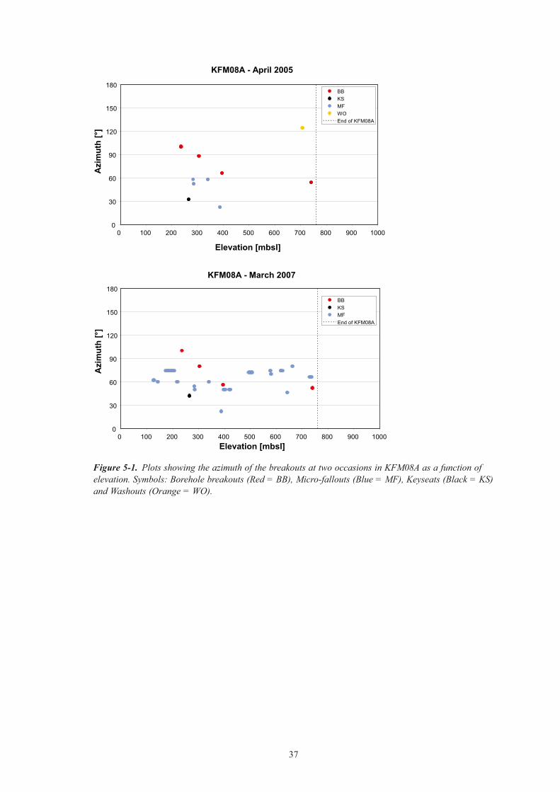
Figure 5‑1. Plots showing the azimuth of the breakouts at two occasions in KFM08A as a function of elevation. Symbols: Borehole breakouts (Red = BB), Micro-fallouts (Blue = MF), Keyseats (Black = KS) and Washouts (Orange = WO).

KFM08A - April 2005

0

30

60

90

120

150

180

0 100 200 300 400 500 600 700 800 900 1000

Elevation [mbsl]

Azi

mut

h [°

]BBKSMFWOEnd of KFM08A

KFM08A - March 2007

0

30

60

90

120

150

180

0 100 200 300 400 500 600 700 800 900 1000Elevation [mbsl]

Azi

mut

h [°

]

BBKSMFEnd of KFM08A

38

Figure 5‑2. Plots showing the azimuth of the breakouts in KFM08C, KFM09A and KFM09B as a function of elevation. Symbols: Borehole breakouts (Red = BB), Micro-fallouts (Blue = MF), Keyseats (Black = KS) and Washouts (Orange = WO).

KFM08C

0

30

60

90

120

150

180

0 100 200 300 400 500 600 700 800 900 1000

Elevation [mbsl]

Azi

mut

h [°

]

BBKSMFEnd of KFM08C

KFM09A

0

30

60

90

120

150

180

0 100 200 300 400 500 600 700 800 900 1000Elevation [mbsl]

Azi

mut

h [°

]

BBMFWOEnd of KFM09A

KFM09B

0

30

60

90

120

150

180

0 100 200 300 400 500 600 700 800 900 1000Elevation [mbsl]

Azi

mut

h [°

]

BBMFWOEnd of KFM09B

39

Figure 5‑3. Rose diagram showing the orientation of the “classical” breakouts not associated with structures in boreholes KFM08A (March 2007), KFM08C, KFM09A and KFM09B. There were 9 borehole breakouts.

Figure 5‑4. Rose diagram showing the orientation of micro-fallouts not associated with structures in boreholes KFM08A (March 2007), KFM08C, KFM09A and KFM09B. There were 31 micro-fallouts.

Figure 5‑5. Rose diagram showing the orientation of keyseats not associated with structures in boreholes KFM08A (March 2007), KFM08C, KFM09A and KFM09B. There were 2 keyseats.

40

5.1.3 Compilation of breakout data for all boreholesThese plots are based on data from Sicada and includes boreholes KFM01A, KFM01B, KFM02A, KFM03A, KFM04A, KFM05A, KFM06A, KFM07C, KFM08A (March 2007), KFM08C, KFM09A and KFM09B.

Borehole breakouts (BB)

In Figure 5­6 two rose­diagrams shows the variation in median value depending on if only breakouts (BB) associated with structures are shown or if all breakouts (BB) are shown.

Figure 5­7 shows breakouts (BB) (inclusive associated with structures) at 4 different elevation intervals, 0–150 m, 150–300 m, 300–400 m and >400 m, and Figure 5­8 shows the same type of diagrams but only for breakouts not associated with structures. No main difference in the preferred orientation can be seen. The orientation of the breakouts is consistently NE­SW, thus indicating a minor horizontal stress in this direction.

Micro-fallouts (MF)

In Figure 5­9 the rose­diagrams show the variation for micro­fallouts (MF). The difference depending on whether fallout associated with structures is included or not is only 2 degrees. The median orientation of micro­fallouts roughly coincides with the orientation for borehole breakouts (BB).

Figure 5­10 and Figure 5­11 shows micro­fallouts (MF) associated respectively micro­fallouts not associated with structures and not at four different elevation intervals, 0–150, 150–300, 300–400 and >400 m. As for the breakouts, no main shift in orientation with depth for the micro­fallouts may be observed.

Figure 5‑6. Rose diagram showing the orientation of the “classical” breakouts in boreholes KFM01A, KFM01B, KFM02A, KFM03A, KFM04A, KFM05A, KFM06A, KFM07C, KFM08A (March 2007), KFM08C, KFM09A and KFM09B. In the left rose diagram all BB (142 breakouts) are shown and in the right only breakouts not associated with structures are shown (42 breakouts).

41

Figure 5‑7. Rose diagram showing the orientation of the “classical” breakouts at different depth in boreholes KFM01A, KFM01B, KFM02A, KFM03A, KFM04A, KFM05A, KFM06A, KFM07C, KFM08A, KFM08C, KFM09A and KFM09B. The number of breakouts is 11 in the interval 0–150 m, 27 between 150–300 m, 29 between 300–400 and 75 for depths >400 m. See also Figure 5-8 for the breakouts that are not associated with fractures.

0-150 m 150-300 m

300-400 m >400 m

42

Figure 5‑8. Rose diagram showing the orientation of the “classical” breakouts not associated with structures at different depth in boreholes KFM01A, KFM01B, KFM02A, KFM03A, KFM04A, KFM05A, KFM06A, KFM07C, KFM08A, KFM08C, KFM09A and KFM09B. The number of breakouts is 5 in the interval 0–150 m, 8 between 150–300 m, 3 between 300–400 and 26 for depths >400 m.

0-150 m 150-300 m

300-400 m >400 m

43

Figure 5‑9. Rose diagram showing the orientation of the micro-fallouts (MF) in boreholes KFM01A, KFM01B, KFM02A, KFM03A, KFM04A, KFM05A, KFM06A, KFM07C, KFM08A (March 2007), KFM08C, KFM09A and KFM09B. In the left rose diagram all MF (85 micro-fallouts) are shown and in the right only breakouts not associated with structures are shown (64 micro-fallouts).

All MF MF not associated with structures

Median = 58°Median = 60°

44

0-150 m 150-300 m

300-400 m >400 m

Figure 5‑10. Rose diagram showing the orientation of the micro-fallouts associated with structures at different depth in boreholes KFM01A, KFM01B, KFM02A, KFM03A, KFM04A, KFM05A, KFM06A, KFM07C, KFM08A, KFM08C, KFM09A and KFM09B. The number of micro-fallouts is 11 in the interval 0–150 m, 20 between 150–300 m, 17 between 300–400 and 41 at depths >400 m. See also Figure 5-11 for the micro-fallouts that are not associated with fractures.

45

5.2 SummaryThe frequency and orientation of the occurrence of classical breakouts and micro­fallouts in the boreholes included in the additional study (KFM08A, KFM08C, KFM09A and KFM09B) are fairly similar to the previously results reported by /Martin 2007/.

The proportion of the total borehole length consisting of “classical” borehole breakouts varies from 0.2% in KFM03B to 5.6% in KFM02A among all the studied boreholes at Forsmark. (With “classical” breakout is meant a breakout with obvious diametrically opposite deep fallouts /Ringgaard 2007a/.)

In the additionally studied, as well as in the previously studied boreholes /Martin 2007/, there is no observed increase in the frequency of occurrence of borehole breakouts or micro­fallouts with depth.

Figure 5‑11. Rose diagram showing the orientation of the micro-fallouts not associated with structures at different depths in boreholes KFM01A, KFM01B, KFM02A, KFM03A, KFM04A, KFM05A, KFM06A, KFM07C, KFM08A, KFM08C, KFM09A and KFM09B. The number of micro-fallouts is 8 in the interval 0–150 m, 12 between 150–300 m,12 between 300–400 and 34 at depths >400 m.

0-150 m 150-300 m

300-400 m >400 m

46

The mean orientation from the mean azimuth of the borehole breakouts is about 48° at drill site 8 and about 73° at drill site 9. This implies that the orientation of the major horizontal stress may be slightly different at the two sites, 138° and 163°, respectively. The previously studied boreholes show a similar variation for the mean breakout azimuth, from 47° as the lowest value (in KFM03) to 78° as the highest value (in KFM02).

No new “classical” borehole breakouts could be observed in KFM08A at the repeated measure­ments, which indicate that there has been no significant ongoing borehole wall failure during this two year period.

The difference in azimuth for the four borehole breakouts in borehole KFM08A, which was measured repeatedly (in April 2005 and March 2007) is between 0° and 10°. Although the different measurements were made by different televiewer resolutions, the length (i.e. involving a large amount of measurement values along the breakout section) of most breakouts is enough that this difference may be regarded as a rough indication on the accuracy of breakout azimuth measurements.

5.3 Visualisation of the in situ stress dataVisualisation of the in situ stress data in Sicada using RVS has been carried out as a support for the illustration of the spatial location of available data and for the study of the influence of geological structures on the measured stresses.

5.3.1 Overcoring stress measurements Data were extracted from Sicada (delivery 08_029), /Carlsson and Olsson 1982/ and /Sjöberg 2004/, see Table 5­3. For KFK001 and KFK003 (previously called DBT1 and DBT3), data were taken from /Carlsson and Olsson 1982/, since these data are considered to have a higher reli­ability regarding the elastic modulus /Christiansson 2008, Sjöberg et al. 2005/ than the original calculations /Ingevald and Strindell 1981/, which are the values presently contained in Sicada.

The RVS visualizations make use of the RVS stress tensor tool. The principal stress components are plotted according to the convention in Table 5­4.

Table 5‑3. Sources of the overcoring data used for RVS visualization.

Borehole Source North reference

KFK001, KFK003 Carlsson & Olsson, 1982 Magnetic northKFM01B Sicada 08_029

Average values from P-04-83 table 5-10RT90/RHB70

KFM02B, KFM07B, KFM07C Sicada 08_029 RT90/RHB70

Table 5‑4. Colour codes for visualization of the principal stress magnitudes.

Stress component Symbol Colour

Major principal stress s1 Red

Intermediate principal stress s2 Green

Minor principal stress s3 Blue

Note: Tensile stresses (σ < 0) are marked with a dot at the end of the tensor component.

47

For all tensor components, the magnitude is presented with a certain scale factor (m/MPa) with respect to the value of the principal stress. The orientation of the tensors refers to RT90­RHB70 coordinate system. The same reference system was also used for the case of KFK001 and ­003 despite the data in reality refers to the magnetic north. Strictly speaking, the orientations of the measurements in KFK­boreholes and those in KFM­boreholes cannot be directly compared. In fact, the magnetic north varies both in time and space. Up to now, there is no function in RVS that corrects the orientations although this is technically possible. The difference between geographical and magnetic north can be estimated to be at most 10º.

In the following figures (Figure 5­12 to Figure 5­14), the average values for each measurement level are shown in relation to selected deformation zones and fracture domains. A legend of the illustrations is presented below.

The length of the tensor components are represented by a scale factor (m/MPa). Negative values are marked with a dot at the end of the tensor component.

Figure 5‑12. Results from overcoring measurements shown as tensor components in relation to fracture domains and deformation zones in Forsmark 2.2 local model volume as average magnitudes for each measured section. The orientations in the KFK-boreholes refer to magnetic north and cannot be directly compared with the orientations in the KFM-holes which refer to RT90-RHB70 north. View from W.

Figure 5‑13. Results from overcoring measurements shown as tensor components in relation to fracture domains and deformation zones in Forsmark 2.2 local model volume as average magnitudes for each measured section. The orientations in the KFK-boreholes refer to magnetic north and cannot be directly compared with the orientations in the KFM-holes which refer to RT90-RHB70 north. View from N-E.

48

5.3.2 Hydro‑fracturing stress measurementsThe location of the hydro­fracturing in situ stress measurements (HF and HTPF measurements) performed in Forsmark stage 2.2 and contained in Sicada (delivery 08_029 and 08_085) are shown in Figure 5­15. The locations of the measurements along the boreholes are marked with a disc in green colour for successful measurements and red colour for the measurements that failed (result not included in Sicada).

5.3.3 SummaryVisualisation of the in situ stress data in Sicada using RVS give a good overview of where the measurements are located in relation to fracture domains and deformation zones, whereas the plots showing the stress tensor from the overcore measurements are more difficult to grasp. However, the tensor plots visualize large differences in stress magnitudes and measured stress orientation relatively well. The complied RVS plots support the previous interpreted stress model presented by modelling stage 2.2 /Glamheden et al. 2007a/.

Figure 5‑14. Results from overcoring measurements shown as tensor components in relation to fracture domains and deformation zones in Forsmark 2.2 local model volume. The average magnitudes for each measured section are presented in a view from the top. The orientations in the KFK-boreholes refer to magnetic north and cannot be directly compared with the orientations in the KFM-holes which refer to RT90-RHB70 north.

49

5.4 Stress variability with depth due to varying modulus5.4.1 BackgroundAt the Forsmark site, seismic investigations show a gradual increase in seismic P­wave velocity with depth /Juhlin et al. 2002/. Within the first 100 m, the velocity of the P­wave is significantly lower than for the rock situated deeper. Indirectly, it is possible to obtain approximate values of the deformation modulus of the rock mass, as this property may be related to the P­wave and S­wave velocity from a seismic profile.

During modelling stage 2.2, numerical simulations were carried out with a stepwise increase in Young’s modulus estimated based on measured P­wave velocity and evaluated dynamic shear modulus of the rock at the Forsmark site /Glamheden et al. 2007a/. The aim of this modelling was to study the influence of an increasing deformation modulus on the state of in situ stress with depth and to observe if a better agreement with the in situ stress measurement results could be deduced.

The analysis described below re­examines the already performed investigation with a different numerical code and serves as an update of the previous work. The present model incorporate adjusted values for the deformation modulus that are higher than those used in modelling stage 2.2, see Table 5­5. The values used in the previous study were proportional to the dynamic shear modulus of the rock mass, while the values used here were related to the estimated rock mass properties for the different fracture domains based on the empirical and theoretical model­ling of the rock mass mechanical properties /Glamheden et al. 2007a/.

5.4.2 Input data and model set‑upA numerical model was set­up using FLAC, a two­dimensional explicit finite difference code developed by the Itasca group /Itasca 2005/. In contrast to finite element codes FLAC may simulate the behaviour of continuum media, in this case a rock mass, prior to and after a pos­sible failure. However the present simulation was based on an entirely elastic model and a plain strain solution.

The geometry and the boundary conditions of the model are presented in Figure 5­16. The mesh is square shaped with a side length of 1,000 m. A fine uniform zoning was used where the mesh size was 10 m. The bottom of the model was fixed in vertical direction, whereas the top bound­ary (ground surface) was free from any restraint. The so called ‘tectonic push’ was simulated by forcing the vertical boundaries of the model block to move inwardly at a very low velocity.

Figure 5‑15. Location of the hydro-fracturing in situ stress measurements (HF and HTPF) in relation to fracture domains and deformation zones in Forsmark 2.2 local model volume. View from S-W. Green discs represent successful measurements while red discs the measurements that failed (results not included in Sicada).

50

The deformation modulus of fracture domain FFM01 and FFM06 within the target volume was estimated to 70 GPa based on the empirical and theoretical modelling. The deformation modulus of FFM02 was estimated to 55 GPa, based on the empirical modelling /Glamheden et al. 2007a/. The relative change of Young’s modulus of the rock mass within the fracture domain FFM01 was estimated from the P­wave velocity /Juhlin et al. 2002/. Table 5­5 presents the values of Young’s modulus that were used in the present numerical model and for comparison also the values used by modelling stage 2.2.

It is to be noted that the division of the rock mass into regular blocks with clear border lines and the inter­block abrupt changes in Young’s modulus is a simplification of the real case, where the limits may follow any natural structure or pattern that exists in the rock mass. For example, the calculated Young’s modulus of 55 GPa, associated with fracture domain FFM02, is taken to represent the rock mass above a depth of 150 m in the numerical model, whereas the fracture domain itself is formed as an elongated wedge­shaped body of shallow rock that varies in thickness. The advantage of such simplification is in the clarity with which the effect of a non­gradual variation of the Young’s modulus on state of in situ stress can be studied.

Table 5‑5. P‑wave velocity and evaluated dynamic shear modulus together with Young’s modulus estimated during modelling stage 2.2 and 2.3 for associated depth intervals.

Depth interval [m] Vp3) [m/s] Gd

3) [GPa] Young’s modulus [GPa]Modelling stage 2.2 Modelling stage 2.3

0 – 1501) 4,800 – 5,800 20–30 35 55150 – 3002) 5,800 – 6,000 30–32 38 65300 – 4002) 6,000 – 6,100 32–33 45 65400 – 10002) 6,100 – 6,400 33–35 58 70

1) Fracture domain FFM02. 2) Fracture domain FFM01 and FFM06. 3) Based on Figure 6-7 in /Glamheden et al. 2007a/.

Figure 5‑16. Geometry and the boundary conditions of the used model The yellow lines mark the positions there Young’s modulus are changed.

150 m

400 m

1000 m

1000 m

150 m

400 m

1000 m

1000 m1000 m

51

Prior to a simulation run, the model is pre­conditioned to bear an initial isotropic stress field (σv = σH ) with the stress magnitude equivalent to gravitational loading. As soon as analysis begins, the inward movement of the two vertical boundaries brings about a new stress field, which is influenced by the initial stress field as well as by Poisson’s ratio. A simulation run is halted and re­started a number of times in order to examine the closeness of the prevailing stresses against “target stress values”. Target stress values were chosen from the in situ stress measurements, carried out in boreholes. The simulation run is terminated when the simulated stress magnitudes are similar to the measured in situ stresses.

5.4.3 ResultsFigure5-17showsthestepwisevariationinthenumericallycalculatedmajorprincipalstress,σ1, with depth. The two abrupt and significant deviations from the otherwise gradually increasing σ1 values are associated with the limits where the rock mass deformation moduli change. In situ stress measurements, carried out by the overcoring method in boreholes KFK001 (DBT1), KFK003 (DBT3), KFM02B and KFM07C are plotted in the figure for comparison.

Figure 5‑17. Estimated major principal stress, σ1, versus depth from the numerical analysis. Measured stresses by overcoring methods from boreholes KFK001 (DBT1), KFK003 (DBT3), KFM02B and KFM07C are added to the plot for comparison.

52

5.4.4 SummaryApart from differences in the absolute stress magnitude, this study produces result that are similar to those obtain in the study performed in modelling stage 2.2 /Glamheden et al. 2007a/. The results in both studies indicate a gradual increase of the in situ stress magnitude that is in reasonable agreement with the observed state of in situ stress. However, the measured data indicate larger variation in the in situ stresses with depth than possible to achieve in the model using the rock mass deformation properties evaluated by the empirical and theoretical approach. Furthermore, the current study results in shifting of the in situ stresses towards higher magnitude and actually less agreement with the measured data than the previous study.

A possible reason for the divergence between the measured and calculated stress variability with depth is differences in the rock mass volume that is involved in the various estimations. The volume involved in the stress measurements is approximately 0.05 m3. The deformation properties included in the numerical model are evaluated from observations in boreholes of 5 m sections (i.e. local heterogeneity is not studied), and the seismic measurements presented here cover a 16 km long survey. The seismic measurements consequently present the conditions of the rock mass mainly in a regional scale, the empirical and theoretical approach presents the conditions in a local scale and the stress measurements are based on point observations.

Fracture frequency decreases with depth and therefore the stiffness (Young’s modulus) must increase with depth. Matching stress magnitudes with stress measurements is simply a function of the assumptions used and the applied boundary conditions. The modelling was not an attempt to match the measured stresses but to illustrate the concept that a simple modulus increase with depth may explain the stress increase with depth.

53

6 Summary

6.1 Intact rock propertiesIn this modelling stage, additional samples were collected in fracture domain FFM06. Testing of these samples confirms the results from modelling stage 2.2 where the albitized variants of metagranite (101057) and aplitic granite (101058) in FFM06 are shown to be stiffer and stronger than the intact rock in fracture domain FFM01. However, the albitization does not seem to have any effect of the tensile strength of tested rock types.

The tests performed on samples composed of sealed fracture networks from ZFMENE0060A show results close to those obtained on intact rock from FFM01. The sealed fractures seem to have an insignificant influence of the mechanical properties of intact rock.

The latest results from the microcrack volume measurements confirm the previous test results. The samples from KFM01A show a clear linear increase of the microcrack volume strain with depth, while the samples from KFM02B display minor variation with depth.

Test results on intact rock samples as well as stochastic modelling of the variability of uniaxial compressive strength show that rock domain RFM045 displays greater variability and has a larger proportion of rock with low compressive strength (< 150 MPa) than domain RFM029. In both domains, the lower values of the compressive strength depend on mainly amphibolite (102017) and tonalitic varieties of granodiorite to tonalite (101051).

6.2 Rock mass propertiesThe characterization of the Singö and Forsmark deformation zone returns rock mass qualities that ranges from fair rock to excellent rock quality. The mode and mean value of the character­ized borehole sections correspond to “good rock” quality. Compared to the major, minor and possible deformation zones characterized in the target volume, the Singö and the Forsmark deformations zone show less variation of the rock mass quality, i.e. the lowest and highest rock mass quality has been observed in other deformations zones in the target volume. Possibly, this can also be due to particular conditions at the location of the analysed boreholes.

The mechanical properties estimated for the Singö deformation zone based on the empirical mod­elling presented here indicate a stiffer and stronger rock mass than the estimations based on back­calculation from displacements measurements in the SFR­tunnel passage of the Singö deformation zone presented by /Glamheden et al. 2007b/. The most conceivable reason for the difference in the estimated rock mass properties is simply that the deformation zone has a heterogeneous nature, which is supported by observation in the various access tunnels through the deformation zone.

The mechanical properties of the deformations zones for use in the regional stress modelling were based on the theoretical approach /Glamheden et al. 2007a/, which displays lower stiffness and strength than the properties calculated based on the empirical methods.

6.3 In situ state of stressThe frequency and orientation of the occurrence of “classical” breakouts and micro­fallouts in the boreholes included in this additional study (KFM08A, KFM08C, KFM09A and KFM09B) are fairly similar to the previously results reported by /Martin 2007/ and support the stress model presented in modelling stage 2.2 /Glamheden et al. 2007a/. In the additionally studied, as well as in the previously studied boreholes, there is no observed increase in the frequency of occurrence of borehole breakouts or micro­fallouts with depth.

54

Visualization of the in situ stress data is an excellent way to get an overview of the measurements locations in relation to fracture domains and deformation zones. The complied plots in this report support the interpreted stress model presented by modelling stage 2.2 /Glamheden et al. 2007a/.

A new model based on a finite difference code was run in order to further study the influence on in situ stresses of an increasing Young’s modulus towards depth. This modelling indicates a gradual increase of the in situ stress magnitude that is in reasonable agreement with the observed state of in situ stress. However, the measured data indicate larger variation in the in situ stresses with depth than possible to achieve in the model using the rock mass deformation properties evaluated by the empirical and theoretical approach. Furthermore, the current study results in shifting of the in situ stresses towards higher magnitude and actually less agreement with the measured data than the previous numerical modelling presented in stage 2.2. However the aim of the modelling in stage 2.3 was to confirm the influence of an improvement in rock mass quality with depth on the in situ stress. As such, local heterogeneities and geological structures were not modelled, which influence the absolute magnitude and variability of the in situ stresses measured in the model.

55

7 References

Andersson J, Christiansson R, Hudson J, 2002. Site investigations. Strategy for Rock Mechanics Site Descriptive Model. SKB TR­02­01, Svensk Kärnbränslehantering AB.

Back P-E, Sundberg J, 2007. Thermal Site Descriptive Model. A Strategy for the Model Development during Site Investigations. Version 2.0. SKB R­07­42, Svensk Kärnbränslehantering AB.

Back P E, Wrafter J, Sundberg J, Rosén L, 2007. Thermal properties. Site descriptive modelling Forsmark – stage 2.2. SKB R­07­47, Svensk Kärnbränslehantering AB.

Carlsson A, Olsson T, 1982. Characterization of deep­seated rock masses by means of borehole investigations. In situ rock stress measurements, hydraulic testing and core­logging. Final Report, April 1982, Research and Development Report 5:1. The Swedish State Power Board.

Dehlin P, 1983. Unpublished results from laboratory tests of samples collected at SFR. Royal Institute of Technology. (In Swedish.)

Christiansson R, 2008. Personal communication, SKB 2008­04­24.

Deutsch C, Journel A, 1998. GS­LIB: Geostatistical Software Library and User’s Guide. Second edition. Oxford University Press, New York.

Glamheden R, Fredriksson A, Persson P, Röshoff K, Karlsson J, Hakami H, Christiansson R, 2007a. Rock mechanics – Site descriptive modelling Forsmark stage 2.2. SKB R­07­31, Svensk Kärnbränslehantering AB.

Glamheden R, Hansen L M, Fredriksson A, Bergkvist L, Markström I, Elfström M, 2007b. Mechanical modelling of the Singö deformation zone – Site descriptive modelling Forsmark stage 2.1. SKB R­07­06, Svensk Kärnbränslehantering AB.

Hoek E, Brown E T, 1980. Underground excavations in rock.

Ingevald K, Strindell L, 1981. Rock stress measurments in deep vertical boreholes. Swedish State Power Board. Report L­543:2. (In Swedish.)

Itasca, 2005. Fast Lagrangian Analysis of Continua (FLAC), User’s guide. Itasca consulting group, Inc., Minneapolis.

Jacobsson L, 2007a. Borehole KFM06A. Uniaxial compression test of intact rock containing sealed fractures. Forsmark site investigation. SKB P­07­207, Svensk Kärnbränslehantering AB.

Jacobsson L, 2007b. Borehole KFM08D. Uniaxial compression test of intact rock. Forsmark site investigation. SKB P­07­145, Svensk Kärnbränslehantering AB.

Jacobsson L, 2007c. Borehole KFM08D. Indirect tensile strength test. Forsmark site investigation. SKB P­07­146, Svensk Kärnbränslehantering AB.

Jacobsson L, 2007d. Boreholes KFM01A and KFM02B. Microcrack volume measurements and triaxial compression tests on intact rock. Forsmark site investigation. SKB P­07­93, Svensk Kärnbränslehantering AB.

Jacobsson L, 2007e. Borehole KFM01C. Uniaxial compression test of intact rock. Forsmark site investigation. SKB P­06­69, Svensk Kärnbränslehantering AB.

Juhlin C, Bergman B, Palm H, 2002. Reflection seismic studies in the Forsmark area – stage 1. SKB R­02­43, Svensk Kärnbränslehantering AB.

56

Martin C D, Stimpson, B, 1994. The effect of sample disturbance on laboratory properties of Lac du Bonnet granite. Canadian Geotechnical Journal, vol. 31, pp 692–702.

Martin C D, 2007. Quantifying in situ stress magnitudes and orientations for Forsmark, Forsmark stage 2.2. SKB R­07­26, Svensk Kärnbränslehantering AB.

Martin C D, Christiansson R, Söderhäll J, 2001. Rock stability considerations for siting and constructing a KBS­3 repository. Based on experiences from Äspö HRL, AECL’s URL, tunnelling and mining. SKB TR­01­38, Svensk Kärnbränslehantering AB.

Ringgaard J, 2007a. Forsmark site investigation, mapping of borehole breakouts, processing of acoustical televiewerdata from KFM08A, KFM08C, KFM09A, KFM09A, KFM09B and KFM90B. SKB P­07­166, Svensk Kärnbränslehantering AB.

Ringgaard J, 2007b. Mapping of borehole breakouts, processing of acoustical televiewerdata from KFM01A, KFM01B, KFM02A, KFM03A, KFM03B, KFM04A, KFM05A, KFM06A and KFM07C. SKB P­07­07, Svensk Kärnbränslehantering AB.

Röshoff K, Lanaro F, Jing L, 2002. Strategy for a Rock Mechanics Site Descriptive Model. Development and testing of the empirical approach. SKB R­02­01, Svensk Kärnbränslehantering AB.

Sjöberg J, 2004. Overcoring rock stress measurements in borehole KFM01B. Forsmark site investigation. SKB P­04­83, Svensk Kärnbränslehantering AB.

Sjöberg J, Lindfors U, Perman F, Ask D, 2005. Evaluation of the stress at the Forsmark site. Preliminary site investigation Forsmark area – version 1.2. SKB R­05­35, Svensk Kärnbränslehantering AB.

Stephens M B, Fox A, Isaksson H, Öhman J, Simeonov A, 2007. Geology – Site descriptive modelling, Forsmark stage 2.2. SKB R­07­45, Svensk Kärnbränslehantering AB.

Stille H, Fredriksson A, 1987. Measurements, calculations and stability prognoses at the SFR undersea repository for low – and medium – level nuclear waste. Proc. Rock Mechanics Meeting in Stockholm, pp 207–224. SveBeFo. (In Swedish.)

Stille H, Dehlin P, 1981. Unpublished results from laboratory tests of samples collected at SFR. Royal Institute of Technology. (In Swedish.)

Sundberg J, Back P-E, Bengtsson A, Ländell M, 2005. Thermal modelling of the Simpevarp area. Supporting document for thermal model version 1.2. SKB R­05­24, Svensk Kärnbränslehantering AB.

Sundberg J, Wrafter J, Ländell M, Back P-E, Rosén L, 2008. Thermal properties. Complementary site descriptive modelling Forsmark – stage 2.3. SKB R­08­65, Svensk Kärnbränslehantering AB.

Wrafter J, Sundberg J, Ländell M, Back P, 2006. Thermal modelling. Site descriptive modelling. Laxemar 2.1. SKB R­06­84, Svensk Kärnbränslehantering AB.

57

Appendix A

Simulation of UCSThis appendix presents the results of stochastic simulation of UCS for rock domains RFM029 and RFM045 following the methodology described in Chapter 3.

A.1 Assessment of UCS dataUniaxial compressive strength from measurements Test results of uniaxial compressive strength (UCS) in data freeze 2.3 are summarised for each rock type in Table A­1 irrespective of rock domain. Tests were performed on drill core samples taken from ten different boreholes.

The majority of the measurements were performed on the dominant granite to granodiorite (101057). Albitized granite to granodiorite (101057) is distinguished from unaltered varieties of the same rock type. It is obvious that the albitized variety, which occurs almost exclusively in rock domain RFM045, has a significantly higher compressive strength than the unaltered variety, characteristic of rock domain RFM029. Granite (101058), the dominant rock in domain RFM045, is also typically albitized /Stephens et al. 2007/. Samples of this rock also have rather high compressive strengths.

Due to the lack of samples of amphibolite (102017) within the target volume, UCS of amphibolite is based on data from SFR at Forsmark, located in rock domain RFM021 /Stille and Fredriksson 1987, Stille and Dehlin 1981, Dehlin 1983/.

Many of the samples were taken in clusters of 3 to 5 samples from the same 1–2 m length of borehole core. Declustering techniques were applied to evaluate possible bias which may be caused by such a sampling method. The standard deviations quoted above are a measure of the total variability in the sample data, and comprise the spatial variability of compressive strength within a rock type in addition to variability associated with the testing method.

Table A‑1. Measured uniaxial compressive strength (MPa) of different rock types in the Forsmark area.Rock type Mean Std dev. Min. Max. Number of samples

Granite to granodiorite, 101057 222 25 157 289 74Granite to granodiorite, (albitized) 101057 373 20 338 391 10Granodiorite and tonalite, 101051 187 40 143 228 8Granite, metamorphic, aplitic, 101058 310 58 229 372 5Amphibolite, 102017 145 29 117 212 11Tonalite to granodiorite, 101054 162 16 140 176 4Granodiorite, 101056 236 12 222 249 4Pegmatite, pegamatitic granite, 101061 213 39 153 285 16Granite, fine- to medium-grained, 111058 246 1

Note: The table includes samples from other rock domains than RFM029 and RFM045.

58

Uniaxial compressive strength versus densityDensity logging data may be used for two purposes:

1. to estimate UCS values for some rock types,

2. to determine the spatial correlation structure of UCS.

A relationship between density and thermal conductivity for igneous rocks has been observed both between rock types and within rock types at both Laxemar/Simpevarp /Sundberg et al. 2005, Wrafter et al. 2006/ and Forsmark /Back et al. 2007/.

The relationship between density and UCS for all investigated rock types is illustrated in Figure A­1(a). With the exception of pegmatite (101061) and some granite to granodiorite (101057), rock types with higher density have generally lower compressive strength. Since density is intimately related to mineral compositions, it is reasonable to suggest that mineral composition is an important controlling factor for UCS. It can be argued that this relationship should also be present within a rock type. However, the only rock types for which a relationship is clear are granodiorite to tonalite (101051) and tonalite to granodiorite (101054). For most other rock types, the density intervals are very small which makes it difficult to discern any cor­relation. As regards pegmatite, it is suggested here that grain contacts in this very coarse grained rock have a dominating influence on compressive strength, thereby reducing the effect of mineral composition.

If a relationship between compressive strength and density can be established for a specific rock type, then density logging data can be used to estimate the distribution of compressive strength. This is particularly useful when laboratory tests are few in number, as in the case of granodiorite to tonalite (101051). Previous studies have shown that rock type 101051 has a wide variety of compositions, from tonalite, through granodiorite to subordinate granite with densities ranging from 2,680 kg/m3 to 2,820 kg/m3 /Stephens et al. 2007, Back et al. 2007/. On a cross plot of density and UCS, it is obvious that only a restricted range of compositional types of granodiorite to tonalite (101051) are represented by the laboratory data. A relationship between density and compressive strength based on such few data is considered unreliable especially for the lower density varieties. Therefore, it was decided to combine rock types tonalite to graniodiorite (101054) and granodiorite (101056) with granodiorite to tonalite (101051) and to base a rela­tionship on values from all three rock types Figure A­1(b). This was considered reasonable since these rock types fall within the compositional range shown by granodiorite to tonalite (101051). A linear equation describes the relationship between these variables rather well.

Applied to borehole density logging data, this relationship can be used to estimate compressive strength of granodiorite to tonalite (101051) along continuous sections of boreholes. These results are described in Appendix A.4.

59

Figure A‑1. Cross plot of density and UCS for a) all rock types and b) selected rock types including granodiorite to tonalite (101051). Based on linear regression, the relationship used in this study as a model to describe granodiorite to tonalite (101051). For the purposes of modelling compressive strength from density loggings, it is assumed that the established relationship is valid within the density interval 2,640–2,850 kg/m³.

100

150

200

250

300

350

400

2500 2600 2700 2800 2900 3000

Density (kg/m3)

UC

S (M

Pa)

101051101054101056101057101058 + albitized 101057101061102017

a)

y = -0.715x + 2159.325R2 = 0.908

100

140

180

220

260

300

2650 2700 2750 2800 2850 2900

UC

S (M

Pa)

101051+101054+101056

Model: 101051+101054+101056

b)Density (kg/m3)

60

A.2 Stochastic simulation of lithologiesStochastic simulations of lithologies for rock domains RFM029 and RFM045 were performed as part of the thermal modelling stages 2.2 and 2.3 and are described in detail in the thermal modelling reports /Back et al. 2007/ and /Sundberg et al. 2008/, respectively. The output from the stochastic simulations of lithologies is used in the modelling of compressive strength. A summary is given below.

For the purpose of geological simulations, rock types with similar thermal and lithological properties were assigned to the same class. Consideration was taken of a rock type’s geological properties, such as mineral composition, mode of occurrence and age. Four TRCs were defined in each rock domain. Three TRCs are common to both domains. The classification of rock types into TRCs for domain RFM029 and domain RFM045 are presented in Table A­2 and Table A­3.

Table A‑2. Division of rock types into TRCs for domain RFM029. Proportions of different rock types and geological characteristics are according to /Stephens et al. 2007/ and proportions of TRCs are from /Sundberg et al. 2008/.

TRC Rock name/code Proportions from geological model v. 2.2 /Stephens et al. 2007/ (%)

Proportions of TRCs in output from lithological simulations (%)

Composition, mode of occurrence, etc.

57 Granite to granodiorite, 101057 74 78.9 Both felsic group B rocks. Dominating granites.Granite, aplitic, 101058 1

51 Granodiorite to tonalite, 101051 5 3.8 Felsic to more intermediate group A and C rocks.Felsic to intermediate volcanic

rock, 1030760.4

61 Pegmatite, pegmatitic granite, 101061

13 13.1 Both felsic group D. rocks. Late tectonic dykes, segregations, veins.Granite, 111058 2

17 Amphibolite, 102017 Diorite, quartz diorite and gabbro, 101033

4 4.2 Both mafic group B rocks. Dykes and small irregular bodies.

Table A‑3. Division of rock types into rock classes for domain RFM045. Proportions of different rock types and geological characteristics are according to /Stephens et al. 2007/ and proportions of TRCs are from lithological simulations described in /Sundberg et al. 2008/.

TRC Rock name/code Proportions from geological model v. 2.2 /Stephens et al. 2007/ (%)

Proportions of TRCs in output from lithological simulations (%)

Composition, mode of occurrence, etc.

58 Granite to granodiorite, 101057 18 72 Both felsic group B rocks. Dominating granites com-monly affected by albitization.

Granite, aplitic, 101058 49

51 Granodiorite to tonalite, 101051 9 9 Felsic to more intermediate group A and C rocks.Felsic to intermediate volcanic

rock, 1030761

61 Pegmatite, pegmatitic granite, 101061

14 13 Both felsic group D rocks. Late tectonic dykes, segrega-tions, veins Granite, 111058 1

17 Amphibolite, 102017 Diorite, quartz diorite and gabbro, 101033

6 6 Both mafic group B rocks. Dykes and small irregular bodies.

61

In order to capture the lithological and structural heterogeneity present within a rock domain, borehole sections were divided into more homogenous groups. Models were constructed for each group of boreholes, and separate simulations were performed for each group or “sub­domain”. Both domain RFM029 and RFM045 were modelled by two subdomains. The basis for these subdivisions are described in /Back et al. 2007/ and /Sundberg et al. 2008/.

The proportions of TRCs in the output of the lithological simulations are compared with proportions estimated by geologists /Stephens et al. 2007/ in Table A­2 and Table A­3. The proportions of subordinate rocks are somewhat lower than in the geological model. The main reasons for these discrepancies are: 1) slightly different sets of boreholes were used by the different modelling teams, 2) the borehole data was processed in different ways, and 3) in the case of subdomain B in domain RFM045, the way in which T­PROGS (the software used for lithological simulations) interpreted the borehole data has produced some error. The effect of these differences on the UCS model is judged to be small.

Stochastic simulations of geology were performed with a resolution of 1 m and a simulated rock volume of 50 x 50 x 50 m. One hundred realisations of geology for each rock domain were selected for the purpose of modelling UCS. Table A­4 shows the number of realisations representing the subdomains within each domain. The number of realisations selected for each subdomain reflects their volumetric importance, which was based on judgements made in consultation with the geological modelling team.

Visualizations of example geology realisations for domain RFM029 and domain RFM045 are presented in Appendix A.8.

Table A‑4. Geological realisations representing each subdomain. Brief description of geology, based on /Back et al. 2007, Sundberg et al. 2008/.

Rock domain Realisation interval Distinguishing features

RFM029Subdomain Internal 1 – 67 Dominated by lineation and elongate bodies of subordinate rocks.Subdomain Marginal 68 – 100 Dominated by foliation and flattened bodies of subordinate rocks.RFM045Subdomain A 1 – 67 Dominated by granitoids and small bodies of subordinate rocks.Subdomain B 68 – 100 Lithologically mixed with large bodies of mafic rock.

62

A.3 Spatial statistical models of UCSTwo types of model are required for each TRC: a statistical distribution model and a model describing spatial correlation or dependence. Statistical distribution models of UCS for each TRC at 0.1 m resolution are presented below.

Statistical distribution models – 0.1 m resolutionA statistical distribution model is fitted to the histogram of UCS for each TRC. This is per­formed by smoothing the histogram with the smoothing algorithm in the geostatistical software GSLIB /Deutsch and Journel 1998/. This algorithm uses a simulated annealing procedure that honours the sample statistics.

TRC 57TRC 57 is dominated by granite to granodiorite (101057) and makes up approximately 75% of rock domain RFM029. Data values (n=74) used to define TRC 57 are based on fresh samples of granite to granodiorite (101057), see Figure A­2. Albitized samples are excluded. The statistical distribution model for this TRC is based on smoothing of the data histogram; Figure A­2. Minimum and maximum values of compressive strength were set to 150 MPa and 320 MPa respectively, which is slightly outside the range of the observations. Based on studies of other granitoid rocks, values lower than 150 MPa are judged unlikely.

TRC 58TRC 58 makes up approximately two­thirds of the rock volume in domain RFM045. It is dominated by albitized granite (101058), but also comprises a significant proportion of albitized granite to granodiorite (101057). The latter is distinguished from non­albitized granite to granodiorite (101057) by its higher UCS values. A histogram of the available data (10 of 101057 and 5 of 101058) is shown in Figure A­3. The samples were taken in spatially clustered groups, so the representativity must be considered rather poor. Declustering has little effect on the mean or standard deviation. Therefore, the uncensored data set was used. Despite the low number of samples, it is clear that the relatively high UCS values distinguish this TRC clearly from other TRCs. A model based on smoothing of the data histogram with arbitrarily chosen min and max values of 200 MPa and 440 MPa is shown in Figure A­3. It should be said, however, that such a model is highly uncertain.

Figure A‑2. Left: Histogram and statistics of uniaxial compressive strength for TRC 57 based on labo-ratory measurements of drill core samples. Right: Statistical distribution model of uniaxial compressive strength for TRC 57 based on smoothing of the data histogram.

63

TRC 61TRC 61, which comprises pegmatite and pegmatitic granite (101061) and granite (111058), makes up approximately 15% of the rock mass in both domains RFM029 and RFM045. Pegmatite (101061) is the dominant rock type in this class. A histogram of the 17 data values, 16 of which are pegmatite (101061), is shown in Figure A­4. The statistical distribution model based on smoothing of the data histogram is shown in Figure A­4. Minimum and maximum values of compressive strength were set to 130 MPa and 320 MPa respectively, which is slightly outside the range of the observations. Again, there is quite a high degree of uncertainty in the model.

TRC 17TRC 17 is dominated by amphibolite (102017) which occurs as a minor rock in both domains RFM029 and RFM045. A histogram of the available data (n=11) is shown in Figure A­5. The samples were taken in spatially clustered groups so the representativity must be considered rather poor. Declustering has little effect on the mean or standard deviation. Therefore, the uncensored data set was used. Despite the low number of samples, it can be stated that the relatively low UCS values distinguishes this TRC clearly from other TRCs. A model based on smoothing of the data histogram with min and max values of 100 MPa and 240 MPa is proposed; see Figure A­5. A distribution model based on such few data is naturally highly uncertain.

Figure A‑3. Left: Histogram and statistics of uniaxial compressive strength for TRC 58 based on labo-ratory measurements of drill core samples. Right: Statistical distribution model of uniaxial compressive strength for TRC 58 based on smoothing of the data histogram.

Figure A‑4. Left: Histogram and statistics of uniaxial compressive strength for TRC 61 based on labo-ratory measurements of drill core samples. Right: Statistical distribution model of uniaxial compressive strength for TRC 61 based on smoothing of the data histogram.

64

TRC 51TRC 51 is dominated by rock type granodiorite to tonalite (101051), and is present in both domain RFM029 and domain RFM045. A relationship between density and compressive strength was established for this rock type in section A.1. This relationship can be used to calculate compressive strength values from borehole density data, which is particularly useful in this case, since laboratory data are far too few to define reliable statistical distribution models Figure A­6. Borehole density logging data, recorded at 0.1 m intervals, indicates that this rock type comprises at least three distinct compositional variants, ranging from tonalite to granodiorite to subordinate granite. Therefore, it was decided to create three separate models, one for each compositional variety. This compositional variability has been recognised by the geological modelling team, although subdivision on the basis of density has not been attempted /Stephens et al. 2007/.

The borehole occurrences of rock type101051 were assigned to one of three groups based on their density ranges; see Table A­5. Individual bodies of this rock type are rather homogenous with respect to density. For each group, density logging values were used to calculate compressive strength based on the relationship referred to above. The distributions based on these calculations are associated with rather large uncertainties. Statistical distribution models of compressive strength for each variety are based on smoothing of these histograms (Figure A­7 to Figure A­9).

Figure A‑5. Left: Histogram and statistics of uniaxial compressive strength for TRC 17 based on labo-ratory measurements of drill core samples. Right: Statistical distribution model of uniaxial compressive strength for TRC 17 based on smoothing of the data histogram.

Figure A‑6. Histogram and statistics of uniaxial compressive strength data for granodiorite to tonalite (101051) based on laboratory measurements of drill core samples.

65

Table A‑5. Division of granodiorite to tonalite (101051) into subtypes based on density, and mean and standard deviation of UCS for each subtype. UCS calculated from density loggings using relationship defined in section A.1. Data was collected at 0.1 m intervals.

Grp A: low density (2,640–2,720 kg/m3)

Grp B: medium density (2,680–2,760 kg/m3)

Grp C: high density (> 2,750 kg/m3)

Mean 245 215 148

Std. dev. 13.1 14.2 16.9

Proportions of each subtype based on density logs

50% 30% 20%

Figure A‑7. Histogram of uniaxial compressive strength for TRC 51A based on calculations from density logs. Statistical distribution model based on smoothing of the data histogram. Minimum value = 210 MPa; maximum value = 270 MPa.

Figure A‑8. Histogram of uniaxial compressive strength for TRC 51B based on calculations from density logs. Statistical distribution model based on smoothing of the data histogram. Minimum value = 180 MPa; maximum value = 250 MPa.

66

A.4 Stochastic simulation of UCSFor each TRC, statistics of compressive strength based on results of the simulations are summa­rised in Table A­6. Statistics of the measured data are shown for comparison. The simulations at 0.1 m resolution have reproduced the means and standard deviations observed in the measured data. Table A­6 also shows the variance reduction after averaging within 1 m cubes.

The variogram models for the 1 m resolution are modified from the models used for the 0.1 m resolution according to the principles explained in /Back et al. 2007/ (Table A­7).

Table A‑6. Uniaxial compressive strength statistics for all simulated TRCs.

TRC Laboratory samples

0.1 m simulations 1m values1) Variance reduction2)

1m simulations3)

MPa MPa MPa % MPaMean St. dev. Mean St. dev. Mean St. dev. Mean St. dev.

17 145 29 145 29 145 22 42% 144 2051A 245 13 245 13 245 8 61% 245 851B 215 14 215 14 215 9 60% 215 851C 148 17 148 17 148 11 58% 147 1057 222 25 221 25 221 20 40% 221 1958 352 45 354 45 354 30 56% 353 2961 215 37 215 37 215 25 54% 215 23

1) A “1 m value” refers to the mean of all simulated 0.1 m values within a 1 m cube.2) Proportion by which the variance of 0.1 m values is reduced on averaging the 0.1 m values to 1 m values.3) Simulated values – 1 m resolution.

Figure A‑9. Histogram of uniaxial compressive strength for TRC 51C based on calculations from density logs. Statistical distribution model based on smoothing of the data histogram. Minimum value = 120 MPa; maximum value = 200 MPa.

67

Table A‑7. Variogram parameters for modelling at 1 m resolution for each TRC.

TRC Nugget Range Model

57 0 25 m Exponential58 0 3m/50 m Nested model: exponen tial/Gaussian 61 0 15 m Spherical51A 0 6 m Spherical51B 0 6 m Spherical51B 0 8 m Spherical17 0 25 m Spherical

A.5 Variogram model reproduction 1 m simulations

Figure A‑10. Comparison of the variogram model (blue line) and variograms from 5 independent realisations for different TRCs. Lag distance (x axis) in metres (m). Variogram is standardised to the variance of the simulated data. Horizontal black line corresponds to the sill of the variogram model.

68

Figure A‑11. Comparison of the variogram model (blue line) and variograms from 5 independent realisations for different TRCs. Lag distance (x axis) in metres (m). Variogram is standardised to the variance of the simulated data. Horizontal black line corresponds to the sill of the variogram model.

Figure A‑12. Histograms of simulation results of TRC 17 (left) and TRC 51A (right) at 1 m resolution based on 100 realisations.

A.6 Histograms of simulated UCS values for each TRCThe histograms below are based on simulated UCS values from 100 realisations of simulations with “1 m” resolution.

69

Figure A‑13. Histograms of simulation results of TRC 51B (left) and TRC 51C (right) at 1 m resolution based on 100 realisations.

Figure A‑14. Histograms of simulation results of TRC 57 (left) and TRC 58 (right) at 1 m resolution based on 100 realisations.

Figure A‑15. Histogram of simulation results of TRC 61 at 1 m resolution based on 100 realisations.

70

A.7 Visualisation of UCS realisations for each TRCIn this appendix, example realisations of compressive strength for each TRC are presented in 2D for simulations with a resolution of 1 m. All 2D­realisations represent a slice in the centre of a 3D cube. For example, the 25th slice of the xy­plane is the 25th slice that can be cut in the z­direction (there are 50 slices). Distance is in metres.

Figure A‑16. 2D slices from 3D realisations (resolution = 1 m) illustrating the distribution of compres-sive strength values (MPa) in TRC 17 and TRC 51A. Realisation=1, Slice=25, xy-plane. Distance is in metres.

Figure A‑17. 2D slices from 3D realisations (resolution = 1 m) illustrating the distribution of compres-sive strength values (MPa) in TRC 51B and TRC 51C. Realisation=1, Slice=25, xy-plane. Distance is in metres.

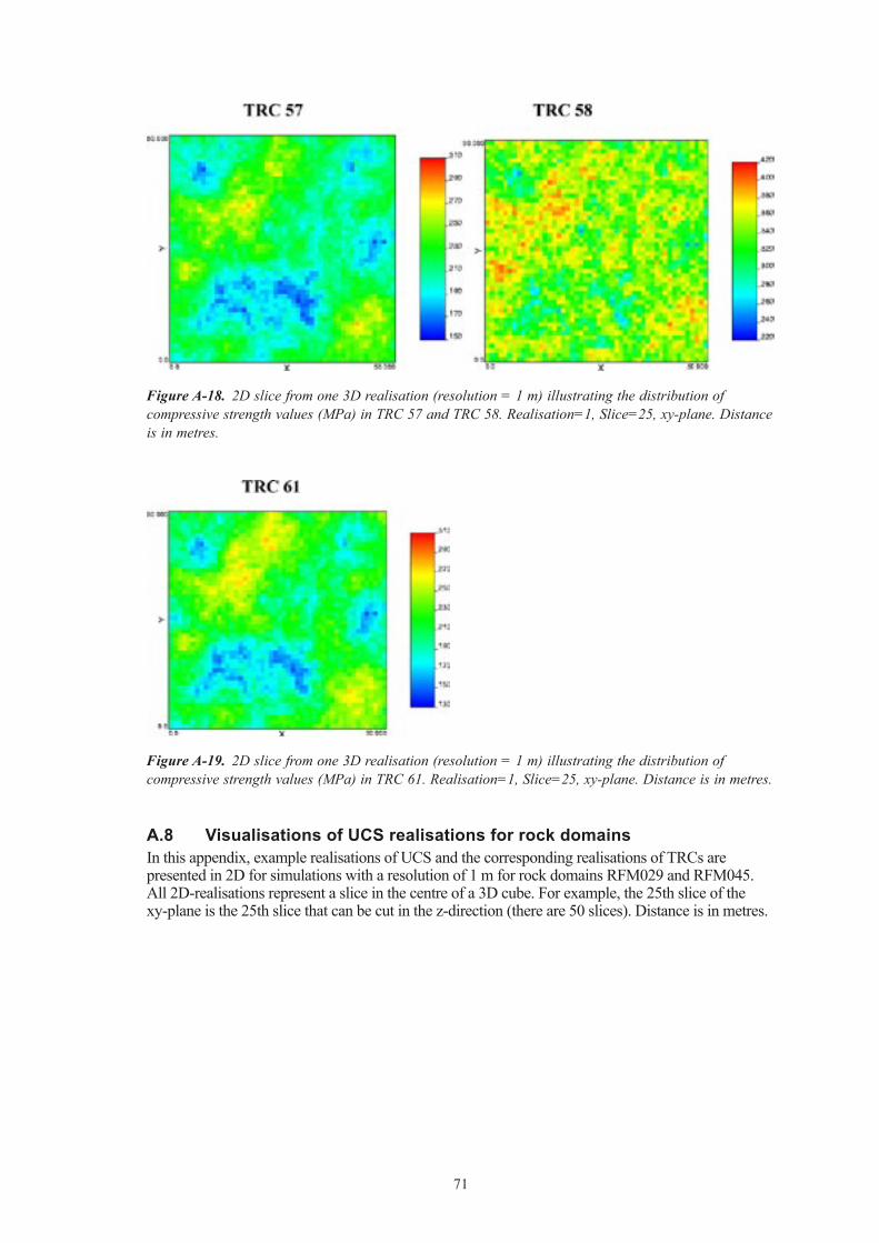
71

Figure A‑18. 2D slice from one 3D realisation (resolution = 1 m) illustrating the distribution of compressive strength values (MPa) in TRC 57 and TRC 58. Realisation=1, Slice=25, xy-plane. Distance is in metres.

Figure A‑19. 2D slice from one 3D realisation (resolution = 1 m) illustrating the distribution of compressive strength values (MPa) in TRC 61. Realisation=1, Slice=25, xy-plane. Distance is in metres.

A.8 Visualisations of UCS realisations for rock domainsIn this appendix, example realisations of UCS and the corresponding realisations of TRCs are presented in 2D for simulations with a resolution of 1 m for rock domains RFM029 and RFM045. All 2D­realisations represent a slice in the centre of a 3D cube. For example, the 25th slice of the xy­plane is the 25th slice that can be cut in the z­direction (there are 50 slices). Distance is in metres.

72

Figure A‑20. 2D slice from one 3D realisation (resolution = 1 m) illustrating the distribution of rock classes (left) and uniaxial compressive strength in MPa (right). Realisation = 1, Slice=25, xy-plane. Distance is in metres.

Figure A‑21. 2D slice from one 3D realisation (resolution = 1 m) illustrating the distribution of rock classes (left) and uniaxial compressive strength in MPa (right). Realisation = 1, Slice=25, yz-plane. Distance is in metres.

Figure A‑22. 2D slice from one 3D realisation (resolution = 1 m) illustrating the distribution of rock classes (left) and uniaxial compressive strength in MPa (right). Realisation = 1, Slice=25, xz-plane. Distance is in metres.

Domain RFM029

73

Domain RFM045

Figure A‑23. 2D slice from one 3D realisation (resolution = 1 m) illustrating the distribution of rock classes (left) and uniaxial compressive strength in MPa (right) in subdomain A1 – domain RFM045. Realisation = 1, Slice=25, xy-plane. Distance is in metres.

Figure A‑24. 2D slice from one 3D realisation (resolution = 1 m) illustrating the distribution of rock classes (left) and uniaxial compressive strength in MPa (right) in subdomain A1 – domain RFM045. Realisation = 1, Slice=25, xz-plane. Distance is in metres.

Figure A‑25. 2D slice from one 3D realisation (resolution = 1 m) illustrating the distribution of rock classes (left) and uniaxial compressive strength in MPa (right) in subdomain A1 – domain RFM045. Realisation = 1, Slice=25, yz-plane. Distance is in metres.

74

Figure A‑26. 2D slice from one 3D realisation (resolution = 1 m) illustrating the distribution of rock classes (left) and uniaxial compressive strength in MPa (right) in subdomain B – domain RFM045. Realisation = 1, Slice=25, xy-plane. Distance is in metres.

Figure A‑27. 2D slice from one 3D realisation (resolution = 1 m) illustrating the distribution of rock classes (left) and uniaxial compressive strength in MPa (right) in subdomain B – domain RFM045. Realisation = 1, Slice=25, xz-plane. Distance is in metres.

Figure A‑28. 2D slice from one 3D realisation (resolution = 1 m) illustrating the distribution of rock classes (left) and uniaxial compressive strength in MPa (right) in subdomain B – domain RFM045. Realisation = 1, Slice=25, yz-plane. Distance is in metres.

75

Appendix B

Results from empirical modellingB.1 Comparison of RMR and Q with fracture frequency

Figure B‑1. KFM11A. RMR and Q values obtained for characterization at 5 m sections along KFM11A. The minimum possible, mean, frequent and maximum possible values are shown. The horizontal lines represent the limit of the Singö deformation zone.

0

100

200

300

400

500

600

700

800

900

1000

20 40 60 80 100

Bor

ehol

e le

ngth

KFM11A-RMR-values

Minimum

Mean

Frequent

Maximum

Upper limit DZ

Lower limit DZ

0

100

200

300

400

500

600

700

800

900

1000

0 1 10 100 1000 10000

Bor

ehol

e le

ngth

KFM11A-Q-values

Minimum

Mean

Frequent

Maximum

Upper limit DZ

Lower limit DZ

76

Figure B‑2. KFM12A. RMR and Q values obtained for characterization at 5 m sections along KFM12A. The minimum possible, mean, frequent and maximum possible values are shown. The horizontal lines represent the limit of the Forsmark deformation zone.

0

50

100

150

200

250

300

350

400

450

500

20 40 60 80 100

Bor

ehol

e le

ngth

KFM12A-RMR-values

Minimum

Mean

Frequent

Maximum

Upper limit DZ

Lower limit DZ

0

50

100

150

200

250

300

350

400

450

500

0 1 10 100 1000 10000

Bor

ehol

e le

ngth

KFM12A-Q-values

Minimum

Mean

Frequent

Maximum

Upper limit DZ

Lower limit DZ

77

Figure B‑3. Comparison between mean RMR and mode Q values together with fracture frequency (fractures/m) obtained for characterization at 5 m sections along KFM11A and KFM12A, respectively. The fracture frequency is the sum of the fractures classified as open and partly open fractures.

0

100

200

300

400

500

600

700

800

900

10000 1 10 100 1000 10000

0

100

200

300

400

500

600

700

800

900

1000

0 25 50 75 100

Q

Bor

ehol

e le

ngth

RMR/ Fracture frequency (fractures/m)

Mean values from RMRFracture frequencyMode values from QUpper limit DZLower limit DZ

0 1 10 100 1000 10000

0

50

100

150

200

250

300

350

400

450

500

0 25 50 75 100

Q

Bor

ehol

e le

ngth

RMR/ Fracture frequency (fractures/m)

Mean values from RMRFracture frequencyMode values from QUpper limit DZLower limit DZ

KFM11A-Comparison KFM12A-Comparison

78

B.2 Variation of rock mass properties along the boreholes

Figure B‑4. KFM11A. Variation of the deformation modulus, uniaxial compressive strength, apparent friction angle and apparent cohesion of the rock mass with depth. The minimum, mean and maximum values are shown. The horizontal lines represent the limit of the Singö deformation zone.

0

100

200

300

400

500

600

700

800

900

1000

0 10 20 30 40 50 60 70 80 90 100

Bor

ehol

e le

ngth

[m]

KFM11A - Rock mass deformation modulus [GPa]

Max Em(RMR) Mean Em(RMR)

Min Em(RMR) Mean Em(Q)

Upper limit DZ Lower limit DZ

0

100

200

300

400

500

600

700

800

900

1000

0 20 40 60 80 100 120 140

Ber

ohol

e le

ngth

[m]

KFM11A - UCS of the rock mass [MPa]

Max UCS(RMR) Mean UCS(RMR)

Min UCS(RMR) Upper limit DZ

Lower limit DZ

0

100

200

300

400

500

600

700

800

900

1000

0 10 20 30 40

Bor

ehol

e le

ngth

[m]

Max c(RMR) Mean c(RMR) Min c(RMR)

Upper limit DZ Lower limit DZ

0

100

200

300

400

500

600

700

800

900

1000

0 10 20 30 40 50 60

Bor

ehol

e le

ngth

[m]

Max (RMR) Mean (RMR) Min (RMR)

Upper limit DZ Lower limit DZ

KFM11A - Apparent friction angle of the rock mass (Φ)[ º ](σ3=10-30 MPa)

KFM11A - Apparent cohesion of the rock mass [MPa](σ3=10-30 MPa)

79

Figure B‑5. KFM12A. Variation of the deformation modulus, uniaxial compressive strength, apparent friction angle and apparent cohesion of the rock mass with depth. The minimum, mean and maximum values are shown. The horizontal lines represent the limit of the Forsmark deformation zone.

0

50

100

150

200

250

300

350

400

450

500

Max Em(RMR) Mean Em(RMR)

Min Em(RMR) Mean Em(Q)

Upper limit DZ Lower limit DZ

0

50

100

150

200

250

300

350

400

450

500

Max UCS(RMR) Mean UCS(RMR)

Min UCS(RMR) Upper limit DZ

Lower limit DZ

0

50

100

150

200

250

300

350

400

450

500

Max c(RMR) Mean c(RMR)

Min c(RMR) Upper limit DZ

Lower limit DZ

0

50

100

150

200

250

300

350

400

450

500

Max (RMR) Mean (RMR) Min (RMR)

Upper limit DZ Lower limit DZ

0 10 20 30 40 50 60 70 80 90 100 0 20 40 60 80 100 120 140

0 10 20 30 400 10 20 30 40 50 60

Bor

ehol

e le

ngth

[m]

KFM12A - Rock mass deformation modulus [GPa]

Ber

ohol

e le

ngth

[m]

KFM12A - UCS of the rock mass [MPa]

Bor

ehol

e le

ngth

[m]

Bor

ehol

e le

ngth

[m]

KFM12A - Apparent friction angle of the rock mass (Φ)[ º ](σ3=10-30 MPa)

KFM12A - Apparent cohesion of the rock mass [MPa](σ3=10-30 MPa)

81

Appendix C

Data delivery from SicadaThe date of delivery of the input data from Sicada in the rock mechanics modelling is presented in Table C­1.

Table C‑1. Date of delivery of input data from Sicada in the rock mechanics modelling.

Parameter Activity Sicada delivery Date of delivery from Sicada

Dir_sheartest_sealed RM117 – Shear test Sicada-07-028 (0:1) 2007-02-09Dir_shear test_open RM117– shear test Sicada-07-028 (0:1) 2007-02-09Tilt_test RM118 – Tilt test Sicada-07-028 (0:2) 2007-02-09Strength_uniaxial RM113 – Strength_uniaxial Sicada-06-239 2006-10-06Strength_uniaxial Poisson_and_young

RM113 – Poisson_and_young Sicada_06-239 2006-10-06

Strength_triaxial RM115 – Strength_triaxial Sicada_06-239 2006-10-06Strength_triaxial Poisson_and_young

RM115 – Poisson_and_young Sicada_06-239 2006-10-06

Tensile Strength brazil_test RM110 – Tensile Strength brazil_test Sicada_06-239 2006-10-06P-wave RM100 – P-wave Sicada_06-239 2006-10-06KFM01A GE041 and GE300 Sicada_03_76 2003-08-12KFM02A GE041 and GE300 Sicada_04_17 2004-01-22KFM03A GE041 and GE300 Sicada_04_46 and

Sicada_04_682004-03-05 and 2004-04-01

KFM04A GE041 and GE300 Sicada_04_117 2004-05-25KFM01B, KFM09A, KFM09B GE041 and GE300 Sicada_06_134_1 2006-07-21KFM07C GE041 and GE300 Sicada_07_002 2007-01-03KFM06A, KFM06C KFM08C

GE041 and GE300 Sicada_07_156 2007-04-03

KFM11A, KFM12A GE041 and GE300 Sicada_07_444 2007-12-04Tensile Strength brazil_test RM110 – Tensile Strength brazil_test Sicada_08_033 2008-02-12Strength_uniaxial RM113 – Strength_uniaxial Sicada-08_033 2008-02-12Strength_uniaxial Poisson_and_young

RM113 – Poisson_and_young Sicada_08_033 2008-02-12

Strength_triaxial RM115 – Strength_triaxial Sicada_08_033 2008-02-12Strength_triaxial Poisson_and_young

RM115 – Poisson_and_young Sicada_08_033 2008-02-12

Tensile Strength brazil_test RM110 – Tensile Strength brazil_test Sicada_08_037 2008-02-14Strength_uniaxial RM113 – Strength_uniaxial Sicada-08_037 2008-02-14Strength_uniaxial Poisson_and_young

RM113 – Poisson_and_young Sicada_08_037 2008-02-14

Strength_triaxial RM115 – Strength_triaxial Sicada_08_037 2008-02-14Strength_triaxial Poisson_and_young

RM115 – Poisson_and_young Sicada_08_037 2008-02-14

Overcoring_d OC RM050 Sicada_08_029 2008-02-07 (KFM) 2008-02-11 (KFK)

Hydr_stress_meas

Hydraulic fracturing (HF), Hydraulic fracturing on pre-existing fractures (HTPF), Sleeve fracturing tests

RM040 (HF)

RM048 (HTPF)

RM039 (sleeve fracturing)

Sicada_08_085 2008-04-11