Nicolas Lachiche Cèsar Ferri Sofus A. Macskassy (Eds.)

ROC Analysis in Machine Learning 3rd International Workshop, ROCML-2006 Pittsburgh, USA, June 29, 2006 Proceedings Workshop associated to ICML-2006, The 23rd International Conference on Machine Learning

Volume Editors

Nicolas Lachiche, University of Strasbourg, France. Cèsar Ferri, Technical University of Valencia, Spain. Sofus A. Macskassy, Fetch Technologies, Inc., USA.

Proceedings of the 3rd Intl. Workshop on ROC Analysis in Machine Learning, ROCML-2006. Pittsburgh, USA, 29 June, 2006.

I

Preface

This volume contains the proceedings of the Third International Workshop on ROC Analysis in Machine Learning, ROCML-2006. The workshop was held as part of the 23rd International Conference on Machine Learning (ICML-2006) in Pittsburgh (USA) on June 29, 2006.

Receiver Operating Characteristic Analysis (ROC Analysis) is related in a direct and natural way to cost/benefit analysis of diagnostic decision making. Widely used in medicine for many decades, it has been introduced relatively recently in machine learning. In this context, ROC analysis provides tools to select possibly optimal models and to discard suboptimal ones independently from (and prior to specifying) the cost context or the class distribution. Furthermore, the Area Under the ROC Curve (AUC) has been shown to be a better evaluation measure than accuracy in contexts with variable misclassification costs and/or imbalanced datasets. AUC is also the standard measure when using classifiers to rank examples, and, hence, is used in applications where ranking is crucial, such as campaign design, model combination, collaboration strategies, and co-learning.

Nevertheless, there are many open questions and some limitations that hamper a broader use and applicability of ROC analysis. Its use in data mining and machine learning is still below its full potential. An important limitation of ROC analysis, despite some recent progress, is its possible but difficult extension for more than two classes.

This workshop follows up a first workshop (ROCAI-2004) held within ECAI-2004 and a second workshop (ROCML-2005) held within ICML-2005. This third workshop is intended to investigate on the hot topics identified during the two previous workshops (e.g. multiclass extension, statistical analysis, alternative approaches), on the one hand, and to encourage cross-fertilisation with ROC practitioners in medicine, on the other hand, thanks to an invited medical expert.

We would like to thank everyone who contributed to make this workshop possible. First of all, we thank all the authors who submitted papers to ROCML-2006. Each of these was reviewed by two or more members from the Program Committee, who finally accepted nine papers (eight research papers and one research note). In this regard, we are grateful to the Program Committee and the additional reviewers for their excellent job. We wish to express our gratitude to our invited speaker, Dr. Darrin C. Edwards from Department of Radiology, University of Chicago, who presented the state-of-the-art of ROC analysis in radiology. Moreover, his research group provided a three-class medical dataset to support exchanges between medical experts and participants. Finally, we have to express our gratitude to the ICML-2006 organization for the facilities provided.

N. Lachiche, C. Ferri, and S. A. Macskassy.

II

III

Program Committee

• Stephan Dreiseitl FHS Hagenberg, Austria. • Richard M. Everson, University of Exeter, UK. • Cèsar Ferri, Technical University of Valencia, Spain. • Jonathan E. Fieldsend, University of Exeter, UK. • Peter Flach, University of Bristol, UK. • José Hernández-Orallo, Technical University of Valencia, Spain. • Rob Holte, University of Alberta, Canada. • Nicolas Lachiche, University of Strasbourg, France. • Michele Sebag, LRI, CNRS-Université de Paris Sud , France. • Sofus A. Macskassy, Fetch Technologies, Inc., USA. • Alain Rakotomamonjy, Insa de Rouen, France. • Francesco Tortorella, University of Cassino, Italy.

Organising Committee

• Cèsar Ferri, Technical University of Valencia, Spain. • Nicolas Lachiche, University of Strasbourg, France. • Sofus A. Macskassy, Fetch Technologies, Inc., USA.

IV

V

Table of Contents

Resampling Methods for the Area Under the ROC Curve variances ...................................................1 Andriy I. Bandos, Howard E. Rockette, David Gur Estimating the Class Probability Threshold without Training Data .....................................................9 R. Blanco-Vega, C. Ferri, J. Hernández-Orallo, M. J. Ramirez-Quintana New Algorithms for Optimizing Multi-Class Classifiers via ROC Surfaces .................................... 17 Kun Deng, Chris Bourke, Stephen Scott, N. V. Vinodchandran A Framework for Comparative Evaluation of Classifiers in the Presence of Class Imbalance.............................................................................................................................................. 25 William Elazmeh, Nathalie Japkowicz, Stan Matwin Cost Curves for Abstaining Classifiers ..................................................................................................... 33 Caroline C. Friedel, Ulrich Rückert, Stefan Kramer Upper and Lower Bounds of Area Under ROC Curves and Index of Discriminability of Classifier Performance.............................................................................................. 41 Shane T. Mueller, Jun Zhang Applying REC Analysis to Ensembles of Sigma-Point Kalman Filters.............................................. 47 Aloísio Carlos de Pina, Gerson Zaverucha An Analysis of Reliable Classifiers through ROC Isometrics .............................................................. 55 Stijn Vanderlooy, Ida G. Sprinkhuizen-Kuyper, Evgueni N. Smirnov A Comparison of Different ROC Measures for Ordinal Regression.................................................. 63 Willem Waegeman, Bernard De Baets, Luc Boullart

Resampling Methods for the Area Under the ROC Curve

Andriy I. Bandos ANB61@PITT.EDU Howard E. Rockette HERBST@PITT.EDU Department of Biostatistics, Graduate School of Public Health, University of Pittsburgh, Pittsburgh, PA, U.S.A David Gur GURD@UPMC.EDU Department of Radiology, School of Medicine, University of Pittsburgh, Pittsburgh, PA, U.S.A

Abstract Receiver Operating Characteristic (ROC) analysis is a common tool for assessing the performance of various classification tools including biological markers, diagnostic tests, technologies or practices and statistical models. ROC analysis gained popularity in many fields including diagnostic medicine, quality control, human perception studies and machine learning. The area under the ROC curve (AUC) is widely used for assessing the discriminative ability of a single classification method, for comparing performances of several procedures and as an objective quantity in the construction of classification systems. Resampling methods such as bootstrap, jackknife and permutations are often used for statistical inferences about AUC and related indices when the alternative approaches are questionable, difficult to implement or simply unavailable. Except for the simple versions of the jackknife, these methods are often implemented approximately, i.e. based on the random set of resamples, and, hence, result in an additional sampling error while often remaining computationally burdensome. As demonstrated in our recent publications, in the case of the nonparametric estimator of the AUC these difficulties can sometimes be circumvented by the availability of closed-form solutions for the ideal (exact) quantities. Using these exact solutions we discuss the relative merits of the jackknife, permutation test and bootstrap in application to a single AUC or difference between two correlated AUCs.

1. Introduction

Many different fields are faced with the practical problems of detection of a specific condition or

classification of findings – the tasks that can be collectively described as classification of the subjects into categories. The system that defines the specific manner of a classification process is termed differently depending on the field and task at hand (e.g. diagnostic marker, diagnostic system, technology or practice, predictive model, etc.). In this manuscript we will use the terms classification system or tool to refer to such a system regardless of the field and the task.

————— Key words: ROC, AUC, bootstrap, permutations, jackknife, exact variances

Since the ultimate goal is an application of the classification system to subjects from the general “target” population the performance in the target population is one of the important characteristics of the classification system. Since in practice it is usually impossible to apply the classification system to the whole population it is applied to a sample of subjects from the target population. Based on such a sample the performance of the classification system in the target population can be assessed using statistical methods.

For classification problems, performance is typically assessed in terms of the multiple probabilities of the possible outputs conditional on the true status of subjects (for binary classification - sensitivity or true positive rate and specificity or false positive rate). Multiple probabilities are considered in order to avoid specification of the relative costs and conditioning on the true class is performed in order to eliminate a dependence on the class distribution within the sample.

Some classification systems can be supervised to produce different classification rules. Most commonly such classification systems produce a quantitative output (e.g. probability of belonging to a specific class) and a decision rule is determined by a specific threshold. Another example is an unlabelled classification tree where a decision rule is determined by a specific labeling of the terminal nodes (Ferri, Flach, & Hernandez-Orallo 2002). For such classification systems an operating mode (threshold, labeling etc.) is often chosen considering the class distribution in the target population and relative cost and benefits of the specific decisions. Because of that, when assessing the performance of the classification system using a sample from the population it is often

Resampling methods for the AUC

desirable to have a performance measure that is also independent from a specific operating mode.

For binary classification tasks (subjects are classified into the two classes), conventional ROC analysis provides a tool to assess the performance of a classification system simultaneously for all operating thresholds and independently of the class distribution in the sample and costs and benefits of various decisions. The conventional ROC analysis originated in signal detection theory and presently is a widely used tool for the evaluation of classification systems (Swets & Picket, 1982; Zhou, Obuchowski and McClish, 2002; Pepe, 2003). The keystone of ROC analysis is the ROC curve which is defined as a plot of sensitivity (true positive rate) versus 1-specificity (false positive rate) computed at different possible operating modes. It illustrates the tradeoff between the two classification rates and enables the assessment of the inherent ability of a classification system to discriminate between subjects from different classes (e.g. with and without a specific disease or abnormality). Another beneficial feature of the ROC curve is its invariance to monotone transformations of the data. For example, the ROC curve corresponding to a pair of normal distributions representing classification scores (binormal ROC) is the same as the ROC curve for any pair of distribution that is monotonically transformable to the original pair.

Because its construction requires the probabilities of various classifications conditional on the true class of the subjects, a conventional Receiver Operating Characteristic (ROC) analysis is only applicable in situations where the true class is known for all subjects. On the other hand this feature enables ROC analysis to be used for studies where a fixed number of subjects have been selected from each class separately as opposed to taking a sample from the total population. Selection of subjects from each class separately eliminates problem resulting from low frequency of a specific class (e.g. low prevalence of a specific disease) and permits more efficient study design in regard to statistical considerations.

Although the ROC curve is quite a comprehensive measure of performance, because it is a whole curve there is often a desire to obtain a simpler summary index. Thus, for summarizing the performance of a classification system, more simple indices such as the area under the ROC curve (AUC), or partial AUC are typically used. The area under the ROC curve (AUC) is a widespread measure of the overall diagnostic performance and has a practically relevant interpretation as the probability of a correct discrimination in a pair of randomly selected representatives of each class (Bamber, 1975; Hanley & McNeil, 1982). In the presence of a continuous classification score the AUC is the probability of stochastic dominance of an “abnormal’ class versus “normal” class, where “abnormal” class is expected to have greater scores on average.

The AUC is used for assessing the performance of a single classification system, comparing several systems and as an objective quantity for constructing a classifier (Verrelst et al 1998; Pepe & Tompson 2000; Ferri, Flach, & Hernandez-Orallo 2002; Yan et al 2003; Pepe, 2006).

An assessment of the performance of a single or a comparison of several classification systems is often initiated by computing the AUCs from the sample selected from the target population (“sample AUC”). Since the performances in the sample might differ from that in the target population, inferences about the population performance should incorporate assessment of the sample-related uncertainty. A common approach to evaluate the sample-related uncertainty is to estimate the variance of the AUC estimator. The variance estimator can than be used to place confidence intervals, test hypothesis or plan future studies.

When comparing two classification systems, an attempt is often made to control for variability by design. Namely, the data is collected under a paired design where the same set of subjects is evaluated under different classification systems, reducing the effect of heterogeneity of the samples of subjects. On the one hand the paired design leads to correlated estimators of the AUCs, requiring specific analytic methods, but on the other hand, similar to the paired t-test, because of the completely paired structure the variance for the difference of the correlated AUCs can be obtained from the variance of a single AUC by direct substitution.

Many nonparametric estimators of the variance of a single AUC and the difference between two correlated AUCs have been proposed. The methods proposed by Bamber in 1975 (based on formula from Noether 1967) and Wieand, Gail & Hanley (1983) provide unbiased estimators of the variance of a single AUC and the covariance of two correlated AUCs correspondingly. Hence, these estimators are useful for assessing the magnitude of the variability but may provide no advantages in hypothesis testing. The estimator proposed by Hanley & McNeil (1982) explicitly depends only upon the AUC and sample size and thus enables simple estimation of the sample size for a planned study. However, this estimator is known to underestimate or overestimate variance depending on the underlying parameters (Obuchowski 1994; Hanley & Hajian-Tilaki 1997) and thus is not optimal for either variance estimation or hypothesis testing (an improved estimator of the same kind was proposed by Obuchowski in 1994). Perhaps the most widely used estimator which offers both relatively accurate estimator of the variability and leads to acceptable hypothesis testing is the estimator proposed by DeLong, DeLong and Clarke-Pearson (1988). This estimator possesses an upward bias which on the one hand results in an improved (compared to the unbiased estimator) type I error of the statistical test for equality of the AUCs when AUCs are small, but on the other hand results in loss of statistical power when AUCs are large (Bandos 2005; Bandos, Rockette & Gur 2005).

Resampling methods for the AUC

Absence of a uniformly superior method, potentially poor small-sample properties of the asymptotic procedures; complexity or unavailability of the variance formulas for generalized indices (such as for AUC extensions for clustered, repeated and multi-class data) have lead many investigators to suggest using the resampling methods such as jackknife, bootstrap and permutations in applications to the AUC and its extensions (Dorfman, Berbaum & Metz, 1992; Mossman 1995; Song, 1997; Beiden, Wagner, & Campbell, 2000; Emir et al, 2000; Rutter, 2000; Hand & Till, 2001; Nakas & Yiannoutsos 2004; Bandos, Rockette, & Gur, 2005, 2006a,b).

••

••= == = ====∑∑∑∑

ψψψψ

NMNMNM

yxA

N

i

M

jij

N

i

M

jji

1 11 1),(

ˆ (1)

where the order indicator, ψ, is defined as follows:

( )⎪⎩

⎪⎨

⎧

>=<

==

ji

ji

ji

jiij

yxyxyx

yx0

1, 2

1ψψ (2)

Also, the dot in the place of the index in the subscript of a quantity denotes summation over the corresponding index; and the bar over the quantity, placed in addition to the dot in the subscript, denotes the average over the doted index.

Because of the variety of methods for assessing variability of a single AUC estimate or comparing several AUCs it is important to know their relative advantages and limitations. Previously we developed a permutation test for comparing AUCs with paired data, constructed a precise approximation based on the closed-form solution for the exact permutation variance and investigated its properties relative to the conventional approach (Bandos et al 2005). The closed-form solutions for the exact (ideal) resampling variances that we derived in that as well as in our other works permit a better understanding of the relationships and relative advantages of resampling procedures and other methods for the assessment of AUCs (Bandos 2005; Bandos et al. 2006b). In this paper we discuss the relative merits of the jackknife, bootstrap and permutation procedures applied to a single AUC or difference between two correlated AUCs.

Under a paired design, the difference in AUCs can be written as:

[ ]

••= == = ==

−=−

∑∑∑∑w

NM

w

NM

yxyxAA

N

i

M

jij

N

i

M

jjiji

1 11 1

2211

21

),(),(ˆˆ

ψψ(3)

where

(4) 212211 ),(),(),( ijijjijijiij yxyxyxww ψψψψ −=−==

This representation illustrates that the difference in areas under a paired design has the same structure as the single AUC estimator (1) and allows one to modify expressions derived for a single AUC to those for the AUC difference simply by replacing ψij with wij. 2. Preliminaries

We assume that the true class (“normal” or “abnormal”) is uniquely determined and known for each subject. Hence, according to the true status, every subject in the population can be classified as normal or abnormal. We term the ordinal output of the classification as the subject’s classification score and denote x and y as scores for normal and abnormal subjects correspondingly. Furthermore, without loss of generality, we will assume that higher values of the scores are associated with higher probabilities of the presence of “abnormality”.

3. Resampling approaches

Resampling approaches such as jackknife, bootstrap, permutations and combination thereof are widely used whenever conventional solutions are questionable, difficult to derive or unavailable. Major advantages of these methods include offering reliable statistical inferences in small sample problems and circumventing the difficulties of deriving the statistical moments of complex summary statistics.

The general layout of the data we consider consists of scores assigned to samples of N “normal” and M “abnormal” subjects by each of the classification systems. We enumerate subjects with subscripts i, k (for normal); j, l (for abnormal). Thus, i , j denote the classification scores assigned to the ith “normal” and jth “abnormal” subjects. When operating with more than one classification system we distinguish between them with the superscript m (e.g. i ). However, when the discussion concerns primarily a single-system setting we omit the corresponding index for the sake of simplicity.

x y

m

3.1 Jackknife

Jackknife is a simple resampling approach that is often attributed to Quenouille (1949) and Tukey (1958). Many different varieties of the jackknife can be implemented in practice. The performance of several of them in hypothesis testing about AUC was considered by Song (1997). Although often forgotten, the variance estimators used in the procedure proposed by the DeLong et al. (1989) is also a jackknife variance estimator for the two-sample U-statistics (Arvesen, 1969). This procedure, which we will often term as “two-sample jackknife”, is perhaps the most commonly used nonparametric method for comparing several correlated AUCs. In a more complex multi-reader setting a conventional “one-

x

Using the conventions defined above, the nonparametric estimator of the AUC or “sample AUC” (equivalent to the Wilxocon-Mann-Whitney statistic) can be written as:

Resampling methods for the AUC

sample” jackknife was employed by Dorfman, Berbaum & Metz (1992) within an ANOVA framework.

The general idea of the jackknife is to generate multiple samples from the single original one by eliminating a fixed number of observations. The jackknife samples are then used as a base for calculation of the pseudo-values of a summary statistic, that are later used for inferential purposes. Since the nonparametric estimator of the AUC is an unbiased statistic, the one-sample and two-sample jackknife estimator (averages of the pseudovalues) are equal to the original one. Thus, the difference in these jackknife approaches occurs in the variances. A one-sample jackknife computes the variability of the pseudovalues regardless of the class of the eliminated subject while the two-sample jackknife computes a stratified variance. Both variances can be expressed in a closed-form and thus permit an easy comparison of these (Bandos 2005). Namely, the two-sample jackknife variance for the AUC (DeLong et al) can be written as:

( )( ) ( )

)1()1(1

2

1

2

2 −

−+

−

−=

∑∑=

•••=

•••

MMNNAV

M

jj

N

ii

J

ψψψψ (5)

A one-sample jackknife variance has the following form:

( )( ) ( )

MNMN

MNAV

M

jj

N

ii

J +−+

×

⎥⎥⎥⎥

⎦

⎤

⎢⎢⎢⎢

⎣

⎡

−

−+

−

−=

∑∑=

•••=

••• 1)1()1( 2

1

2

21

2

1

ψψψψ (6)

A straightforward comparison of formulas (5) and (6) reveals that a one-sample jackknife variance is always larger than the two-sample one. This fact limits the usefulness of a one-sample variance since the two-sample jackknife variance is already greater than the Bamber-Wieand unbiased estimator and thus has an upward bias (Bandos 2005).

Although the jackknife approach is straightforward to implement and possesses good asymptotic properties, it is generally considered to be inferior compared to more advanced resampling techniques such as bootstrap. In application to the difference between AUCs the bootstrap variance estimator was also found to have lower mean squared error than the jackknife (Bandos, 2005). However, under certain conditions the jackknife can be considered as a linear approximation to the bootstrap (Efron & Tibshirani, 1993) and for some problems the jackknife might result in a statistical procedure that is practically indifferent from the bootstrap-based one.

3.2 Bootstrap

A good summary of the general bootstrap methodology can be found in the book by Efron & Tibshirani (1993). In ROC analysis bootstrap is commonly used for estimation of variability or for construction of confidence intervals.

In recent years it has gained increased popularity in connection with its ability to obtain insight into the components of the variability of the indices estimated in multi-reader data (Beiden, Wagner & Campbell, 2000). The bootstrap was also proposed to be used for estimation of the variance of the partial AUC (Dodd & Pepe, 2003b), variance of the AUC computed from patient-clustered (Rutter, 2000) and repeated measures data (Emir et al., 2000).

The concept of the bootstrap is to build a model for the population sample space from the resamples (with replacement) of the original data. The nonparametric bootstrap completes the formation of the bootstrap sample space by assigning equal probability to all bootstrap samples. Next, a value of the summary statistic (called its bootstrap value) is calculated from every bootstrap sample and the set of all bootstrap values determines a bootstrap distribution. Such a bootstrap distribution of the summary statistic is a nonparametric maximum likelihood estimator of the distribution of the statistic computed on a sample randomly selected from a target population and serves as the basis for the bootstrap estimators of distributional parameters.

Since, even for a moderately sized problem, it may not be computationally feasible to draw all possible bootstrap samples, the conventional approach is to approximate the bootstrap distribution by computing the bootstrap values corresponding to a random sample of the bootstrap samples. Such a procedure is often called Monte Carlo or approximate bootstrap and the quantities computed from an approximate bootstrap distribution are called Monte Carlo bootstrap estimators in contrast to the quantities of the exact bootstrap distribution which are called ideal bootstrap estimators. The Monte Carlo bootstrap might still be computationally burdensome and also leads to an additional sampling error in the resulting estimators.

Some summary statistics permit circumventing the drawbacks of the Monte Carlo approach by allowing computation of ideal (exact) bootstrap quantities directly from the data. Unfortunately, the exact bootstrap variance is rarely obtainable except for simple statistics such as the sample mean. Some other estimators for which the exact bootstrap moments have been derived include sample median (Maritz & Jarret, 1978) and L-estimators (Hutson & Ernst, 2000).

In our recent work (Bandos 2005; Bandos, Rockette & Gur, 2006b) we have shown that the nonparametric estimator of the AUC permits the derivation of the analytical expression for the ideal bootstrap variance for several commonly used data structures (the bootstrap expectation of the AUC is equal to the original estimate). These results not only eliminate the need of the Monte Carlo approximation to the bootstrap of the AUC in existing methods, but can also be extended to the bootstrap applications for the patient-clustered data, repeated measure data, partial areas and potentially to a

Resampling methods for the AUC

multi-class AUC extension (Hand & Till, 2001; Nakas & Yiannoutsos, 2004). For the single AUC the exact bootstrap variance has the following form:

( )( ) ( )

( )22

1 1

2

21

2

21

2

MN

MNAV

N

i

M

jjiij

M

jj

N

ii

B

∑∑

∑∑

= =••••

=•••

=•••

+−−+

+−

+−

=

ψψψψ

ψψψψ

(7)

Unfortunately, there is no uniform relationship between the bootstrap variance and that of any of the considered jackknife variances. The Monte Carlo investigations indicate that the bootstrap variance has uniformly smaller mean squared error. It also has a smaller bias except for very large AUC. Thus, the bootstrap often provides a better estimator of the variability than the jackknife. However, the estimator of Bamber (1975) and Wieand et al. (1983), because of its unbiasedness, might be preferred by some investigators.

Although the nonparametric bootstrap is a powerful approach that produces nonparametric maximum likelihood estimators, it is not uniformly the best resampling technique. Davison & Hinkley (1997) indicate that for hierarchical data a combination of resampling with and without replacement may better reflect the correlation structure in the general population. Furthermore, although the bootstrap can be implemented for a broad range of problems, in situations where there is something to permute (e.g. single index hypothesis testing, comparison of several indices) the permutation approach may be preferable because of the exact nature of the inferences (Efron & Tibshirani, 1993).

3.3 Permutations

Permutation procedures are usually associated with the early works of Fisher (1935). In ROC analysis permutation tests have been employed for comparison of the diagnostic modalities (Venkatraman & Begg, 1996; Venkatraman 2000; Bandos, Rockette & Gur, 2005).

Permutation based procedures are resampling procedures that are specific to hypothesis testing. Similar to the bootstrap, a permutation procedure constructs a permutation sample space, which consists of the equally likely permutation samples. The permutation samples are created by interchanging the units of the data that are assumed to be “exchangeable” under the null hypothesis. However, unlike the bootstrap sample space, the permutation sample space is the exact probability space of the possible arrangements of the data under the null hypothesis given the original sample.

The same permutation scheme can be used with different summary statistics resulting in different statistical tests. The choice of the summary statistic determines the

alternatives that are more likely to be detected, but may not affect the null hypothesis. In this respect, permutation tests are similar to the tests of trend which, still assuming overall equality under the null hypothesis, aim to detect specific alternatives in the complementary hypothesis, e.g. a specific trend (linear, quadratic).

For example, when two diagnostic systems are to be compared with paired data, the natural permutation scheme consists of exchanging the paired units. Several reasonable permutation tests are possible under such a permutation scheme. One of these was developed by Venkatraman & Begg (1996) for detecting any differences between two ROC curves. For this purpose the authors used a measure specifically designed to detect the differences at every operating point. In our recent work (Bandos, Rockette & Gur, 2005) on a test that is especially sensitive to the difference in overall diagnostic performance we used the differences in nonparametric AUCs as a summary measure. Both of these tests assume the same condition of exchangeability of the diagnostic results under the null hypothesis, but differ with respect to their sensitivity to specific alternatives and the availability of an asymptotic version. Namely our permutation test better detects different ROC curves if they differ with respect to the AUC, and it has an easy-to-implement and precise approximation which is unavailable for the test of Venkatraman & Begg.

The availability of the asymptotic approximation to the permutation test can be an important issue since the exact permutation tests are practically impossible to implement with even moderate sample sizes and the Monte Carlo approximation to the permutation test is associated with a sampling error. Fortunately, in some cases the asymptotic approximation can be constructed by appealing to the asymptotic normality of the summary statistic and using the estimator of its variance, if the latter is derivable. For the nonparametric estimator of the difference in the AUC we demonstrated (Bandos, Rockette & Gur, 2005) that the exact permutation variance can be calculated directly without actually permuting the data, i.e.:

( )( ) ( )

21

21

21

21

21

M

w

N

wAAV

M

jj

N

ii ∑∑

=

••

=

••

Ω +=− (8)

where

( ) ( )qj

pi

qj

pi

qpij yxyxw −−−= 33, ,, ψψ

denotes the difference in the order indicators computed over the scores combined over the two systems.

The availability of an analytical expression for the exact permutation variance not only permits constructing an easy-to-compute approximation, but also makes such an approximation very precise even with small samples. Because of the restriction to the null hypothesis, the permutation variance is not directly comparable to

Resampling methods for the AUC

previously mention estimation methods which provide estimators of the variance regardless of the magnitude of the difference. However, the properties of the statistical tests can be compared directly with Monte Carlo and the availability of the closed-form solution for the permutation variance greatly alleviates the computational burden of this task. The comparison of the asymptotic permutation test with the widely used procedure of DeLong et al. indicate the advantages of the former for the range of parameters common in diagnostic imaging , i.e. AUC greater than 0.8 and correlation between scores greater than 0.4 (Bandos et al., 2005).

4. Discussion

In this paper we discussed the relative merits of basic resampling approaches and outline some recent developments in the resampling-based procedures focused on the area under the ROC curve. The major drawbacks of the advanced resampling procedures are computational burden and sampling error. Sampling error results from the application of the Monte Carlo approximation to the resampling process, and adds to the uncertainty of the obtained results. Although alleviated by the development of faster computers the computational burden can still be substantial especially in the case of iteratively obtained estimators such as m.l.e. of AUC (Dorfmann & Alf 1969; Metz, Herman & Shen 1998) or when assessing the uncertainty of the resampling-based estimators (e.g. jackknife- or bootstrap-after-bootstrap). In our previous works we showed that for the nonparametric estimator of the AUC presented here all of the considered resampling procedures permit derivation of the ideal variances directly avoiding implementation of the resampling process or its approximation. Such closed-form solutions greatly reduce computational burden, eliminate a sampling error associated with the Monte Carlo approximation to the resampling variances, permit construction of precise approximations to the exact methods and facilitate assessment and comparison of the properties of various statistical procedures based on resampling.

In general jackknife provides a somewhat simplistic method that, depending on the problem, may still offer valuable solutions. In application to estimation of the nonparametric AUC, the two-sample jackknife is preferable over the one-sample due to a smaller upward bias. Bootstrap is a more elaborate resampling procedure that provides nonparametric maximum likelihood estimators by offering an approximation to the population sample space. Bootstrap is usually preferred over the jackknife because of cleaner interpretation and sometimes better precision. Exploiting a formula for the exact bootstrap variance of the AUC we demonstrated that it provides an estimator of the variance that is more accurate in terms of the mean squared error than the two-sample jackknife variance and is often more efficient than the unbiased estimator. In the case of comparing two AUCs

the asymptotic tests based on the bootstrap and jackknife variances have very similar characteristics. However, for more complex problems the bootstrap may perform better than the jackknife. The permutations explore the properties of the population sample space assuming the exchangeability satisfied under the null hypotheses. For the comparison of the performances under a paired design the permutation test can be considered as preferable over the bootstrap and jackknife due to the exact nature of the permutation inferences. The availability of the exact permutation variance permits construction of an easy-to–implement and precise approximation and facilitates investigation of the properties of the permutation test. Compared to the two-sample jackknife asymptotic test for comparing two correlated AUCs, the asymptotic permutation test was shown to have greater statistical power for the range of parameter common in diagnostic radiology.

Although this paper focuses on the most commonly used summary index, AUC, the availability of the analytical expression for the exact variances is not limited to this relatively simple case. Formulas for ideal variances may also appear derivable for other AUC related indices and for different types of data (multi-reader, clustered, repeated measures and multi-class data) as well as under other, more complex, resampling schemes or study designs.

Acknowledgments This work is supported in part by Public Health Service grants EB002106 and EB001694 (to the University of Pittsburgh) from the National Institute for Biomedical Imaging and Bioengineering (NIBIB), National Health Institutes, Department of Health and Human Services.

References Arvesen, J.N. (1969). Jackknifing U-statistics. Annals of

Mathematical Statistics 40(6), 2076-2100.

Bamber D. (1975). The area above the ordinal dominance graph and the area below the receiver operating characteristic graph. Journal of Mathematical Psychology 12, 387-415.

Bandos, A. (2005). Nonparametric methods in comparing two ROC curves. Doctoral dissertation, Department of Biostatistics, Graduate School of Public Health, University of Pittsburgh. (http://etd.library.pitt.edu /ETD/available/etd-07292005-012632/)

Bandos, A.I., Rockette, H.E., Gur, D. (2005). A permutation test sensitive to differences in areas for comparing ROC curves from a paired design. Statistics in Medicine 24(18), 2873-2893.

Bandos, A.I., Rockette, H.E., Gur, D. (2006a). A permutation test for comparing ROC curves in multireader studies. Academic Radiology 13, 414-420.

Resampling methods for the AUC

Bandos, A.I., Rockette, H.E., Gur, D. (2006b). Components of the bootstrap variance of the areas under the ROC curve. IBS ENAR 2006, Tampa, FL.

Beiden, S.V., Wagner, R.F., Campbell, G. (2000). Components-of-variance models and multiple-bootstrap experiments: an alternative method for random-effects receiver operating characteristic analysis. Academic Radiology 7, 341-349.

Davison, A.C., Hinkley, D.V. (1997). Bootstrap methods and their application. Edinburgh: Cambridge University Press.

DeLong, E.R., DeLong, D.M., Clarke-Pearson, D.L. (1988). Comparing the area under two or more correlated receiver operating characteristic curves: a nonparametric approach. Biometrics 44(3), 837-845.

Dodd, L.E., Pepe, M.S. (2003a). Semiparametric regression for the area under the receiver operating characteristic curve. Journal of the American Statistical Association 98, 409-417.

Dodd, L.E., Pepe, M.S. (2003b). Partial AUC estimation and regression. Biometrics 59, 614-623.

Dorfman, D.D., Alf JrE. (1969). Maximum likelihood estimation of parameters of signal detection theory and determination of confidence intervals – rating-method data. Journal of Mathematical Psychology 6, 487-496.

Dorfman, D.D., Berbaum, K.S., Metz, C.E. (1992). Receiver operating characteristic rating analysis: generalization to the population of readers and patients with the jackknife method. Investigative Radiology 27, 723-731.

Efron, B. (1982). The jackknife, the bootstrap and other resampling plans. Philadelphia, PA: Society for Industrial and Applied Mathematics.

Efron, B., Tibshirani, R.J. (1993). An introduction to the bootstrap. New York: Chapman & Hall.

Emir, B., Wieand, S., Jung, S.H., Ying, Z. (2000). Comparison of diagnostic markers with repeated measurements: a non-parametric ROC curve approach. Statistics in Medicine 19, 511-523.

Ferri, C., Flach, P., Hernandez-Orallo, J. (2002). Learning decision trees using area under the ROC curve. Proceedings of ICML-2002.

Fisher, R.A. (1935). Design of experiments. Oliver and Boyd, Edinburgh

Hand, D.J., Till, R.J. (2001). A simple generalization of the area under the ROC curve for multiple class classification problems. Machine Learning 45, 171-186.

Hanley, J.A., McNeil, B.J. (1982). The meaning and use of the Area under Receiver Operating Characteristic (ROC) Curve. Radiology 143, 29-36.

Hanley, J.A., Hajian-Tilaki, K.O. (1997). Sampling variability of nonparametric estimates of the areas under receiver operating characteristic curves: an update. Academic Radiology 4, 49-58.

Hutson, A.D., Ernst, M.D. (2000). The exact bootstrap mean and variance of an L-estimator. Journal of the Royal Statistical Society, Series B (Statistical Methodology) 62(1), 89-94.

Maritz, J.S., Jarrett, R.G. (1978). A note on estimating the variance of the sample median. Journal of the American Statistical Association 73(361), 194-196.

Metz, C.E., Herman, B.A., Shen, J. (1998). Maximum likelihood estimation of receiver operating characteristic (ROC) curves from continuously distributed data. Statistics in Medicine 17, 1033-1053.

Mossman, D. (1995). Resampling techniques in the analysis of non-binormal ROC data. Medical decision making 15, 358-366.

Nakas, C.T., Yiannoutsos, C.T. (2004). Ordered multiple-class ROC analysis with continuous measurements. Statistics in Medicine 23, 3437-3449.

Noether GE. Elements on Nonparametric Statistics. Wiley & Sons Inc.: New York 1967.

Obuchowski, N.A. (1994). Computing sample size for receiver operating characteristics studies. Investigative Radiology 29, 238-243.

Obuchowski, N.A. (1997). Nonparametric analysis of clustered ROC curve data. Biometrics 53, 567-578.

Pepe, M.S., Thompson, M.L. (2000). Combining diagnostic test results to increase accuracy. Biostatistics 1, 123-140.

Pepe, M.S. (2003). The statistical evaluation of medical test for classification and prediction. Oxford: Oxford University Press.

Pepe, M.S., Cai, T., Longton, G. (2006). Combining predictors for classification using the area under the receiver operating characteristic curve. Biometrics 62, 221-229.

Quenouille, M.H (1949). Approximate tests of correlation in time series. Journal of Royal Statistical Society, Series B 11, 18-84.

Rutter, C.M. (2000). Bootstrap estimation of diagnostic accuracy with patient-clustered data. Academic Radiology 7, 413-419.

Song, H.H. (1997). Analysis of correlated ROC areas in diagnostic testing. Biometrics 53(1), 370-382.

Swets, J.A., Picket, R.M. (1982). Evaluation of diagnostic systems: methods from signal detection theory. New York: Academic Press.

Resampling methods for the AUC

Tukey, J.W. (1958). Bias and confidence in not quite large samples (abstract). Annals of Mathematical Statistics 29, 614.

Venkatraman, E.S., Begg, C.B. (1996). A distribution-free procedure for comparing receiver operating characteristic curves from a paired experiment. Biometrika 83(4), 835-848.

Venkatraman, E.S. (2000) A permutation test to compare receiver operating characteristic curves. Biometrics 56, 1134-1136.

Verrelst, H., Moreau, Y., Vandewalle, J., Timmerman, D. (1998). Use a multi-layer perceptron to predict malignancy in ovarian tumors. Advances in Neural Information Processing Systems, 10.

Wieand, H.S., Gail, M.M., Hanley, J.A. (1983). A nonparametric procedure for comparing diagnostic tests with paired or unpaired data. I.M.S. Bulletin 12, 213-214.

Yan, L., Dodier, R., Mozer, M.C., Wolniewicz, R. (2003). Optimizing Classifier performance via an approximation to the Wilcoxon-Mann-Whitney Statistic. Proceedings of ICML-2003.

Zhou, X.H., Obuchowski, N.A., McClish D.K. (2002). Statistical methods in diagnostic medicine. New York: Wiley & Sons Inc.

Estimating the Class Probability Threshold without Training Data

Ricardo Blanco-Vega RBLANCO@DSIC.UPV.ES César Ferri-Ramírez CFERRI@DSIC.UPV.ES José Hernández-Orallo JORALLO@DSIC.UPV.ES María José Ramírez-Quintana MRAMIREZ@DSIC.UPV.ES Departamento de Sistemas Informáticos y Computación, Universidad Politécnica de Valencia, C. de Vera s/n, 46022

Valencia, Spain

Abstract In this paper we analyse three different techniques to establish an optimal-cost class threshold when training data is not available. One technique is directly derived from the definition of cost, a second one is derived from a ranking of estimated probabilities and the third one is based on ROC analysis. We analyse the approaches theoretically and experimentally, applied to the adaptation of existing models. The results show that the techniques we present are better for reducing the overall cost than the classical approaches (e.g. oversampling) and show that cost contextualisation can be performed with good results when no data is available.

1. Introduction

The traditional solution to the problem of contextualising a classifier to a new cost is ROC analysis. In order to perform ROC analysis (as well as other techniques), we need a training or validation dataset, from which we draw the ROC curve in the ROC space. In some situations, however, we don't have any training or validation data analysis available.

This situation is frequent when we have to adapt an existing method which was elaborated by a human expert, or the model is so old that we do not have the old training data used for constructing the initial model available. This is a typical situation in many areas such as engineering, diagnosis, manufacturing, medicine, business, etc.

————— Appearing in Proceedings of the third Workshop on ROC Analysis in Machine Learning, Pittsburgh, PA, 2006. Copyright 2006 by the author(s)/owner(s).

Therefore, the techniques from machine learning or data mining, although they are more and more useful and frequent in knowledge acquisition, cannot be applied if we have models that we want to adapt or to transform, but we do not have the original data.

An old technique that can work without training data is the recently called "cost-sensitive learning by example weighting" (Abe et. al., 2004). The methods which follow this philosophy modify the data distribution in order to train a new model which becomes cost-sensitive. The typical approach in this line is stratification (Breiman et. al., 1984; Chan and Stolfo, 1998) by oversampling or undersampling.

An alternative approach is the use of a threshold. A technique that could be adapted when data is not available can be derived from the classical formulas of cost-sensitive learning. It is straightforward to see (see e.g. Elkan, 2001) that the optimal prediction for an example x in class i is the one that minimises

∑=j

jiCx|jPixL ),()(),( (1)

where P(j|x) is the estimated probability for each class j given the example x, and C(i,j) is the cell in the cost matrix C which defines the cost of predicting class i when the true class is j. From the previous formula, as we will see, we can establish a direct threshold without having any extra data at hand. In fact, some existing works (Domingos, 1999) have used the previous formula to establish a threshold which generates a model which is cost sensitive.

One of the most adequate ways to establish a class threshold is based on ROC analysis. (Lachiche & Flach, 2003) extend the general technique and show that it is also useful when the cost has not changed. However, in these cases we need additional validation data, in order to draw the curves.

In order to tackle the problem that we have described at the beginning (adapting an existing model without data), it would be interesting, then, to analyse some techniques

which combine the direct threshold estimation based on formula 1 (which ignores any estimated probabilities) and methods which take them into account (either their ranking or their absolute value) in a similar way ROC analysis works, but without data.

In order to adapt the existing models, we use the mimetic technique (Domingos, 1997, 1998; Estruch, Ferri, Hernández & Ramírez, 2003; Blanco, Hernández & Ramírez, 2004) to generate a model which is similar to the initial model (oracle) but contextualised to the new cost. In order to do this, we propose at least six different ways to diminish the global cost of the mimetic model. Three criteria for adapting the classification threshold, as we have mentioned, and several different schemas for the mimetic technique are set out (without counting on the original data). We have centered our study on binary classification problems.

The mimetic method is a technique for converting an incomprehensible model into one simple and comprehensible representation. Basically, it considers the incomprehensible model as an oracle, which is used for labelling an invented dataset. Then, a comprehensible model (for instance, a decision tree) is trained with the invented dataset. The mimetic technique has usually been used for obtaining comprehensible models. However, there is no reason for ignoring it as a cost-sensitive adaptation technique since it is in fact a model transformation technique.

Note that the mimetic technique is a transformation technique which can use any learning technique, since the mimetic model is induced from (invented) data.

Figure 1. The mimetic context.

The mimetic context validation (see Figure 1) that we propose allows us to change the context of the initial model (oracle) so that it becomes sensitive to the new cost.

The main advantages of our proposal are that it does not require a retraining of the initial model with the old data and, hence, it is not necessary to know the original data. The only thing we need from the original data or for the formulation of the problem is to know the maximum and minimum values of its attributes.

From these maximum and minimum values and applying the uniform distribution we can obtain an invented dataset, which is labelled by using the oracle. We can use the cost information in different points: on the invented dataset, on the labelling of the data or on the thresholds. This settles three moments at which the cost information is used (see Figure 1, the points Mim1, Mim2 and Mim3). One of the points (Mim2) is especially interesting from the rest because it generates a “specific rule formulation” for the model, which might serve as any explanation of the adaptation to the new costs.

The paper is organised as follows. In section 2 we describe the three methods to determine the thresholds and analyse theoretically the relationships between them. In section 3 we describe the four styles for the generation of invented data and, the schemes used in this work for the learning of the mimetic models. In section 4 we describe the different configurations. We also include the experimental evaluation conducted and the general results, which demonstrate the appropriateness and benefits of our proposal to contextualise any model to a new cost context. Finally, section 5 presents the conclusions and future work.

2. Threshold Estimation

In this section, we present three different methods to estimate an optimal threshold following different philosophies. We also study some theoretical properties of the methods.

In contexts where there are different costs associated to the misclassification errors, or where the class distributions are not identical, a usual way of reducing costs (apart from oversampling) is to find an optimal decision threshold in order to classify new instances according to their associated cost. Traditionally, the way in which the threshold is determined is performed in a simple way (Elkan, 2001), only taking the context skew into account.

As we have said in the introduction, the methods based on ROC analysis (e.g. Lachiche & Flach, 2003) require a validation dataset, which is created at the expense of reducing data in the training dataset. Here, we are only interested in threshold estimation methods that don’t require extra data, since we do not have any data available (either old or new training or test). Therefore, we will not study this method or others which are related which require a dataset. We will just present methods which can work without it.

Expert

D

Invented Data

Data Mining

Technique

Ω

Semiautomatic Technique

Initial Context

Ω

New Context

Dl

LabeledData

Learning Algorithm

µ

Oracle

Mimetic

Costs matrix and distribution changes

Mim3 Mim1

Mim2

Context Application

In this section we consider two-class problems, with class names 0 and 1. Given a cost matrix C, we define the cost skew as:

)0,0()0,1()1,1()1,0(

CCCCskew

−−

= (2)

2.1 Direct Threshold

The first method to obtain the threshold completely ignores the estimated probabilities of the models, i.e., to estimate the threshold it only considers the cost skew. According to (Elkan, 2001), the optimal prediction is class 1 if and only if the expected cost of this prediction is lower than or equal to the expected cost of predicting class 0:

)1,0()1()0,0()0()1,1()1()0,1()0( Cx|PCx|PCx|PCx|P ⋅+⋅≤⋅+⋅

If p = P(1|x) we have:

)1,0()0,0()1()1,1()0,1()1( CpCpCpCp ⋅+⋅−≤⋅+⋅−

Then, the threshold for making optimal decisions is a probability p* such that:

)1,0(*)0,0(*)1()1,1(*)0,1(*)1( C pCpC pCp ⋅+⋅−=⋅+⋅−Assuming that C(1,0)>C(0,0) and C(0,1)>C(1,1) (i.e. misclassifications are more expensive than right predictions), we have

)1,1()1,0()0,0()0,1()0,0()0,1(*

CCCCCCp

−+−−

=

skewp

+=

11*

Finally, we define the threshold as:

skewskewpThreshold Dir +

=−=1

*1 (3)

2.2 Ranking or Sorting Threshold

The previous method for estimating the classification ignores the estimated probabilities in a proper way. This can be a problem for models that do not distribute the estimated probabilities. Imagine a model that only assigns probabilities within the range 0.6-0.7. In this situation, most of the skews will not vary the results of the model.

In order to partially avoid this limitation, we propose a new method to estimate the threshold. The idea is to employ the estimated probabilities directly to compute the

threshold. For this purpose, if we have n examples, we rank these examples according to their estimated probabilities of being class 0. We select a point (Pos) between two points (a,b) in this rank such that there are (approximately) n/(skew+1) examples on the left side and (n* skew/(skew+1)) examples on the right side. In this division point we can find the desired threshold. We can illustrate this situation with Figure 2:

Figure 2. Position of the threshold in the sorting method

Following this figure, we have

11

1+

+−

=skew

n Pos , ),(PosLowera = 1+= ab

where Lower computes the integer part of a real number. Then we estimate the threshold as:

fracpppThreshold baaOrd ⋅−−= )( (4)

where

aPosfrac −=

In the case we find more than one example with the same estimated probability, we distribute these examples in a similar way. A complete explanation of the procedure can be found in (Blanco, 2006).

2.3 ROC Threshold

Although the previous method considers the skew and the estimated probabilities to compute the threshold, it has an important problem because the value of the threshold is restricted to the range of the probabilities computed by the model. I.e, if a model always computes probability estimates between 0.4 and 0.5, the threshold will be within this range for any skew.

Motivated by this limitation, we have studied a new method to compute the threshold based on ROC analysis. Suppose that a model is well calibrated, this fact means that if a model gives a probability 0.8 of being class 0 to 100 examples, 80 should be of class 0, and 20 should be of class 1. In the ROC space, this will be a segment going from point (0,0) to the point (20,80) with a slope of 4.

In order to compute this new threshold we define a version of the ROC curve named NROC. This new curve is based on the idea that a probability represents a percentage of correctly classified instances (calibrated classifier).

a b

ThresholdOrd

frac 1−frac

Maximum probability

1/(skew+1) skew/(skew+1)

1 n … …

pa − pb

Pos

Index:

Minimum Probability pa pb

If we have a set of n examples ranked by the estimated probability of being class 0, we define Sum0 as the sum of these probabilities. We consider normalised probabilities, then Sum0

+ Sum1 = n. The space NROC is a 2 dimension

square limited by (0,0) and (1,1). In order to draw a NROC curve, we only take the estimated probabilities into account, and we proceed as follows. If the first example has an estimated probability p1 of being class 0, we draw a segment from the point (0,0) to the point ((1−p1)/Sum1, p1/Sum0). The next instance (p2) will correspond to the second segment will be from ((1−p1)/Sum1,p1/Sum0) to (((1−p1)+(1−p2))/Sum1, ((p1+p2)/Sum0). Following this procedure, the last segment will be between the points (Sum1−(1−pn))/Sum1, (Sum0−pn)/Sum0) and (1,1).

Once we have defined the NROC space, let us explain how we use it to determine the threshold. First, since we work on a normalised ROC space (1×1) and Sum0 is not always equal to Sum1, we need to normalise the skew.

1

0'

SumSumskewskew ⋅=

If skew’ is exactly parallel to a segment, then the threshold must be exactly the probability that corresponds to that segment, i.e if skew’=pi/(1−pi) the threshold must be pi. This means:

'1'

skewskewThresholdROC+

=

Using the relationship between skew’ and skew:

1

0

1

0

1SumSumskew

SumSumskew

ThresholdROC

⋅+

⋅=

1

011

1

SumSum

skew

ThresholdROC

⋅+=

(5)

2.4 Theoretical analysis of the threshold methods

Now, we study some properties of the methods for obtaining the threshold which we have described in the previous subsections. First, we show that the threshold which is calculated by each of the three methods is well-defined, that is, it is a real value between 0 and 1, as expected. Secondly, we analyse which the relationship between the three thresholds is.

The maximum and minimum values of the ThresholdDir and ThresholdROC depend on the skew by definition (formulae 3 and 5). Trivially, ThresholdOrd belongs to the interval [0..1] since it is defined as a value between two example probabilities.

Maximum: For the direct and the ROC methods, the maximum is obtained when skew=∞:

11

limlim =+

=∞→∞→ skew

skewThresholdskewDirskew

111

1limlim

1

0 =⋅+

=∞→∞→

SumSum

skew

ThresholdskewROCskew

The upper limit of ThresholdOrd is not necessarily 1, since it is given by the example with highest probability.

Minimum: For the direct and the ROC methods, the minimum is obtained when skew=0:

01

limlim00

=+

=→→ skew

skewThresholdskewDirskew

011

1limlim

1

000=

⋅+=

→→

SumSum

skew

ThresholdskewROCskew

As in the previous case, the lower limit of ThresholdOrd is not necessarily 0, since it is given by the example with lowest probability.

Regarding the relationship among the three threshold methods, it is clear that we can found cases for which ThresholdDir > ThresholdOrd, and viceversa, because, as we have just said, the ThresholdOrd value depends on the example probability of being of class 0. A similar relationship holds between ThresholdROC and ThresholdOrd.

However, the relationship between ThresholdROC and ThresholdDir depends on the relationship between Sum1 and Sum0, as the following proposition shows:

Proposition 2. Given n examples, let Sum0 be the sum of

the n (normalised) example probabilities of being in class 0, and let Sum1

be 1−Sum0. If Sum0/Sum1 > 1 then

ThresholdROC > ThresholdDir, if Sum0/Sum1 < 1 then ThresholdROC < ThresholdDir, and if Sum0/Sum1 = 1 then ThresholdROC = ThresholdDir .

The following theorem shows that the three thresholds coincide when the probabilities are uniformly distributed.

.Proposition 3. Given a set of n examples whose probabilities are uniformly distributed. Let P0 be the sequence of these probabilities ranked downwardly:

0,1,2,...,1,10

mmmmP −

=

such that the probability of example i being in class 0 and class 1 are given respectively by

mipy

mimp ii

11 10 −=

+−=

where m=n−1.

Then, ThresholdROC=ThresholdDir=ThresholdOrd.

3. Mimetic Context

In this section we present the mimetic models we will study experimentally in the next section along with the threshold estimation seen in Section 2. For this purpose, we first introduce several ways to generate the invented dataset, as well as different learning schemes. Then, each configuration to be considered will be obtained by inventing its training dataset in a certain way, by applying one of the learning schemes and by using one of the thresholds defined in the previous section.

3.1 Generation of the training dataset for the mimetic technique

As we said in the introduction, we are assuming that the original dataset used for training the oracle is not available. Hence, the mimetic model is training by using only an invented dataset (labelled by the oracle) which is generated using the uniform distribution. This is a very simple approach, because in very few cases data follow this distribution. If we could know the a priori distribution of the data or we could have a sample where we could estimate this distribution, the results would be probably better. Note that, in this way we only need to make use of the range value of each attribute (that is, its maximum and minimum values).

In general, the invented dataset D can be generated by applying one of the following methods:

• Type a: A priori method. In this method, D preserves the class distribution of the original training dataset. To do this, the original class proportion has to be known at the time of the data generation.

• Type b: Balanced method. The same number of examples of each class is generated by this method. So D is composed by a 50% of examples of class 1 and a 50% of examples of class 0.

• Type c: Random method. The invented dataset D is obtained by only using the uniform distribution as it is (that is, no conditions about the class frequency in D are imposed).

• Type d: Oversampling method. This method makes that the class frequencies in the invented dataset are defined in terms of the skew, such that D contains a proportion of 1/(skew+1) of instances of class 0 and a proportion of skew/(skew+1) of instances of class 1.

In order to obtain the four types, we generate random examples and then we label them using the oracle. This process is finished when we obtain the correct percentage according to the selected type.

3.2 Mimetic Learning Schemes

In order to use the mimetic approach for a context sensitive learning, different mimetic learning schemes can be defined depending on the step of the mimetic process the context information is used: at the time of generating the invented dataset (scheme 3), at the time of labelling the invented dataset (scheme 1) or at the time of application of the mimetic model (scheme 2). We also consider another scheme (scheme 0) which corresponds to the situation where the context information is not used (as a reference). More specifically, we define the following mimetic learning schemes:

• Scheme 0 (Mim0 model): This is the basic mimetic scheme. The mimetic model is obtained by applying a decision tree learner to the labelled data, namely the J48 classifier with pruning (Figure 3). Then, Mim0 is applied as a non sensitive context model that classifies a new example of class 0 if the probability for this class is greater or equal to 0.5 (threshold=0.5).

Figure 3. Scheme 0: The simple mimetic learning method.

• Scheme 1 (Mim1 model): This is a posteriori scheme in that the context information is used when the mimetic model is applied. First, the mimetic model is obtained as usually (by using the J48 classifier without pruning). Then, the threshold is calculated from the mimetic model and the invented dataset. Finally, the Mim1 model uses these parameters to classify new examples. Figure 4 shows this learning scheme.

Figure 4. Scheme 1: The context information is used at the time of the mimetic model application.

• Scheme 2 (Mim2 model): This is a priori scheme in which the context information is used before the mimetic model is learned. Once the invented dataset has been labelled by the oracle, the threshold and the Ro index (if it is needed) are calculated from them. Then, the invented dataset is re-labelled using these parameters. The new dataset is used for training the mimetic model which is applied as in scheme 0. This learning scheme is very similar to the proposal of

J48 without pruning

D Dl Apply using

T

Threshold T

Calculation Ω

Mimetic model

µ

Selection

J48 with pruning D Dl

Apply using Threshold=0,5 Ω µ

Selection

OracleMimetic model

Oracle

(Domingos, 1999). Figure 5 illustrates this learning scheme.

Figure 5. Scheme 2: The context information is used to re-label the invented dataset before the mimetic model is trained.

• Scheme 3 (Mim3 model): This is a scheme in which the context information is used for generating the invented dataset using oversampling. Then, the mimetic model is generated and applied as in scheme 0 (Figure 6).

Figure 6. The context information is used at the time to generate the invented dataset by oversampling.

Note that the J48 learning method has been used with pruning in all the schemes except to scheme 1. This is due to the fact that, in this case, we need that the mimetic model provides good estimations of probabilities in order to calculate the threshold from them.

4. Experiments

In this section, we present the global results of the experimental evaluation of the mimetic technique as a model contextualization approach. A more exhaustive experimental evaluation can be found in (Blanco, 2006). The combinations we will analyse are obtained as follows. First, we combine the Mim1 and Mim2 models with the three thresholds defined in Section 2. This gives 6 different configurations. We also consider the Mim0 and Mim3 models. Finally, we combine all these models (except from Mim3) with the different ways of inventing the training dataset defined in Section 3. Summing up, the experimental configuration is composed by 22 mimetic models to be studied. In that follows, a mimetic model is denoted as MimnConfigType, where n denotes a learning scheme (0≤n≤3), Config denotes the threshold used (Ord, Dir, ROC), and Type denotes the different types of invented dataset generation (a,b,c,d) described in section 3.1.

4.1 Experimental Setting

For the experiments, we have employed 20 datasets from the UCI repository (Black & Merz, 1998) (see Table 1¡Error! No se encuentra el origen de la referencia.).

Datasets from 1 to 10 have been used for the experiments in an (almost)-balanced data scenario, whereas the rest of them have been used for two unbalanced data situations:

first, considering class 1 as the majority class and, secondly, as minority class. In all cases, we use cost matrices with skew values of 1, 2, 3, 5, and 10. The mimetic models have been built using the J48 algorithm implemented in Weka (Witten & Frank, 2005). Also, we have used two oracles: a Neural Network and a Naive Bayes algorithm (their implementations in Weka). This allows us to analyse our approach both when the oracle is calibrated (the case of the neural network which provides good calibration) and non-calibrated (the Naive Bayes classifier). The size of the invented dataset is 10,000 for all the experiments and we use Laplace correction for all the probabilities. For all the experiments, we use 10x10-fold cross-validation. Finally, when we show average results, we will use the arithmetic mean. We show the means because the number of variants is too large to include here the table with the paired t-tests. You can see these results in (Blanco, 2006).

Table 1. Information about the datasets used in the experiments.

Attributes Size No. Dataset Balanced Num. Nom. Size Class 0 Class 11 credit-a Almost 6 9 690 307 3832 heart-statlog Almost 13 0 270 150 1203 monks1 yes 0 6 556 278 2784 monks3 Almost 0 6 554 266 2885 monks2 Yes 0 6 412 206 2066 tic-tac Yes 0 8 664 332 3327 breast-cancer Yes 0 9 170 85 858 labor Yes 8 8 40 20 209 vote Yes 0 16 336 168 16810 diabetes Yes 8 0 536 268 26811 haberman-breast No 3 0 306 81 22512 monks2 No 0 6 601 206 39513 abalone-morethan No 7 1 4177 1447 273014 tic-tac No 0 8 958 332 62615 breast-cancer No 0 9 286 85 20116 labor No 8 8 57 20 3717 vote No 0 16 435 168 26718 credit-g No 7 13 1000 300 70019 diabetes No 8 0 768 268 50020 liver No 6 0 345 145 200

4.2 General Results

An overview of our approach is shown in Table 2, which presents the cost average of the mimetic models obtained in all experiments grouped by skew. As can be observed, for skew=1, the cost is quite similar in all mimetic models. However, as the skew value increases, the cost differences are more meaningful. Globally, and for skew values greater than 2, Mim2Ordb model presents the best behaviour, followed by Mim2Orda. For lower skew values, the best models are Mim2Dira and Mim2Dirb. Hence, from a cost point of view, it seems preferable to apply the cost information before the mimetic model is built (Mim2 configurations).

Oracle Mimetic model

J48 with pruning D Ω

Dl with oversampling

Apply using Threshold=0,5 µ

Mimetic model

µ J48 with pruning D

Data+ probabilities

Dl Threshold

T & Ro index

Calculation Oracle

Dl

Thres- hold =0,5

Re-labeling dataset

Ω

Selection

Selection

Table 2. Cost averages of all the mimetic models grouped by skew. In bold those with the lowest global cost.

skew Model 1 2 3 5 10 Mean

Mim0a 19.74 29.58 39.68 59.53 109.81 51.67 Mim0b 20.24 30.30 40.27 60.91 114.45 53.24 Mim0c 20.56 31.35 41.95 63.39 116.87 54.82 Mim1Dira 20.00 29.41 38.03 51.34 75.88 42.93 Mim1Dirb 20.37 30.05 38.37 51.19 73.11 42.62 Mim1Dirc 20.72 30.82 39.29 51.74 73.16 43.15 Mim1Orda 25.20 32.00 34.32 36.86 39.07 33.49 Mim1Ordb 20.67 29.36 33.03 36.43 38.76 31.65 Mim1Ordc 26.17 34.85 39.49 43.84 47.22 38.32 Mim1ROCa 20.25 29.65 37.80 51.03 71.92 42.13 Mim1ROCb 20.37 29.84 37.66 50.60 72.49 42.19 Mim1ROCc 20.73 29.31 36.54 48.25 68.92 40.75 Mim2Dira 19.74 27.00 31.86 39.25 51.74 33.92 Mim2Dirb 20.24 27.58 32.24 39.67 51.91 34.33 Mim2Dirc 20.56 29.02 34.69 42.98 58.87 37.22 Mim2Orda 23.80 29.98 32.75 35.77 37.42 31.94 Mim2Ordb 20.61 28.51 31.69 34.84 37.03 30.54 Mim2Ordc 24.75 33.26 38.11 41.83 45.74 36.74 Mim2ROCa 20.43 27.77 32.65 39.10 50.22 34.03 Mim2ROCb 20.58 28.13 33.75 40.83 53.47 35.35 Mim2ROCc 20.83 29.30 34.92 44.46 60.12 37.93 Mim3 20.33 28.51 34.85 44.69 61.65 38.01

Table 3. Accuracies and cost averages of all the models according to the experiment type. Acc is Accuracy.

Balanced Majority Minority Model Acc. Cost Acc. Cost Acc. Cost Mim0a 77.40 23.32 73.62 52.76 73.65 78.93Mim0b 77.53 23.46 72.09 64.49 72.32 71.75Mim0c 76.24 29.53 72.92 63.73 73.01 71.22

Mim1Dira 76.22 20.30 73.36 41.73 70.84 66.76Mim1Dirb 76.32 20.34 73.06 47.58 69.27 59.94Mim1Dirc 75.62 22.98 72.98 47.77 70.34 58.69Mim1Orda 65.38 17.39 69.53 33.69 50.70 49.39Mim1Ordb 65.49 17.44 70.40 30.51 55.04 46.99Mim1Ordc 63.88 20.87 68.03 41.35 54.28 52.72Mim1Roca 76.31 20.28 73.42 46.78 68.27 59.33Mim1Rocb 76.37 20.29 73.29 46.48 68.71 59.81Mim1Rocc 75.81 19.52 73.36 45.30 67.74 57.43Mim2Dira 75.05 14.59 74.11 35.63 67.92 51.53Mim2Dirb 75.06 14.59 73.37 39.25 66.46 49.14Mim2Dirc 73.75 20.96 73.33 40.68 66.77 50.03Mim2Orda 67.58 16.53 71.32 32.59 54.77 46.71Mim2Ordb 67.64 16.50 71.56 30.18 58.03 44.94Mim2Ordc 65.98 20.39 69.82 39.31 57.17 50.51Mim2ROCa 75.64 15.50 73.86 38.76 65.53 47.83Mim2ROCb 75.57 15.65 73.21 40.51 66.42 49.90Mim2ROCc 74.73 20.03 72.81 42.26 67.07 51.48

Mim3 76.08 19.44 73.38 39.98 68.02 54.60Oracle 81.43 20.61 77.57 54.70 77.55 60.47

Let us see now the effect of working with balanced or non-balanced datasets on the accuracy and cost average(Table 3). Regarding the cost, we observe the same minima as in the overview. The greater increase w.r.t. the cost of the oracle is due to those datasets in which the skew acts positively over the majority class.

The improvement of cost w.r.t. Mim3, which represents the approach by oversampling, is also meaningful. In the cases in which the skew acts positively over the minority class, the reduction of cost is also important for some methods (like Mim2Ordb) but not for all (for instance, Mim1Dira). Concerning accuracy, we do not observe a meaningful decrease. Note that the mimetic technique itself provides models whose accuracy is always lower than the accuracy of the oracle. Nevertheless, as expected, the success ratio in the case of minority class has been the most affected. Finally, the balanced situation shows an intermediate behaviour.

Table 4 shows the AUC of the models depending on the type of datasets. From these results, we can conclude that Mim1 obtains slightly better AUC than the rest of models. The differences are more important for the non-balanced datasets. Comparing and we can see that Mim2Roca is a good option if we look between a compromise between cost and AUC.

Table 4 AUC of all the models according to the experiment type.

Model Balanced Majority Minority Mim0a 0.811 0.722 0.722 Mim0b 0.812 0.727 0.727 Mim0c 0.804 0.726 0.726

Mim1Dira 0.813 0.731 0.732 Mim1Dirb 0.814 0.733 0.733 Mim1Dirc 0.811 0.731 0.731 Mim1Orda 0.813 0.731 0.732 Mim1Ordb 0.814 0.733 0.733 Mim1Ordc 0.811 0.731 0.731 Mim1Roca 0.813 0.731 0.732 Mim1Rocb 0.814 0.733 0.733 Mim1Rocc 0.811 0.731 0.731 Mim2Dira 0.796 0.707 0.721 Mim2Dirb 0.797 0.710 0.722 Mim2Dirc 0.786 0.706 0.717 Mim2Orda 0.758 0.688 0.693 Mim2Ordb 0.758 0.673 0.684 Mim2Ordc 0.738 0.668 0.684

Mim2ROCa 0.799 0.714 0.721 Mim2ROCb 0.799 0.712 0.722 Mim2ROCc 0.790 0.708 0.717

Mim3 0.807 0.716 0.723 Oracle 0.862 0.798 0.798

5. Conclusions

In this paper, we have presented several methods to derive a class threshold without training or validation data and we have analysed them theoretically and experimentally. As a result we can affirm that the introduced techniques are useful to reduce the costs of the model, being superior to the classical approach based on oversampling. So, not having data is not an obstacle if we want to adapt an existing model to a new cost context.

Theoretically, we have seen that the three approaches are similar if the probabilities are uniform. This is rarely the case. The approach based on ROC analysis is optimal, if the probabilities are well calibrated. However, this is not the case in many situations either. Consequently, the approach based on sorting the probabilities only assumes that the probabilities are reasonably well ordered and works well in this case. In general, this method seems to be better if no assumption is made on the quality of the probabilities.

From all the proposed configurations, Mim2 (a priori) is preferable and the reason can be found in the fact that the oracle is almost always better than its imitation (the mimetic model). So, the search of the threshold can be performed on the oracle more reliably. Secondly, from the three main types for the generation of the invented dataset, the results show that a) (a priori) and b) (balanced) are clearly better than c) (random). Hence, it is important to tune the proportion of classes which are labelled by the oracle. Although the differences between a) and b) are not high, they depend on the configuration and whether the dataset is balanced or not. Thirdly, regarding the method for determining the threshold, we can say that the direct method would work very well if the probabilities would be calibrated. Since this is not generally the case, we have to take the order of the probabilities into account as a more reliable thing and obtain the threshold according to this order (the sort method). This option seems to give the best results w.r.t. costs. Nonetheless, given that the threshold method is affected by the range in which the estimated probabilities can vary, we devised a method based on ROC analysis, and we proposed a threshold derivation based on the newly introduced NROC curves. Although they are worse on costs, they present a good compromise between cost, accuracy and AUC. The recommendation from the general results is that when the goal is to minimise the global cost the preferable configuration is to use the a priori method (i.e. Mim2), with the sort threshold and with the invented data in a balanced way (Mim2Ordb).

As future work it would be interesting to analyse the threshold derivation methods after performing a calibration. In this situation, we think that the method based on ROC analysis can be better than the other two. We have not tried this calibration for this paper since here we have considered a situation with almost no assumptions, in particular we do not have training or validation sets and, hence, we cannot calibrate the probabilities. An additional future work could be to find hybrid techniques between the Ord and ROC methods.

Acknowledgments

This work has been partially supported by the EU (FEDER) and the Spanish MEC under grant TIN 2004-

7943-C04-02, ICT for EU-India Cross-Cultural Dissemination Project under grant ALA/95/23/2003/077-054, Generalitat Valenciana under grant GV06/301 and the Vic. de Innovación y Desarrollo (UPV) under project TAMAT ref 5771, SEIT-ANUIES scholarship and license commission of the Dirección General de Institutos Tecnológicos of México.

References Abe, N., Zadrozny; B., Langford, J. (2004). An Iterative

Method for Multi-class Cost-sensitive Learning. KDD’04, August 22–25, Seattle, Washington, USA.

Black C. L. ; Merz C. J. (1998). UCI repository of machine learning databases.

Blanco Vega, R. (2006). Extraction and constextualisation of comprehensible rules from black-box models. Ph.D. Dissertation. Universidad Politécnica de Valencia.

Blanco-Vega, R.; Hernández-Orallo, J.; Ramírez-Quintana M. J. (2004). Analysing the Trade-off between Comprehensibility and Accuracy in Mimetic Models. 7th International Conference on Discovery Science.

Bouckaert, R.; Frank, E. (2004). Evaluating the Replicability of Significance Tests for Comparing Learning Algorithms, LNCS, Volume 3056, Page 3.

Breiman, L.; Friedman, J. H.; Olsen, R. A.; Stone, C. J. (1984) Classification and Regression Trees. Wadsworth International Group.

Chan, P.; Stolfo, S. (1998) Toward scalable learning with non-uniform class and cost distributions. In Proceedings of the Fourth International Conference on Knowledge Discovery and Data Mining, pages 164–168.

Domingos, P. (1999). MetaCost: A general method for making classifiers cost sensitive. In Procc of the 5th Int. Conf. on KDD and Data Mining, 155–164. ACM .

Domingos, P. (1997). Knowledge Acquisition from Examples Via Multiple Models. Proc. of the 14th Int. Conf. on Machine Learning, pp: 98-106.

Domingos, P. (1998). Knowledge Discovery Via Multiple Models. IDA, 2(1-4): 187-202.

Elkan, C. (2001). The Foundations of Cost-Sensitive Learning. Proc. of the 17th Int. Joint Conf. on A.I.

Estruch, V.; Ferri, C.; Hernandez-Orallo, J.; Ramirez-Quintana. (2003). M.J. Simple Mimetic Classifiers, Proc. of the Third Int. Conf. on ML & DM, pp:156-171.

Lachiche, N.; Flach, P. A. (2003) Improving Accuracy and Cost of Two-class and Multi-class Probabilistic Classifiers Using ROC Curves. ICML 2003: 416-423.

Witten, I. H.; Frank, E. (2005). Data Mining: Practical ML tools with Java implementations. (Second Edition). Morgan Kaufmann.

New Algorithms for Optimizing Multi-Class Classifiersvia ROC Surfaces

Kun Deng kdeng@cse.unl.eduChris Bourke cbourke@cse.unl.eduStephen Scott sscott@cse.unl.eduN. V. Vinodchandran vinod@cse.unl.edu

Department of Computer Science & Engineering, University of Nebraska–Lincoln, Lincoln, NE 68588-0115 USA

Abstract

We study the problem of optimizing a multi-class classifier based on its ROC hypersur-face and a matrix describing the costs of eachtype of prediction error. For a binary classi-fier, it is straightforward to find an optimaloperating point based on its ROC curve andthe relative cost of true positive to false posi-tive error. However, the corresponding multi-class problem (finding an optimal operatingpoint based on a ROC hypersurface and costmatrix) is more challenging. We present sev-eral heuristics for this problem, including lin-ear and nonlinear programming formulations,genetic algorithms, and a customized algo-rithm. Empirical results suggest that geneticalgorithms fare the best overall, improvingperformance most often.

1. Introduction

We study the problem of re-weighting classifiers to op-timize them for new cost models. For example, givena classifier optimized to minimize classification erroron its training set, one may attempt to tune it to im-prove performance in light of a new cost model (say,a change in the ratio of true positive to false positiveerror). Equivalently, a change in the class distribution(the probability of seeing examples from each partic-ular class) can be handled by modeling such a changeas a change in cost model.

For two-class problems, the problem of finding the op-timal operating point of a classifier given a ratio of truepositive cost to false positive cost is straightforward

Appearing in Proceedings of the ICML 2006 workshop onROC Analysis in Machine Learning, Pittsburgh, USA,2006. Copyright 2006 by the author(s)/owner(s).

via Receiver Operating Characteristic (ROC) analy-sis. ROC analysis takes a classifier h that outputsconfidences in its predictions (i.e. a ranking classifier),and precisely describes the tradeoffs between true pos-itive and false positive errors. By ranking all examplesx ∈ X by their confidences h(x) from largest to small-est (denoted X = x1, . . . , xn), one achieves a setof n + 1 binary classifiers by setting thresholds θi =(h(xi)+h(xi+1))/2, 1 ≤ i < n∪h(x1)− ε, h(xn)+ εfor some constant ε > 0. Given a relative cost c of truepositive error to false positive error and a validationset X of labeled examples, one can easily find the opti-mal threshold θ based on X and c (Lachiche & Flach,2003). To do so, simply rank the examples in X , tryevery threshold θi as described above, and select theθi minimizing the total cost of all errors on X .

Though the binary case lends itself to straightfor-ward optimization, working with multi-class problemsmakes things more difficult. A natural idea is to thinkof m-class ROC space having dimension m(m − 1).A point in this space corresponds to a classifier, witheach coordinate representing the misclassification rateof one class into some other class1. According to Srini-vasan (1999), the optimal classifier lies on the convexhull of these points. Given this ROC polytope, a val-idation2 set X , and an m × m cost matrix M withentries c(Cj , Ck) (the cost associated with misclassi-fying a class Cj example as class Ck), Lachiche andFlach (2003) define the optimization problem as find-

1Assuming that cost is zero if the classification is cor-rect, we need only m(m− 1) instead of m2 dimensions.

2Lachiche and Flach ran their experiments with X asan independent validation set and with X as the originaltraining set. They found little difference in their experi-mental results.

ing a weight vector ~w ≥ ~0 to minimize3∑1≤j≤m

∑1≤k≤m

p(Cj) r(Cj , Ck) c(Cj , Ck) , (1)

where p(Cj) is the prior probability of class Cj , andr(Cj , Ck) is the proportion of examples from X of ac-tual class Cj that are predicted as class Ck. The pre-dicted class of an example x is

yx = argmax1≤i≤m

wif(x,Ci) ,

where f(x, Ci) is the classifier’s confidence that exam-ple x is in class Ci.

No efficient algorithm is known to optimally solve (1),and Lachiche and Flach speculate that the problemis computationally hard. We present several new al-gorithms for this problem, including an integer lin-ear programming relaxation, a sum-of-linear fractionalfunctions (SOLFF) formulation, a direct optimizationof (1) with a genetic algorithm and finally, a newcustom algorithm based on partitioning C into meta-classes. In our experiments, our algorithms yieldedseveral significant improvements both in minimizingclassification error and minimizing cost.

The rest of this paper is as follows. In Section 2 wediscuss related work and in Section 3 we discuss ourapproaches to this problem. We then experimentallyevaluate our algorithms in Section 4 and conclude inSection 5.

2. Related Work

The success of binary ROC analysis gives hope thatit may be possible to adapt similar ideas to multi-class scenarios. However, research efforts (Srinivasan,1999; Hand & Till, 2001; Ferri et al., 2003; Lachiche &Flach, 2003; Fieldsend & Everson, 2005) have shownthat extending current techniques to multi-class prob-lems is not a trivial task. One key aspect to binaryROC analysis is that it is highly efficient to representtrade-offs of misclassifying one class into the other viabinary ROC curves. In addition, the “area under thecurve” (AUC) nicely characterizes the classifier’s abil-ity to produce correct rankings without committing toany particular operating point. Decisions can be post-poned until a desired trade-off is required (e.g. findingthe lowest expected cost).

Now consider the problem of classification in an m-class scenario. A natural extension from the binarycase is to consider a multi-class ROC space as having

3Assuming c(Cj , Cj) = 0 ∀j.

dimension m(m−1). A point in this space correspondsto a classifier with each coordinate representing themisclassification rate of one class into some other class.Following from Srinivasan (1999), the optimal classifierlies on the convex hull of these points.

Previous investigations have all shared this basicframework (Mossman, 1999; Srinivasan, 1999; Hand &Till, 2001; Ferri et al., 2003; Lachiche & Flach, 2003;Fieldsend & Everson, 2005; O’Brien & Gray, 2005).They differ, however, in the metrics they manipulateand in the approach they use to solve multi-class op-timization problems. Mossman (1999) addressed thespecial case of three-class problems, focusing on thestatistical properties of the volume under the ROCsurface. This motivated the later work of Ferri et al.(2003), Lachiche and Flach (2003), and O’Brien andGray (2005). Hand and Till (2001) extended the def-inition of two-class AUC by averaging pairwise com-parisons. They used this new metric in simple, artifi-cial data sets and achieved some success. Ferri et al.(2003) took a different approach in which they strictlyfollowed the definition of two-class AUC by using “Vol-ume Under Surface” (VUS). They were able to com-pute the bounds of this measure in a three-class prob-lem by using Monte Carlo methods. However, it isnot known how well this measure performs in morecomplex problems.

Fieldsend and Everson (2005), Lachiche and Flach(2003) and O’Brien and Gray (2005) developed algo-rithms to minimize the overall multi-class predictionaccuracy and cost given some knowledge of a multi-class classifier. In particular, Fieldsend and Everson(2005) approximate the ROC Convex Hull (ROCCH)using the idea of “Pareto front.” Consider the fol-lowing formulation: let Rj,k(θ) be the misclassifica-tion rate of predicting examples from class j as classk. This is a function of some generalized parameter θthat depends on the particular classifiers. For exam-ple, θ may be a combination of a weight vector ~w andhypothetical cost matrix M . The goal is to find θ thatminimizes Rj,k(θ) for all j, k with j 6= k. Consider twoclassifiers θ and φ. We say θ strictly dominates φ if allmisclassification rates for θ are no worse than φ and atleast one rate is strictly better. The set of all feasibleclassifiers such that no one is dominated by the otherforms the Pareto front. Fieldsend and Everson (2005)present an evolutionary search algorithm to locate thePareto front. This method is particularly useful whenmisclassification costs are not necessarily known.

More closely related to our work are the results ofLachiche and Flach (2003) and O’Brien and Gray(2005). Lachiche and Flach (2003) considered the case

when the misclassification cost is known, and the goalis to find the optimal decision criterion that fits thetraining set. Recall that this can be solved optimallyfor the binary case. In particular, only one thresholdθ is needed to make the decision for two-class prob-lems. Since there are only n + 1 possible thresholdsfor n examples, it is efficient enough to simply testall possibilities and select the one that gives the mini-mum average error (or cost). However, the situation ismore complicated for multi-class problems. The mainobstacle in the multi-class case is that the number ofpossible classification assignments grows exponentiallyin the number of instances: Ω(mn).

Lachiche and Flach (2003) formulated the multi-classproblem as follows. Suppose the multi-class learningalgorithm will output a positive, real-valued functionf : x1, . . . , xn×C1, . . . , Cm → R+. Here, f(xi, Cj)gives the confidence that example xi belongs to classCj . The decision criterion simply assigns example xi

to the class with maximum score. Reweighting theclasses involves defining a nonnegative weight vector~w = (w1, w2, . . . , wm), and predicting the class for anexample x as

h(x) = argmax1≤j≤m

wjf(x,Cj)

.

It should be apparent that ~w has only m − 1 degreesof freedom, so we can fix w1 = 1.

Lachiche and Flach (2003) used a hill climbing or se-quential optimization heuristic to find a good weightvector ~w. In particular, they took advantage of thefact that the optimal threshold for the two-class prob-lem can be found efficiently. For each coordinate in theweight vector, they mapped the problem to a binaryproblem. The algorithm starts by assigning w1 = 1and all other weights 0. It then tries to decide theweight for one class at a time as follows. Let X be theset of training examples and let p be the current classfor which we want to assign a “good” weight wp. Thenthe set of possible weights for wp is

maxj∈1,...,p−1 f(x,Cj)f(x,Cp)

∣∣∣∣ x ∈ X

.

It is not difficult to see that at any stage there areat most O(|X |) possible weights that can influencethe prediction. Thus choosing the optimal weight inthis setting can be easily achieved by checking allpossibilities. Overall, their algorithm runs in timeΘ(mn log n). Though there is no guarantee that thisapproach can find an optimal solution, they gave em-pirical results that it works well for optimizing 1BC, alogic-based Bayes classifier (Lachiche & Flach, 1999).

Although only briefly mentioned in Lachiche and Flach(2003), this ROC thresholding technique is quite ex-tensible to cost-sensitive scenarios. O’Brien and Gray(2005) investigated the role of a cost matrix in parti-tioning the estimated class probability space and as areplacement for the weights. Assuming that M is amisclassification cost matrix, an optimal decision cri-terion would be

h(x) = argmin1≤k≤m

∑1≤j≤m

c(Cj , Ck) p(x,Cj)

.

If p(x,Cj) is a good probability estimate of examplex belonging to class Cj , this prediction results in thelowest expected cost. However, if p(x, Cj) is not an ac-curate probability estimate, then to ensure optimality,the cost matrix M has to be altered accordingly. Thusthe cost matrix M plays a similar role as Lachiche andFlach’s weight vector in defining the decision bound-ary in estimated probability space. O’Brien and Gray(2005) defined several standard operations to manip-ulate the cost matrix M and proposed the use of agreedy algorithm to find the altered cost matrix (calleda boundary matrix ).

3. Our Contributions

In this section, we first present new mathematical pro-gramming formulations. In particular, we reformu-late the objective function (1) given by Lachiche andFlach (2003) as a relaxed integer linear program aswell as give a formulation that is a sum of linear frac-tional functions. We also describe a new heuristic al-gorithm approach, MetaClass. Finally (in Section 4)we present experimental results from these formula-tions. We give evidence that the objective functionlandscape for this problem is highly discontinuous andthus more amenable to global optimization methodssuch as genetic algorithms.

3.1. Mathematical Programming Formulations

3.1.1. Relaxed Integer Linear Program

We start by reformulating (1) as follows:

minimize~w,~I

∑1≤j≤m

p(Cj)|Cj |

∑1≤k≤m

c(Cj , Ck)∑

xi∈Cj

Ii,k

,

(2)where Cj ⊆ X is the set of instances of class j, p(Cj) isthe prior probability of class Cj , c(Cj , Ck) is the costof misclassifying an example from class Cj as Ck, and

Ii,k =

1 if wkf(xi, Ck) ≥ wlf(xi, Cl), l 6= k0 otherwise.

Here we assume c(Cj , Cj) = 0 for all Cj . Formalizingthis as a constrained optimization problem, we wantto minimize (2) subject to

Ii,jwjf(xi, Cj) = Ii,j max1≤k≤mwkf(xi, Ck) (3)∑1≤j≤m Ii,j = 1 (4)Ii,j ∈ 0, 1 (5)

wj ≥ 0 (6)

where each constraint holds for all i ∈ 1, . . . , n andj ∈ 1, . . . ,m. Equation (3) allows only the class thathas the max value of wkf(xi, Ck) to be indicated by ~Ito be the predicted class of example xi and (4) forcesexactly one class to be predicted per example xi.

We can change the optimization problem in two waysto get an equivalent problem. First, we change the“=” in (3) to “≥”. Second, we can relax (5) tobe Ii,j ∈ [0, 1]. Note that (3) (even when amendedwith “≥”) will only be satisfied if Ii,j = 0 for allCj that don’t maximize the RHS of (3). Thus, solong as we never have wkf(xi, Ck) = wk′f(xi, Ck′)for some k 6= k′, the relaxation is equivalent to theoriginal problem. Further, even if there is such atie for classes Ck and Ck′ , it will not be an issue ifthe corresponding entries in the cost matrix are dif-ferent, since an optimal solution will set Ii,k = 1and Ii,k′ = 0 if c(Cj , Ck) < c(Cj , Ck′). The poten-tial problem of both wkf(xi, Ck) = wk′f(xi, Ck′) andc(Cj , Ck) = c(Cj , Ck′) is fixed by (after optimizing)checking for any Ii,k 6∈ 0, 1 and arbitrarily choosingone to be 1 and the rest 0. Note that since there is atie in this case, the prediction can go either way andthe weight vector ~w returned is still valid.

Everything except (3) is linear. We now reformulateit. First, for each i ∈ 1, . . . , n, we substitute γi formax1≤k≤mwkf(xi, Ck):

Ii,jwjf(xi, Cj) ≥ γi Ii,j (7)wkf(xi, Ck) ≤ γi , (8)

for all i ∈ 1, . . . , n and j, k ∈ 1, . . . ,m where eachγi is a new variable. Obviously (8) is a linear con-straint, but (7) is not even quasiconvex (Boyd & Van-denberghe, 2004). The complexity of this optimizationproblem motivates us to reformulate it a bit further.

Let us assume that f(xi, Ck) ∈ (0, 1] (e.g. if f(·, ·)are probability estimates from naıve Bayes or logisticregression). Now we can optimize (2) subject to:

γi − wjf(xi, Cj) + Ii,j ≤ 1 (9)γi ≥ wjf(xi, Cj) (10)∑

1≤j≤m Ii,j = 1 (11)

Ii,j ∈ 0, 1 (12)wj ≥ 0 (13)

for all i ∈ 1, . . . , n and j ∈ 1, . . . ,m.

So long as wjf(xi, Cj) ∈ (0, 1] and Ii,j ∈ 0, 1 forall i ∈ 1, . . . , n and j ∈ 1, . . . ,m, this is anotherequivalent optimization problem, this time a 0, 1 in-teger linear program. Unfortunately, we cannot relax(12) to Ii,j ∈ [0, 1] as we did before to get an equiva-lent problem. But we still use the relaxation as a linearprogramming heuristic. To help avoid overfitting, wealso add a linear regularization term to (2):

minimize~w,~I

∑1≤j≤m

p(Cj)|Cj |

∑1≤k≤m

c(Cj , Ck)∑

xi∈Cj

Ii,k

+η‖~w −~1‖1

(14)

where ‖ · ‖1 is the 1-norm, ~1 is the all-1s vector, and ηis a parameter. This regularizer penalizes large devia-tions from the original classifier f(·, ·).

3.1.2. Sum of Linear Fractional FunctionFormulation

Another formulation comes from changing how pre-dictions are made from deterministic to probabilis-tic. In this prediction model, given a new examplex to predict on, first compute wkf(x,Ck) for eachk ∈ 1, . . . ,m. Then predict class Ck for examplex with probability

wkf(x,Ck)∑1≤`≤m w`f(x, C`)

.

Assuming a uniform distribution over the data set, theexpected cost of this predictor is∑

1≤j≤m

p(Cj)|Cj |

∑1≤k≤m

c(Cj , Ck)∑

xi∈Cj

ϕ(i, k) , (15)

where

ϕ(i, k) =wkf(xi, Ck)∑

1≤`≤m w`f(xi, C`)

subject to wk ≥ 0 for all k ∈ 1, . . . ,m. We nowhave eliminated the variables Ii,k and their integer con-straints. However, we now have a nonlinear objectivefunction in (15). Each individual term of the sum-mation of (15) is a linear fractional function, whichis quasiconvex and quasiconcave, and thus it is effi-ciently solvable optimally. However, the sum of linear

fractional functions (SOLFF) problem is known to behard (Matsui, 1996) and existing algorithms for thisproblem are inappropriate (they either restrict to fewterms in the summation or to low-dimensional vec-tors). Instead, we apply a genetic algorithm to directlyoptimize (15).

3.2. The MetaClass Heuristic Algorithm

In addition to the linear programming formulations,we present a new algorithm that we call MetaClass(Algorithm 1). This algorithm is similar to that ofLachiche and Flach (2003) in that we reduce the multi-class problem to a series of two-class problems. How-ever, we take what can be considered a top-downapproach while the algorithm of Lachiche and Flach(2003) can be considered bottom-up. Moreover, Meta-Class has a faster time complexity. The output of thealgorithm is a decision tree with each internal node la-beled by two metaclasses and a threshold value. Eachleaf node is labeled by one of the classes in the originalproblem. At the root, the set of all classes is dividedinto two metaclasses. The criterion for this split maybe based on any statistical measure, but for simplic-ity, experiments were performed by splitting classes sothat each metaclass would have roughly the same num-ber of examples. For each metaclass, our algorithm de-fines confidence functions f1 and f2 for each instance,which are simply the sum of the confidences of theclasses in C1 and C2, respectively. The ratio F = f1

f2is

used to find a threshold θ. We find θ by sorting theinstances according to F and choose a threshold thatminimizes error. (This threshold will be the averageof F (xi) and F (xi+1) for some instance xi.) The sit-uation for cost is slightly more complicated since it isnot clear which class in the metaclass an example ismisclassified as. Instead, we use the average cost ofmisclassifying instances into metaclasses in C1 and C2.In this case, a threshold is chosen that minimizes theoverall cost. We recursively perform this procedure onthe two metaclasses until there is only a single class, atwhich point a leaf is formed. The MetaClass algorithmis presented as Algorithm 1.

T0 : θ = 0.8169C1 = C4, C3C2 = C1, C5, C2

T1 : θ = 0.2897C1 = C3C2 = C4

predict C3

f1 = f(x, C3)

predict C4

f2 = f(x, C4)

f1 =X

i=3,4

f(x, Ci)

T2 : θ = 144.31C1 = C5C2 = C1, C2

predict C5

f1 = f(x, C5)

T3 : θ = 9.322C1 = C1C2 = C2

predict C1

f1 = f(x, C1)

predict C2

f2 = f(x, C2)

f2 =X

j=1,2

f(x, Cj)

f2 =X

j=1,2,5

f(x, Cj)

Figure 1. Example run of MetaClass on Nursery, a 5-classproblem.

Input : A set of instances, X = x1, . . . , xn; aset of classes, C = C1, . . . , Cm; alearned confidence functionf : X × C → R+ and a tree node T

Output : A decision tree with associated weights.

Split C into two meta-classes C1, C21

foreach Instance xi ∈ X do2

f1(xi, C1) =P

Cj∈C1f(xi, Cj)3

f2(xi, C2) =P

Cj∈C2f(xi, Cj)4

F (xi) = f1(xi)/f2(xi)5

end6

Sort instances according to F7

Compute a threshold θ that minimizes error/cost8

w.r.t. F

Label T with θ, C1, C29

Create two children of T : Tleft, Tright10

Split X into two classes, X1,X2 according to C1, C211

Recursively perform this procedure on X1, C1, Tleft12

and X2, C2, Tright until |C| = 1

Algorithm 1: MetaClass

Figure 1 gives an example of a tree built by the Meta-Class algorithm on the UCI (Blake & Merz, 2005) dataset Nursery, a 5 class data set. At the root, the classesare divided into two metaclasses each with about thesame number of examples represented in their respec-tive classes. In this case, the threshold θ = 0.8169 fa-vors the sum of confidences in metaclass C1 = C4, C3as an optimal weight.

Predictions for a new example y are made as follows.Starting at the root node, we traverse the tree towards

a leaf. At each node T we compute the sum of confi-dences of y with respect to each associated metaclass.We traverse left or right down the tree depending onwhether f1/f2 ≥ θ. When a leaf is reached, a finalclass prediction is made.

The number of nodes created by MetaClass is Θ(m),where m is the number of classes. At each node, themost complex step is sorting at most n instances ac-cording to the confidence ratio. Thus, the overall per-formance is bounded by Θ(n log n log m). Since formost applications, n m, we may consider its actualrunning time to simply be O(n log n). Classification isalso efficient. At each node we compute a sum over anexponentially shrinking number of classes. The overallnumber of operations is thus

log (m)−1∑i=0

m

2i,

which is linear in the number of classes: Θ(m).

4. Experimental Results

The following experiments were performed on 25 stan-dard UCI data sets (Blake & Merz, 2005), usingWeka’s naıve Bayes (Witten et al., 2005) as the base-line classifier. We ran experiments evaluating improve-ments both in classification accuracy and total cost.We used 10-fold cross validation for error rate experi-ments (Table 1). For the cost experiments of Table 2,10-fold cross validations were performed on 10 differ-ent cost matrices for each data set. Costs were integervalues between 1 and 10 assigned uniformly at ran-dom. Costs on the diagonal were set to zero. Theaverage cost per test instance was reported for eachexperiment. Table 2 gives the average cost over all100 experiments per data set, per algorithm.

In both tables, for each data set m denotes the num-ber of classes and NB indicates our baseline classi-fier’s performance. For comparison, we have includedwins and losses (and significance) for the algorithms re-ported by Lachiche and Flach (2003) and O’Brien andGray (2005). Raw numbers are omitted since theseresults are not directly comparable to ours: in addi-tion to being based on different data partitions, theresults from Lachiche and Flach (2003) were from anoptimization run on the base classifier 1BC (Lachiche& Flach, 1999). Moreover, the results in O’Brienand Gray (2005) (here, we have used one of theirbest formulations, “column multiply”) pruned classesthat did not have “sufficient” representation. Further-more, Lachiche and Flach (2003) did not consider cost-sensitive experiments. Thus, the results in Table 2 for

Lachiche & Flach are taken from the implementationand results reported by O’Brien and Gray.

The results of our experiments can be found in the lastfour columns of each table. Here, MC is the MetaClassalgorithm (Algorithm 1). LP is a linear programmingalgorithm (MOSEK ApS, 2005) on Equation (14) withη = 10−6. The first GA is the Sum of Linear Frac-tional Functions formulation (Equation (15)) using agenetic algorithm. The final column is a genetic al-gorithm performed on Equation (1). Both GA imple-mentations were from Abramson (2005). Parametersfor both used the default Matlab settings with a pop-ulation size of 20, a maximum of 200 generations anda crossover fraction of 0.8. The algorithm terminatesif no change is observed in 100 continuous rounds. Inaddition, the mutation function of Abramson (2005) isguaranteed to only generate feasible solutions (in ourcase, all weights must be nonnegative). Upon termi-nation, a direct pattern search is performed using thebest solution from the GA.

Data for some entries were not available and are de-noted “n/a” (either the source did not report resultsor, in the case of our experiments, data sets were toolarge for Matlab). Therefore, for comparison it is im-portant to note the ratio of significant wins to signifi-cant losses rather than merely total wins or losses. Forall columns, bold entries indicate a significant differ-ence to the baseline with at least a 95% confidenceaccording to a Student’s-t method. The overall bestclassifier for each data set is underlined.

Regarding classification error, in every case each algo-rithm showed some significant performance improve-ments. With the exception of LPR, all algorithms werecompetitive with no clear overall winner. However, Ta-ble 3.2 does, in fact, show a clear winner when costsare non-uniform. The success when using a GA onEquation (1) gives evidence that the objective functionsurface is likely to be very rough with many local mini-mums (it is certainly discontinuous given the use of theargmax function). This also may explain why othermethods did not perform as well. The GA is search-ing globally; in contrast all other methods (includingLachiche and Flach (2003)) search locally. Even theinteger linear programming relaxation, which in gen-eral has a good track record, came up short.

5. Conclusion & Future Work

When the cost model or class distribution of a learn-ing problem deviates from the conditions under whicha classifier f was trained, one may wish to re-optimizef . For two-class problems, it is well-known how to do

this via ROC analysis, but the multi-class problem ismore challenging. We presented multiple algorithmsfor the multi-class version of this problem and empir-ically showed their competitiveness. Direct optimiza-tion by a genetic algorithm was particularly effective.

Future work includes answering the question posed byLachiche and Flach (2003): is this optimization prob-lem computationally intractable? Assuming it is, thena more tractable and useful special case of this prob-lem may be when the number of classes is restrictedto a constant. In particular, can we find a provablyoptimal algorithm when the number of classes is 3?

Acknowledgments

The authors would like to thank Nicolas Lachiche forhelpful correspondence. We also thank anonymous re-viewers for helpful suggestions and feedback.

References

Abramson, M. A. (2005). Genetic algorithm and directsearch toolbox. See http://www.mathworks.com/.

Bengio, S., Mariethoz, J., & Keller, M. (2005). The ex-pected performance curve. International Conferenceon Machine Learning, ICML, Workshop on ROCAnalysis in Machine Learning (pp. 9–16).

Blake, C., & Merz, C. (2005). UCI repository of ma-chine learning databases.

Boyd, S., & Vandenberghe, L. (2004). Convex opti-mization. Cambridge University Press.

Ferri, C., Hernandez-Orallo, J., & Salido, M. (2003).Volume under the ROC surface for multi-class prob-lems. ECAI 2003 (pp. 108–120).

Fieldsend, J., & Everson, R. (2005). Formulationand comparison of multi-class ROC surfaces. Inter-national Conference on Machine Learning, ICML,Workshop on ROC Analysis in Machine Learning(pp. 41–48).

Hand, D., & Till, R. (2001). A simple generalisationof the area under the ROC curve for multiple classclassification problems. Machine Learning, 45, 171–186.

Lachiche, N., & Flach, P. (1999). 1BC: A first-orderbayesian classifier. Proceedings of the 9th Interna-tional Workshop on Inductive Logic Programming(pp. 92–103).

Lachiche, N., & Flach, P. (2003). Improving accuracyand cost of two-class and multi-class probabilistic

classifiers using ROC curves. Proceedings of the 20thInternational Conference on Machine Learning (pp.416–423).

Matsui, T. (1996). NP-hardness of linear multiplica-tive programming and related problems. Journal ofGlobal Optimization, 9, 113–119.

MOSEK ApS (2005). The MOSEK optimization toolsversion 3.2. See http://www.mosek.com/.

Mossman, D. (1999). Three-way ROCs. Medical De-cision Making, 78–89.

O’Brien, D. B., & Gray, R. M. (2005). Improving clas-sification performance by exploring the role of costmatrices in partitioning the estimated class proba-bility space. International Conference on MachineLearning, ICML, Workshop on ROC Analysis inMachine Learning (pp. 79–86).

Srinivasan, A. (1999). Note on the location of optimalclassifiers in n-dimensional ROC space (TechnicalReport PRG-TR-2-99). Oxford University Comput-ing Laboratory, Oxford.

Witten, I. H., et al. (2005). Weka machine learningtoolbox. See www.cs.waikato.ac.nz/ml/weka/.

Table 1. Error Rates. L&F are from Lachiche and Flach (2003) and O&G are from O’Brien and Gray (2005). W indicates that the optimized

classifier performed better than its baseline and L indicates a performance loss. NB is our baseline. Bold font denotes a significant difference

to the baseline with at least 95% confidence. The overall best classifier among our algorithms is underlined.

LP GA GAData Set m L&F O&G NB MC Eq. (14) Eq. (15) Eq. (1)

Audiology 24 W L 0.3095 0.4816 0.2869 0.2826 0.2872Bridges 2 (material) 3 W W 0.1582 0.2436 0.2709 0.1764 0.2136Bridges 2 (rel-l) 3 W tie 0.3164 0.3336 0.3081 0.3355 0.3455Bridges 2 (span) 3 tie n/a 0.2227 0.2245 0.2427 0.4018 n/aBridges 2 (type) 6 W W 0.4564 0.4564 0.4654 0.4664 0.4655Bridges 2 (t-or-d) 2 W n/a 0.1755 0.1955 0.1754 0.1936 0.2500Car 4 W W 0.1464 0.1267 0.1336 0.1724 0.1209Post-Op 3 W n/a 0.4949 0.4881 0.4948 0.4990 0.4908Horse-colic (code) 3 W L 0.3173 0.3179 0.3172 0.2931 0.3120Horse-colic (surgical) 2 tie n/a 0.2089 0.1710 0.2089 0.1791 0.1791Horse-colic (site) 63 W L 0.7634 0.7770 0.7634 0.7444 0.7661Horse-colic (subtype) 2 W W 0.0027 0.0027 0.0027 0.0027 0.0027Horse-colic (type) 8 W L 0.0409 0.0272 0.0409 0.0327 0.0354Credit 2 L n/a 0.2490 0.2570 0.2490 0.2720 0.2580Dermatology 6 L tie 0.0273 0.0192 0.0273 0.0273 0.0165Ecoli 8 L tie 0.1516 0.1608 0.1545 0.1640 0.1368Flags 8 L tie 0.3761 0.4213 0.3707 0.3705 0.3808Glass 7 L L 0.5236 0.5472 0.5235 0.4260 0.4959Mushroom 2 W n/a 0.0420 0.0181 0.0374 0.0192 0.0178Nursery 5 W W 0.0968 0.0849 n/a n/a 0.0847Image Segmentation 7 L W 0.1974 0.1485 0.1974 0.1260 0.1727Solar Flare (common) 8 W W 0.2364 0.1745 0.2364 0.1708 0.1980Solar Flare (moderate) 6 W n/a 0.0732 0.0356 0.0731 0.0338 0.0507Solar Flare (severe) 3 W n/a 0.0282 0.0085 0.0234 0.0047 0.0207Vote 2 L n/a 0.0965 0.1081 0.0964 0.0942 0.0965

Win/Loss 15/8 7/6 – 11/12 6/5 13/11 15/9Significant Win/Loss 9/1 6/4 – 8/2 3/1 7/3 8/3

Table 2. Costs. L&F and O&G are both from O’Brien and Gray (2005).

Data Set m L&F O&G NB MC LP (14) GA (15) GA (1)

Audiology 24 L L 1.7720 2.7935 1.6386 1.7245 1.5194Bridges 2 (material) 3 L L 0.8611 1.3542 1.4725 1.0059 1.2181Bridges 2 (rel-l) 3 L L 1.9355 1.9441 1.9003 2.5553 1.9875Bridges 2 (span) 3 n/a n/a 1.1872 1.6153 1.2930 1.9934 1.4491Bridges 2 (type) 6 L L 2.4585 2.3160 2.6020 2.7605 2.5220Bridges 2 (t-or-d) 2 n/a n/a 0.9655 0.8946 0.9568 1.0794 0.9705Car 4 W W 0.8484 0.8898 0.8074 1.6665 0.6523Post-Op 3 n/a n/a 2.9242 3.0450 2.9993 3.6611 2.7057Horse-colic (code) 3 W W 1.7915 1.7243 1.7863 1.7950 1.6989Horse-colic (surgical) 2 n/a n/a 1.3788 1.0060 1.3890 1.6364 1.0629Horse-colic (site) 63 L L 4.0892 4.2372 4.1084 4.2647 4.0809Horse-colic (subtype) 2 W W 0.0114 0.5741 0.0114 0.0113 0.0114Horse-colic (type) 8 W W 0.2225 0.1447 0.2172 0.1704 0.1970Credit 2 n/a n/a 1.3203 1.0444 1.3951 2.1906 1.0531Dermatology 6 L L 0.1744 0.1105 0.1564 0.1775 0.1147Ecoli 8 L L 0.8105 0.8514 0.8766 1.2116 0.7678Flags 8 W W 2.1590 2.2803 2.1408 2.3013 1.9888Glass 7 L L 3.1308 2.9330 3.1301 3.4910 2.6720Mushroom 2 n/a n/a 0.1930 0.0994 0.1784 0.1262 0.1031Nursery 5 W W 0.5565 0.6651 n/a n/a 0.4634Image Segmentation 7 W W 1.0855 0.8416 1.0855 1.0989 0.8952Solar Flare (common) 8 W W 1.3080 4.1595 1.3199 1.1622 0.9844Solar Flare (moderate) 6 n/a n/a 0.4644 5.6085 0.4628 0.2749 0.2652Solar Flare (severe) 3 n/a n/a 0.1682 6.0877 0.1556 0.0800 0.1070Vote 2 n/a n/a 0.4510 0.3770 0.4510 0.5346 0.4577

Win/Loss 8/8 8/8 – 11/14 12/9 6/17 19/6(Sig) 8/8 8/6 – 5/6 1/4 4/11 13/2

A Framework for Comparative Evaluation of Classifiers in thePresence of Class Imbalance

William Elazmeh† welazmeh@site.uottawa.caNathalie Japkowicz† nat@site.uottawa.caStan Matwin†‡ stan@site.uottawa.ca† School of Information Technology and Engineering, University of Ottawa‡ Institute of Computer Science, Polish Academy of Sciences, Poland

Abstract

Evaluating classifier performance with ROCcurves is popular in the machine learningcommunity. To date, the only method toassess confidence of ROC curves is to con-struct ROC bands. In the case of severe classimbalance, ROC bands become unreliable.We propose a generic framework for classifierevaluation to identify the confident segmentof an ROC curve. Confidence is measured byTango’s 95%-confidence interval for the dif-ference in classification errors in both classes.We test our method with severe class imbal-ance in a two-class problem. Our evaluationfavors classifiers with low numbers of classi-fication errors in both classes. We show thatour evaluation method is more confident thanROC bands when faced with severe class im-balance.

1. Motivation

Recently, the machine learning community has in-creased the focus on classifier evaluation. Evaluationschemes that compute accuracy, precision, recall, or F-score have been shown to be insufficient or inappropri-ate (Ling et al., 2003; Provost & Fawcett, 1997). Fur-thermore, the usefulness of advanced evaluation mea-sures, like ROC curves (Cohen et al., 1999; Provost &Fawcett, 1997; Swets, 1988) and cost curves (Drum-mond & Holte, 2000; Drummond & Holte, 2004), de-teriorates in the presence of a limited number of pos-itive examples. The need for confidence in classifierevaluation in machine learning has lead to the con-

Appearing in Proceedings of the third Workshop on ROCAnalysis in Machine Learning, Pittsburgh, USA, 2006.Copyright 2006 by the author(s)/owner(s).

Table 1. The statistical proportions in a confusion matrix.Predicted + Predicted - total

Class + a (q11) b (q12) a+bClass - c (q21) d (q22) c+dtotal a+c b+d n

struction of ROC confidence bands. Methods in (Mac-skassy et al., 2005; Macskassy & Provost, 2004) con-struct ROC bands by computing confidence intervalsfor points along the ROC curve. These methods are ei-ther parametric (making assumptions of data distribu-tions), or non-parametric and rely on carefully craftedsampling methods. When faced with severe class im-balance, sampling methods become unreliable, espe-cially when the data distribution is unknown (Mac-skassy & Provost, 2004). In fact, with severe imbal-ance, the entire issue of evaluation becomes a seriouschallenge even when making assumptions of data dis-tributions (Drummond & Holte, 2005). In contrast,biostatistical and medical domains impose strong em-phasis on error estimates, interpretability of predictionschemes, scientific significance, and confidence (Mo-tulsky, 1995) whilst machine learning evaluation mea-sures fail to provide such guarantees. Consequently,the usefulness of some machine learning algorithmsremains inadequately documented and unconvincinglydemonstrated. Thus, despite their interest in usinglearning algorithms, biostatisticians remain skepticalof their evaluation methods and continue to developcustomized statistical tests to measure characteristicsof interest. Our work adopts Tango’s test (Tango,1998) from biostatistics in an attempt to provide con-fidence in classifier evaluation. Tango’s test is a non-parametric confidence test designed to measure the dif-ference in binomial proportions in paired data. Com-puting the confidence based on the positive or neg-ative rates (using a or d of the confusion matrix in

A Framework for Comparative Evaluation of Classifiers in the Presence of Class Imbalance

Nor

mal

ized

Diff

eren

ce

Class Probability Threshold-1

-0.8

-0.6

-0.4

-0.2

0

0.2

0.4 0 0.2 0.4 0.6 0.8 1

(b-c)/nTango’s 95%-CI

Nor

mal

ized

Diff

eren

ce

Class Probability Threshold-0.15

0

0.15 0.2 0.3 0.4 0.5 0.6 0.7 0.8 0.9 1

(b-c)/nTango’s 95%-CI

Figure 1. b−cn

and Tango’s 95%-confidence intervals forROC points. Left: all the ROC points. Right: only confi-dent ROC points whose Tango’s intervals contain 0.

table 1) can be influenced by class imbalance in favorof the majority class. Alternatively, applying a sta-tistical significance test to those entries (b or c) thatresist such influence may provide a solution. Hence, tocounter the class imbalance, we favor classifiers withsimilar normalized number of errors in both classes,rather than similar error rates to avoid the imbalance.

In this paper; (1) we propose a framework for classi-fier evaluation that identifies confident points along anROC curve using a statistical confidence test. Thesepoints form a confident ROC segment to which werecommend restricting the evaluation. (2) Althoughour framework can be applied to any data, this workfocuses on the presence of severe imbalance whereROC bands, ROC curves and AUC struggle to pro-duce meaningful assessments. (3) We produce a rep-resentation of classifier performance based on the av-erage difference in classification errors and the AreaUnder the Confident ROC Segment. We present ex-perimental results that show the effectiveness of ourapproach in severe imbalanced situations compared toROC bands, ROC curves, and AUC. Having motivatedthis work, subsequent sections present discussions ofclassification error proportions in both classes (in sec-tion 2), our evaluation framework (in section 3), andour experimental results (in section 4) followed by con-clusions and future work (in section 5). We reviewTango’s statistical test of confidence in appendix A(section 6).

2. Difference in Classification Errors

Common classifier performance measures in machinelearning estimate classification accuracy and/or errors.ROC curves provide a visualization of a possible trade-off between accuracy and error rates for a particularclass. For the confusion matrix presented in table 1 onpage 1, the ROC curve for the class + plots the truepositive rate a

a+b against the false positive rate cc+d .

When the number of positive examples is significantlylower than the number of negative examples, the row

totals a+ b << c+d. When changing the class proba-bility threshold, the rate of change in the true positiverate climbs faster with each example than that of thefalse positives (due to using c and d). This inconsis-tent rate of change gives the majority class (−) a clearadvantage in the rates calculated for the ROC curve.Ideally, a classifier classifies both classes proportion-ally, but due to the severe imbalance, comparing therates of accuracy and/or errors on both classes doesnot evaluate proportionally. We propose to favor theclassifier that performs with similar number of errorsin both classes to eliminate the use of the number ofcorrectly classified examples (a and d) in the evalua-tion to avoid a large portion of examples in the major-ity class. In fact, our approach favors classifiers thathave lower difference in classification errors in bothclasses, b−c

n . Furthermore, we normalize entries in theconfusion matrix by dividing by the number of exam-ples n so the difference b−c

n remains within [−1,+1].

ROC curves are generated by classifying exampleswhile increasing class probability threshold T . WhenT = 0, all data examples are classified as +, thus,a = | + | (the number of positives), b = 0, c = | − |,d = 0, and b−c

n ∈ [−1, 0]. Similarly, for T = 1, all ex-amples are classified as −, then, a = 0, b = |+ |, c = 0,d = |− |, and b−c

n ∈ [0,+1]. In fact, these two extremenegative and positive values of b−c

n depend on class dis-tributions in the data. Within these two extremes, b−c

nexhibits a monotone behavior as the threshold variesfrom 0 to 1. This is illustrated in figure 1. For eachthreshold value T := 0 to 1, the classification producesa confusion matrix a, b, c, d. Initially, a and c are attheir maximum values, while b and d are 0. As T in-creases, examples are classified in any combination ofthree possibilities; (1) c decreases when false positivesbecome correctly classified, (2) b increases when truepositives become misclassified, (3) or, b and c remainunchanged because examples are correctly classified.Since c never increases, b never decreases, and n is con-stant, then b−c

n exhibits a monotone non-decreasingbehavior for a classifier on a set of data. Our eval-uation method computes Tango’s 95%-confidence in-tervals for b−c

n for ROC points. Those points whoseconfidence intervals include the value zero, show noevidence of statistically significant b−c

n and are con-sidered confident. This is explained in more detailsin the next section. In addition, Tango’s confidencetest is presented in (Tango, 1998) and is reviewed inappendix A (section 6).

A Framework for Comparative Evaluation of Classifiers in the Presence of Class Imbalance

1. ROC =

ti ∈ T, i = 1, · · · , |T |,

ai bi

ci di

ai bi

ci di= K(D, ti),

0 ≤ Ti ≤ 1

2. S =

(ui, li) = Tangoα(bi, ci, n),

ai bi

ci di

ai bi

ci di∈ ROC,

0 ∈ [ui, li],i = 1, · · · , |ROC|, n = |D|

3. CAUC =

0 if S = emptyAUC(S) if S 6= empty

4. AveD =1m

∑mi=1

bi−ci

n ∀ ai bi

ci di∈ S,

m = |S|

Figure 2. Evaluating classifier K (on data D with T classprobability thresholds) by Tango at confidence level (1-α).S contains confident ROC points, CAUC is the area underS, and AveD is the average error difference.

Tru

e P

ositi

ve R

ate

False Positive Rate

1

0.5

0

1 0.5 0

ROC for Random ForestTango’s Confident Points

Tru

e P

ositi

ve R

ate

False Positive Rate

1

0.5

0

0.2 0.1 0

ROC for Random Forest

Figure 3. Sample Confident ROC segment (left). Area un-der ROC segment (right).

3. The Proposed Method of Evaluation

Presented in figure 2, our evaluation consists of foursteps: (1) Generate an ROC curve for a classifier Kapplied on test examples D with increasing class prob-ability thresholds ti (0 to 1). (2) For each resultingpoint (a confusion matrix along the ROC curve), ap-ply Tango’s test to compute the 95%-confidence inter-val [ui, li], within which lies the point of the observeddifference bi−ci

n . If 0 ∈ [ui, li], then this point is iden-tified as a confident point and is added into the setof confident points S. Points in S form the confidentROC segment illustrated in the left plot of figure 3.Our framework is generic and accommodates a test ofchoice provided that it produces a meaningful interpre-tation of results. (3) Compute CAUC the area underthe confident ROC segment S, shown in the right plotof figure 3. (4) Compute AveD the average normal-ized difference ( b−c

n ) for all points in S. In our ex-periments, we plot the area under the confident ROC

Table 2. UCI data sets (Newman et al., 1998)

Data Set Training Testing

dis 45(+)/(-)2755 13(+)/(-)959hypothyroid 151(+)/(-)3012 –sick 171(+)/(-)2755 13(+)/(-)959sick-euthyroid 293(+)/(-)2870 –SPECT 40(+)/(-)40 15(+)/(-)172SPECTF 40(+)/(-)40 55(+)/(-)214

segment CAUC against the average observed classifi-cation difference AveD. Lower values for AveD sug-gests low classification difference and higher values forCAUC indicate larger confident ROC segment. Aneffective classifier shows low AveD and high CAUC.

4. Experiments

Having presented our evaluation framework, we nowpresent an overview of our experiments and their datasets followed by an assessment of results to motivateconclusions. The data sets, listed in table 2, areselected from the UCI-Machine Learning repository(Newman et al., 1998) and consist of examples of two-class problems. They are severely imbalanced with thenumber of positive examples reaching as low as 1.4%(dis) and not exceeding 26% (spectf). Only (spect)and (spectf) data sets have a balanced training setand imbalanced testing set. On these data sets, wetrain four classifiers and compare their performancesas reported by the ROC, by the AUC, and by ourmethod. If testing data sets are unavailable, we usecross-validation of 10 folds. Using Weka 3.4.6 (Wit-ten & Frank, 2005), we build a decision stump classifierwithout boosting (S), a decision tree (T), a random for-est (F), and a Naive Bayes (B) classifier. The rationaleis to build classifiers for which we can expect a rankingof performance. A decision stump built without boost-ing is a decision tree with one test at the root (only2 leave nodes) and is expected to perform particularlyworse than a decision tree. Relatively, a decision treeis a stronger classifier since it is more developed andhas more leave nodes that cover the training examples.The random forest classifier is a reliable classifier and isexpected to outperform a single decision tree. Finally,the naive Bayes classifier tends to minimize classifica-tion error and is expected to perform reasonably wellwhen trained on a balanced training set.

We first investigate the usefulness of ROC confidencebands on data with imbalance. Figure 4 shows theROC confidence bands for our four classifiers on themost imbalanced dis data set. These bands are gen-

A Framework for Comparative Evaluation of Classifiers in the Presence of Class Imbalance

Tru

e P

ositi

ve R

ate

False Positive Rate

1

0.5

0

1 0.5 0

(dis)

Slower bandupper band

Tru

e P

ositi

ve R

ate

False Positive Rate

1

0.5

0

1 0.5 0

(dis)

Tlower bandupper band

Tru

e P

ositi

ve R

ate

False Positive Rate

1

0.5

0

1 0.5 0

(dis)

Flower bandupper band

Tru

e P

ositi

ve R

ate

False Positive Rate

1

0.5

0

1 0.5 0

(dis)

Blower bandupper band

Figure 4. ROC confidence bands for decision stump (S),decision tree (T), random forest (F), and naive Bayes (B)on (dis) data set. The bands are wide and are not veryuseful.

Table 3. AUC values for decision stump (S), decision tree(T), random forest (F), and naive Bayes (B) on data sets.

Data Set (S) (T) (F) (B)

dis 0.752 0.541 0.805 0.516hypothyroid 0.949 0.936 0.978 0.972sick 0.952 0.956 0.997 0.946sick-euthyroid 0.931 0.930 0.978 0.922spect 0.730 0.745 0.833 0.835spectf 0.674 0.690 0.893 0.858

erated using the empirical fixed-width method (Mac-skassy & Provost, 2004) at the 95% level of confi-dence (like Tango’s test, this method of generatingROC bands does not make assumptions of the under-lying distributions of the data). We claim that withsevere imbalance, sampling-based techniques do notwork. Clearly, the generated bands are very wide andcontain more than 50% of the ROC space proving thatthey are not very useful. This result is also consistenton the other data sets.

Next, we consider the ROC curves of our four classi-fiers on all data sets shown in figure 5. Recall, ROCcurves are compared by being more dominantly placedtowards the north-west of the plot (higher true positiverate and lower false positive rate). We observe that thedecision stump (S) performs the same or better thanthe decision tree (T) on all data sets. In addition, therandom forest (F), consistently, outperforms the naiveBayes (B). In fact, (F) shows the best performance onmost data sets. When we consider the AUC valuesof these classifiers, shown in table 3, (S) has similar or

Tru

e P

ositi

ve R

ate

False Positive Rate

1

0.5

0

1 0.5 0

(dis)

STFB

Tru

e P

ositi

ve R

ate

False Positive Rate

1

0.5

0

1 0.5 0

(hypothyroid)

STFB

Tru

e P

ositi

ve R

ate

False Positive Rate

1

0.5

0

1 0.5 0

(sick)

STFB

Tru

e P

ositi

ve R

ate

False Positive Rate

1

0.5

0

1 0.5 0

(sick-euthyroid)

STFB

Tru

e P

ositi

ve R

ate

False Positive Rate

1

0.5

0

1 0.5 0

(spect)

STFB

Tru

e P

ositi

ve R

ate

False Positive Rate

1

0.5

0

1 0.5 0

(spectf)

STFB

Figure 5. ROC curves for decision stump (S), decision tree(T), random forest (F), and naive Bayes (B) on all dataset. The dark segments are Tango’s confident points.

higher AUC values than (T). Furthermore, the AUC of(F) is, clearly, higher than that of the others on mostthe data sets (the bold numbers in table 3). Whentrained on a balanced data set (SPECT), (F) and (B)classifiers perform significantly better than the others.

In contrast, the results obtained by our proposed eval-uation measure are presented in figure 6. Each plot inthe figure reports our evaluation of the four classifierson each data set. The x-axis represents the averagenormalized classification difference b−c

n for those con-fident points on the ROC. The y-axis represents thearea under the confident segment of the ROC. Thisarea includes the TP area (vertical area) and the FParea (the horizontal area) as illustrated in figure 3 onpage 3. Classifiers placed towards the top-left cornerperform better (bigger area under the confident ROCsegment and less difference in classification error) thanthose placed closer to the bottom right corner (smallerconfident area and higher difference in classification er-ror). Classifiers that fail to produce confident pointson their ROC curves are excluded from the plots. Thedecision stump (S) fails to produce confident pointsalong its ROC, therefore, it does not appear in any ofthe plots in the left column of figure 6. This is consis-tent with our expectation of it being less effective. Infact, plots in the right column of the same figure showthat (S) also performs poorly producing higher classi-

A Framework for Comparative Evaluation of Classifiers in the Presence of Class Imbalance

0.3

Con

fiden

t AU

C 0

0.03Average Error Difference 0

(dis)TFB

0.1

Con

fiden

t AU

C 0

0.01Average Error Difference 0

(hypothyroid)STFB

0.1

5C

onfid

ent A

UC

0

0.015Average Error Difference 0

(sick)TFB

0.1

Con

fiden

t AU

C 0

0.01Average Error Difference 0

(sick-euthyroid)STFB

0.6

Con

fiden

t AU

C 0

0.06Average Error Difference 0

(spect) FB

0.6

Con

fiden

t AU

C 0

0.06Average Error Difference 0

(spectf)STFB

Figure 6. Our evaluation for decision stump (S), decisiontree (T), random forest (F), and naive Bayes (B) on ourdata sets. The y-axis shows the area under the confidentROC segment and the x-axis shows the average observedclassification difference b−c

n.

fication difference and/or covering smaller area underits confident ROC segment. In fact, even when (S)has higher confident AUC than (T), in the right plotsof figure 6, (S) still shows a significantly higher differ-ence in classification error than that of (T). The deci-sion tree (T), on the other hand, performs well in mostcases and outperforms all other classifiers in the bot-tom right plot in figure 6. (T) certainly outperformsthe (S) which contradicts observations based on theROCs and AUCs. Furthermore, (T) fails to produceconfident points on the (spect) data set (bottom leftplot of the same figure). Perhaps, since (spect) is a bi-nary data set extracted from the continuous (spectf)set, this may suggest that the extraction process hin-ders the decision tree learning. (F) and (B) classifiersappear reasonably consistent on all data sets with (B)being particularly strong on the (dis) data set. How-ever, the surprise is (B) showing significantly higherconfident AUC than (F) on all data sets with the ex-ception of the spect data set in the bottom left plotof figure 6. Moreover, (B) shows significantly betterperformance particularly on the (dis) data set.

Our results, clearly, contradict conclusions based onthe ROC and AUC evaluations. Therefore, we inves-tigate those confident points along the ROCs for twosituations. First, when the four classifiers are trained

Nor

mal

ized

Diff

eren

ce

Class Probability Threshold-0.03

-0.02

-0.01

0

0.01

0.02

0.03 0 0.1 0.2 0.3 0.4 0.5 0.6 0.7 0.8

(T) (b-c)Tango’s 95%-CI

Nor

mal

ized

Diff

eren

ce

Class Probability Threshold-0.03

-0.02

-0.01

0

0.01

0.02

0.03 0.1 0.2 0.3 0.4

(F)(b-c)

Tango’s 95%-CI

Nor

mal

ized

Diff

eren

ce

Class Probability Threshold-0.03

-0.02

-0.01

0

0.01

0.02

0.03 0.6 0.7 0.8 0.9 1

(B)(b-c)

Tango’s 95%-CI

Figure 7. Tango’s 95%-confidence intervals for ROC pointsof decision tree (T), random forest (F), and naive Bayes (B)on (dis) set. The center points are ( b−c

n). (T) has a wide

range of thresholds (x-axis).

and tested on the same imbalanced dis data set us-ing cross-validation. Second, when the four classifiersare trained on a balanced training set and are testedon an imbalanced testing SPECTF data set. For thefirst situation (dis data set), the ROC curves revealthat three of the classifiers produce confident classifi-cation points in the bottom left section of the ROCspace (see the bold segments in the top left plot offigure 5). These confident points are detected by ourmethod at the 95% level of confidence and are consis-tent with having severely imbalanced data sets. Whenwe consider the corresponding Tangos 95%-confidenceintervals for these classifier (see figure 7), we see thatconfident points produced by (T) cover a wider rangeof probability threshold (0.1 to 0.65 on the x-axis ofthe top left plot) with a low classification difference(y-axis). This indicates added confidence in (T)’s per-formance. (T) produces only two points which maybe due to the very low number of positive examples.Alternatively, despite generating many more confidentpoints, (F) and (B) classifiers show higher variationsof classification difference for a much narrower rangeof thresholds values. At the least, this indicates a dis-tinction between these classifiers.

For the second situation (SPECTF data set), considerthe ROC curves in the bottom right plot of figure 5.(T) and (B), clearly, outperform (S) and (F) on thisdata set. Tango’s 95%-confidence intervals of the con-fident ROC points (shown in figure 8) show that (T)and (B) outperform the other classifiers. When trainedon the balanced spectf data set, (T) shows the leastdifference in classification error and has a significantlywider range of threshold values in which it produces

A Framework for Comparative Evaluation of Classifiers in the Presence of Class Imbalance

Nor

mal

ized

Diff

eren

ce

Class Probability Threshold-0.3

-0.2

-0.1

0

0.1

0.2

0.3 0.64 0.66 0.68 0.7 0.72 0.74 0.76

(S) (b-c)/nTango’s 95%-CI

Nor

mal

ized

Diff

eren

ce

Class Probability Threshold-0.3

-0.2

-0.1

0

0.1

0.2

0.3 0 0.2 0.4 0.6 0.8 1

(T) (b-c)/nTango’s 95%-CI

Nor

mal

ized

Diff

eren

ce

Class Probability Threshold-0.3

-0.2

-0.1

0

0.1

0.2

0.3 0.4 0.5 0.6 0.7

(F)(b-c)/n

Tango’s 95%-CI

Nor

mal

ized

Diff

eren

ce

Class Probability Threshold-0.3

-0.2

-0.1

0

0.1

0.2

0.3 0.5 0.6 0.7 0.8 0.9 1

(B)(b-c)/n

Tango’s 95%-CI

Figure 8. Tango’s 95%-confidence intervals for ROC pointsof decision stump (S), decision tree (T), random forest (F),and naive Bayes (B) on (spectf) set. The center points are( b−c

n). (T) and (B) have a wider range of thresholds (x-

axis) and produce more confident points.

many confident points (0 to 1 along the x-axis of thetop right plot in figure 8). Also in this figure, (S) and(T) produce classification points that have exactly zeroclassification difference while the other two come closeto the zero classification difference.

5. Conclusions and Future Work

We propose a method to address classifier evaluationin the presence of severe class imbalance with signifi-cantly fewer positive examples. In this case, our exper-iments show that ROC confidence bands fail to providemeaningful results. We propose a notion of statisticalconfidence by using a statistical tests, borrowed frombiostatistics, to compute the 95%-confidence intervalson the difference in classification. Our framework in-corporates this evaluation test into the space of theROC curves to produce confidence oriented evaluation.Our method results in the presentation of the trade-off between classification difference and area under theconfident segment of the ROC curve. Our experimentsshow that our method is more reliable than generalROC and AUC measures.

In the future, we plan to compare our evaluation re-sults to other methods of generating ROC bands toshow further usefulness of our framework. Also, it canbe useful to compute confidence bands or intervals forthese proposed confident ROC segments. This remainsa difficult task because the confidence in our methodis computed on the classification difference which maynot map easily to the ROC space. We plan to inves-tigate the feasibility of mapping the confidence inter-

vals from this work into the ROC space. This maybe interesting particularly when there is no danger ofimbalance. Although this work addresses the case ofsevere imbalance in the data, Tango’s test of confi-dence can still be applied to balanced data sets. Weplan to explore our framework in balanced situationswith the aim to drive useful and meaningful evaluationmetrics to provide confidence and reliability. Further-more, Tango’s test is a clinical equivalence test. Thismay possibly provide the basis to derive a notion ofequivalence on classification.

Acknowledgments

The authors thank James D. Malley at the NationalInstitute of Health for his suggestions and communica-tions. In addition, we acknowledge the support of TheNatural Sciences and Engineering Research Council ofCanada (NSERC).

References

Cohen, W. W., Schapire, R. E., & Singer, Y. (1999).Learning to order things. Journal of Artificial Intel-ligence Research, 243–270.

Dietterich, T. G. (1998). Approximate statistical testfor comparing supervised classification learning al-gorithms. Neural Computation, 10, 1895–1923.

Drummond, C., & Holte, R. C. (2000). Explicitly rep-resenting expected cost: An alternative to roc rep-resentation. the Sixth ACM SIGKDD InternationalConference on Knowledge Discovery and Data Min-ing, 198–207.

Drummond, C., & Holte, R. C. (2004). What roccurves can’t do (and cost curves can). ECAI’2004Workshop on ROC Analysis in AI.

Drummond, C., & Holte, R. C. (2005). Severe classimbalance: Why better algorithms aren’t the an-swer. Proceedings of the 16th European Conferenceof Machine Learning, 539–546.

Everitt, B. S. (1992). The analysis of contingency ta-bles. Chapman-Hall.

Ling, C. X., Huang, J., & Zang, H. (2003). Auc: abetter measure than accuracy in comparing learningalgorithms. Canadian Conference on AI, 329–341.

Macskassy, S. A., & Provost, F. (2004). Confidencebands for roc curves: Methods and empirical study.in Proceedings of the 1st Workshop on ROC Anala-sis in AI (ROCAI-2004) at ECAI-2004.

A Framework for Comparative Evaluation of Classifiers in the Presence of Class Imbalance

Macskassy, S. A., Provost, F., & Rosset, S. (2005).Roc confidence bands: An empirical evaluation. inProceedings of the 22nd International Conference onMachine Learning (ICML 2005), 537 – 544.

Motulsky, H. (1995). Intuitive biostatistics. OxfordUniversity Press, New York.

Newcombe, R. G. (1998a). Improved confidence inter-vals for the difference between binomial proportionsbased on paired data. Statistics in Medicine, 17,2635–2650.

Newcombe, R. G. (1998b). Two-sided confidence inter-vals for the single proportion: comparison of sevenmethods. Statistics in Medicine, 17, 857–872.

Newman, D. J., Hettich, S., Blake, C. L.,& Merz, C. J. (1998). UCI repos-itory of machine learning databases.http://www.ics.uci.edu/∼mlearn/MLRepository.html.University of California, Irvine, Dept. of Informa-tion and Computer Sciences.

Provost, F., & Fawcett, T. (1997). Analysis and visu-alization f classifier performance: Comparison underimprecise class and cost distributions. the Third In-ternational Conference on Knowledge Discovery andData Mining, 34–48.

Swets, J. (1988). Measuring the accuracy of diagnosticsystems. Science, 1285–1293.

Tango, T. (1998). Equivalence test and confidenceinterval for the difference in proportions for thepaired-sample design. Statistics in Medicine, 17,891–908.

Witten, I. H., & Frank, E. (2005). Data mining: Prac-tical machine learning tools and techniques. 2nd Edi-tion, Morgan Kaufmann.

6. Appendix A: Tango’s ConfidenceIntervals

Clinical trials, case-control studies, and sensitivitycomparisons of two laboratory tests are examples ofmedical studies that deal with the difference of twoproportions in a paired design. Tango’s test (Tango,1998) builds a model to derive a one-sided test forequivalence of two proportions. Medical equivalenceis defined as no more than 100∆ percent inferior,where ∆(> 0) is a pre-specified acceptable difference.Tango’s test also derives a score-based confidence in-terval for the difference of binomial proportions inpaired data. Statisticians have long been concerned

with the limitations of hypothesis testing used to sum-marize data (Newcombe, 1998b). Medical statisticiansprefer the use of confidence intervals rather than p-values to present results. Confidence intervals have theadvantage of being close to the data and on the samescale of measurement, whereas p-values are a proba-bilistic abstraction. Confidence intervals are usuallyinterpreted as margin of errors because they providemagnitude and precision. A method deriving confi-dence intervals must be a priori reasonable (justifiedderivation and coverage probability) with respect tothe data (Newcombe, 1998b).

The McNemar test is introduced in (Everitt, 1992) andhas been used to rank the performance of classifiers in(Dietterich, 1998). Although inconclusive, the studyshowed that the McNemar test has low Type I errorwith high power (the ability to detect algorithm differ-ences when they do exist). For algorithms that can beexecuted only once, the McNemar test is the only testthat produced an acceptable Type I error (Dietterich,1998). Despite Tango’s test being an equivalence test,setting the minimum acceptable difference ∆ to zeroproduces an identical test to the McNemar test withstrong power and coverage probability (Tango, 1998).In this work, we use Tango’s test to compute confi-dence intervals on the difference in classification errorsin both classes with a minimum acceptable difference∆ = 0 at the (1-α) confidence level. Tango makes fewassumptions; (1) the data points are representative ofthe class. (2) The predictions are reasonably corre-lated with class labels. This means that the misclassi-fied positives and negatives are relatively smaller thanthe correctly classified positives and negatives respec-tively. In other words, the classifier does reasonablewell on both classes, rather than performing a randomclassification. We consider classifier predictions andclass labels as paired machines that fit the matchedpaired design. As shown in table 1 on page 1, entriesa and d are the informative or the discordant pairsindicating the agreement portion (q11 + q22), while band c are the uninformative or concordant pairs rep-resenting the proportion of disagreement (q12 + q21)(Newcombe, 1998a). The magnitude of the differenceδ in classifications errors can be measured by testingthe null hypothesis H0 : δ = q12 − q21 = 0. This mag-nitude is conditional on the observed split of b and c(Newcombe, 1998a). The null hypothesis H0 is testedagainst the alternative H1 : δ 6= 0. Tango’s test de-rives a simple asymptotic (1-α)-confidence interval forthe difference δ and is shown to have good power andcoverage probability. Tango’s confidence intervals can

A Framework for Comparative Evaluation of Classifiers in the Presence of Class Imbalance

be computed by:

b− c− nδ√n(2 ˆq21 + δ(1− δ))

= ±Zα2

(1)

where Zα2

denotes the upper α2 -quantile of the normal

distribution. In addition, ˆq21 can be estimated by themaximum likelihood estimator for q21:

ˆq21 =

√W 2 − 8n(−cδ(1− δ))−W

4n(2)

where W = −b− c + (2n− b + c)δ. Statistical hypoth-esis testing begins with a null hypothesis and searchesfor sufficient evidence to reject that null hypothesis.In this case, the null hypothesis states that there is nodifference, or δ = 0. By definition, a confidence inter-val includes plausible values for the null hypothesis.Therefore, if the zero is not included in the computedinterval, then the null hypothesis δ = 0 is rejected.On the other hand, if the zero value is included inthe interval, then we do not have sufficient evidenceto reject the difference being zero, and the conclusionis that the difference can be of any value within theconfidence interval at the specified level of confidence(1-α).

Tango’s test of equivalence can reach its limits in twocases; (1) when the values of b and c are both equal tozero where the Z statistic does not produce a value.This case occurs when we build a perfect classifier andis consistent with the test not using the number of cor-rectly classified examples a and d. (2) The values b andc differ greatly. This is consistent with the assump-tion that the classifier is somewhat reasonably good,i.e. the classifier is capable of detecting a reasonableportion of the correct classifications in the domain. Inboth cases of limitations, the confidence intervals arestill produced and are reliable (Tango, 1998) but maybe wider in range. Tango’s confidence intervals areshown not to collapse nor they exceed the boundariesof the normalized difference of [−1, 1] even for smallvalues of b and c.

Cost Curves for Abstaining Classifiers

Caroline C. Friedel Caroline.Friedel@bio.ifi.lmu.de

Institut fur Informatik, Ludwig-Maximilians-Universitat Munchen, Amalienstr. 17, 80333 Munchen, Germany

Ulrich Ruckert rueckert@in.tum.deStefan Kramer kramer@in.tum.de

Institut fur Informatik/I12, Technische Universitat Munchen, Boltzmannstr. 3, 85748 Garching b. Munchen,Germany

Abstract

We present abstention cost curves, a newthree-dimensional visualization technique toillustrate the strengths and weaknesses of ab-staining classifiers over a broad range of costsettings. The three-dimensional plot showsthe minimum expected cost over all ratios offalse-positive costs, false-negative costs andabstention costs. Generalizing Drummondand Holte’s cost curves, the technique allowsto visualize optimal abstention settings andto compare two classifiers in varying cost sce-narios. Abstention cost curves can be usedto answer questions different from those ad-dressed by ROC-based analysis. Moreover, itis possible to compute the volume under theabstention cost curve (VACC) as an indicatorof the classifier’s performance across all costscenarios. In experiments on UCI datasetswe found that learning algorithms exhibit dif-ferent “patterns of behavior” when it comesto abstention, which is not shown by othercommon performance measures or visualiza-tion techniques.

1. Introduction

In many application areas of machine learning it isnot sensible to predict the class for each and everyinstance, no matter how uncertain the prediction is.Instead, classifiers should have the opportunity to ab-stain from risky predictions under certain conditions.Our interest in abstaining classifiers is motivated byspecific applications, for instance in chemical risk as-

Appearing in Proceedings of the ICML 2006 workshop onROC Analysis in Machine Learning, Pittsburgh, PA, 2006.Copyright 2006 by the author(s)/owner(s).

sessment, where it is considered harmful to predictthe toxicity or non-toxicity of a chemical compoundif the prediction is weak and not backed up by suffi-cient training material.

Abstaining classifiers can easily be derived from non-abstaining probabilistic or margin-based classifiers bydefining appropriate thresholds which determine whento classify and when to refrain from a prediction. Thelower and upper thresholds, within which no classi-fications are made, constitute a so-called abstentionwindow (Ferri et al., 2004). Making use of absten-tion windows, a recent approach based on ROC anal-ysis (Pietraszek, 2005) derives an optimal abstainingclassifier from binary classifiers. In this approach thethresholds can be determined independently of eachother from the convex hull of ROC curves. However,ROC-based approaches assume at least known mis-classification costs. Moreover, classifiers and optimalabstention thresholds cannot be compared directly fora range of possible cost matrices, as it is usually donein cost curves (Drummond & Holte, 2000).

In this paper, we propose an alternative approach toROC-based analysis of abstaining classifiers based oncost curves. The advantage of cost curves is that cost-related questions can be answered more directly, andthat the performance over a range of cost scenarios canbe visualized simultaneously. The proposed general-ization of cost curves plots the optimal expected costs(the z-axis) against the ratio of false positive costs tofalse negative costs (the x-axis) and the ratio of ab-stention costs to false negative costs (the y-axis). Thefundamental assumption is that abstention costs canbe related to misclassification costs. As pointed out byother authors (Pietraszek, 2005), unclassified instancesmight take the time or effort of other classifiers (Ferriet al., 2004), or even human experts. Another sce-nario is that a new measurement has to be made for

Cost Curves for Abstaining Classifiers

the instance to be classified. Thus, abstention costslink misclassification costs with attribute costs. Con-sequently, the setting is in a sense related to activelearning (Greiner et al., 2002). Along those lines, wealso assume that abstention costs are the same inde-pendently of the true class: Not knowing the class, theinstances are handled in the very same way.

We devised a non-trivial, efficient algorithm for com-puting the three-dimensional plot in time linear in theexamples and in the number of grid points (Friedel,2005). The algorithm takes advantage of dependen-cies among optimal abstention windows for differentcost scenarios to achieve its efficiency. However, thefocus of this paper is not on the algorithm, but onactual abstention cost curves of diverse classifiers onstandard UCI datasets. We present abstention costcurves as well as “by-products”, showing the absten-tion rates and the location of the abstention window(the lower and upper interval endpoints). Moreover, anew aggregate measure, the volume under the absten-tion cost curve (VACC), is presented. VACC is relatedto the expected abstention costs, if all cost scenariosare equally likely.

2. Abstaining in a Cost-SensitiveContext

Before going into detail, we need to specify some ba-sic concepts and introduce the overall setting. First ofall, we assume that a classifier Cl has been induced bysome machine learning algorithm. Given an instancex taken from an instance space X , this classifier as-signs a class label y(x) taken from the target classY = P,N, where P denotes the positive class andN the negative class. To avoid confusion, we use cap-ital letters for the actual class and lowercase lettersfor the labels assigned by the classifier. We wouldnow like to analyze this classifier on a validation setS = s1, s2, . . . , sr containing r instances with classesy1, y2, . . . , yr. As argued in the work on ROC curves(e.g. in (Provost & Fawcett, 1998)), it can make senseto use a different sampling bias for the training setthan for the validation set. In this case, the classprobabilities in the validation set might differ fromthe class probabilities of the training set or the trueclass probabilities. Thus, we do not explicitly assume,that the validation set shows the same class distribu-tion as the training set, even though this is the casein many practical applications. However, we demandthat the classifier outputs the predicted class label aswell as some confidence score for each instance in thevalidation set. For simplicity we model class label andconfidence score as one variable, the margin. The mar-

gin m(s) of an instance s is positive, if the predictedclass is p and negative otherwise. The absolute valueof the margin is between zero and one and gives someestimate of the confidence in the prediction. Thus, themargin m(s) of an instance s ranges from -1 (clearlynegative) over 0 (equivocal) to +1 (clearly positive).

Applying the classifier to the validation set, yields asequence of r (not necessarily distinct) margin valuesM = (m(s1),m(s2), . . . ,m(sr)). Sorting this sequencein ascending order yields a characterization of the un-certainty in the predictions. The certain predictionsare located at the left and right end of the sequenceand the uncertain ones somewhere in between. Basedon the information in this sequence one can then al-low the classifier Cl to abstain for instances with mar-gin values between a lower threshold l and an upperthreshold u. Any such ordered pair of thresholds con-stitutes an abstention window a := (l, u). A specificabstaining classifier is defined by an abstention win-dow a and its prediction on an instance x is given as

π(a, x) =

p if m(x) ≥ u⊥ if l < m(x) < un if m(x) ≤ l

(1)

where ⊥ denotes “don’t know”.

As both the upper and lower threshold of an absten-tion window are real numbers, the set of possible ab-stention windows is uncountably infinite. Therefore,we have to restrict the abstention windows consideredin some way. If we are given the margin values asa sorted vector (m1, . . . ,mk) of distinct values – i.e.,m1 < · · · < mk – it is sensible to choose the thresholdsjust in between two adjacent margin values. To modelthis, we define a function v : 0, . . . , k → R whichreturns the center of the margin with index i and thenext margin to the right. We extend the definition ofv to the case where i < 1 or i = k to allow for absten-tion windows that are unbounded on the left or on theright:

v(i) =

mi+mi+1

2 if 1 ≤ i < k−∞ if i = 0+∞ if i = k.

(2)

Note that the original margin sequence may containthe same margin value more than once, but v is de-fined only on the k ≤ n distinct margin values. Theset of abstention windows A(Cl) for a classifier Cl isthen A(Cl) := (v(i), v(j))|0 ≤ i ≤ j ≤ k. Wherethe classifier is clear from the context, we omit it anddenote the set just by A.

The performance of an abstention window is assessedin terms of expected cost on the validation set. Tocalculate this, we need information about the costs

Cost Curves for Abstaining Classifiers

associated with each combination of true target classand predicted target class. For our purposes, the costsare given in a cost matrix C such that C(θ, π) is thecost of labeling an instance of true class θ ∈ P,Nwith π ∈ p, n,⊥:

C :=(

C(P, p) C(P, n) C(P,⊥)C(N, p) C(N,n) C(N,⊥)

)(3)

As the relative frequency on the validation setcan be considered as a probability measure, weuse conditional probabilities to denote the classifica-tion/misclassification rates of an abstention windowa = (l, u) on the validation set S. For example, thefalse positive rate of the abstention window a on S isdenoted by

PS,a(p|N) :=

∣∣s ∈ S|y(s) = N ∧ π(a, s) = p∣∣∣∣s ∈ S|y(s) = N

∣∣ (4)

Similarly, we have the true positive rate PS,a(p|P ), thefalse negative rate PS,a(n|P ), the positive abstentionrate PS,a(⊥ |P ), the true negative rate PS,a(n|N), andthe negative abstention rate PS,a(⊥ |N). With thiswe can calculate the expected cost of an abstentionwindow a on S for cost matrix C as the sum of theproducts of cost and probability over all events:

EC (C, a, S) :=∑θ∈N,P

∑π∈n,p,⊥

C(θ, π)PS,a(π|θ)P (θ). (5)

In this equation P (θ) denotes the probability of anexample belonging to class θ ∈ N,P. In most appli-cations this is just the fraction of positive and negativeexamples in the validation set. Sometimes, one mightwant to use other values for those quantities, for ex-ample to accommodate for a resampling bias.

For a given cost matrix C, we are primarily in-terested in the optimal abstention window aopt :=argmina∈A EC (C, a, S), that is, the abstention win-dow with the lowest expected cost on the validationset. We observe that the optimal abstention windowdoes not depend on the absolute values of the costs,but only on the relation of the individual costs to eachother and the class probabilities P (P ) and P (N). Forexample, multiplying all values in the cost matrix bya constant factor cm does not change the optimal win-dow. Similarly, adding a constant cP to the upper rowand a constant cN to the lower row of the cost matrixalso has no effect on the optimal abstention window.Let C ′ denote C with cP added to the upper row and

cN added to the lower row. Then:

EC (C ′, a) =

P (P )∑

π∈n,p,⊥

(C(P, π) + cP )P (π|P )

+ P (N)∑

π∈n,p,⊥

(C(N,π) + cN )P (π|N)

= EC (C, a) + P (P )cP + P (N)cN

Thus, argmina∈A EC (C ′, a, S) =argmina∈A EC (C, a, S)and the optimal abstention window remains the same.Consequently, we can transform any cost matrixin a normal form C ′ by adding cP = −C(P, p)and cN = −C(N,n) to the upper and lowerrows respectively and then multiplying withcm = 1/(C(P, n) − C(P, p)). This “normalization”operation does not change the optimal abstentionwindow, but it ensures that C ′(P, p) = C ′(N,n) = 0and that C ′(P, n) = 1. In the following we alwaysassume a normalized cost matrix C ′ such that theoptimal abstention window depends only on therelative false positive costs C ′(N, p) and abstentioncosts C ′(P,⊥) and C ′(N,⊥):

C ′ :=(

0 1 C ′(P,⊥)C ′(N, p) 0 C ′(N,⊥)

)(6)

In many applications abstaining on an instance resultsin additional tests. As the true class of an instance isnot known at that point, the cost of such a test is thesame for both types of instances, i.e. the cost of ab-stention is independent of the true class of an instance.In the following we will therefore focus on cases whereC ′(P,⊥) = C ′(N,⊥) := C ′(⊥)1. This means thatthe optimal window of a given cost matrix in normalform is uniquely determined by just two parametersµ := C ′(N, p) and ν := C ′(⊥). The normalized ex-pected cost of an abstention window a can then bewritten as a function of µ and ν:

c (a, µ, ν) :=PS,a(n|P )P (P ) + µPS,a(p|N)P (N) + νPS,a(⊥) (7)

In this problem formulation µ represents the false pos-itive costs relative to the false negative costs, while νcontrols the abstention costs relative to the false neg-ative costs. As it turns out, abstention does not makesense for all possible settings of µ and ν. For instance,if ν is greater than µ, we can do better by classify-ing an instance as positive instead of abstaining. The

1If this condition is not fulfilled, it is is still possible tocompute optimal abstention windows. However, the com-putational efficiency suffers from more complicated costsettings.

Cost Curves for Abstaining Classifiers

following lemma quantifies this phenomenon. For thesake of simplicity, we use the fractions of positive andnegative instances in the validation set for P (P ) andP (N). Therefore, we can determine PS,a(n|P )P (P ),PS,a(p|N)P (N) and PS,a(⊥) by counting the occur-rences of each event and then dividing by the numberof instances r.

Lemma 1. Let S, µ and ν be defined as before. Ifν > µ

1+µ , the optimal abstention window aopt is empty,i.e. lopt = uopt (proof omitted).

3. Cost Curves for AbstainingClassifiers

If the cost matrix and the class probabilities in a learn-ing setting are known exactly, one can determine theoptimal abstention window aopt simply by calculat-ing the expected costs for all windows. However, formost applications costs and class distributions are un-certain and cannot be determined exactly. In such asetting one would like to assess the performance of anabstaining classifier for a broad range of cost settings.Even in the case of non-abstaining classifiers one mightwant to illustrate a classifier’s behavior for varying costmatrices or class distributions. The two most promi-nent visualization techniques to do so are ROC curves(Provost & Fawcett, 1998) and cost curves (Drum-mond & Holte, 2000). In the following we present anovel method that allows to visualize the performanceof abstaining classifiers. In principle, one could ex-tend ROC curves or cost curves with a third dimensionto accomodate for abstention. However, the meaningof the new axis in such an “extended” cost curve isnot very intuitive, making it rather hard to interpret.Since visualization tools rely on easy interpretability,we follow a different approach2.

The presented cost curve simply plots the normalizedexpected cost as given in equation (7). It is createdby setting the x-axis to µ, the y-axis to ν and the z-axis to the normalized expected cost. Without loss ofgenerality, we assume that the positive class is alwaysthe one with highest misclassification costs, so thatµ ≤ 1 (if this is not the case, just flip the class labels).Furthermore, we can safely assume that ν ≤ 1, becauseotherwise the optimal abstention window is empty (asstated by lemma 1).

2Technically, the presented cost curve assumes a fixedclass distribution to allow for easier interpretation. We feelthat the gain in interpretability outweighs the need for thisadditional assumption. In some settings cost curves thatextend (Drummond & Holte, 2000) might be more suited;see (Friedel, 2005, section 3.4) for an elaborate comparisonwith the cost curves presented in this paper.

0 0.2 0.4 0.6 0.8 1 0

0.2 0.4

0.6 0.8

1 0.2 0.25

0.3 0.35

0.4c(a, µ, ν)

µν

c(a, µ, ν)

(a)

10.80.60.40.20

10.80.60.40.20

0 0.02 0.04 0.06 0.08

0.1c(a, µ, ν)

µν

c(a, µ, ν)

(b)

Figure 1: Example cost curves for uncertain costs, butfixed class distributions. (a) shows a cost curve for a spe-cific abstention window, (b) a cost curve for an exampleclassifier.

We can apply the cost curves in two ways. In the firstcase, we plot the normalized expected cost against thefalse positive and abstention costs for one fixed absten-tion window a. Then the resulting cost curve is just aplane, because z = c(a, x, y) is linear in its parameters(see Figure 1(a)). This illustrates the performance ofa classifier for one particular abstention window. Inthe second case, the cost curve is the lower envelope ofall abstention windows, i.e. z = mina∈A(Cl) c(a, x, y)(see Figure 1(b)). This scenario is well suited for com-paring two classifiers independently of the choice ofa particular abstention window. For easier analysis,the curves can be reduced to two dimensions by colorcoding of the expected cost (see Section 4).

Using the information from cost curves, several ques-tions can be addressed. First, we can determine forwhich cost scenarios one abstaining classifier Cls out-performs another classifier Clt. This can be done byexamining a so-called differential cost curve D(s, t),which is defined by di,j(s, t) := ki,j(s) − ki,j(t).di,j(s, t) is negative for cost scenarios for which Clsoutperforms Clt and positive otherwise. Obviously, wecan also compare a non-trivial classifier with a trivialone, which either always abstains or always predictsone of the two classes. Second, we can determine whichabstention window should be chosen for certain costscenarios by plotting the lower and the upper thresholdof the optimal window for each cost scenario. Third,we can plot the abstention rate instead of expectedcosts in order to determine where abstaining is of helpat all.

Although cost curves are continuous in theory, the vi-sualization on a computer is generally done by calcu-lating the z-values for a grid of specific values of xand y. The number of values chosen for x and y de-termines the resolution of the grid and is denoted as∆. For computational considerations, we can thus de-fine a cost curve for a classifier Cl as a ∆ × ∆ ma-trix K(p) with ki,j(p) := mina∈A(Cl) c(a, i/∆, j/∆)

Cost Curves for Abstaining Classifiers

i∧

=

µ

j ∧= ν1

-1(a)

Figure 2: Schematic illustration of optimal abstention win-dows (upper threshold above the plane, lower threshold be-low) for various µ and ν. For the same µ and ν1 < ν2, theoptimal window for ν2 is contained in the window for ν1.

for 0 ≤ i, j ≤ ∆. Calculating such a cost curve formoderately high values of ∆ can be computationallydemanding, as we have to determine the optimal ab-stention window for a large number of cost settings.

A naive algorithm would compute the cost curve bycalculating the expected cost for each possible absten-tion window for each cost scenario. As the number ofabstention windows is quadratic in the number of in-stances, this results in an algorithm in O(∆2n2). Ourmore efficient algorithm (Friedel, 2005) for computingcost curves largely relies on two observations:

1. The optimal abstention window aopt can be com-puted in linear time by first determining the op-timal threshold for zero abstention for the respec-tive µ, and then finding the best abstention win-dow located around this threshold.

2. for fixed µ and ν1 < ν2, the optimal abstentionwindow for ν2 is contained in the optimal absten-tion window for ν1.

Thus, the optimal thresholds and abstention windowsare arranged as illustrated by the schematic drawingin Figure 2: The plane in the center gives the opti-mal threshold between positive and negative classifi-cation; above we have the upper threshold of the op-timal abstention window, and below the lower thresh-old. Based on these observations, it possible to designan efficient algorithm linear in the number of exam-ples: In the first step, the optimal thresholds for non-abstention and the various values of µ are computed.Subsequently, the precise upper and lower thresholdsaround the optimal threshold found in the first stepare determined.

4. Experiments

To analyze and visualize the abstention costs, wechose six two-class problems from the UCI repository:

Alg. Acc. AUC VACC Nrm. Nrm. Nrm.(%) Acc. AUC VACC

breast-wJ48 95 0.96 0.032 0.98 0.96 1.00NB 96 0.98 0.018 0.99 0.99 0.58PART 95 0.97 0.030 0.98 0.98 0.95RF 95 0.99 0.016 0.98 0.99 0.50SVM 97 0.99 0.014 1.00 1.00 0.44

bupaJ48 65 0.67 0.16 0.97 0.90 0.93NB 55 0.64 0.18 0.82 0.87 1.00PART 62 0.67 0.17 0.93 0.91 0.97RF 67 0.74 0.15 1.00 1.00 0.84SVM 64 0.70 0.17 0.95 0.95 0.96

credit-aJ48 87 0.89 0.082 1.00 0.97 0.88NB 78 0.90 0.093 0.90 0.98 1.00PART 85 0.89 0.089 0.98 0.98 0.95RF 85 0.91 0.088 0.99 1.00 0.94SVM 85 0.86 0.081 0.98 0.95 0.87

diabetesJ48 73 0.75 0.15 0.96 0.90 1.00NB 76 0.82 0.14 0.99 0.98 0.92PART 74 0.79 0.14 0.96 0.95 0.94RF 75 0.78 0.15 0.98 0.94 0.98SVM 76 0.83 0.13 1.00 1.00 0.87

habermanJ48 69 0.61 0.12 0.93 0.87 1.00NB 75 0.65 0.11 1.00 0.93 0.95PART 71 0.59 0.11 0.96 0.84 0.95RF 68 0.65 0.12 0.91 0.93 1.00SVM 74 0.70 0.11 1.00 1.00 0.96

voteJ48 97 0.97 0.021 1.00 0.98 0.44NB 90 0.97 0.046 0.93 0.98 1.00PART 97 0.95 0.022 1.00 0.96 0.48RF 96 0.98 0.021 1.00 0.99 0.44SVM 96 0.99 0.022 0.99 1.00 0.47

Table 1: Summary of quantitative results of five learningalgorithms applied to six UCI datasets

breast-w, bupa, credit-a, diabetes, haberman and vote.Five different machine learning algorithms, as imple-mented in the WEKA workbench (Witten & Frank,2005), were applied to those datasets: J48, NaiveBayes (NB), PART, Random Forests (RF) and Sup-port Vector Machines (SVM).

Our starting point is a summary of all quantitative re-sults from ten-fold cross-validation on the datasets (seeTable 1).3 In the table, the predictive accuracy, thearea under the (ROC) curve (AUC) and the volumeunder the abstention cost curve (VACC) are shown.The volume under the abstention cost curve can be

3In the experiments, we assume that the class distribu-tion observed in the data resembles the true class distribu-tion. Experiments assuming a uniform distribution (50:50)changed the absolute VACC numbers, but not their order-ing.

Cost Curves for Abstaining Classifiers

0 0.01 0.02 0.03 0.04 0.05

µ

ν10.80.60.40.20

0.4

0.2

0

0 0.05 0.1 0.15 0.2 0.25 0.3

µ

ν

10.80.60.40.20

0.4

0.2

0

-1-0.5 0 0.5 1

µ

ν

10.80.60.40.20

0.4

0.2

0

-1-0.5 0 0.5 1

µ

ν

10.80.60.40.20

0.4

0.2

0

0 0.01 0.02 0.03 0.04 0.05

µ

ν

10.80.60.40.20

0.4

0.2

0

0 0.05 0.1 0.15 0.2 0.25 0.3

µ

ν

10.80.60.40.20

0.4

0.2

0

-1-0.5 0 0.5 1

µ

ν

10.80.60.40.20

0.4

0.2

0

-1-0.5 0 0.5 1

µ

ν

10.80.60.40.20

0.4

0.2

0

0 0.01 0.02 0.03 0.04 0.05

µ

ν

10.80.60.40.20

0.4

0.2

0

0 0.05 0.1 0.15 0.2 0.25 0.3

µ

ν

10.80.60.40.20

0.4

0.2

0

-1-0.5 0 0.5 1

µ

ν

10.80.60.40.20

0.4

0.2

0

-1-0.5 0 0.5 1

µ

ν

10.80.60.40.20

0.4

0.2

0

0 0.01 0.02 0.03 0.04 0.05

µ

ν

10.80.60.40.20

0.4

0.2

0

0 0.05 0.1 0.15 0.2 0.25 0.3

µ

ν

10.80.60.40.20

0.4

0.2

0

-1-0.5 0 0.5 1

µ

ν

10.80.60.40.20

0.4

0.2

0

-1-0.5 0 0.5 1

µ

ν

10.80.60.40.20

0.4

0.2

0

0 0.01 0.02 0.03 0.04 0.05

µ

ν

10.80.60.40.20

0.4

0.2

0

0 0.05 0.1 0.15 0.2 0.25 0.3

µ

ν

10.80.60.40.20

0.4

0.2

0

-1-0.5 0 0.5 1

µ

ν

10.80.60.40.20

0.4

0.2

0

-1-0.5 0 0.5 1

µ

ν

10.80.60.40.20

0.4

0.2

0

abstention cost curve abstention rate lower threshold upper threshold

Figure 3: Abstention cost curves, optimal abstention rates and lower/upper thresholds of the optimal abstention windowon the breast-w dataset. From top to bottom: J48, NB, PART, RF, and SVM (as in Table 1)

defined as the double integral over µ and ν. VACC isrelated to the expected value of the abstention costsif all cost scenarios are equally likely. Moreover, thenormalized values of those measures are given, that is,the value of the measure divided by the maximum overthe classifiers’ performance for the particular dataset.The normalized values are given to facilitate an easiercomparison between the measures.

Overall, one can see that VACC in fact captures adifferent aspect than accuracy or AUC. In the follow-ing, we discuss the quantitative results from the ta-ble one by one. On breast-w, the VACC measure in-dicates significant differences in terms of abstentioncosts, which is neither reflected in predictive accuracynor in AUC. For instance, we can see that there isa clear order over the classifiers from different learn-ing algorithms: SVMs perform best, followed by RFand NB, whereas PART and J48 lag behind. Thisis also illustrated by the plots in Figure 3, which arediscussed below. On the bupa dataset, NB performsworst and RF performs best according to all measures.However, the differences are not equally visible in allmeasures (see, e.g., RF vs. SVM or, vice versa, NBvs. PART). On credit-a, the comparison between J48and NB hints at a marked difference in accuracy andVACC, not shown by AUC. PART vs. SVM is a differ-ent case: Comparable values for accuracy and AUC,but a considerable gap in VACC. For the diabetes data,

a distinct difference is detected for RF vs. SVM inAUC/VACC, but not in terms of accuracy. On thehaberman dataset, the variation in the quantitativeresults is negligible (for details, see below). Finally,the results on vote reveal that NB performs dramati-cally worse than all other approaches, perhaps due tothe violated independence assumption on this partic-ular dataset. This drop in performance is particularlyvisible in the VACC results.

Next, we have a closer look at the abstention costcurves and derived plots for all five learning algorithmson the breast cancer data (see Figure 3). In the left-most column, the optimal abstention costs over all costscenarios are visualized. Note that all plots are cutat ν = 0.5, because for greater values of abstentioncosts, the abstention window is already degenerate,with l = u. The plots reflect the numbers from Table1 adequately, but additionally show in which regionsof the space the majority of costs occur. The secondcolumn from the left visualizes the abstention rate,that is, the fraction of instances the classifiers leavesunclassified. For instance, we can infer that PARTshould refrain from 10% to 15% of the predictions ifthe abstention costs are about one tenth of the falsenegative costs. The two right-most colums visualizethe lower and the upper interval endpoints of the ab-stention window. To enable a visual comparison, allcurves are plotted on the same scale. Considerable dif-

Cost Curves for Abstaining Classifiers

-0.015-0.01-0.005 0 0.005 0.01 0.015 0.02 0.025 0.03

µ

ν

10.80.60.40.20

0.4

0.2

0

-0.01-0.005 0 0.005 0.01 0.015 0.02

µ

ν

10.80.60.40.20

0.4

0.2

0

-0.02-0.015-0.01-0.005 0 0.005 0.01

µ

ν

10.80.60.40.20

0.4

0.2

0

-0.02-0.015-0.01-0.005 0 0.005 0.01

µ

ν

10.80.60.40.20

0.4

0.2

0

J48 vs. PART (diabetes) J48 vs. PART (haberman) NB vs. PART (diabetes) NB vs. PART (haberman)(a) (b) (c) (d)

0 0.02 0.04 0.06 0.08 0.1 0.12 0.14

µ

ν

10.80.60.40.20

0.4

0.2

0

-1-0.5 0 0.5 1

µ

ν

10.80.60.40.20

0.4

0.2

0

-1-0.5 0 0.5 1

µ

ν

10.80.60.40.20

0.4

0.2

0

(e) (f) (g)Figure 4: Differential cost curves for large differences ((a) and (b)) and small differences in VACC ((c) and (d)), differentialcost curve SVMs vs. trivial classifier(s) on bupa (e), lower (f) and upper (g) thresholds of abstention window

ferences in the classifiers’ abstention behavior becomeapparent.

In the plots, the isolines of l and u have a remark-ably different shape. This can be explained as follows:First, both the upper and lower thresholds increasenot continuously with ν or µ, but in steps. This is dueto the fact that a critical value has to be reached forthe cost of abstaining or classifying the instances be-tween different threshold values, before thresholds areadjusted. Second, we observe that for values of ν forwhich abstaining is too expensive, the upper and thelower threshold are equal, as shown before.

The threshold shows a different behaviour only forthose values of ν and µ that allow abstaining. In thisrange, the lower threshold depends only on the ratiobetween false negative costs (which are constant) andabstaining costs, and is thus independent of the falsepositive costs. The upper threshold on the other handdepends on both the abstaining costs ν and the falsepositive costs µ. In the same way as the lower thresh-old is effectively not affected by changes in µ in therange for which abstaining is reasonable, the upperthreshold is not affected by changes in the false nega-tive costs, which can easily be confirmed by switchingthe positive and negative labels.

Next, we take a look at differential cost curves. Differ-ential cost curves are a tool for the practitioner to seein which regions of the cost space one classifier is tobe preferred over another. In Figure 4, differential costcurves with large differences in VACC (upper row, (a)and (b)) and small differences in VACC (upper row,(c) and (d)) are shown. In Figure 4(a) and (b), J48 de-cision trees have smaller abstention costs than PARTrules only in the bluish areas of the space. Differentialcost curves also shed light on differences that do notappear in VACC, if a classifier is dominating in oneregion as it is dominated in another (Figure 4 (c) and

(d)). The regions can be separated and quite distantin cost space, as illustrated by Figure 4 (c). The differ-ential cost curve of NB vs. PART on haberman (Fig-ure 4 (d)) demonstrates that even for datasets with noclear tendencies in accuracy, AUC or VACC, the plotover the cost space clearly identifies different regionsof preference not shown otherwise.

Another interesting possibility is the comparison withthe trivial classifier that always predicts positive, neg-ative, or always abstains. In Figure 4 (e), we compareSVMs with trivial classifiers on the bupa dataset. Inthe black areas near the left upper and the right lowercorner, the trivial classifer performs better than theSVM classifier. To explain this, we take a look at thelower and upper thresholds of the abstention windowin Figure 4 (f) and (g). Strikingly, we find that inthe upper left part l = u = −1, that is, everything isclassified as positive, because false positives are veryinexpensive compared to false negatives. However, inthe lower right part l = −1 and u = 1, i.e., not asingle prediction is made there, because abstention isinexpensive.

It is clear that the discussion of the above results re-mains largely on a descriptive level. However, ide-ally we would like to explain or even better, predictthe behavior of classifiers on particular datasets. Un-fortunately, this is hardly ever achieved in practice:In the majority of cases it is not possible to explainthe error rate or AUC for a particular machine learn-ing algorithm on a particular dataset at the currentstate of the art. To learn more about the behaviorof the abstention cost curve and the VACC measure,we performed preliminary experiments with J48 trees,varying the confidence level for pruning, and SVMs,varying the penalty/regularization parameter C. Overall datasets, we observed only small, gradual shifts inVACC and in the shape of the curves. While it ishard to detect a general pattern, it is clear that no

Cost Curves for Abstaining Classifiers

abrupt changes occur. It was also striking to see thatthe changes over varying parameter values were con-sistent for both learning schemes. It seems that theVACC depends, to some extent, on the noise level ofa dataset.

5. Related Work

The trade-off between coverage and accuracy has beenaddressed several times before, such as in articles by(Chow, 1970), who described an optimum rejectionrule based on the Bayes optimal classifier, or (Pazzaniet al., 1994), who showed that a number of machinelearning algorithms can be modified to increase accu-racy at the expense of abstention. Tortorella (Tor-torella, 2005) and Pietraszek (Pietraszek, 2005) useROC analysis to derive an optimal abstaining clas-sifier from binary classifiers. Pietraszek extends thecost-based framework of Tortorella, for which a simpleanalytical solution can be derived, and proposes twomodels in which either the abstention rate or the errorrate is bounded in order to deal with unknown absten-tion costs. Nevertheless, all of these ROC-based ap-proaches assume at least known misclassification costs.In contrast, abstention cost curves, as shown in thispaper, visualize optimal costs over a range of possi-ble cost matrices. Ferri and Hernandez-Orallo (Ferri& Hernandez-Orallo, 2004) introduce additional mea-sures of performance for, as they call it, cautious clas-sifiers, based on the confusion matrix. Our definitionof an abstention window can be considered as a spe-cial case of Ferri and Hernandez-Orallo’s model forthe two-class case. However, no optimization is per-formed when creating cautious classifiers and only thetrade-off between abstention rate and other perfor-mance measures such as accuracy is analyzed. Cau-tious classifiers can be combined in a nested cascadeto create so-called delegating classifiers (Ferri et al.,2004). Cost-sensitive active classifiers (Greiner et al.,2002) are related to abstaining classifiers as they areallowed to demand values of yet unspecified attributes,before committing themselves to a class label based oncosts of misclassifications and additional tests.

6. Conclusion

In this paper, we adopted a cost-based framework toanalyze and visualize classifier performance when re-fraining from prediction is allowed. We presented anovel type of cost curves that makes it possible tocompare classifiers as well as to determine the cost sce-narios which favor abstention if costs are uncertain orthe benefits of abstaining are unclear. In comprehen-sive experiments, we showed that adding abstention

as another dimension, the performance of classifiersvaries highly depending on datasets and costs. View-ing the optimal abstention behavior of various classi-fiers, we are entering largely unexplored territory. Weperformed preliminary experiments to shed some lighton the dependency of VACC on other quantities, suchas the noise level in a dataset. However, more workremains to be done to interpret the phenomena shownby the curves. Finally, we would like to note that an-other, more qualitative look at abstention is possible.In particular on structured data, refraining from clas-sification is advisable if the instance to be classified isnot like any other instance from the training set.

References

Chow, C. K. (1970). On optimum recognition error andreject tradeoff. IEEE Transactions on Information The-ory, 16, 41–46.

Drummond, C., & Holte, R. C. (2000). Explicitly repre-senting expected cost: An alternative to ROC represen-tation. Proc. of the 6th International Conf. on Knowl-edge Discovery and Data Mining (pp. 198–207).

Ferri, C., Flach, P., & Hernandez-Orallo, J. (2004). Dele-gating classifiers. Proc. of the 21st International Conf.on Machine Learning.

Ferri, C., & Hernandez-Orallo, J. (2004). Cautious clas-sifiers. Proceedings of the ROC Analysis in ArtificialIntelligence, 1st International Workshop (pp. 27–36).

Friedel, C. C. (2005). On abstaining classifiers. Mas-ter’s thesis, Ludwig-Maximilians-Universitat, Technis-che Universitat Munchen.

Greiner, R., Grove, A. J., & Roth, D. (2002). Learningcost-sensitive active classifiers. Artificial Intelligence,139, 137–174.

Pazzani, M. J., Murphy, P., Ali, K., & Schulenburg, D.(1994). Trading off coverage for accuracy in forecasts:Applications to clinical data analysis. Proceedings ofthe AAAI Symposium on AI in Medicine (pp. 106–110).Standford, CA.

Pietraszek, T. (2005). Optimizing abstaining classifiers us-ing ROC analysis. Proceedings of the 22nd InternationalConference on Machine Learning.

Provost, F. J., & Fawcett, T. (1998). Robust classificationsystems for imprecise environments. Proceedings of theFifteenth National Conference on Artificial Intelligence(pp. 706–713).

Tortorella, F. (2005). A ROC-based reject rule for di-chotomizers. Pattern Recognition Letters, 26, 167–180.

Witten, I., & Frank, E. (2005). Data mining: Practical ma-chine learning tools with java implementations. MorganKaufmann, San Francisco.

Upper and Lower Bounds of Area Under ROC Curves and Index ofDiscriminability of Classifier Performance

Shane T. Mueller stmuelle@indiana.edu

Indiana University, Department of Psychological and Brain Sciences, 1101 East 10th Street, Bloomington, IN47404

Jun Zhang junz@umich.edu

University of Michigan, Department of Psychology, 530 Church Street Ann Arbor, MI 48109-1043

Abstract

Area under an ROC curve plays an impor-tant role in estimating discrimination per-formance – a well-known theorem by Green(1964) states that ROC area equals the per-centage of correct in two-alternative forced-choice setting. When only single data point isavailable, the upper and lower bound of dis-crimination performance can be constructedbased on the maximum and minimum areaof legitimate ROC curves constrained to passthrough that data point. This position paper,after reviewing a property of ROC curves pa-rameterized by the likelihood-ratio, presentsour recently derived formula of estimatingsuch bounds (Zhang & Mueller, 2005).

1. Introduction

Signal detection theory (Green & Swets, 1966) is com-monly used to interpret data from tasks in which stim-uli (e.g., tones, medical images, emails) are presentedto an operator (experimenter, medical examiner, clas-sification algorithm), who must determine which oneof two categories (high or low, malignant or benign,junk or real) the stimulus belongs in. These tasksyield a pair of measures of behavioral performance:the Hit Rate (H), also called “true positive” rate, andthe False Alarm Rate (F ), also called “false positive”rate. (The other two rates, those of Miss or “falsenegative” and of Correct Rejection or “true negative”,are simply one minus H and F , respectively.) H andF are typically transformed into indices of sensitivity

Appearing in Proceedings of the ICML 2006 workshop onROC Analysis in Machine Learning, Pittsburgh, USA,2006. Copyright 2006 by the author(s)/owner(s).

and bias based on assumptions about an underlyingstatistical model. A curve c 7→ (F (c),H(c)) in theROC (Receiver-Operating Characteristic) space is acollection of hit and false-alarm rates while the opera-tor/receiver modifies the cutoff criterion c of acceptingthe input stimulus as belonging to one category versusanother; often c is the likelihood ratio of the evidencefavoring the two corresponding hypotheses, or a mono-tonic transformation thereof. In the machine learningcontext, we map the “operator/receiver” in the SDTsense to a “classification algorithm” or simply an “al-gorithm”, the “stimulus” as an “input instance” orsimply “instance” which carries one of the two classlabels, and view c as a parameter of the algorithmwhich biases the output of the algorithm to favor onecategory or the other; the optimal setting of c is relatedto the cost structure, i.e., individual payoffs related tocorrect and incorrect classifications.

A well-known result in SDT is Green’s Theorem, whichrelates the discrimination accuracy performance of anoperator to the area under the operator’s (i.e., the clas-sification algorithm’s) ROC curve. This so-called ROCarea is thus a compact measure of how discriminable aclassification algorithm is between binary-class inputs.Consequently, the performance of different algorithmscan be compared by comparing their respective ROCareas.

Often, algorithms reported in the literature may notcontain a tradeoff analysis of the Hit and False Alarmrates produced by varying parameters correspondingto the algorithm’s bias. In these cases, the entire ROCcurve of an algorithm may not be available — in somecases, only a few or even a single point (called “datapoint”) in the ROC space is available. In this case, per-formance comparison across different algorithms be-comes a question of comparing areas of possible ROCcurves constrained to pass through these limited data

points.

In the mathematical psychology community, the prob-lem of estimating area of ROC curves constrained topass through a single data point is particularly wellstudied (Norman, 1964; Pollack & Norman, 1964; Pol-lack & Hsieh, 1969; Grier, 1971; Smith, 1995; Zhang& Mueller, 2005). These estimates of the ROC areado not assume the ROC curves to arise from any spe-cific class of parametric models, and so these estimatesare often referred to as a “non-parametric” indicesof an operator’s discriminability (sensitivity).1 Typ-ically, the upper and lower bounds of discriminabil-ity were obtained by considering the maximal andminimum ROC areas among the class of “admissible”ROC curves satisfying the data constraint. Interest-ingly, though the basic idea was very simple and ad-vanced over 40 years ago (Pollack & Norman, 1964),the popular formula to calculate this index (Grier,1971), dubbed A′ in psychometrics and cognitive psy-chology literature, turned out to be erroneous, at leastinsofar as its commonly understood meaning is con-cerned; moreover, its purported correction (Smith,1995), dubbed A′′, also contained an error. These for-mulae incorrectly calculated the upper bound of ad-missible ROC curves, using either an ROC curve thatwas not admissible (Pollack & Norman, 1964), or onethat was not the maximum for some points (Smith,1995). Zhang and Mueller (2005) rectified the errorand gave the definite answer to the question of non-parametric index of discriminability based on ROC ar-eas.

In this note, we first review the notion of“proper” (or “admissible”) ROC curves and provea lemma basically stating that all ROC curves areproper/admissible when the likelihood functions (forthe two hypotheses) used to construct the ROC curveare parameterized by the likelihood ratio (of those hy-potheses). We then review Green’s Theorem, whichrelated area under an ROC curve to percentage cor-rect in a two-alternative discrimination task. Finally,we present the upper and lower bounds on a 1-pointconstrained ROC area and reproduce some of the basicarguments underlying their derivation. All technicalcontents were taken from Zhang and Mueller (2005).

1Though no parametric assumption is invoked in thederivation of these indices, the solution itself may cor-respond to certain models of underlying likelihood pro-cess, see MacMillan and Creelman, 1996. In other words,parameter-free here does not imply model-free.

2. Slope of ROC curve and likelihoodratio

Recall that, in the traditional signal detection frame-work, an ROC curve uc 7→ (F (uc),H(uc)) is parame-terized by the cutoff criteria value uc along the mea-surement (evidence) axis based on which categoriza-tion decision is made. Given underlying signal distri-bution fs(u) and noise distribution fn(u) of measure-ment value u2, a criterion-based decision rule, whichdictates a “Yes” decision if u > uc and a “No” decisionif u < uc, will give rise to

H(uc) = Pr(Yes|s) = Pr(u > uc|s) =∫ ∞

uc

fs(u)du,

F (uc) = Pr(No|s) = Pr(u > uc|n) =∫ ∞

uc

fn(u)du.

(1)

As uc varies, so do H and F ; they trace out the ROCcurve. Its slope is

dH

dF

∣∣∣∣F=F (uc),H=H(uc)

=H ′(uc)F ′(uc)

=fs(uc)fn(uc)

≡ l(uc) .

With an abuse of notation, we simply write

dH(u)dF (u)

= l(u) . (2)

Note that in the basic setup, the likelihood ratio l(u)as a function of decision criterion u (whose optimalsetting depends on the prior odds and the payoff struc-ture) need not be monotonic. Hence, the ROC curveu 7→ (F (u),H(u)) need not be concave. We now in-troduce the notion of “proper (or admissible) ROCcurves”.

Definition 2.1. A proper (or admissible) ROC curveis a piece-wise continuous curve defined on the unitsquare [0, 1] × [0, 1] connecting the end points (0,0)and (1,1) with non-increasing slope.

The shape of a proper ROC curve is necessarily con-cave (downward-bending) connecting (0,0) and (1,1).It necessarily lies above the line H = F . Next we pro-vide a sufficient and necessary condition for an ROCcurve to be proper/admissible, that is, a concave func-tion bending downward.

Lemma 2.2. An ROC curve is proper if and only ifthe likelihood ratio l(u) is a non-decreasing functionof decision criterion u.

2In machine learning applications, “signal” and “noise”simply refer the two category classes of inputs, and “signaldistribution” and “noise distribution” are likelihood func-tions of the two classes.

Proof. Differentiate both sides of (2) with respect to u

dF

du· d

dF

(dH

dF

)=

dl

du.

Since, according to (1)

dF

du= −fn(u) < 0,

therefore

dl

du≥ 0 ⇐⇒ d

dF

(dH

dF

)≤ 0

indicating that the slope of ROC curve is non-increasing, i.e., the ROC curve is proper.

Now it is well known (see Green & Swets, 1966) thata monotone transformation of measurement axis u 7→v = g(u) does not change the shape of the ROC curve(since it is just a re-parameterization of the curve),so a proper ROC curve will remain proper after anymonotone transformation. On the other hand, whenl(u) is not monotonic, one wonders whether there al-ways exists a parameterization of any ROC curve toturn it into a proper one. Proposition 1 below showsthat the answer is positive — the parameterization ofthe two likelihood functions is to use the likelihoodratio itself!

Proposition 2.3. (Slope monotonicity of ROCcurves parameterized by likelihood-ratio). The slopeof an ROC curve generated from a pair of likelihoodfunctions (F (lc),H(lc)), when parameterized by thelikelihood-ratio lc as the decision criterion, equals thelikelihood-ratio value at each criterion point lc

dH(lc)dF (lc)

= lc. (3)

Proof. When likelihood-ratio lc is used the decisioncutoff criterion, the corresponding hit rate (H) andfalse-alarm rate (F ) are

H(lc) =∫u:l(u)>lc

fs(u)du,

F (lc) =∫u:l(u)>lc

fn(u)du.

Note that here u is to be understood as (in general)a multi-dimensional vector, and du should be under-stood accordingly. Writing out H(lc + δl) − H(lc) ≡δH(lc) explicitly,

δH(lc) =∫u:l(u)>lc+δl

fs(u)du−∫u:l(u)>lc

fs(u)du

= −∫u:lc<l(u)<lc+δl

fs(u)du ' −∫u:l(u)=lc

fs(u) δu

where the last integral∫

δu is carried out on the set∂ ≡ u : l(u) = lc, i.e., across all u’s that satisfyl(u) = lc with given lc. Similarly,

δF (lc) ' −∫u:l(u)=lc

fn(u) δu .

Now, for all u ∈ ∂

fs(u)fn(u)

= l(u) = lc

is constant, from an elementary theorem on ra-tios, which says that if ai/bi = c for i ∈ I(where c is a constant and I is an index set), then(∑

i∈I ai)/(∑

i∈I bi) = c,

δH(lc)δF (lc)

=

∫∂

fs(u) δu∫∂

fn(u) δu=

fs(u) δu

fn(u) δu

∣∣∣∣u∈∂

= lc .

Taking the limit δl → 0 yields (3). .

Proposition 2.3 shows that the slope of ROC curve isalways equal the likelihood-ratio value regardless howit is parameterized, i.e., whether the likelihood-ratiois monotonically or non-monotonically related to theevidence u and whether u is uni- or multi-dimensional.The ROC curve is a signature of a criterion-based de-cision rule, as captured succinctly by the expression

dH(l)dF (l)

= l .

Since H(l) and F (l) give the proportion of hits andfalse alarms when a decision-maker says “Yes” when-ever the likelihood-ratio (of the data) exceeds l, thenδH = H(l + δl) − H(l), δF = F (l + δl) − F (l) arethe amount of hits and false-alarms if he says “Yes”only when the likelihood-ratio falls within the interval(l, l+δl). Their ratio is of course simply the likelihood-ratio.

Under the likelihood-ratio parameterization, the signaldistribution fs(l) = −dH/dl and the noise distributionfn(l) = −dF/dl can be shown to satisfy

Esl =∫ l=∞

l=0

lfs(l)dl ≥ 1 =∫ l=∞

l=0

lfn(l)dl = Enl.

The shape of the ROC curve is determined by H(l) orF (l). In fact, its curvature is

κ =d

dl

(dH

dF

)/

(1 +

(dH

dF

)2)

=1

1 + l2.

3. Green’s Theorem and area underROC curves

The above sections studies the likelihood-ratio classi-fier in a single-instance paradigm — upon receiving aninput instance, the likelihood functions in favor of eachhypothesis are evaluated and compared with a pre-setcriterion to yield a decision of class label. Both priorodds and payoff structure can affect the optimal set-ting of likelihood ratio criterion lc by which class la-bel is assigned. On the other hand, in two-alternativeforce choice paradigms with two two instances, eachinstance is drawn from one category, and the opera-tor must match them to their proper categories. Forexample, an auditory signal may be present in oneof two temporal intervals, and the operator must de-termine which interval contains the signal and whichcontains noise. In this case, the likelihood-ratio clas-sifier, after computing the likelihood-ratios for each ofthe instances, simply compares the two likelihood-ratiovalues la and lb, and matches them to the two class la-bels based on whether la < lb or la > lb. It turnsout that the performance of the likelihood-ratio clas-sifier under the single-instance paradigm (“detectionparadigm”) and under the two-instance forced-choiceparadigm (“identification paradigm”) are related by atheorem first proven by Green (1964).

Proposition 3.1. (Green, 1964). Under thelikelihood-ratio classifier, the area under an ROC curvein a single-observation classification paradigm is equalto the overall probability correct in the two-alternativeforce choice paradigm.

Proof. Following the decision rule of the likelihood-ratio classifier, the percentage of correctly (“PC”)matching the two input instances to the two categoriesis

PC =∫ ∫

0≤lb≤la≤∞fs(la) fn(lb) dla dlb

=∫ ∞

0

(∫ ∞

lb

fs(la) dla

)fn(lb) dlb

=∫ lb=∞

lb=0

H(lb) dF (lb) =∫ F=1

F=0

HdF,

which is the area under the ROC curve lc 7→(F (lc),H(lc)).

Green’s Theorem (Proposition 3.1) motivates one touse the area under an ROC curve to as a mea-sure of discriminability performance of the operator.When multiple pairs of hit and false alarm rates(Fi,Hi)i=1,2,··· (with F1 < F2 < · · · ,H1 < H2 < · · ·)are available, all from the same operator but under ma-nipulation of prior odds and/or payoff structure and

Figure 1. Proper ROC curves through point p must liewithin or on the boundaries of the light shaded regions A1

and A2. The minimum-area proper ROC curve through plies on the boundary of region I.

0 10

1

Hit

Rat

e

False Alarm Rate

(F, H) = p

IA2

A1

with the constraints

0 ≤ · · · ≤ H3 −H2

F3 − F2≤ H2 −H1

F2 − F1≤ ∞,

then it is possible to construct proper ROC curvespassing through these points, and the bounds for theirarea can be constructed. The question of finding theareal bounds of ROC curves passing through a singledata point has received special attention in the past(since Norman, 1964), because as more data pointsare added, the uncertain in ROC area (difference be-tween the upper and lower bounds of area measure) de-creases. We discuss the bounds of 1-point constrainedROC area in the next sections.

4. ROC curves constrained to passthrough a data point

When the data point p = (F,H) is fixed, the non-increasing property of the slope (Corollary 1) imme-diately leads to the conclusion that all proper ROCcurves must fall within or on the bounds of lightshaded regions A1 and A2 (shown in Figure 1). Thisobservation was first made in Norman (1964). Theproper ROC curve with the smallest area lies on theboundary between I and A1 (to the right of p) and A2

(to the left of p), whereas the proper ROC curve withthe largest area lies within or on the boundaries of A1

and A2.

Pollack and Norman (1964) proposed to use the aver-age of the areas A1 + I and A2 + I as an index of dis-criminability (so-called A′), which turns out to equal

Figure 2. Example of a proper ROC curve through p. TheROC curve C, a piecewise linear curve denoted by the darkoutline, is formed by following a path from (0, 0) to (0, 1−y)to (x, 1) (along a straight line that passes through p =(F, H)) and on to (1, 1).

0 10

1

Hit

Rat

e

False Alarm Rate

p = (F, H)

x

y F1 − H

t1

t2

(0, 1 − y)

(x, 1)

1/2+ (H −F )(1+H −F )/(4H(1−F )) (Grier, 1971).However, the A′ index was later mistakenly believed torepresent the average of the maximal and minimum ar-eas of proper ROC curves constrained to pass throughp = (F,H). Rewriting

12((A1 + I) + (A2 + I)) =

12(I + (A1 + A2 + I)),

the mis-conceptualization probably arose from (incor-rectly) taking the area A1 + A2 + I to be the maximalarea of 1-point constrained proper ROC curves while(correcting) taking the are I to be the minimal area ofsuch ROC curves, see Figure 1. It was Smith (1995)who first pointed out this long, but mistakenly-heldbelief, and proceeded to derive the true upper bound(maximal area) of proper ROC curves, to be denotedA+. Smith claimed that, depending on whether p is tothe left or right of the negative diagonal H + F = 1,A+ is the larger of I + A1 and I + A2. This conclu-sion, unfortunately, is still erroneous when p is in theupper left quadrant of ROC space (i.e., F < .5 andH > .5) — in this region, neither I + A1 nor I + A2

represents the upper bound of all proper ROC curvespassing through p.

5. Lower and upper bound of area of1-point constrained proper ROCcurves

The lower bound A− of the area of all proper ROCcurves constrained to pass through a given point p =

(F,H) can be derived easily (the area labelled as I inFigure 1):

A− =12(1 + H − F ).

In Zhang and Mueller (2005), the expression was de-rived for the upper bound A+ of such ROC area.

Proposition 5.1. (Upper Bound of ROC Area). Theareal upper bound A+ of proper ROC curves con-strained to pass through one data point p = (F,H)is

A+ =

1− 2H(1− F ) if F < 0.5 < H ,

1−F2H if F < H < 0.5 ,

1− 1−H2(1−F ) if 0.5 < F < H .

Proof. See Zhang and Mueller (2005).

The ROC curve achieving the maximal area generallyconsists of three segments (as depicted in Figure 2),with the data point p bisecting the middle segment –in other words, t1 = t2 in Figure 2. When p falls inthe F < H < 0.5 (0.5 < F < H, resp) region, then thevertical (horizontal, resp) segment of the maximal-areaROC curve degenerates to the end point (0, 0) ((1, 1),resp), corresponding to y = 1 (x = 1, resp) in Figure 2.

With the upper and lower bounds on ROC area de-rived, Figure 3 plots the difference between thesebounds — that is, the uncertainty in the area of properROC curves that can pass through each point. The fig-ure shows that the smallest differences occur along thepositive and negative diagonals of ROC space, espe-cially for points close to (0, 1) and (.5, .5). The pointswhere there is the greatest difference between the lowerand upper bounds of ROC area are near the linesH = 0 and F = 1. Thus, data observed near theseedges of ROC space can be passed through by properROC curves with a large variability of underlying ar-eas. Consequently, care should be taken when tryingto infer the ROC curve of the observer/algorithm whenthe only known data point regarding its performance(under a single parameter setting) falls within this re-gion.

By averaging the upper and lower bound A = (A+ +A−)/2, we can derive the (non-parametric) index ofdiscriminability performance

A =

34 + H−F

4 − F (1−H) if F ≤ 0.5 ≤ H ;

34 + H−F

4 − F4H if F < H < 0.5 ;

34 + H−F

4 − 1−H4(1−F ) if 0.5 < F < H .

One way to examine A is to plot the “iso-discriminability” curve, i.e, the combinations of F and

Figure 3. Difference between the lower and upper boundsof area of proper ROC curves through every point in ROCspace. Lighter regions indicate smaller differences.

0 10

1

Hit

Rat

e

False Alarm Rate

.00

.05

.10

.15

.20

.25

.30

.35

.40

.45

.50

Figure 4. Iso-discriminability contours in ROC space.Each line corresponds to combinations of F and H thatproduce equal values of A, in increments of 0.05.

0 10

1 A

Hit

Rat

e

False Alarm Rate

H will produce a given value of A. The topography ofA in ROC space can be mapped by drawing isoplethsfor its different constant values. Figure 4 shows thesetopographic maps for A.

Finally, since the slope of any proper ROC curve isrelated to the likelihood ratio of the underlying dis-tributions, we can construct an index of decision bias(Zhang & Mueller, 2005), denoted b, as being orthog-onal to the slope of the constant-A curve (called b):

b =

5−4H1+4F if F ≤ 0.5 ≤ H ;

H2+HH2+F if F < H < 0.5 ;

(1−F )2+1−H(1−F )2+1−F if 0.5 < F < H .

6. Conclusion

We showed that the relationship of ROC slope tolikelihood-ratio is a fundamental relation in ROC anal-ysis, as it is invariant with respect to any contin-uous reparameterization of the stimulus, includingnon-monotonic mapping of uni-dimensional and multi-dimensional evidence in general. We provided an up-per bound for the area of proper ROC curves passingthrough a data point and, together with the knownlower bound, a non-parametric estimate of discrim-inability as defined by the average of maximal andminimum ROC areas.

References

Green, D. M. (1964). General prediction relating yes-no and forced-choice results. Journal of the Acous-tical Society of America, A, 36, 1024.

Green, D. M., & Swets, J. A. (1964). Signal detectiontheory and psychophysics. New York: John Wiley &Sons.

Grier, J. B. (1971). Nonparametric indexes for sensi-tivity and bias: computing formulas. PsychologicalBulletin, 75, 424–429.

Macmillan, N. A., & Creelman, C. D. (1996). Tri-angles in roc space: History and theory of “non-parametric” measures of sensitivity and responsebias. Psychonomic Bulletin & Review, 3, 164–170.

Norman, D. A. (1964). A comparison of data obtainedwith different false-alarm rates. Psychological Re-view, 71, 243–246.

Peterson, W. W., Birdsall, T. G., & Fox, W. C. (1954).The theory of signal detectability. Transactions ofthe IRE Professional Group on Information Theory(pp. 171–212).

Pollack, I., & Hsieh, R. (1969). Sampling variabilityof the area under roc curve and d′e. PsychologicalBulletin, 1, 161–173.

Pollack, I., & Norman, D. A. (1964). Non-parametricanalysis of recognition experiments. PsychonomicScience, 1, 125–126.

Smith, W. D. (1995). Clarification of sensitivity mea-sure A′. Journal of Mathematical Psychology, 39,82–89.

Zhang, J., & Mueller, S. T. (2005). A note on rocanalysis and non-parametric estimate of sensitivity.Psychometrika, 70, 145–154.

Applying REC Analysis to Ensembles of Sigma-Point Kalman Filters

Aloísio Carlos de Pina LONG@COS.UFRJ.BRGerson Zaverucha GERSON@COS.UFRJ.BRDepartment of Systems Engineering and Computer Science, COPPE/PESC, Federal University of Rio de Janeiro,C.P.68511 - CEP. 21945-970, Rio de Janeiro, RJ, Brazil

Abstract

The Sigma-Point Kalman Filters (SPKF) is afamily of filters that achieve very goodperformance when applied to time series.Currently most researches involving time seriesforecasting use the Sigma-Point Kalman Filters,however they do not use an ensemble of them,which could achieve a better performance. TheREC analysis is a powerful technique forvisualization and comparison of regressionmodels. The objective of this work is to advocatethe use of REC curves in order to compare theSPKF and ensembles of them and select the bestmodel to be used.

1. Introduction

In the past few years, several methods for time seriesprediction were developed and compared. However, allthese studies based their conclusions on errorcomparisons.

Results achieved by Provost, Fawcett and Kohavi (1998)raise serious concerns about the use of accuracy, both forpractical comparisons and for drawing scientificconclusions, even when predictive performance is theonly concern. They indicate ROC analysis (Provost &Fawcett, 1997) as a superior methodology than theaccuracy comparison in the evaluation of classificationlearning algorithms. Receiver Operating Characteristic(ROC) curves provide a powerful tool for visualizing andcomparing classification results. A ROC graph allows theperformance of multiple classification functions to bevisualized and compared simultaneously and the areaunder the ROC curve (AUC) represents the expectedperformance as a single scalar.

But ROC curves are limited to classification problems.Regression Error Characteristic (REC) curves (Bi &Bennett, 2003) generalize ROC curves to regression withsimilar benefits. As in ROC curves, the graph should

————— Appearing in Proceedings of the third Workshop on ROC Analysis inMachine Learning, Pittsburgh, USA, 2006. Copyright 2006 by theauthor(s)/owner(s).

characterize the quality of the regression model fordifferent levels of error tolerance.

The Sigma-Point Kalman Filters (SPKF) (van der Merwe& Wan, 2003) is a family of filters based onderivativeless statistical linearization. It was shown thatSigma-Point Kalman Filters achieve very goodperformance when applied to time series (van der Merwe& Wan, 2003).

Current research on time series forecasting mostly relieson use of Sigma-Point Kalman Filters, achieving highperformances. Although most of these works use one ofthe filters from the SPKF family, they do not use anensemble (Dietterich, 1998) of them, which could achievea better performance. Therefore, the main goal of thispaper is to advocate the use of REC curves in order tocompare ensembles of Sigma-Point Kalman Filters andchoose the best model to be used with each time series.

This paper is organized as follows. The next section has abrief review of REC curves. Then, a summary of the maincharacteristics of the Sigma-Point Kalman Filters ispresented in Section 3. An experimental evaluationcomparing the REC curves provided by each algorithmand ensembles of them is reported in Section 4. Finally, inSection 5, the conclusions and the plans for futureresearch are presented.

2. Regression Error Characteristic Curves

Results achieved by Provost, Fawcett and Kohavi (1998)indicate ROC analysis (Provost & Fawcett, 1997) as asuperior methodology to the accuracy comparison in theevaluation of classification learning algorithms. But ROCcurves are limited to classification problems. RegressionError Characteristic (REC) curves (Bi & Bennett, 2003)generalize ROC curves to regression with similar benefits.

The REC curve is a technique for evaluation andcomparison of regression models that facilitates thevisualization of the performance of many regressionfunctions simultaneously in a single graph. A REC graphcontains one or more monotonically increasing curves(REC curves), each corresponding to a single regressionmodel.

Applying REC Analysis to Ensembles of Sigma-Point Kalman Filters

One can easily compare many regression functions byexamining the relative position of their REC curves. Theshape of the curve reveals additional information that canbe used to guide modeling.

REC curves plot the error tolerance on the x-axis and theaccuracy of a regression function on the y-axis. Accuracyis defined as the percentage of points predicted within thetolerance. A good regression function provides a RECcurve that climbs rapidly towards the upper-left corner ofthe graph, in other words, the regression function achieveshigh accuracy with a low error tolerance.

In regression, the residual is the analogous concept to theclassification error in classification. The residual isdefined as the difference between the predicted value f(x)and actual value y of response for any point (x, y). It couldbe the squared error (y − f(x))2 or absolute deviation | y −f(x) | depending on the error metric employed. Residualsmust be greater than a tolerance e before they areconsidered as errors.

The area over the REC curve (AOC) is a biased estimateof the expected error for a regression model. It is a biasedestimate because it always underestimates the actualexpectation. If e is calculated using the absolute deviation(AD), then the AOC is close to the mean absolutedeviation (MAD). If e is based on the squared error (SE),the AOC approaches the mean squared error (MSE). Theevaluation of regression models using REC curves isqualitatively invariant to the choices of error metrics andscaling of the residual. The smaller the AOC is, better theregression function will be. However, two REC curvescan have equal AOC's but have different behaviors. Theone who climbs faster towards the upper-left corner of thegraph (in other words, the regression function thatachieves higher accuracy with a low error tolerance) maybe preferable. This kind of information can not beprovided by the analysis of an error measure.

Figure 1. Example of REC graph.

In order to adjust the REC curves in the REC graph, a nullmodel is used to scale the REC graph. Reasonableregression approaches produce regression models that arebetter than the null model. The null model can be, forinstance, the mean model: a constant function with theconstant equal to the mean of the response of the trainingdata.

An example of REC graph can be seen in Figure 1. Thenumber between parentheses in the figure is the AOCvalue for each REC curve. A regression functiondominates another one if its REC curve is always abovethe REC curve corresponding to the other function. In thefigure, the regression function dominates the null model,as should be expected.

3. Sigma-Point Kalman Filters

It is known that for most real-world problems, the optimalBayesian recursion is intractable. The Extended KalmanFilter (EKF) (Jazwinsky, 1970) is an approximate solutionthat has become one of the most widely used algorithmswith several applications.

The EKF approximates the state distribution by aGaussian random variable, which is then propagatedthrough the “first-order” linearization of the system. Thislinearization can introduce large errors which cancompromise the accuracy or even lead to divergence ofany inference system based on the EKF or that uses theEKF as a component part.

The Sigma-Point Kalman Filters (SPKF) (van der Merwe& Wan, 2003), a family of filters based on derivativelessstatistical linearization, achieve higher performance thanEKF in many problems and are applicable to areas whereEKFs can not be used.

Instead of linearizing the nonlinear function through atruncated Taylor-series expansion at a single point(usually the mean value of the random variable), SPKFrather linearize the function through a linear regressionbetween r points, called sigma-points, drawn from theprior distribution of the random variable, and the truenonlinear functional evaluations of those points. Sincethis statistical approximation technique takes into accountthe statistical properties of the prior random variable theresulting expected linearization error tends to be smallerthan that of a truncated Taylor-series linearization.

The way that the number and the specific location of thesigma-points are chosen, as well as their correspondingregression weights, differentiate the SPKF variants fromeach other. The SPKF Family is composed by fouralgorithms: Unscented Kalman Filter (UKF), CentralDifference Kalman Filter (CDKF), Square-root UnscentedKalman Filter (SR-UKF) and Square-root CentralDifference Kalman Filter (SR-CDKF).

Applying REC Analysis to Ensembles of Sigma-Point Kalman Filters

Now we will present a brief overview of the maincharacteristics of the Sigma-Point Kalman Filters. See(van der Merwe & Wan, 2003) for more details.

3.1 The Unscented Kalman Filter

The Unscented Kalman Filter (UKF) (Julier, Uhlmann &Durrant-Whyte, 1995) derives the location of the sigma-points as well as their corresponding weights so that thesigma-points capture the most important statisticalproperties of the prior random variable x. This is achievedby choosing the points according to a constraint equationwhich is satisfied by minimizing a cost-function, whosepurpose is to incorporate statistical features of x which aredesirable, but do not necessarily have to be met. Thenecessary statistical information captured by the UKF isthe first and second order moments of p(x).

3.2 The Central Difference Kalman Filter

The Central Difference Kalman Filter (CDKF) (Ito &Xiong, 2000) is another SPKF implementation, whoseformulation was derived by replacing the analyticallyderived first and second order derivatives in the Taylorseries expansion by numerically evaluated central divideddifferences. The resulting set of sigma-points for theCDKF is once again a set of points deterministicallydrawn from the prior statistics of x. Studies (Ito & Xiong,2000) have shown that in practice, just as UKF, theCDKF generates estimates that are clearly superior tothose calculated by an EKF.

3.3 Square-Root Forms of UKF and CDKF

SR-UKF and SR-CDKF (van der Merwe & Wan, 2001)are numerically efficient square-root forms derived fromUKF and CDKF respectively. Instead of calculating thematrix square-root of the state covariance at each timestep (a very costly operation) in order to buid the sigma-point set, these forms propagate and update the square-root of the state covariance directly in Cholesky factoredform, using linear algebra techniques. This also providesmore numerical stability.

The square-root SPKFs (SR-UKF and SR-CDKF) achieveequal or slightly higher accuracy when compared to thestandard SPKFs. Besides, they have lower computationalcost and a consistently increased numerical stability.

4. Experimental Evaluation

Since the experiments described in (Bi & Bennett, 2003)used just one data set and their results were only for RECdemonstration, we first did tests with two well-knownregression algorithms using 25 regression problems, inorder to better evaluate the REC curves as a tool forvisualizing and comparing regression learning algorithms.

Then we present the results of the comparison by usingREC curves of SPKFs and EKF applied to time series and

finally we investigate the use of an ensemble method(stacking (Wolpert, 1992)) with the tested models,evaluating it with REC curves, as suggested by Bi andBennett (2003). In this work, 12 time series with real-world data were used in order to try to establish a generalranking among the models tested. The names and sizes ofthe used time series are shown in Table 1. All data aredifferentiated and then the values are rescaled linearly tobetween 0.1 and 0.9. As null model we choose the meanmodel, a constant function with the constant equal to themean of the response of the training data.

Table 1. Time series used in the experimental evaluation.

Time series Data pointsA1 1000Burstin2 2001Darwin2 1400Earthquake2 2097Leuven3 2000Mackey-Glass4 300Series 15 96Series 2 5 96Series 3 5 96Soiltemp2 2306Speech2 1020Ts1 2 1000

4.1 Preliminary Results with Regression

Initial experiments were carried out in order to reinforcethe conclusions reached out by Bi and Bennett (2003) infavor of the use of REC curves as a mean to compareregression algorithms (similarly to arguments for ROCcurves in classification).

We have used REC curves in order to compare theperformance of the Naive Bayes for Regression (Frank,Trigg, Holmes & Witten, 2000) to the performance ofModel Trees (Quinlan, 1992). Naive Bayes forRegression (NBR) uses the Naive Bayes methodology fornumeric prediction tasks by modeling the probabilitydistribution of the target value with kernel densityestimators. Model Tree predictor is a state-of-the-artmethod for regression. Model trees are the counterpart of

—————1 Data from a competition sponsored by the Santa Fe

Institute. (http://www-psych.stanford.edu/%7Eandreas/Time-Series/SantaFe)

2 Data from the UCR Time Series Data Mining Archive(Keogh & Folias, 2002).

3 Data from the K.U. Leuven competition. (ftp://ftp.esat.kuleuven.ac.be/pub/sista/suykens/workshop/datacomp.dat)

4 Numerical solution for the Mackey-Glass delay-differential equation.

5 Data of monthly electric load forecasting from Brazilianutilities (Teixeira & Zaverucha, 2003).

Applying REC Analysis to Ensembles of Sigma-Point Kalman Filters

decision trees for regression tasks. They have the samestructure as decision trees, but employ linear regression ateach leaf node to make a prediction. In (Frank, Trigg,Holmes & Witten, 2000) an accuracy comparison of thesetwo learning algorithms is presented and its results showthat Model Trees outperform NBR significantly foralmost all data sets tested.

The 25 regression data sets used in this study wereobtained from the UCI Repository of Machine LearningDatabases (Blake & Merz, 2006). With 16 of the data setsthe Model Tree predictor clearly outperforms NBR, ascan be seen, for instance, in Figure 2. The numberbetween parentheses in the figure is the AOC value foreach REC curve. Note that the REC curve for Model Treecovers completely the REC curve for NBR, becomingclear the superiority of the former algorithm when appliedto this specific data set.

Figure 2. REC graph used to compare the performances ofNBR and Model Tree when applied to data set pwLinear.

4.2 Comparing SPKFs by means of REC Curves

First, we have compared UKF and CDKF with theirsquare-root forms, SR-UKF and SR-CDKF respectively.As expected, the REC curves for UKF and for SR-UKFare very similar. This means that the difference betweenthe performances of the models provided by UKF andSR-UKF was negligible. The same fact could be verifiedwith the REC curves for CDKF and SR-CDKF.Therefore, because of these results and the otheradvantages mentioned before in Section 3, we havecontinued our experiments only with the square-rootforms of the SPKF.

By analyzing the generated REC graphs, we could verifythat, for most time series, the model provided by SR-UKFdominates the models provided by SR-CDKF and EKF,that is, the REC curve for the SR-UKF model is alwaysabove the REC curves for SR-CDKF and EKF. Therefore,

the model provided by SR-UKF would be preferable. Anexample is shown in Figure 3.

Figure 3. EKF and SPKFs applied to Burstin time series.

SR-UKF was outperformed by SR-CDKF only for theMackey-Glass time series (Figure 4). Note that the curvescross each other at error tolerance of 0.7. SR-CDKF andEKF achieved similar performances for almost all timeseries, as can be seen, for instance, in Figure 5. However,the analysis of the AOC’s gives a small advantage to SR-CDKF. The lower performance of EKF when comparedto the others is probably caused by the non-linearity of theseries. Therefore, SR-UKF consistently showed to be thebest alternative to use with these series, followed by SR-CDKF and EKF, in this order. The Model Tree predictorand NBR were also tested for the prediction of the timeseries, but both provided poor models.

Figure 4. EKF and SPKFs applied to Mackey-Glass timeseries.

Applying REC Analysis to Ensembles of Sigma-Point Kalman Filters

Figure 5. EKF and SPKFs applied to Earthquake time series.

4.3 Stacking of Sigma-Point Kalman Filters

Stacking (Wolpert, 1992) is an ensemble method(Dietterich, 1998) used to combine different learningalgorithms. It works as follows. Suppose we have a set ofdifferent learning algorithms and a set of trainingexamples. Each of these algorithms, called base learners,is applied to the training data in order to produce a set ofhypotheses. The results computed by this set ofhypotheses are combined into new instances, called meta-instances. Each "attribute" in the meta-instance is theoutput of one of the base learners and the class value isthe same of the original instance. Another learningalgorithm, called meta-regressor (or meta-classifier, forclassification), is trained and tested with the meta-instances and provides the final result of the stacking.

We have used stacking to build ensembles of SPKFs andEKF. A Model Tree predictor was chosen as a meta-regressor not only because it achieved good results in theinitial experiments, but also because it is a state-of-the-artregression method and it has already been successfullyused as a meta-classifier for stacking (Dzeroski & Zenko,2004), outperforming all the other combining methodstested.

Table 2. Stackings built.

Stackings Base learnersStacking 1 EKF, SR-CDKFStacking 2 EKF, SR-UKFStacking 3 SR-CDKF, SR-UKFStacking 4 EKF, SR-CDKF, SR-UKF

In order to determine which subset of algorithms canprovide the best ensemble, we built four models bystacking: one containing the square-root SPKFs and EKF,and the others leaving one of them out. If we were testingseveral algorithms we could use a method to build the

ensembles (Caruana & Niculescu-Mizil, 2004). Table 2shows the stackings built: Stacking 1 is composed byEKF and SR-CDKF, Stacking 2 is composed by EKF andSR-UKF, Stacking 3 is composed by SR-CDKF and SR-UKF, and Stacking 4 is composed by EKF, SR-CDKFand SR-UKF. The REC curves show that all stackingsthat have the SR-UKF as a base learner achieve similarhigh performances. This can be seen, for example, inFigure 6.

Figure 6. Stackings applied to Series 2 time series.

Table 3 shows the AOC values of the REC curvesprovided for the stackings with SR-UKF as a base learner.By analyzing the values we can see that among the threestackings that contain the SR-UKF, those who have SR-CDKF as a base learner achieve a slightly betterperformance. Since the number of time series for whichStacking 3 achieved the best performance is almost thesame number of time series for which Stacking 4 was thebest, we have considered that the inclusion of EKF as abase learner does not compensate the overhead in terms ofcomputational cost. Thus, the model chosen as the best isthat provided by Stacking 3 (SR-CDKF and SR-UKF asbase learners).

Table 3. AOC’s of the REC curves provided for the stackingswith SR-UKF as a base learner.

Time series Stacking 2 Stacking 3 Stacking 4A 0.001366 0.001497 0.001310Burstin 0.001740 0.001613 0.001740Darwin 0.013934 0.014069 0.014052Earthquake 0.000946 0.000943 0.000946Leuven 0.005172 0.005190 0.005142Mackey-Glass 0.228064 0.133420 0.128672Series 1 0.001167 0.001306 0.001111Series 2 0.013139 0.012294 0.012639Series 3 0.000800 0.000717 0.000767Soiltemp 0.000884 0.000780 0.000782Speech 0.000714 0.000713 0.000706Ts1 0.005010 0.005044 0.004881

Applying REC Analysis to Ensembles of Sigma-Point Kalman Filters

By comparing the best stacking model (SR-CDKF andSR-UKF as base learners and Model Tree predictor asmeta-regressor) to the best individual algorithm (SR-UKF) we could verify that the stacking achieved asignificantly higher performance for all time series tested.This can be clearly noted in Figure 7.

Figure 7. SR-UKF and Stacking 3 applied to Darwin timeseries.

5. Conclusions and Future Works

We have used REC curves in order to compare the SPKFfamily of filters (state-of-the-art time series predictors)and ensembles of them, applied to real-world time series.

The results of the experiments pointed SR-UKF as thebest SPKF to use for forecasting with the series tested.Further experiments showed that a stacking composed bySR-CDKF and SR-UKF as base learners and a ModelTree predictor as meta-regressor can provide aperformance statistically significantly better than thatprovided by the SR-UKF algorithm working individually.The REC curves showed to be very efficient in thecomparison and choice of time series predictors and baselearners for ensembles of them.

Currently, we are conducing tests with REC curves inorder to compare Particle Filters (Doucet, de Freitas &Gordon, 2001), sequential Monte Carlo based methodsthat allows for a complete representation of the statedistribution using sequential importance sampling andresampling. Since Particle Filters approximate theposterior without making any explicit assumption aboutits form, they can be used in general nonlinear, non-Gaussian systems. As a future work we intend toinvestigate further the use of ensembles with SPKFs, aswell as with Particle Filters.

AcknowledgmentsWe would like to thank Eibe Frank for providing thesource code for the NBR algorithm. The Sigma-PointKalman Filters were obtained from the ReBEL Toolkit,under Academic License from OGI School of Science andEngineering, Rudolph van der Merwe and Eric A. Wan.The implementation of Model Trees was obtained fromthe WEKA System(http://www.cs.waikato.ac.nz/~ml/weka/). The authors arepartially financially supported by the Brazilian ResearchAgency CNPq.

ReferencesBi, J., & Bennett, K. P. (2003). Regression Error

Characteristic Curves. Proceedings of the 20thInternational Conference on Machine Learning (ICML2003) (pp. 43-50). Washington, DC.

Blake, C. L., & Merz, C. J. (2006). UCI Repository ofMachine Learning Databases. Machine-readable datarepository. University of California, Department ofInformation and Computer Science, Irvine, CA.[http://www.ics.uci.edu/~mlearn/MLRepository.html]

Caruana, R., & Niculescu-Mizil, A. (1997). An EmpiricalEvaluation of Supervised Learning for ROC Area.Proceedings of the First Workshop on ROC Analysis(ROCAI 2004) (pp. 1-8).

Dietterich, T. G. (1998). Machine Learning Research:Four Current Directions. The AI Magazine, 18, 97-136.

Doucet, A., de Freitas, N., & Gordon, N. (2001).Sequential Monte-Carlo Methods in Practice. Springer-Verlag.

Dzeroski, S., & Zenko, B. (2004). Is CombiningClassifiers with Stacking Better than Selecting the BestOne?. Machine Learning, 54, 255-273.

Frank, E., Trigg, L., Holmes, G., & Witten, I. H. (2000).Naive Bayes for Regression. Machine Learning, 41, 5-25.

Ito, K., & Xiong, K. (2000). Gaussian Filters forNonlinear Filtering Problems. IEEE Transactions onAutomatic Control, 45, 910-927.

van der Merwe, R., & Wan, E. (2001). EfficientDerivative-Free Kalman Filters for Online Learning.Proceedings of the 9th European Symposium onArtificial Neural Networks (ESANN'2001). Bruges.

van der Merwe, R., & Wan, E. (2003). Sigma-PointKalman Filters for Probabilistic Inference in DynamicState-Space Models. Proceedings of the Workshop onAdvances in Machine Learning. Montreal, Canada.

Jazwinsky, A. (1970). Stochastic Processes and FilteringTheory. New York: Academic Press.

Applying REC Analysis to Ensembles of Sigma-Point Kalman Filters

Julier, S., Uhlmann, J., & Durrant-Whyte, H. (1995). ANew Approach for Filtering Nonlinear Systems.Proceedings of the American Control Conference (pp.1628-1632).

Keogh, E., & Folias, T. (2002). The UCR Time SeriesData Mining Archive. University of California,Computer Science & Engineering Department,Riverside, CA.

Provost, F., & Fawcett, T. (1997). Analysis andVisualization of Classifier Performance: ComparisonUnder Imprecise Class and Cost Distributions.Proceedings of the International Conference onKnowledge Discovery and Data Mining (KDD'97) (pp.43-48). AAAI Press.

Provost, F., Fawcett, T., & Kohavi, R. (1998). The CaseAgainst Accuracy Estimation for Comparing Classifiers.Proceedings of the 15th International Conference onMachine Learning (ICML 1998) (pp. 445-453). SanFrancisco: Morgan Kaufmann.

Quinlan, J.R. (1992). Learning with Continuous Classes.Proceedings of the 5th Australian Joint Conference onArtificial Intelligence (pp. 343-348). Singapore: WorldScientific.

Teixeira, M., & Zaverucha, G. (2003). Fuzzy Bayes andFuzzy Markov Predictors. Journal of Intelligent andFuzzy Systems, 13, 155-165.

Wang, Y., & Witten, I. H. (1997). Induction of ModelTrees for Predicting Continuous Classes. Proceedings ofthe poster papers of the European Conference onMachine Learning. University of Economics, Faculty ofInformatics and Statistics, Prague.

Wolpert, D. (1992). Stacked generalization. NeuralNetworks, 5, 241-260.

An Analysis of Reliable Classifiers through ROC Isometrics

Stijn Vanderlooy s.vanderlooy@cs.unimaas.nlIda G. Sprinkhuizen-Kuyper kuyper@cs.unimaas.nlEvgueni N. Smirnov smirnov@cs.unimaas.nl

MICC-IKAT, Universiteit Maastricht, PO Box 616, 6200 MD Maastricht, The Netherlands.

Abstract

Reliable classifiers abstain from uncertain in-stance classifications. In this paper we ex-tend our previous approach to construct re-liable classifiers which is based on isometricsin Receiver Operator Characteristic (ROC)space. We analyze the conditions to obtaina reliable classifier with higher performancethan previously possible. Our results showthat the approach is generally applicable toboost performance on each class simultane-ously. Moreover, the approach is able to con-struct a classifier with at least a desired per-formance per class.

1. Introduction

Machine learning classifiers were applied to variousclassification problems. Nevertheless, only few classi-fiers were employed in domains with high misclassifica-tion costs, e.g., medical diagnosis and legal practice. Inthese domains it is desired to have classifiers that ab-stain from uncertain instance classifications such thata desired level of reliability is obtained. These classi-fiers are called reliable classifiers.

Recently, we proposed an easy-to-visualize approachto reliable instance classification (Vanderlooy et al.,2006). Classification performance is visualized as anROC curve and a reliable classifier is constructed byskipping the part of the curve that represents instancesdifficult to classify. The transformation to the ROCcurve of the reliable classifier was provided. An anal-ysis showed when and where this new curve dom-inates the original one. If the underlying data ofboth curves have approximately equal class distribu-tions, then dominance immediately results in perfor-

Appearing in Proceedings of the ICML 2006 workshop onROC Analysis in Machine Learning, Pittsburgh, USA,2006. Copyright 2006 by the author(s)/owner(s).

mance increase. However, in case of different classdistributions and a performance measure that is class-distribution dependent, dominance of an ROC curvedoes not always guarantee an increase in performance.

In this paper we analyze for which performance metricsthe approach boosts performance on each class simul-taneously. We restrict to widely used metrics char-acterized by rotating linear isometrics (Furnkranz &Flach, 2005). Furthermore, skew sensitive metrics areused to generalize the approach to each possible sce-nario of error costs and class distributions.

This paper is organized as follows. Section 2 providesterminology and notation. Section 3 gives a brief back-ground on ROC curves. Sections 4 and 5 introduceskew sensitive evaluation and isometrics, respectively.Section 7 defines reliable classifiers and their visualiza-tion in ROC space. In Section 8 we provide our maincontribution. Section 9 concludes the paper.

2. Terminology and Notation

We consider classification problems with two classes:positive (p) and negative (n). A discrete classifier is amapping from instances to classes. Counts of true pos-itives, false positives, true negatives and false negativesare denoted by TP , FP , TN , and FN , respectively.The number of positive instances is P = TP + FN .Similarly, N = TN + FP is the number of negativeinstances.

From these counts the following statistics are derived:

tpr =TP

TP + FNtnr =

TNTN + FP

fpr =FP

FP + TNfnr =

FNTP + FN

True positive rate is denoted by tpr and true negativerate by tnr . False positive rate and false negative rateare denoted by fpr and fnr , respectively. Note thattnr = 1− fpr and fnr = 1− tpr .

Most classifiers are rankers or scoring classifiers. They

output two positive values l(x|p) and l(x|n) that indi-cate the likelihood that an instance x is positive andnegative, respectively. The score of an instance com-bines these values as follows:

l(x) =l(x|p)l(x|n)

(1)

and can be used to rank instances from most likely pos-itive to most likely negative (Lachiche & Flach, 2003).

3. ROC Curves

The performance of a discrete classifier can be rep-resented by a point (fpr , tpr) in ROC space. Opti-mal performance is obtained in (0, 1). Points (0, 0)and (1, 1) represent classifiers that always predict thenegative and positive class, respectively. The ascend-ing diagonal connects these points and represents thestrategy of random classification.

A threshold on the score l(x) transforms a scoring clas-sifier into a discrete one. Instances with a score higherthan or equal to this threshold are classified as posi-tive. The remaining instances are classified as nega-tive. An ROC curve shows what happens with the cor-responding confusion matrix for each possible thresh-old (Fawcett, 2003). The convex hull of the ROC curve(ROCCH) removes concavities.

Theorem 1 For any point (fpr , tpr) on an ROCCH aclassifier can be constructed that has the performancerepresented by that point.

Provost and Fawcett (2001) prove this theorem. Forsimplicity of presentation, in the following we will as-sume that ROC curves are convex and all points canbe obtained by a threshold.

4. Skew Sensitive Evaluation

The metrics tpr , fpr , tnr , and fnr evaluate perfor-mance on a single class. This follows from the confu-sion matrix since values are used from a single column.In most cases a metric is desired that indicates perfor-mance on both classes simultaneously. Unfortunately,such metric assumes that the class distribution of theapplication domain is known and used in the test set.

Accuracy is a well-known example. Provost et al.(1998) showed that classifier selection with this metrichas two severe shortcomings with regard to class anderror costs distributions.

To overcome these problems, Flach (2003) considersclass and error costs distributions as a parameter ofperformance metrics. Evaluation with these metrics

is called skew sensitive evaluation. The parameter iscalled the skew ratio and expresses the relative impor-tance of negative versus positive class:

c =c(p, n)c(n, p)

P (n)P (p)

(2)

Here, c(p, n) and c(n, p) denote the costs of a falsepositive and false negative, respectively1. The proba-bilities of a positive and negative instance are denotedby P (p) = P

P+N and P (n) = NP+N , respectively. The

class ratio is then P (n)P (p) = N

P .

From Eq. 2 it is clear that we can cover all possiblescenarios of class and cost distributions by a singlevalue of c used as parameter in the performance metric.If c < 1 (c > 1), then the positive (negative) class ismost important.

In the following we assume without restriction that cis the ratio of negative to positive instances in the testset, i.e., c = N

P . The reader should keep in mind thatour results are also valid for c = c(p,n)

c(n,p)NP .

5. ROC Isometrics

Classifier performance is evaluated on both classes.We define a positive (negative) performance metric asa metric that measures performance on the positive(negative) classifications. The skew sensitive metricsused in this paper are summarized in Table 1. Anexplanation of these metrics follows.

ROC isometrics are collections of points in ROC spacewith the same value for a performance metric. Flach(2003) and Furnkranz and Flach (2005) investigate iso-metrics to understand metrics. However, isometricscan be used for the task of classifier selection and toconstruct reliable classifiers (see Section 6).

Table 1 also shows the isometrics for the performancemetrics. They are obtained by fixing the performancemetric and rewriting its equation to that of a line inROC space. Varying the value of the metric results inlinear lines that rotate around a single point in whichthe metric is undefined.

5.1. Precision

Positive precision, preccp, is defined as the proportion

of true positives to the total number of positive clas-sifications. The isometrics are linear lines that rotatearound the origin (0, 0).

1Benefits of true positives and true negatives are incor-porated by adding them to the corresponding errors. Thisoperation normalizes the cost matrix such that the twovalues on the main diagonal are zero.

Table 1. Performance metrics and corresponding isometrics defined in terms of fpr , tpr , c = NP

, α ∈ R+, and m = mP+N

.

Metric Indicator Formula Isometric

Pos. precision preccp

tprtpr+c fpr tpr = precc

p

1−preccp

c fpr

Neg. precision preccn

tnrtnr+ 1

c fnrtpr = 1−precc

n

preccn

c fpr + 1− 1−preccn

preccn

c

Pos. F -measure F c,αp

(1+α2)tprα2+tpr+c fpr tpr = F c,α

p

1+α2−F c,αp

c fpr + α2 F c,αp

1+α2−F c,αp

Neg. F -measure F c,αn

(1+α2)tnr

α2+tnr+ 1c fnr

tpr = 1+α2−F c,αn

F c,αn

c fpr + 1 + (1+α2)(F c,αn −1)

F c,αn

c

Pos. gm-estimate gmc,mp

tpr+mtpr+c fpr+m(1+c) tpr = gmc,m

p

1−gmc,mp

c fpr +m(gmc,m

p (1+c)−1)1−gmc,m

p

Neg. gm-estimate gmc,mn

tnr+mtnr+ 1

c fnr+m 1+cc

tpr = 1−gmc,mn

gmc,mn

c fpr + 1− 1−gmc,mn

gmc,mn

c +m(gmc,m

n (1+c)−c)gmc,m

n

Figure 1. Precision isometrics in ROC space: solid lines areprec1

p-isometrics and dashed lines are prec1n-isometrics.

The case of negative precision, preccn, is similar. Cor-

responding isometrics rotate around point (1, 1). Fig-ure 1 shows precc

p-isometrics and preccn-isometrics for

c = 1. In this and subsequent figures the value of theperformance metric is varied from 0.1 to 0.9.

5.2. F -measure

Positive precision is maximized when all positive clas-sifications are correct. To know if precc

p uses enoughpositive instances to be considered as reliable, it iscombined with tpr . Note that precc

p and tpr are an-tagonistic, i.e., if precc

p goes up, then tpr usually goesdown (and vice versa).

Rijsbergen (1979) introduced the positive F -measurefor the trade-off between these metrics:

F c,αp =

(1 + α2) preccp tpr

α2 preccp + tpr

=

(1 + α2

)tpr

α2 + tpr + c fpr(3)

where the parameter α indicates the importance given

Figure 2. F -measure isometrics in ROC space: solid linesare F 1,1

p -isometrics and dashed lines are F 1,1n -isometrics.

to preccp relative to tpr . If α < 1 (α > 1) then tpr is

less (more) important than preccp. If α = 1, then both

terms are equally important.

The isometrics of F c,αp are linear lines rotating around

(−α2

c , 0). Therefore, they can be seen as a shiftedversion of the positive precision isometrics. The largerc and/or the smaller α, the smaller the difference withprecc

p-isometrics.

Similar to F c,αp the negative F -measure is a metric for

the trade-off between preccn and tnr . Isometrics are

a shifted version of the preccn-isometrics and rotate

around (1, 1 + α2c). Figure 2 shows F c,αp -isometrics

and F c,αn -isometrics for c = 1 and α = 1 in the relevant

region (0, 1)× (0, 1) of ROC space.

5.3. Generalized m-estimate

The m-estimate computes a precision estimate assum-ing that m instances are a priori classified. One of the

main reasons why it is favored over precision is that itis less sensitive to noise and more effective in avoidingoverfitting (Furnkranz & Flach, 2005; Lavrac & Dze-roski, 1994, Chapters 8-10). This is especially true ifthe metric is used for the minority class when the classdistribution is very skewed.

The positive m-estimate assumes that m instances area priori classified as positive. These instances aredistributed according to the class distribution in thetraining set:

gmc,mp =

TP + m PP+N

TP + FP + m(4)

or equivalently:

gmc,mp =

tpr + mP+N

tpr + c fpr + mP

(5)

To eliminate absolute numbers P and N we define m =m

P+N and obtain the formula in Table 1. Furnkranzand Flach (2005) call this metric the positive gm-estimate (generalized m-estimate) since m defines therotation point of the isometrics (see below)2.

The isometrics of the gmc,mp -estimate rotate around

(−m,−m). If m = 0, then we obtain preccp-isometrics.

For m → ∞ the performance metric converges to1

1+c = P (p) and the corresponding isometric is theascending diagonal.

The case of the negative gm-estimate is similar. Therotation point of the isometrics is (1+ m, 1+ m). Fig-ure 3 shows gmc,m

p -isometrics and gmc,mn -isometrics for

c = 1 and m = 0.1.

For simplicity of presentation, in the following the iso-metric of a positive (negative) performance metric issimply called a positive (negative) isometric.

6. Classifier Design through Isometrics

In Vanderlooy et al. (2006) we used precision isomet-rics as a tool to design classifiers. We generalize thisapproach to include all isometrics defined in Section 5.

For specific skew ratio, a positive isometric is buildwith a desired positive performance. By definition,the intersection point (fpra, tpra) with an ROCCHrepresents a classifier with this performance. Simi-larly, the intersection point (fpr b, tpr b) of a negativeisometric and the ROCCH represents a classifier withnegative performance defined by that isometric. If we

2The gm-estimate of Furnkranz and Flach (2005) ismore general than ours since they also vary a = 1

P+Nin

Eq. 5.

Figure 3. Generalized m-estimate isometrics in ROC space:solid lines are gm1,0.1

p -isometrics and dashed lines aregm1,0.1

n -isometrics.

(a) (b) (c)

Figure 4. Location of intersection between a positive andnegative isometric: (a) Case 1, (b) Case 2, and (c) Case 3.

assume that the positive and negative isometrics inter-sect each other in the relevant region of ROC space,then three cases can be distinguished to construct thedesired classifier (see Figure 4).

Case 1: the isometrics intersect on the ROCCHThe discrete classifier corresponding to this point hasthe performance defined by both isometrics. Theorem1 guarantees that we can construct it. Therefore, theisometrics provide an approach to construct a classifierwith a desired performance per class.

Case 2: the isometrics intersect below the ROCCHThis classifier can also be constructed. However, theclassifiers corresponding to any point on the ROCCHbetween (fpr b, tpr b) and (fpra, tpra) have better per-formance.

Case 3: the isometrics intersect above the ROCCHThere is no classifier with the desired perfor-mances. To increase performance instances between(fpra, tpra) and (fpr b, tpr b) are not classified. In case

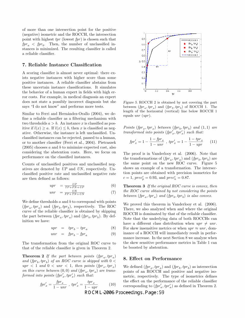
of more than one intersection point for the positive(negative) isometric and the ROCCH, the intersectionpoint with highest tpr (lowest fpr) is chosen such thatfpra < fpr b. Then, the number of unclassified in-stances is minimized. The resulting classifier is calleda reliable classifier.

7. Reliable Instance Classification

A scoring classifier is almost never optimal: there ex-ists negative instances with higher score than somepositive instances. A reliable classifier abstains fromthese uncertain instance classifications. It simulatesthe behavior of a human expert in fields with high er-ror costs. For example, in medical diagnosis an expertdoes not state a possibly incorrect diagnosis but shesays “I do not know” and performs more tests.

Similar to Ferri and Hernandez-Orallo (2004), we de-fine a reliable classifier as a filtering mechanism withtwo thresholds a > b. An instance x is classified as pos-itive if l(x) ≥ a. If l(x) ≤ b, then x is classified as neg-ative. Otherwise, the instance is left unclassified. Un-classified instances can be rejected, passed to a human,or to another classifier (Ferri et al., 2004). Pietraszek(2005) chooses a and b to minimize expected cost, alsoconsidering the abstention costs. Here, we focus onperformance on the classified instances.

Counts of unclassified positives and unclassified neg-atives are denoted by UP and UN , respectively. Un-classified positive rate and unclassified negative rateare then defined as follows:

upr = UPTP+FN+UP (6)

unr = UNFP+TN+UN (7)

We define thresholds a and b to correspond with points(fpra, tpra) and (fpr b, tpr b), respectively. The ROCcurve of the reliable classifier is obtained by skippingthe part between (fpra, tpra) and (fpr b, tpr b). By def-inition we have:

upr = tpr b − tpra (8)unr = fpr b − fpra (9)

The transformation from the original ROC curve tothat of the reliable classifier is given in Theorem 2.

Theorem 2 If the part between points (fpra, tpra)and (fpr b, tpr b) of an ROC curve is skipped with 0 <upr < 1 and 0 < unr < 1, then points (fprx, tprx)on this curve between (0, 0) and (fpra, tpra) are trans-formed into points (fpr ′x, tpr ′x) such that:

fpr ′x =fprx

1− unr, tpr ′x =

tprx

1− upr(10)

Figure 5. ROCCH 2 is obtained by not covering the partbetween (fpra, tpra) and (fprb, tprb) of ROCCH 1. Thelength of the horizontal (vertical) line below ROCCH 1equals unr (upr).

Points (fprx, tprx) between (fpr b, tpr b) and (1, 1) aretransformed into points (fpr ′x, tpr ′x) such that:

fpr ′x = 1− 1− fprx

1− unr, tpr ′x = 1− 1− tprx

1− upr(11)

The proof is in Vanderlooy et al. (2006). Note thatthe transformations of (fpra, tpra) and (fpr b, tpr b) arethe same point on the new ROC curve. Figure 5shows an example of a transformation. The intersec-tion points are obtained with precision isometrics forc = 1, precc

p = 0.93, and preccn = 0.87.

Theorem 3 If the original ROC curve is convex, thenthe ROC curve obtained by not considering the pointsbetween (fpra, tpra) and (fpr b, tpr b) is also convex.

We proved this theorem in Vanderlooy et al. (2006).There, we also analyzed when and where the originalROCCH is dominated by that of the reliable classifier.Note that the underlying data of both ROCCHs canhave a different class distribution when upr 6= unr .For skew insensitive metrics or when upr ≈ unr , dom-inance of a ROCCH will immediately result in perfor-mance increase. In the next Section 8 we analyze whenthe skew sensitive performance metrics in Table 1 canbe boosted by abstention.

8. Effect on Performance

We defined (fpra, tpra) and (fpr b, tpr b) as intersectionpoints of an ROCCH and positive and negative iso-metric, respectively. The type of isometrics definesthe effect on the performance of the reliable classifiercorresponding to (fpr ′a, tpr ′a) as defined in Theorem 2.

8.1. Precision

Theorem 4 provides an easy and computationally effi-cient approach to construct a classifier with a desiredprecision per class.

Theorem 4 If points (fpra, tpra) and (fpr b, tpr b) aredefined by an precc

p-isometric and preccn-isometric re-

spectively, then the point (fpr ′a, tpr ′a) has the precisionsof both isometrics.

The proof of this theorem and also of following the-orems are included in the appendix. Since isometricsof skew sensitive performance metrics are used, theapproach does not commit to costs and class distribu-tions3. Thus, when the application domain changesa new reliable classifier can be constructed from theoriginal ROC curve only.

Theorem 4 together with the next Theorem 5 providesan approach to construct a classifier with desired ac-curacy. This approach overcomes the problems withaccuracy explained in Section 4. From the proof itfollows that if the precisions are not equal, then theaccuracy is bounded by the smallest and largest pre-cision.

Theorem 5 If point (fpr ′a, tpr ′a) has preccp = precc

n,then the accuracy in this point equals the precisions.

8.2. F -measure

Theorem 6 shows that also the F -measure can beboosted on both classes if a part of an ROC curve is notcovered. In this case, the resulting classifier has higherperformance than defined by both isometrics. Figure6 gives an example where positive (negative) perfor-mance is increased with approximately 5% (10%).

Theorem 6 If points (fpra, tpra) and (fpr b, tpr b) aredefined by an F c,α

p -isometric and F c,αn -isometric re-

spectively, then the point (fpr ′a, tpr ′a) has higher per-formance than defined by both isometrics.

8.3. Generalized m-estimate

To analyze the effect of abstention on the gm-estimate,we can consider the number of a priori classified in-stances m to be fixed or the parameter m to be fixed.

Consider the case when m is not changed after trans-formation. In this case upr and unr can change thedistribution of a priori instances over the classes. Ifupr < unr , then the distribution of these instances in

3Remember that, although our proofs use the simplest

case c = NP

, the results are also valid for c = c(p,n)c(n,p)

NP

.

Figure 6. Designing with F -measure isometrics: F 2,1p =

0.72 in (fpra, tpra) and F 2,1n = 0.75 in (fprb, tprb). The

reliable classifier represented by (fpr ′a, tpr ′

a) has F 1.84,1p =

0.7693 and F 1.84,1n = 0.8597. The abstention is represented

by upr = 0.1541 and unr = 0.2116.

the positive gm-estimate moves to the true positivesresulting in higher performance. For the negative gm-estimate, the distribution moves to the false negativesresulting in lower performance. The case of upr > unris the other way around. Therefore, an increase in per-formance in both classes is only possible iff upr = unr .

For the case when m is not changed after transfor-mation, a similar reasoning results in improvement ofthe positive gm-estimate if upr ≤ unr and tpra ≥fpra. The latter condition holds for all points on theROCCH. Similarly, improvement in the negative gm-estimate occurs if upr ≥ unr and tpr b ≥ fpr b. Thus,we find the following theorems for the gm-estimate.

Theorem 7 If point (fpra, tpra) is defined by angmc,m

p -estimate isometric with m > 0 and if upr ≤unr, then the point (fpr ′a, tpr ′a) has at least the posi-tive performance defined by that isometric.

Theorem 8 If point (fpr b, tpr b) is defined by angmc,m

n -estimate isometric with m > 0 and if upr ≥unr, then the point (fpr ′a, tpr ′a) has at least the nega-tive performance defined by that isometric.

Corollary 1 If points (fpra, tpra) and (fpr b, tpr b) aredefined by an gmc,m

p -estimate isometric and gmc,mn -

estimate isometric respectively with m > 0 and ifupr = unr, then the point (fpr ′a, tpr ′a) has at least thegm-estimates of both isometrics.

We suggest to use the gm-estimate for the minorityclass only and to use a normal precision for the ma-jority class. From Theorems 7 and 8, if the minority

Figure 7. Designing with precision and gm-estimate iso-metrics: prec0.3

p = 0.97 in (fpra, tpra) and gm0.3,0.1n =

0.55 in (fprb, tprb). The reliable classifier represented by(fpr ′

a, tpr ′a) has prec0.3

p = 0.97 and gm0.34,0.18n = 0.5584.

The abstention is represented by upr = 0.4549 and unr =0.3763.

class is the positive (negative) class, then we need anabstention characterized by upr ≤ unr (upr ≥ unr).

Figure 7 shows an example with fixed m and the neg-ative class as minority class. Therefore, we want thatthe gmc,m

n -estimate isometric covers a large part inROC space and consequently the condition upr ≥ unris easily satisfied.

9. Conclusions

A reliable classifier abstains from uncertain instanceclassifications. Benefits are significant in applicationdomains with high error costs, e.g., medical diagnosisand legal practice. A classifier is transformed into areliable one by not covering a part of its ROC curve.This part is defined by two isometrics indicating per-formance on a different class.

In case of a classifier and corresponding reliable clas-sifier, dominance of an ROC curve immediately repre-sents an increase in performance if the underlying dataof both curves have approximately equal class distribu-tions. Since this assumption is too strong, we analyzedwhen performance can be boosted by abstention.

We showed how to construct a (reliable) classifier witha desired precision per class. We did the same foraccuracy. For the F -measure a classifier is obtainedwith at least the desired performance per class. Toprevent a possible performance decrease with the gm-estimate, we propose to use it for the minority classand to use a normal precision for the majority class.

We may conclude that the proposed approach is able toboost performance on each class simultaneously. Ben-efits of the approach are numerous: it guarantees aclassifier with an acceptable performance in domainswith high error costs, it is efficient in terms of timeand space, classifier independent, and it incorporateschanging error costs and class distributions easily.

Acknowledgments

We thank the reviewers for useful comments and sug-gestions. This work was partially supported by theDutch Organization for Scientific Research (NWO),grant nr: 634.000.435.

References

Fawcett, T. (2003). ROC graphs: Notes and practi-cal considerations for researchers (Technical ReportHPL-2003-4). HP Laboratories.

Ferri, C., Flach, P., & Hernandez-Orallo, J. (2004).Delegating classifiers. Proceedings of the 1st Inter-national Workshop on ROC Analysis in ArtificialIntelligence (ROCAI-2004) (pp. 37–44).

Ferri, C., & Hernandez-Orallo, J. (2004). Cautiousclassifiers. Proceedings of the 1st InternationalWorkshop on ROC Analysis in Artificial Intelligence(ROCAI-2004) (pp. 27–36).

Flach, P. (2003). The geometry of ROC space: Un-derstanding machine learning metrics through ROCisometrics. Proceedings of the 20th InternationalConference on Machine Learning (ICML-2003) (pp.194–201).

Furnkranz, J., & Flach, P. (2005). Roc ‘n’ rule learn-ing – towards a better understanding of coveringalgorithms. Machine Learning, 58, 39–77.

Lachiche, N., & Flach, P. (2003). Improving accu-racy and cost of two-class and multi-class probabilis-tic classifiers using ROC curves. Proceedings of the20th International Conference on Machine Learning(ICML-2003) (pp. 416–423).

Lavrac, N., & Dzeroski, S. (1994). Inductive logic pro-gramming: Techniques and applications. Ellis Hor-wood, New York.

Pietraszek, T. (2005). Optimizing abstaining classifiersusing ROC analysis. Proceedings of the 22th Inter-national Conference on Machine Learning (ICML-2005) (pp. 665–672).

Provost, F., & Fawcett, T. (2001). Robust classifica-tion for imprecise environments. Machine Learning,42, 203–231.

Provost, F., Fawcett, T., & Kohavi, R. (1998). Thecase against accuracy estimation for comparing in-duction algorithms. Proceedings of the 15th Inter-national Conference on Machine Learning (ICML-1998) (pp. 43–48).

Rijsbergen, C. V. (1979). Information retrieval. De-partment of Computer Science, University of Glas-gow. 2nd edition.

Vanderlooy, S., Sprinkhuizen-Kuyper, I., & Smirnov,E. (2006). Reliable classifiers in ROC space.Proceedings of the 15th Annual Machine Learn-ing Conference of Belgium and the Netherlands(BENELEARN-2006) (pp. 113–120).

A. Proofs

Proof of Theorem 4The positive precisions in (fpra, tpra) and (fpr ′a, tpr ′a)are defined as follows:

preccp (fpra, tpra) =

tpra

tpra + c fpra

(12)

precc′

p

(fpr ′a, tpr ′a

)=

tpr ′atpr ′a + c′ fpr ′a

(13)

with c′ = c 1−unr1−upr . Substitution of Eq. 10 in Eq. 13

results in Eq 12. In a similar way, Eq. 11 is used toshow that the negative precisions in (fpr b, tpr b) and(fpr ′b, tpr

′b) are the same. The theorem follows since

(fpr ′b, tpr′b) = (fpr ′a, tpr ′a).

Proof of Theorem 5Since the positive precision and negative precision in(fpr ′a, tpr ′a) are equal, we can write:

tpr ′a = a(tpr ′a + c′ fpr ′a

)(14)

tnr ′a = a

(tnr ′a +

1c′

fnr ′a

)(15)

with a = precc′

p = precc′

n . It follows that:

tpr ′a + c′ tnr ′a =

a(tpr ′a + c′ fpr ′a + c′ tnr ′a + fnr ′a

)(16)

or equivalently:

a =tpr ′a + c′ tnr ′a

tpr ′a + c′ fpr ′a + c′ tnr ′a + fnr ′a(17)

and this is the accuracy with skew ratio c′.

Proof of Theorem 6The positive F -measures in (fpra, tpra) and(fpr ′a, tpr ′a) are defined as follows:

F c,αp (fpra, tpra) =

(1 + α2

)tpra

α2 + tpra + c fpra

(18)

F c′,αp

(fpr ′a, tpr ′a

)=

(1 + α2

)tpr ′a

α2 + tpr ′a + c′ fpr ′a(19)

Using Eq. 10 and c′ = c 1−unr1−upr , the right-hand side of

Eq. 19 becomes: (1 + α2

)tpra

α2(1− upr) + tpra + c fpra

(20)

It follows that F c′,αp

(fpr ′a, tpr ′a

)> F c,α

p (fpra, tpra)since 0 < upr < 1. The case of the negative F -measureis similar.

Proof of Theorem 7The positive gm-estimates in (fpra, tpra) and(fpr ′a, tpr ′a) are defined as follows:

gmc,mp (fpra, tpra) = tpr+m

tpr+c fpr+m(1+c) (21)

gmc′,m′

p

(fpr ′a, tpr ′a

)= tpr ′+m′

tpr ′+c′ fpr ′+m′(1+c′) (22)

with m = mP+N , and c′ = c 1−unr

1−upr .

Case 1: m is not changed after transformationIn this case we can write m′ = m

P (1−upr)+N(1−unr) .Substitution of Eq. 10 in Eq. 22 results in the follow-ing right-hand side:

tpr + m 1−uprP (1−upr)+N(1−unr)

tpr + c fpr + m(1 + c)(23)

Clearly, gmc′,m′

p

(fpr ′a, tpr ′a

)≥ gmc,m

p (fpra, tpra) iff:

1− upr

P (1− upr) + N(1− unr)≥ 1

P + N(24)

This holds iff upr ≤ unr .

Case 2: m is not changed after transformationSubstitution of Eq. 10 in Eq. 22 with fixed m resultsin the following right-hand side:

tpr + m(1− upr)tpr + c fpr + m(1− upr + c(1− unr))

(25)

Straightforward computation results ingmc′,m

p

(fpr ′a, tpr ′a

)≥ gmc,m

p (fpra, tpra) iff:

m(unr − upr) + (tpra unr − fpra upr) ≥ 0 (26)

This holds if upr ≤ unr and tpra ≥ fpra.

Proof of Theorem 8The proof is similar to that of Theorem 7.

A Comparison of Different ROC Measures for Ordinal Regression

Willem Waegeman Willem.Waegeman@UGent.be

Department of Electrical Energy, Systems and Automation, Ghent University, Technologiepark 913, B-9052Ghent, Belgium

Bernard De Baets Bernard.DeBaets@UGent.be

Department of Applied Mathematics, Biometrics and Process Control, Ghent University, Coupure links 653,B-9000 Ghent, Belgium

Luc Boullart Luc.Boullart@UGent.be

Department of Electrical Energy, Systems and Automation, Ghent University, Technologiepark 913, B-9052Ghent, Belgium

Abstract

Ordinal regression learning has characteris-tics of both multi-class classification and met-ric regression because labels take ordered,discrete values. In applications of ordinal re-gression, the misclassification cost among theclasses often differs and with different mis-classification costs the common performancemeasures are not appropriate. Therefore weextend ROC analysis principles to ordinal re-gression. We derive an exact expression forthe volume under the ROC surface (VUS)spanned by the true positive rates for eachclass and show its interpretation as the prob-ability that a randomly drawn sequence withone object of each class is correctly ranked.Because the computation of V US has a hugetime complexity, we also propose three ap-proximations to this measure. Furthermore,the properties of VUS and its relationshipwith the approximations are analyzed by sim-ulation. The results demonstrate that opti-mizing various measures will lead to differentmodels.

1. Introduction

In multi-class classification labels are picked from aset of unordered categories. In metric regression labelsmight take continuous values. Ordinal regression can

Appearing in Proceedings of the ICML 2006 workshop onROC Analysis in Machine Learning, Pittsburgh, USA,2006. Copyright 2006 by the author(s)/owner(s).

be located in between these learning problems becausehere labels are chosen from a set of ordered categories.Applications of ordinal regression frequently arise indomains where humans are part of the data gener-ation process. When humans assess objects for theirbeauty, quality, suitability or any other characteristic,they really prefer to qualify them with ordinal labelsinstead of continuous scores. This kind of datasets isobtained in information retrieval and quality control,where the user or the human expert frequently evalu-ates objects with linguistic terms, varying from “verybad” to “very good” for example. Also in medicine andsocial sciences, where many datasets originate by in-teraction with humans, ordinal regression models canbe used.

In these applications of ordinal regression one is oftenthe most interested in a subset of the classes. In manycases these classes of interest are the “extreme” cat-egories, such as the documents with the highest rel-evance to the query or the products with the lowestquality. Moreover, there is often an unequal numberof training objects for the different categories in real-world ordinal regression problems. The overall classi-fication rate or mean absolute error are in these casesnot the most pertinent performance measures. Crite-ria such as the area under the receiver operating char-acteristics (ROC) curve — which is related to definingan optimal ranking of the objects — are more appro-priate. This article aims to discuss possible extensionsof ROC analysis for ordinal regression.

Nowadays the area under the ROC curve is used as astandard performance measure in many fields where abinary classification system is needed. A ROC curve iscreated by plotting the true positive rate (TPR) versus

y = −1 y = 1y = −1 TN FP n−y = 1 FN TP n+

NP PP n

Table 1: Confusion matrix for a two class classificationproblem of size n

the false positive rate (FPR). The TPR (or sensitiv-ity) and the FPR (also known as 1 - specificity) arecomputed from the confusion matrix or contingencytable (shown in Table 1). Sensitivity is defined asthe number of positive predicted examples from thepositive class TP divided by the number of positiveexamples n+ and specificity is defined as the numberof negative predicted examples TN from the negativeclass divided by the number of negative examples n−:

Sens = TPR =TP

TP + FN(1)

Spec = TNR = 1− FPR =TN

TN + FP(2)

With a classifier that estimates a continuous functionf , the class prediction y for an object x is obtained bythe following rule:

y = sgn(f(x) + b) (3)

The points defining the ROC curve can then be com-puted by varying the threshold b from the most nega-tive to the most positive function value and the areaunder the ROC curve (AUC) gives an impression ofquality of the classifier. It has been shown [Cortes &Mohri, 2003,Yan et al., 2003] that the AUC is equiv-alent to the Wilcoxon-Mann-Whitney statistic:

WMW = AUC(f) =1

n−n+

n−∑i=1

n+∑j=1

If(xi)<f(xj) (4)

The value of the indicator function I will be one whenits argument is true and zero otherwise. The mea-sure AUC(f) can be seen as a nonparametric estimatefor the probability that the function value of an ob-ject randomly drawn from the negative class is strictlysmaller than the function value of an object randomlydrawn from the positive class:

AUC(f) = P (f(xi) < f(xj) | yi = −1 ∧ yj = 1)) (5)

2. ROC Measures for OrdinalRegression

Recently, different approaches have been proposed toextend ROC analysis for multi-class classification. In

the most general case, the volume under the ROC sur-face (V US) has to be minimized in multi-class clas-sification. The ROC surface can be seen as a Paretofront, where each objective corresponds to one dimen-sion. In case there are more then two classes (let’ssay r), then the number of objectives depends on themulti-class method that is used:

• For a one-versus-all method, r functions fk areestimated that try to separate objects of class kfrom the other classes. As a consequence mis-classification costs for each class are fixed and thecorresponding ROC surface will have r dimensionsrepresenting the true positive rates TPRk for eachclass [Flach, 2004]. ROC points are here obtainedby varying the thresholds bk in the prediction ruley = argmaxkfk(x) + bk.

• For a one-versus-one method, a function fkl is es-timated for each pair of classes, which allows tospecify the cost for a misclassification of an objectof class k predicted as class l. The correspondingROC space is in this case spanned by r(r−1)

2 objec-tives [Ferri et al., 2003]. A prediction for new in-stances is done by majority voting over all r(r−1)

2classifiers based on the outcomes sgn(fkl + bkl).

In ordinal regression the picture is slightly differ-ent. The vast majority of existing methods for or-dinal regression — including traditional statisticalmethods like cumulative logit models and their vari-ants [Agresti, 2002], kernel methods [Chu & Keerthi,2005,Shashua & Levin, 2003] and bayesian approaches[Chu & Gharhamani, 2005] — fit in general one func-tion f to the data together with r − 1 thresholds bk

for r ordered classes. New observations can then beclassified by predicting them into the class k for whichit holds that

bk−1 < f(x) ≤ bk with b0 = −∞ and br = +∞. (6)

The simplicity of this kind of models has as disadvan-tage that one can not control the cost of misclassifyingan object of a given class into another specified class.In other words, like in one-versus-all multi-class clas-sification only r objectives can be simultaneously min-imized. Therefore one could wonder whether a one-versus-one approach could be useful for ordinal regres-sion. However, the answer is negative because it wouldlead to a more complex model with more variables tobe estimated. Fortunately, Misclassification costs arealways proportional to the absolute difference betweenthe real and the predicted class, so defining a loss func-tion with this property will solve the problem [Rennie& Srebro, 2005].

We will further assume that the misclassification costsare fixed for each class (they are always to proportionalto the absolute difference between the real and the pre-dicted label). Like in binary classification, we want amodel f that imposes an optimal ranking of the dataobjects. There are several ways to define an optimalranking. By analogy with (5) an optimal ranking couldhere be defined as a ranking that maximizes the jointprobability that an r-tuple (x1, ..., xr) is correctly or-dered where each element xk is randomly drawn fromclass k. This probability is given by

P (r−1∧k=1

(f(xk) < f(xk+1) | yk = k) (7)

and it can be estimated for a given model by count-ing the number of ordered r-tuples occurring in thetraining dataset, i.e.

OrdTuples(f) =1Qr

k=1 nk

X

yj1<...<yjr

If(xj1 )<...<f(xjr ) (8)

Here nk stands for the number of objects with label k.It is straightforward to see that OrdTuples(f) reducesto (4) in case of two classes. Furthermore, we can showthe following.

Theorem 2.1 Given a continuous function f that im-poses a ranking over a dataset with r ordered classes,OrdTuples(f) is the volume under the ROC surface(V USord(f)) spanned by the true positive rates foreach class.

In statistics there has some related work on this topic.[Dreisetl et al., 2000] derive formulas for the varianceof V USord and the covariance between two volumesin the three class case. This work is extended to thegeneral r-class case in [Nakas & Yiannoutsos, 2004].They conclude that bootstrapping is preferred over U-statistics for large values of n and r. In this article wefocus more on the use of V USord(f) as performancemeasure for ordinal regression problems.

For three ordered classes the ROC surface can be vi-sualized. We have constructed this ROC surface for asynthetic dataset. We sampled 3 ∗ 100 instances from3 bivariate Gaussian clusters with consecutive ranks.The mean of the clusters was set to (10,10), (20,10)and (20,20) respectively, σ1 and σ2 were set to 5 forthe first two clusters and were set to 7 for the lastcluster. ρ was fixed to 0. This dataset is visualized inFigure 1. We used the support vector ordinal regres-sion algorithm of [Chu & Keerthi, 2005] to estimate

Figure 1: Synthetic dataset

Figure 2: 3D ROC surface for the synthetic dataset

the function f , without looking at the thresholds. TheROC surface is shown in Figure 2.

Optimizing the AUC instead of accuracy has beensuggested for binary classification, for example withgradient descent or a quadratic solver. However, thecomputation of V USord(f) has a large time complex-ity. The function I is evaluated

∏rk=1 nk times, which

is exponential in the number of classes r. As a con-sequence, minimizing V USord(f) will lead to a hardoptimization problem.

We will look at approximations of V USord(f) whichcan be more easily transformed into a suitable lossfunction. The biggest problem is that all r − tuplesneed to be verified. Much would be gained if onlypairs of function values have to be correctly ranked ineach evaluation of I. This is another way of evaluatingthe imposed ranking. We discuss here three approx-imations of V USord that all reduce to I-evaluations

(a) First ROC-curve

(b) Second ROC-curve

Figure 3: The three dimensional ROC surface approx-imated by a set of two ROC-curves for the syntheticdataset.

with only one condition.

The first approximation Cons(f) is directly deducedfrom the way the majority of existing ordinal regres-sion models are constructed. With a function f andr− 1 thresholds one could look at threshold bk as pro-viding the separation between the consecutive ranks kand k + 1. Varying this threshold will change the pro-portion between objects predicted lower than or equalto class k and objects predicted higher than class k.This corresponds to measuring the non-weighted sumof r− 1 two-dimensional ROC curves representing thetrade-off between consecutive classes:

Cons(f) =1

r − 1

r−1X

l=1

AUCl(f) (9)

AUCl(f) =1

Pli=1 ni

Pnj=l+1 nj

X

i:yi≤l

X

j:yj>l

If(xi)<f(xj)

The two ROC curves belonging to the syntheticdataset are shown in figure 3.

For a second approximation of V USord(f) we lookedat the statistical literature. In nonparametric statis-

tics the Jonckheere-Terpstra test is known as a morepowerful alternative for a Kruskal-Wallis test for test-ing

H0 : µ1 ≤ µ2 ≤ ... ≤ µr (10)

versus the one side alternative

Ha : µ1 ≥ µ2 ≥ ... ≥ µr (11)

if there is a cdf F for which Fk(x) = F (x− µk)). It iscomposed of a set of one sided WMW-tests:

JT =∑i<j

WMWij (12)

JT computes the WMW statistic for all possible pairsof classes, which is the same as computing the AUC foreach pair of classes. This has been done for one-versus-one multi-class classification [Hand & Till, 2001],which gives rise to the following approximation:

Ovo(f) =2

r(r − 1)

∑l<k

AUClk(f) (13)

AUClk(f) =1

nlnk

∑i:yi=l

∑j:yj=k

If(xi)<f(xj)

A third measure could exist of counting the numberpairs that are correctly ranked among all possible pairsof data objects:

Pairs(f) =1∑

k<l nknl

n∑i=1

n∑j=1;yi<yj

If(xi)<f(xj)(14)

A loss function based on (14) is used in the ordinalregression method of [Herbrich et al., 2000]. The dif-ference with Ovo(f) is that here a weighted average ofthe ROC areas for each of pair of classes is taken. Theweights are the prior πk probabilities of observing anobject of class k, i.e.

Pairs(f) =2

r(r − 1)

∑l<k

πkπlAUClk(f) (15)

3. Simulation experiments

To see the characteristics of the different measures, weconducted some simulation experiments. In the firstexperiment we wanted to find out which values are ob-tained for different levels of separability and for an in-creasing number of classes. Therefore we assume thatthe function values of the model f can be representedby a distribution with cdf F (x), in which the functionvalues for the objects of class k are distributed with cdfFk(x) = F (x − kd). Furthermore we chose to sample

Figure 4: Relation between V USord(f) and Cons(f)for r = 1, ..., 5 and d = 0, ..., 5 with step size 0.25. Thevalues are averaged over 20 runs.

Figure 5: Relation between V USord(f) and Ovo(f)for r = 1, ..., 5 and d = 0, ..., 5 with step size 0.25. Thevalues are averaged over 20 runs.

from a Gaussian distribution with standard deviationσ = 1. So the function values conditioned on the la-bels are normally distributed with equidistant orderedmeans. Repeatedly 100 data points were sampled fromeach class while we increased the distance d betweenthe means of consecutive clusters. We started at d = 0(random classifier) and stopped at d = 5 (as good asperfect separation) with step size 0.25.

The results obtained for V USord(f), Cons(f) andOvo(f) are graphically compared. In this simulationall classes have the same prior of occurring, so Ovo(f)and Pairs(f) will always have the same value. Conse-quently the results for Pairs(f) are omitted. The rela-tionship between V USord(f) and Cons(f) on the oneside and between V USord(f) and Ovo(f) on the otherside are shown in Figures 4 and 5. One can see that,as expected, the relation between V USord(f) and theother two measures is without doubt nonlinear. Theexpected value for V USord(f) heavily depends on thenumber of classes, while this is not the case for theapproximations. The approximations all take an aver-age over a set of two dimensional ROC-curves, so theirexpected value is never lower than a half, irrespective

Figure 6: Relation between Cons(f) and Pairs(f) forr = 1, ..., 5 and d = 0, ..., 5 with step size 0.25. Thevalues are averaged over 20 runs.

of the number of classes. Nevertheless, one can alsosee that V USord(f) converges rapidly to one when thedistance between the subsequent means increases. Inaddition, Cons(f) and Ovo(f) behave quite similarin this simulation. This is also shown in Figure 6.Their observed values become more dissimilar whenthe number of classes increases.

In a second experiment we wanted to investigatewhether optimizing the various performance measureswould lead to the same model. For two measures M1

and M2 this implies that

∀f, f∗ ∈ H : M1(f) < M1(f∗) ⇔ M2(f) < M2(f∗)(16)∀f, f∗ ∈ H : M1(f) = M1(f∗) ⇔ M2(f) = M2(f∗).(17)

The following experiment was set up to test whetherthis property holds for the four measures. All measuresonly quantify the quality of the ordering of a datasetfor a function f . For a dataset of size n there are n!possible rankings of the objects, so evaluating them allis computationally intractable. Therefore we sampledrandomly 1000 rankings from all possible orderings ofthe dataset. We assumed we had 50 samples per classwith four ordered classes, resulting in a sample size of200 objects and 200! possible rankings. The resultsare given in Figure 7, which shows the distributionsof all measures together with pairwise scatter plots.All classes again have the same prior of occurring,so Ovo(f) and Pairs(f) have a perfect correlation.This is however not true for the other measures. Onecan clearly see that for no pair of measures conditions(16) or (17) hold. In general, V USord(f), Cons(f) andOvo(f) will have different maxima over a hypothesisspace H and a given dataset. So, optimizing one of theproposed approximations of V USord(f) will give riseto different classifiers.

Figure 7: Histograms and pairwise scatter plots for all the measures.

4. Discussion and further research

In this article we argued that accuracy or mean ab-solute error are not the most powerful performancemeasures to evaluate ordinal regression models whenmisclassification costs are not equal for each class orwhen the data is unbalanced. Therefore we proposedsome new measures, which extend binary and multi-class ROC analysis to ordinal regression. They allmeasure the quality of the ranking imposed by an or-dinal regression model. First of all we showed thatcounting the number of ordered r-tuples in the rank-ing is equivalent to the area under the r-dimensionalROC curve spanned by the true positive rates of allclasses. However, V USord(f) can’t be transformedeasily into a suitable loss function for learning algo-rithms, so three approximations were also analyzed.By simulation we showed that these four measures ingeneral have a different distribution and that none ofthem is a monotone function of another. Further re-search will be devoted to converting measures like thearea under the ROC curve into a loss function for alearning algorithm and to further analyse the charac-teristics of the presented measures.

Acknowledgments

The authors would like to thank Bruno Bauwens foruseful discussions. Willem Waegeman is supported bya grant of the “Institute for the Promotion of Inno-vation through Science and Technology in Flanders(IWT-Vlaanderen)”.

References

Agresti, A. (2002). Categorical Data Analysis, 2ndversion. John Wiley and Suns Publications.

Chu, W., & Gharhamani, Z. (2005). Gaussianprocesses for ordinal regression. Journal of MachineLearning Research, 6, 1019–1041.

Chu, W., & Keerthi, S. (2005). New approaches tosupport vector ordinal regression. Proceedings ofthe International Conference on Machine Learning,Bonn, Germany (pp. 321–328).

Cortes, C., & Mohri, M. (2003). AUC optimiza-tion versus error rate minimization. In Advances inNeural Information Processing Systems, Vancouver,Canada. The MIT Press.

Dreisetl, S., Ohno-Machado, L., & Binder, M. (2000).

Comparing three-class diagnostic tests by three-wayroc analysis. Medical Decision Making, 20, 323–331.

Ferri, C., Hernandez-Orallo, J., & Salido, M. (2003).Volume under ROC surface for multi-class problems.In Proceedings of the European Conference on Ma-chine Learning, Dubrovnik, Croatia (pp. 108–120).

Flach, P. (2004). The many faces of ROC analysisin machine learning. Tutorial presented at the Eu-ropean Conference on Machine Learning, Valencia,Spain.

Hand, D. J., & Till, R. J. (2001). A simple generaliza-tion of the area under the ROC curve for multipleclass problems. Machine Learning, 45, 171–186.

Herbrich, R., Graepel, T., & Obermayer, K. (2000).Large margin rank boundaries for ordinal regression.Advances in Large Margin Classifiers (pp. 115–132).The MIT Press.

Nakas, C. T., & Yiannoutsos, C. T. (2004). Orderedmultiple-class roc analysis with continuous measure-ments. Statistics in Medicine, 22, 3437–3449.

Rennie, J. D. M., & Srebro, N. (2005). Loss func-tions for preference levels: Regression with discrete,ordered labels. Proceedings of the IJCAI Multidisci-plinary Workshop on Advances in Preference Han-dling, Edinburgh, Scotland (pp. 180–186).

Shashua, A., & Levin, A. (2003). Ranking with largemargin principle: Two approaches. Proceedings ofthe International Conference on Neural InformationProcessing Systems, Vancouver, Canada (pp. 937–944). Cambridge MA: MIT Press.

Yan, L., Dodier, R., Mozer, M. C., & Wolniewiecz,R. (2003). Optimizing classifier performance via anapproximation to the Wilcoxon-Mann-Whitney sta-tistic. Proceedings of the International Conferenceon Machine Learning, Washington D. C., USA (pp.848–855).

Upper and Lower Bounds of Area Under ROC Curves and Index ofDiscriminability of Classifier Performance

Shane T. Mueller stmuelle@indiana.edu

Indiana University, Department of Psychological and Brain Sciences, 1101 East 10th Street, Bloomington, IN47404

Jun Zhang junz@umich.edu

University of Michigan, Department of Psychology, 530 Church Street Ann Arbor, MI 48109-1043

Abstract

Area under an ROC curve plays an impor-tant role in estimating discrimination per-formance – a well-known theorem by Green(1964) states that ROC area equals the per-centage of correct in two-alternative forced-choice setting. When only single data point isavailable, the upper and lower bound of dis-crimination performance can be constructedbased on the maximum and minimum areaof legitimate ROC curves constrained to passthrough that data point. This position paper,after reviewing a property of ROC curves pa-rameterized by the likelihood-ratio, presentsour recently derived formula of estimatingsuch bounds (Zhang & Mueller, 2005).

1. Introduction

Signal detection theory (Green & Swets, 1966) is com-monly used to interpret data from tasks in which stim-uli (e.g., tones, medical images, emails) are presentedto an operator (experimenter, medical examiner, clas-sification algorithm), who must determine which oneof two categories (high or low, malignant or benign,junk or real) the stimulus belongs in. These tasksyield a pair of measures of behavioral performance:the Hit Rate (H), also called “true positive” rate, andthe False Alarm Rate (F ), also called “false positive”rate. (The other two rates, those of Miss or “falsenegative” and of Correct Rejection or “true negative”,are simply one minus H and F , respectively.) H andF are typically transformed into indices of sensitivity

Appearing in Proceedings of the ICML 2006 workshop onROC Analysis in Machine Learning, Pittsburgh, USA,2006. Copyright 2006 by the author(s)/owner(s).

and bias based on assumptions about an underlyingstatistical model. A curve c 7→ (F (c),H(c)) in theROC (Receiver-Operating Characteristic) space is acollection of hit and false-alarm rates while the opera-tor/receiver modifies the cutoff criterion c of acceptingthe input stimulus as belonging to one category versusanother; often c is the likelihood ratio of the evidencefavoring the two corresponding hypotheses, or a mono-tonic transformation thereof. In the machine learningcontext, we map the “operator/receiver” in the SDTsense to a “classification algorithm” or simply an “al-gorithm”, the “stimulus” as an “input instance” orsimply “instance” which carries one of the two classlabels, and view c as a parameter of the algorithmwhich biases the output of the algorithm to favor onecategory or the other; the optimal setting of c is relatedto the cost structure, i.e., individual payoffs related tocorrect and incorrect classifications.

A well-known result in SDT is Green’s Theorem, whichrelates the discrimination accuracy performance of anoperator to the area under the operator’s (i.e., the clas-sification algorithm’s) ROC curve. This so-called ROCarea is thus a compact measure of how discriminable aclassification algorithm is between binary-class inputs.Consequently, the performance of different algorithmscan be compared by comparing their respective ROCareas.

Often, algorithms reported in the literature may notcontain a tradeoff analysis of the Hit and False Alarmrates produced by varying parameters correspondingto the algorithm’s bias. In these cases, the entire ROCcurve of an algorithm may not be available — in somecases, only a few or even a single point (called “datapoint”) in the ROC space is available. In this case, per-formance comparison across different algorithms be-comes a question of comparing areas of possible ROCcurves constrained to pass through these limited data

points.

In the mathematical psychology community, the prob-lem of estimating area of ROC curves constrained topass through a single data point is particularly wellstudied (Norman, 1964; Pollack & Norman, 1964; Pol-lack & Hsieh, 1969; Grier, 1971; Smith, 1995; Zhang& Mueller, 2005). These estimates of the ROC areado not assume the ROC curves to arise from any spe-cific class of parametric models, and so these estimatesare often referred to as a “non-parametric” indicesof an operator’s discriminability (sensitivity).1 Typ-ically, the upper and lower bounds of discriminabil-ity were obtained by considering the maximal andminimum ROC areas among the class of “admissible”ROC curves satisfying the data constraint. Interest-ingly, though the basic idea was very simple and ad-vanced over 40 years ago (Pollack & Norman, 1964),the popular formula to calculate this index (Grier,1971), dubbed A′ in psychometrics and cognitive psy-chology literature, turned out to be erroneous, at leastinsofar as its commonly understood meaning is con-cerned; moreover, its purported correction (Smith,1995), dubbed A′′, also contained an error. These for-mulae incorrectly calculated the upper bound of ad-missible ROC curves, using either an ROC curve thatwas not admissible (Pollack & Norman, 1964), or onethat was not the maximum for some points (Smith,1995). Zhang and Mueller (2005) rectified the errorand gave the definite answer to the question of non-parametric index of discriminability based on ROC ar-eas.

In this note, we first review the notion of“proper” (or “admissible”) ROC curves and provea lemma basically stating that all ROC curves areproper/admissible when the likelihood functions (forthe two hypotheses) used to construct the ROC curveare parameterized by the likelihood ratio (of those hy-potheses). We then review Green’s Theorem, whichrelated area under an ROC curve to percentage cor-rect in a two-alternative discrimination task. Finally,we present the upper and lower bounds on a 1-pointconstrained ROC area and reproduce some of the basicarguments underlying their derivation. All technicalcontents were taken from Zhang and Mueller (2005).

1Though no parametric assumption is invoked in thederivation of these indices, the solution itself may cor-respond to certain models of underlying likelihood pro-cess, see MacMillan and Creelman, 1996. In other words,parameter-free here does not imply model-free.

2. Slope of ROC curve and likelihoodratio

Recall that, in the traditional signal detection frame-work, an ROC curve uc 7→ (F (uc),H(uc)) is parame-terized by the cutoff criteria value uc along the mea-surement (evidence) axis based on which categoriza-tion decision is made. Given underlying signal distri-bution fs(u) and noise distribution fn(u) of measure-ment value u2, a criterion-based decision rule, whichdictates a “Yes” decision if u > uc and a “No” decisionif u < uc, will give rise to

H(uc) = Pr(Yes|s) = Pr(u > uc|s) =∫ ∞

uc

fs(u)du,

F (uc) = Pr(No|s) = Pr(u > uc|n) =∫ ∞

uc

fn(u)du.

(1)

As uc varies, so do H and F ; they trace out the ROCcurve. Its slope is

dH

dF

∣∣∣∣F=F (uc),H=H(uc)

=H ′(uc)F ′(uc)

=fs(uc)fn(uc)

≡ l(uc) .

With an abuse of notation, we simply write

dH(u)dF (u)

= l(u) . (2)

Note that in the basic setup, the likelihood ratio l(u)as a function of decision criterion u (whose optimalsetting depends on the prior odds and the payoff struc-ture) need not be monotonic. Hence, the ROC curveu 7→ (F (u),H(u)) need not be concave. We now in-troduce the notion of “proper (or admissible) ROCcurves”.

Definition 2.1. A proper (or admissible) ROC curveis a piece-wise continuous curve defined on the unitsquare [0, 1] × [0, 1] connecting the end points (0,0)and (1,1) with non-increasing slope.

The shape of a proper ROC curve is necessarily con-cave (downward-bending) connecting (0,0) and (1,1).It necessarily lies above the line H = F . Next we pro-vide a sufficient and necessary condition for an ROCcurve to be proper/admissible, that is, a concave func-tion bending downward.

Lemma 2.2. An ROC curve is proper if and only ifthe likelihood ratio l(u) is a non-decreasing functionof decision criterion u.

2In machine learning applications, “signal” and “noise”simply refer the two category classes of inputs, and “signaldistribution” and “noise distribution” are likelihood func-tions of the two classes.

Proof. Differentiate both sides of (2) with respect to u

dF

du· d

dF

(dH

dF

)=

dl

du.

Since, according to (1)

dF

du= −fn(u) < 0,

therefore

dl

du≥ 0 ⇐⇒ d

dF

(dH

dF

)≤ 0

indicating that the slope of ROC curve is non-increasing, i.e., the ROC curve is proper.

Now it is well known (see Green & Swets, 1966) thata monotone transformation of measurement axis u 7→v = g(u) does not change the shape of the ROC curve(since it is just a re-parameterization of the curve),so a proper ROC curve will remain proper after anymonotone transformation. On the other hand, whenl(u) is not monotonic, one wonders whether there al-ways exists a parameterization of any ROC curve toturn it into a proper one. Proposition 1 below showsthat the answer is positive — the parameterization ofthe two likelihood functions is to use the likelihoodratio itself!

Proposition 2.3. (Slope monotonicity of ROCcurves parameterized by likelihood-ratio). The slopeof an ROC curve generated from a pair of likelihoodfunctions (F (lc),H(lc)), when parameterized by thelikelihood-ratio lc as the decision criterion, equals thelikelihood-ratio value at each criterion point lc

dH(lc)dF (lc)

= lc. (3)

Proof. When likelihood-ratio lc is used the decisioncutoff criterion, the corresponding hit rate (H) andfalse-alarm rate (F ) are

H(lc) =∫u:l(u)>lc

fs(u)du,

F (lc) =∫u:l(u)>lc

fn(u)du.

Note that here u is to be understood as (in general)a multi-dimensional vector, and du should be under-stood accordingly. Writing out H(lc + δl) − H(lc) ≡δH(lc) explicitly,

δH(lc) =∫u:l(u)>lc+δl

fs(u)du−∫u:l(u)>lc

fs(u)du

= −∫u:lc<l(u)<lc+δl

fs(u)du ' −∫u:l(u)=lc

fs(u) δu

where the last integral∫

δu is carried out on the set∂ ≡ u : l(u) = lc, i.e., across all u’s that satisfyl(u) = lc with given lc. Similarly,

δF (lc) ' −∫u:l(u)=lc

fn(u) δu .

Now, for all u ∈ ∂

fs(u)fn(u)

= l(u) = lc

is constant, from an elementary theorem on ra-tios, which says that if ai/bi = c for i ∈ I(where c is a constant and I is an index set), then(∑

i∈I ai)/(∑

i∈I bi) = c,

δH(lc)δF (lc)

=

∫∂

fs(u) δu∫∂

fn(u) δu=

fs(u) δu

fn(u) δu

∣∣∣∣u∈∂

= lc .

Taking the limit δl → 0 yields (3). .

Proposition 2.3 shows that the slope of ROC curve isalways equal the likelihood-ratio value regardless howit is parameterized, i.e., whether the likelihood-ratiois monotonically or non-monotonically related to theevidence u and whether u is uni- or multi-dimensional.The ROC curve is a signature of a criterion-based de-cision rule, as captured succinctly by the expression

dH(l)dF (l)

= l .

Since H(l) and F (l) give the proportion of hits andfalse alarms when a decision-maker says “Yes” when-ever the likelihood-ratio (of the data) exceeds l, thenδH = H(l + δl) − H(l), δF = F (l + δl) − F (l) arethe amount of hits and false-alarms if he says “Yes”only when the likelihood-ratio falls within the interval(l, l+δl). Their ratio is of course simply the likelihood-ratio.

Under the likelihood-ratio parameterization, the signaldistribution fs(l) = −dH/dl and the noise distributionfn(l) = −dF/dl can be shown to satisfy

Esl =∫ l=∞

l=0

lfs(l)dl ≥ 1 =∫ l=∞

l=0

lfn(l)dl = Enl.

The shape of the ROC curve is determined by H(l) orF (l). In fact, its curvature is

κ =d

dl

(dH

dF

)/

(1 +

(dH

dF

)2)

=1

1 + l2.

3. Green’s Theorem and area underROC curves

The above sections studies the likelihood-ratio classi-fier in a single-instance paradigm — upon receiving aninput instance, the likelihood functions in favor of eachhypothesis are evaluated and compared with a pre-setcriterion to yield a decision of class label. Both priorodds and payoff structure can affect the optimal set-ting of likelihood ratio criterion lc by which class la-bel is assigned. On the other hand, in two-alternativeforce choice paradigms with two two instances, eachinstance is drawn from one category, and the opera-tor must match them to their proper categories. Forexample, an auditory signal may be present in oneof two temporal intervals, and the operator must de-termine which interval contains the signal and whichcontains noise. In this case, the likelihood-ratio clas-sifier, after computing the likelihood-ratios for each ofthe instances, simply compares the two likelihood-ratiovalues la and lb, and matches them to the two class la-bels based on whether la < lb or la > lb. It turnsout that the performance of the likelihood-ratio clas-sifier under the single-instance paradigm (“detectionparadigm”) and under the two-instance forced-choiceparadigm (“identification paradigm”) are related by atheorem first proven by Green (1964).

Proposition 3.1. (Green, 1964). Under thelikelihood-ratio classifier, the area under an ROC curvein a single-observation classification paradigm is equalto the overall probability correct in the two-alternativeforce choice paradigm.

Proof. Following the decision rule of the likelihood-ratio classifier, the percentage of correctly (“PC”)matching the two input instances to the two categoriesis

PC =∫ ∫

0≤lb≤la≤∞fs(la) fn(lb) dla dlb

=∫ ∞

0

(∫ ∞

lb

fs(la) dla

)fn(lb) dlb

=∫ lb=∞

lb=0

H(lb) dF (lb) =∫ F=1

F=0

HdF,

which is the area under the ROC curve lc 7→(F (lc),H(lc)).

Green’s Theorem (Proposition 3.1) motivates one touse the area under an ROC curve to as a mea-sure of discriminability performance of the operator.When multiple pairs of hit and false alarm rates(Fi,Hi)i=1,2,··· (with F1 < F2 < · · · ,H1 < H2 < · · ·)are available, all from the same operator but under ma-nipulation of prior odds and/or payoff structure and

Figure 1. Proper ROC curves through point p must liewithin or on the boundaries of the light shaded regions A1

and A2. The minimum-area proper ROC curve through plies on the boundary of region I.

0 10

1

Hit

Rat

e

False Alarm Rate

(F, H) = p

IA2

A1

with the constraints

0 ≤ · · · ≤ H3 −H2

F3 − F2≤ H2 −H1

F2 − F1≤ ∞,

then it is possible to construct proper ROC curvespassing through these points, and the bounds for theirarea can be constructed. The question of finding theareal bounds of ROC curves passing through a singledata point has received special attention in the past(since Norman, 1964), because as more data pointsare added, the uncertain in ROC area (difference be-tween the upper and lower bounds of area measure) de-creases. We discuss the bounds of 1-point constrainedROC area in the next sections.

4. ROC curves constrained to passthrough a data point

When the data point p = (F,H) is fixed, the non-increasing property of the slope (Corollary 1) imme-diately leads to the conclusion that all proper ROCcurves must fall within or on the bounds of lightshaded regions A1 and A2 (shown in Figure 1). Thisobservation was first made in Norman (1964). Theproper ROC curve with the smallest area lies on theboundary between I and A1 (to the right of p) and A2

(to the left of p), whereas the proper ROC curve withthe largest area lies within or on the boundaries of A1

and A2.

Pollack and Norman (1964) proposed to use the aver-age of the areas A1 + I and A2 + I as an index of dis-criminability (so-called A′), which turns out to equal

Figure 2. Example of a proper ROC curve through p. TheROC curve C, a piecewise linear curve denoted by the darkoutline, is formed by following a path from (0, 0) to (0, 1−y)to (x, 1) (along a straight line that passes through p =(F, H)) and on to (1, 1).

0 10

1

Hit

Rat

e

False Alarm Rate

p = (F, H)

x

y F1 − H

t1

t2

(0, 1 − y)

(x, 1)

1/2+ (H −F )(1+H −F )/(4H(1−F )) (Grier, 1971).However, the A′ index was later mistakenly believed torepresent the average of the maximal and minimum ar-eas of proper ROC curves constrained to pass throughp = (F,H). Rewriting

12((A1 + I) + (A2 + I)) =

12(I + (A1 + A2 + I)),

the mis-conceptualization probably arose from (incor-rectly) taking the area A1 + A2 + I to be the maximalarea of 1-point constrained proper ROC curves while(correcting) taking the are I to be the minimal area ofsuch ROC curves, see Figure 1. It was Smith (1995)who first pointed out this long, but mistakenly-heldbelief, and proceeded to derive the true upper bound(maximal area) of proper ROC curves, to be denotedA+. Smith claimed that, depending on whether p is tothe left or right of the negative diagonal H + F = 1,A+ is the larger of I + A1 and I + A2. This conclu-sion, unfortunately, is still erroneous when p is in theupper left quadrant of ROC space (i.e., F < .5 andH > .5) — in this region, neither I + A1 nor I + A2

represents the upper bound of all proper ROC curvespassing through p.

5. Lower and upper bound of area of1-point constrained proper ROCcurves

The lower bound A− of the area of all proper ROCcurves constrained to pass through a given point p =

(F,H) can be derived easily (the area labelled as I inFigure 1):

A− =12(1 + H − F ).

In Zhang and Mueller (2005), the expression was de-rived for the upper bound A+ of such ROC area.

Proposition 5.1. (Upper Bound of ROC Area). Theareal upper bound A+ of proper ROC curves con-strained to pass through one data point p = (F,H)is

A+ =

1− 2H(1− F ) if F < 0.5 < H ,

1−F2H if F < H < 0.5 ,

1− 1−H2(1−F ) if 0.5 < F < H .

Proof. See Zhang and Mueller (2005).

The ROC curve achieving the maximal area generallyconsists of three segments (as depicted in Figure 2),with the data point p bisecting the middle segment –in other words, t1 = t2 in Figure 2. When p falls inthe F < H < 0.5 (0.5 < F < H, resp) region, then thevertical (horizontal, resp) segment of the maximal-areaROC curve degenerates to the end point (0, 0) ((1, 1),resp), corresponding to y = 1 (x = 1, resp) in Figure 2.

With the upper and lower bounds on ROC area de-rived, Figure 3 plots the difference between thesebounds — that is, the uncertainty in the area of properROC curves that can pass through each point. The fig-ure shows that the smallest differences occur along thepositive and negative diagonals of ROC space, espe-cially for points close to (0, 1) and (.5, .5). The pointswhere there is the greatest difference between the lowerand upper bounds of ROC area are near the linesH = 0 and F = 1. Thus, data observed near theseedges of ROC space can be passed through by properROC curves with a large variability of underlying ar-eas. Consequently, care should be taken when tryingto infer the ROC curve of the observer/algorithm whenthe only known data point regarding its performance(under a single parameter setting) falls within this re-gion.

By averaging the upper and lower bound A = (A+ +A−)/2, we can derive the (non-parametric) index ofdiscriminability performance

A =

34 + H−F

4 − F (1−H) if F ≤ 0.5 ≤ H ;

34 + H−F

4 − F4H if F < H < 0.5 ;

34 + H−F

4 − 1−H4(1−F ) if 0.5 < F < H .

One way to examine A is to plot the “iso-discriminability” curve, i.e, the combinations of F and

Figure 3. Difference between the lower and upper boundsof area of proper ROC curves through every point in ROCspace. Lighter regions indicate smaller differences.

0 10

1

Hit

Rat

e

False Alarm Rate

.00

.05

.10

.15

.20

.25

.30

.35

.40

.45

.50

Figure 4. Iso-discriminability contours in ROC space.Each line corresponds to combinations of F and H thatproduce equal values of A, in increments of 0.05.

0 10

1 A

Hit

Rat

e

False Alarm Rate

H will produce a given value of A. The topography ofA in ROC space can be mapped by drawing isoplethsfor its different constant values. Figure 4 shows thesetopographic maps for A.

Finally, since the slope of any proper ROC curve isrelated to the likelihood ratio of the underlying dis-tributions, we can construct an index of decision bias(Zhang & Mueller, 2005), denoted b, as being orthog-onal to the slope of the constant-A curve (called b):

b =

5−4H1+4F if F ≤ 0.5 ≤ H ;

H2+HH2+F if F < H < 0.5 ;

(1−F )2+1−H(1−F )2+1−F if 0.5 < F < H .

6. Conclusion

We showed that the relationship of ROC slope tolikelihood-ratio is a fundamental relation in ROC anal-ysis, as it is invariant with respect to any contin-uous reparameterization of the stimulus, includingnon-monotonic mapping of uni-dimensional and multi-dimensional evidence in general. We provided an up-per bound for the area of proper ROC curves passingthrough a data point and, together with the knownlower bound, a non-parametric estimate of discrim-inability as defined by the average of maximal andminimum ROC areas.

References

Green, D. M. (1964). General prediction relating yes-no and forced-choice results. Journal of the Acous-tical Society of America, A, 36, 1024.

Green, D. M., & Swets, J. A. (1964). Signal detectiontheory and psychophysics. New York: John Wiley &Sons.

Grier, J. B. (1971). Nonparametric indexes for sensi-tivity and bias: computing formulas. PsychologicalBulletin, 75, 424–429.

Macmillan, N. A., & Creelman, C. D. (1996). Tri-angles in roc space: History and theory of “non-parametric” measures of sensitivity and responsebias. Psychonomic Bulletin & Review, 3, 164–170.

Norman, D. A. (1964). A comparison of data obtainedwith different false-alarm rates. Psychological Re-view, 71, 243–246.

Peterson, W. W., Birdsall, T. G., & Fox, W. C. (1954).The theory of signal detectability. Transactions ofthe IRE Professional Group on Information Theory(pp. 171–212).

Pollack, I., & Hsieh, R. (1969). Sampling variabilityof the area under roc curve and d′e. PsychologicalBulletin, 1, 161–173.

Pollack, I., & Norman, D. A. (1964). Non-parametricanalysis of recognition experiments. PsychonomicScience, 1, 125–126.

Smith, W. D. (1995). Clarification of sensitivity mea-sure A′. Journal of Mathematical Psychology, 39,82–89.

Zhang, J., & Mueller, S. T. (2005). A note on rocanalysis and non-parametric estimate of sensitivity.Psychometrika, 70, 145–154.