Robustness Techniques for Speech Recognitionberlin.csie.ntnu.edu.tw/Courses/Speech...
68
Robustness Techniques for Speech Recognition References: 1. X. Huang et al. Spoken Language Processing (2001). Chapter 10 2. J. C. Junqua and J. P. Haton. Robustness in Automatic Speech Recognition (1996), Chapters 5, 8-9 3. T. F. Quatieri, Discrete-Time Speech Signal Processing (2002), Chapter 13 4. J. Droppo and A. Acero, “Environmental robustness,” in Springer Handbook of Speech Processing, Springer, 2008, ch. 33, pp. 653–679. Berlin Chen Department of Computer Science & Information Engineering National Taiwan Normal University
Transcript of Robustness Techniques for Speech Recognitionberlin.csie.ntnu.edu.tw/Courses/Speech...

Robustness Techniques for Speech Recognition
References:1. X. Huang et al. Spoken Language Processing (2001). Chapter 102. J. C. Junqua and J. P. Haton. Robustness in Automatic Speech Recognition (1996), Chapters 5, 8-93. T. F. Quatieri, Discrete-Time Speech Signal Processing (2002), Chapter 134. J. Droppo and A. Acero, “Environmental robustness,” in Springer Handbook of Speech Processing,
Springer, 2008, ch. 33, pp. 653–679.
Berlin ChenDepartment of Computer Science & Information Engineering
National Taiwan Normal University

Speech - Berlin Chen 2
Introduction
• Classification of Speech Variability in Five Categories
RobustnessEnhancement
Speaker-independencySpeaker-adaptation
Speaker-dependency
Context-DependentAcoustic Modeling
PronunciationVariation
Linguisticvariability
Intra-speakervariability
Inter-speakervariability
Variability causedby the context
Variability causedby the environment
Speech - Berlin Chen 3
Introduction (cont.)
• The Diagram for Speech Recognition
• Importance of the robustness in speech recognition– Speech recognition systems have to operate in situations with
uncontrollable acoustic environments– The recognition performance is often degraded due to the
mismatch in the training and testing conditions• Varying environmental noises, different speaker characteristics
(sex, age, dialects), different speaking modes (stylistic, Lombard effect), etc.
Feature Extraction
Likelihood computation
Acoustic model
Languagemodel
Speech signal
Recognitionresults
Acoustic Processing Linguistic Processing
Lexicon
Linguistic Network Decoding
Speech - Berlin Chen 4
Introduction (cont.)
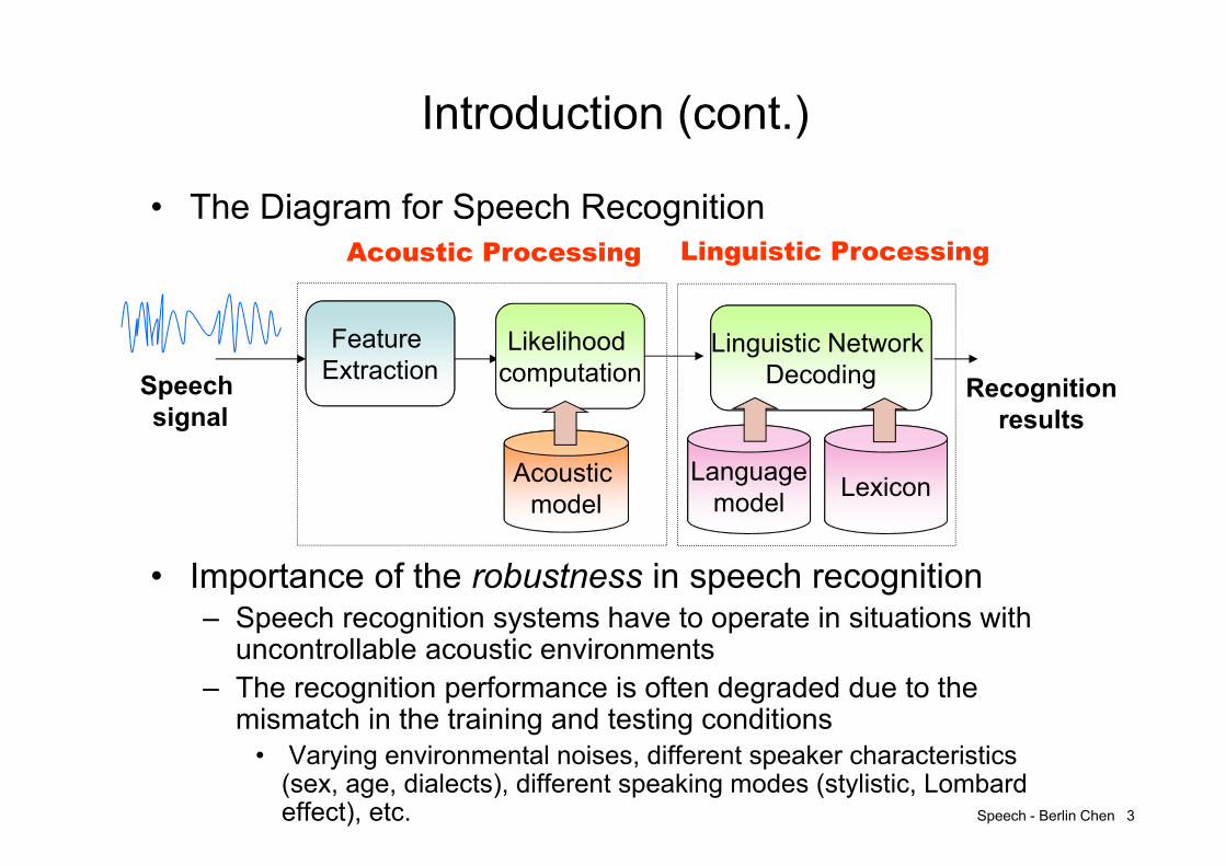
• If a speech recognition system’s accuracy does not degrade very much under mismatch conditions, the system is called robust – ASR performance is rather uniform for SNRs greater than 25dB,
but there is a very steep degradation as the noise level increases
• Signal energy measured in time domain, e.g.:
• Various noises exist in varying real-world environments– Periodic, impulsive, or wide/narrow band
1
0
*1 T
ns nsns
TE
31610log1025 5.210
N
s
N
s
EE
EEdB

Speech - Berlin Chen 5
Introduction (cont.)
• Therefore, several possible robustness approaches have been developed to enhance the speech signal, its spectrum, and the acoustic models as well
– Environmental compensation processing (feature-based)
– Acoustic model adaptation (model-based)
– Robust acoustic features (both model- and feature-based)• Or, inherently discriminative acoustic features

Speech - Berlin Chen 6
The Noise Types (1/2)
spectrum : , or
spectrumpower : , or
cos2
Re2
--
222
222
*2222
SSSSSPPPPP
NHS
NHSNHS
NHSNHSX
NHSXmnmhmsmx
nnhhssxx
NHSX
h[m]s[m]n[m]
x[m]
A model of the environment.
The Noise Types (2/2)
Speech - Berlin Chen 7
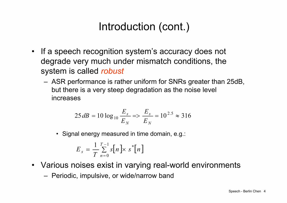
kS
kN
k
coskS
kkS sin
k
kk
kNkSkNkX
kSkNkS
kNkSkX
cos2
cossin 22
222
22
Re
Im
Speech - Berlin Chen 8
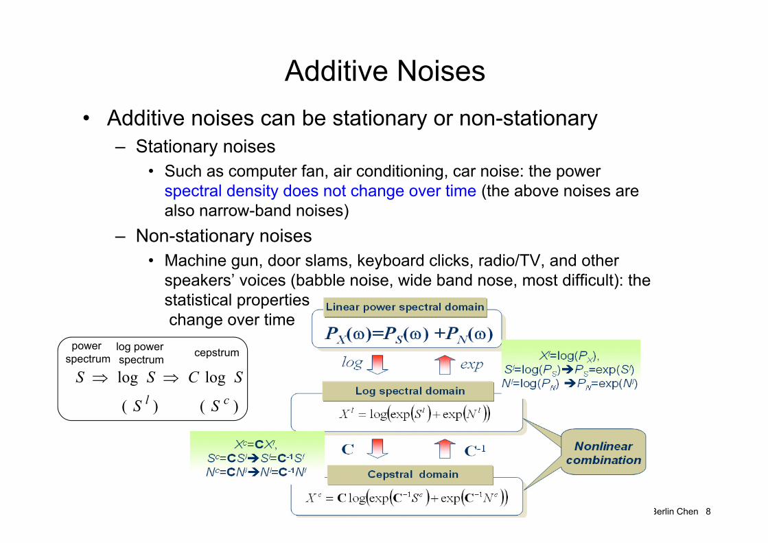
Additive Noises• Additive noises can be stationary or non-stationary
– Stationary noises• Such as computer fan, air conditioning, car noise: the power
spectral density does not change over time (the above noises are also narrow-band noises)
– Non-stationary noises• Machine gun, door slams, keyboard clicks, radio/TV, and other
speakers’ voices (babble noise, wide band nose, most difficult): the statistical propertieschange over time
) ( ) (
loglogcl SS
SCSS
powerspectrum
log powerspectrum cepstrum
Speech - Berlin Chen 9
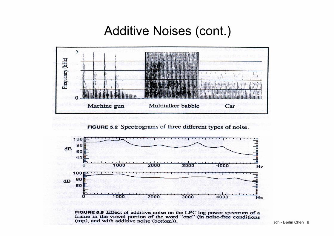
Additive Noises (cont.)

Speech - Berlin Chen 10
Convolutional Noises
• Convolutional noises are mainly resulted from channel distortion (sometimes called “channel noises”) and are stationary for most cases– Reverberation, the frequency response of microphone,
transmission lines, etc.
) ( ) (
loglogcl SS
SCSS
powerspectrum
log powerspectrum cepstrum
Speech - Berlin Chen 11
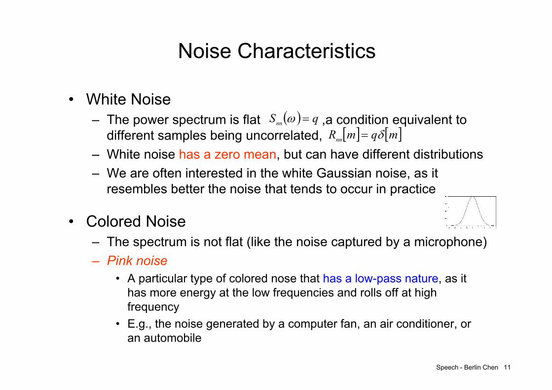
Noise Characteristics
• White Noise– The power spectrum is flat ,a condition equivalent to
different samples being uncorrelated, – White noise has a zero mean, but can have different distributions – We are often interested in the white Gaussian noise, as it
resembles better the noise that tends to occur in practice
• Colored Noise– The spectrum is not flat (like the noise captured by a microphone)– Pink noise
• A particular type of colored nose that has a low-pass nature, as it has more energy at the low frequencies and rolls off at high frequency
• E.g., the noise generated by a computer fan, an air conditioner, or an automobile
qSnn mqmRnn
Speech - Berlin Chen 12
Noise Characteristics (cont.)
• Musical Noise– Musical noise is short sinusoids (tones) randomly distributed
over time and frequency• That occur due to, e.g., the drawback of original spectral
subtraction technique and statistical inaccuracy in estimating noise magnitude spectrum
• Lombard effect– A phenomenon by which a speaker increases his vocal effect in
the presence of background noise (the additive noise)– When a large amount of noise is present, the speaker tends to
shout, which entails not only a high amplitude, but also often higher pitch, slightly different formants, and a different coloring (shape) of the spectrum
– The vowel portion of the words will be overemphasized by the speakers

A Few Robustness Approaches

Speech - Berlin Chen 14
Three Basic Categories of Approaches
• Speech Enhancement Techniques– Eliminate or reduce the noisy effect on the speech signals, thus
better accuracy with the originally trained models(Restore the clean speech signals or compensate for distortions)
– The feature part is modified while the model part remains unchanged
• Model-based Noise Compensation Techniques– Adjust (changing) the recognition model parameters (means and
variances) for better matching the noisy testing conditions– The model part is modified while the feature part remains
unchanged
• Robust Parameters for Speech– Find robust representation of speech signals less influenced by
additive or channel noise– Both of the feature and model parts are changed

Speech - Berlin Chen 15
Assumptions & Evaluations
• General Assumptions for the Noise– The noise is uncorrelated with the speech signal– The noise characteristics are fixed during the speech utterance
or vary very slowly (the noise is said to be stationary)• The estimates of the noise characteristics can be obtained during
non-speech activity – The noise is supposed to be additive or convolutional
• Performance Evaluations– Intelligibility, quality (subjective assessment)– Distortion between clean and recovered speech (objective
assessment)– Speech recognition accuracy

Speech - Berlin Chen 16
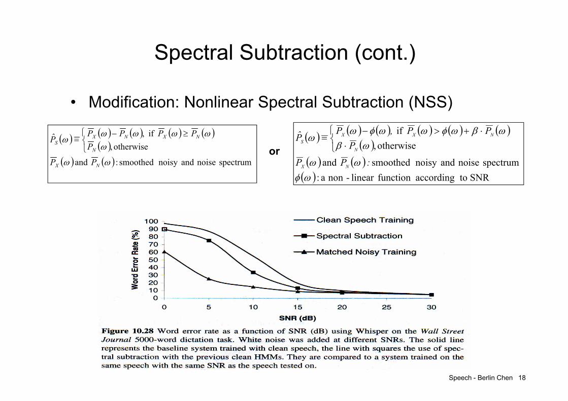
Spectral Subtraction (SS) S. F. Boll, 1979
• A Speech Enhancement Technique• Estimate the magnitude (or the power) of clean speech by
explicitly subtracting the noise magnitude (or the power) spectrum from the noisy magnitude (or power) spectrum
• Basic Assumption of Spectral Subtraction– The clean speech is corrupted by additive noise – Different frequencies are uncorrelated from each other– and are statistically independent, so that the power
spectrum of the noisy speech can be expressed as:
– To eliminate the additive noise:– We can obtain an estimate of using the average period of M
frames that are known to be just noise:
mx
ms mn
ms mn
NSX PPP
NXS PPP
NP
1M
0i i,NN PM1P
frames

Speech - Berlin Chen 17
Spectral Subtraction (cont.)
• Problems of Spectral Subtraction– and are not statistically independent such that the cross
term in power spectrum can not be eliminated– is possibly less than zero– Introduce “musical noise” when– Need a robust endpoint (speech/noise/silence) detector
ms mn
SP NX PP
Speech - Berlin Chen 18
Spectral Subtraction (cont.)
• Modification: Nonlinear Spectral Subtraction (NSS)
SNR toaccordingfunction linear -non a :
spectrum noise andnoisy smoothed and
otherwise, if
:PP
PPP,P
P
NX
N
NXXS
spectrum noise andnoisy smoothed : and
otherwise, if ,ˆ
NX
N
NXNXS
PP
PPPPP
P
or

Speech - Berlin Chen 19
Spectral Subtraction (cont.)
• Spectral Subtraction can be viewed as a filtering operation
11
:byely approximatgiven isfilter n suppressio varying timeThe
) SNR ousinstantane : ( 11
) that (supposed 1
ˆ
2/1
1
RH
PPR
RP
PPPPP
PPPPP
PPP
N
SX
NSXNS
SX
X
NX
NXS
Power Spectrum
Spectrum Domain

Speech - Berlin Chen 20
Wiener Filtering
• A Speech Enhancement Technique• From the Statistical Point of View
– The process is the sum of the random process and the additive noise process
– Find a linear estimate in terms of the process :• Or to find a linear filter such that the sequence
minimizes the expected value of
mn ms mx
ms mx
mmm nsx
llmxlh
mhmxms
][][ˆ
mh mhmxms 2msms
Noisy Speech
A linear filter h[n]
mx ms
Clean Speech

Speech - Berlin Chen 21
Wiener Filtering (cont.)
xxss
xs
lx
mm
l mm
l mm
lk
k
l
SHSkRkhkR
lkRlhkmnmskmsms
kmxlmxlhkmnkmsms
kmxlmxlhkmxms
kmxlmxlhkmxm s
khF
lmxlhms EMinimize F
0
2
• Minimize the expectation of the squared error (MMSE estimate)
t!independenlly statistica
areand m n m s
Take summation for m
Take Fourier transformm
][ and of sequences
ationautocorrel ly therespective are : and nxns
nRnR xs

Speech - Berlin Chen 22
Wiener Filtering (cont.)
• Minimize the expectation of the squared error (MMSE estimate)
) (where
filter Wiener noncausal thecalled is ,
nnssxx
nnss
ss
xx
ss
xxss
SSS
SSS
SS
H
SHS

Speech - Berlin Chen 23
Wiener Filtering (cont.)
) ousinstantane : ( 1 1
1-1-
SNRPPR,
R1
PP
PPP
SSSH
N
S
S
N
NS
S
nnss
ss
• The time varying Wiener Filter also can be expressed in a similar form as the spectral subtraction
SS vs. Wiener Filter:1. Wiener filter has stronger attenuation
at low SNR region2. Wiener filter does not invoke an
absolute thresholding
N
S
PP
log10

Speech - Berlin Chen 24
Wiener Filtering (cont.)
• Wiener Filtering can be realized only if we know the power spectra of both the noise and the signal– A chicken-and-egg problem
• Approach - I : Ephraim(1992) proposed the use of an HMM where, if we know the current frame falls under, we can use its mean spectrum as – In practice, we do not know what state each frame falls into
either• Weight the filters for each state by a posterior probability that frame
falls into each state
Sss PS or

Speech - Berlin Chen 25
Wiener Filtering (cont.)
• Approach - II :– The background/noise is stationary and its power spectrum can
be estimated by averaging spectra over a known background region
– For the non-stationary speech signal, its time-varying power spectrum can be estimated using the past Wiener filter (of previous frame)
• The initial estimate of the speech spectrum can be derived from spectral subtraction
– Sometimes introduce musical noise
,,,~
,ˆ,ˆ
,
filter) Wiener :)( index, frame :( ,,1,,ˆ
tHtPtP
PtPtPtH
HttHtPtP
XS
NS
S
XS

Speech - Berlin Chen 26
Wiener Filtering (cont.)
• Approach - III :– Slow down the rapid frame-to-frame movement of the object
speech power spectrum estimate by apply temporal smoothing
,
,, ,ˆ
,ˆ,
in ,ˆ replace to, useThen
,ˆ1,1~,
S
S
NNS
S
SS
SSS
PtPtPtH
PtPtPtH
tPtP
tPtPtP

Speech - Berlin Chen 27
Wiener Filtering (cont.)
Clean Speech
Noisy Speech
Enhanced Noise SpeechUsing Approach – III
85.0
Other more complicate Wiener filters
Speech - Berlin Chen 28
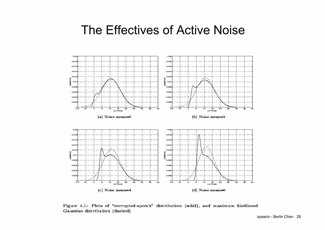
The Effectives of Active Noise

Speech - Berlin Chen 29
Cepstral Mean Normalization (CMN)
• A Speech Enhancement Technique and sometimes called Cepstral Mean Subtraction (CMS)
• CMN is a powerful and simple technique designed to handle convolutional (Time-invariant linear filtering)distortions nhnsnx
lll HSHSSHX 222 logloglog
HSX
lllll CHCSHSCCX
ll1T
0t
lt
ll1T
0tt
ll CHCSCHCST1CXCS
T1CS
and
llllllllll )2(CHCS)2(HSC2CX,)1(CHCS)1(HSC1CX :Testing :Training
channelsdifferent twofrom recored werematerialsspeech testingand training theif
llll
llll
CSCS2CX2CX
CSCS1CX1CX
The spectral characteristics of the microphone and room acoustics thus can be removed !
Time Domain
Spectral Domain
Log Power Spectral DomainCepstral Domain
Can be eliminated if the assumption of zero-mean speech contribution!

Speech - Berlin Chen 30
Cepstral Mean Normalization (cont.)
• Some Findings– Interesting, CMN has been found effective even the testing and
training utterances are within the same microphone and environment
• Variations for the distance between the mouth and the microphone for different utterances and speakers
– Be careful that the duration/period used to estimate the mean of noisy speech
• Why?– Problematic when the acoustic feature vectors are almost
identical within the selected time period

Speech - Berlin Chen 31
Cepstral Mean Normalization (cont.)
• Performance– For telephone recordings, where each call has different
frequency response, the use of CMN has been shown to provide as much as 30 % relative decrease in error rate
– When a system is trained on one microphone and tested on another, CMN can provide significant robustness

Speech - Berlin Chen 32
Cepstral Mean Normalization (cont.)
• CMN has been shown to improve the robustness not only to varying channels but also to the noise– White noise added at different SNRs– System trained with speech with the same SNR (matched
Condition)
Cepstral delta and delta-deltafeatures are computed prior to the
CMN operation so that they are unaffected.
Speech - Berlin Chen 33
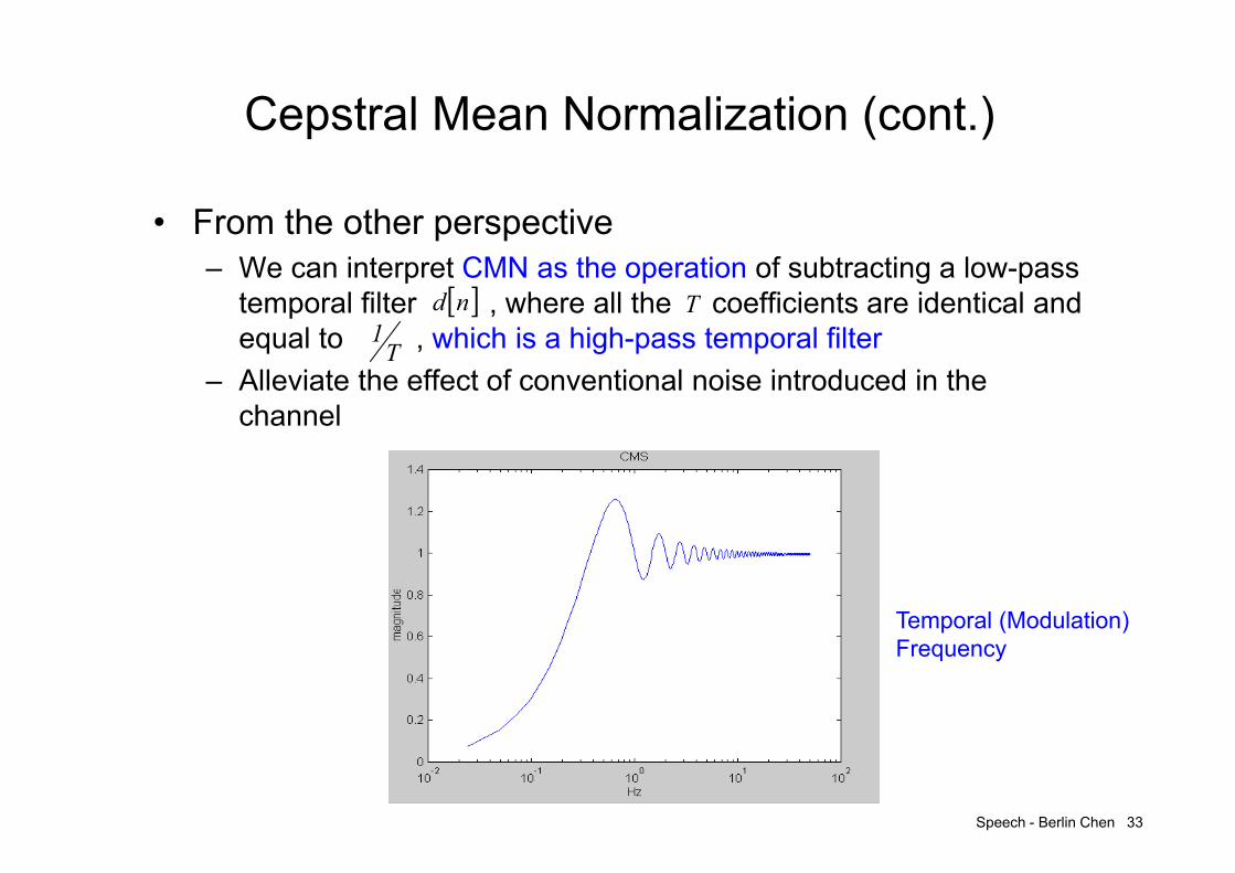
Cepstral Mean Normalization (cont.)
• From the other perspective– We can interpret CMN as the operation of subtracting a low-pass
temporal filter , where all the coefficients are identical and equal to , which is a high-pass temporal filter
– Alleviate the effect of conventional noise introduced in the channel
nd T
T1
Temporal (Modulation)Frequency

Speech - Berlin Chen 34
Cepstral Mean Normalization (cont.)
• Real-time Cepstral Normalization– CMN requires the complete utterance to compute the cepstral
mean; thus, it cannot be used in a real-time system, and an approximation needs to be used
– Based on the above perspective, we can implement other types of high-pass filters
mean) cepstral :( , tl
1tl
tl
tl CXCX1CXCX

Speech - Berlin Chen 35
Histogram EQualization (HEQ)• HEQ has its roots in the assumption that the transformed
speech feature distributions of the test (or noisy) data should be identical to that of the training (or reference) data– Find a transformation function converts to
satisfying
– Therefore, the relationship between the cumulative probability density functions (CDFs) respectively associated with the test and training speech is
dy
ydFyFpdydxxpyp TestTestTrain
)()()(1
1
xy
xF y
yFx
xFy1
)(
)(
)())((
)()(
)(1
1
yC
ydyp
ydyd
ydFyFp
xdxpxC
Train
xFyy
Train
xFTest
xTesttest
Clean Noisy0.50 0.532.10 1.951.20 1.40
-3.50 -3.204.31 4.47

Speech - Berlin Chen 36
Histogram Equalization (Cont.)
• Convert the distribution of each feature vector component of the test speech into a predefined target distribution which corresponds to that of the training speech– Attempt not only to match speech feature means/variances, but
also to completely match the feature distribution of the training and test data
1.0CDF xC Test
1.0 yC Train x
y
TestU
tterance
Reference
Distribution

Speech - Berlin Chen 37
RASTA Temporal Filter Hyneck Hermansky, 1991
• A Speech Enhancement Technique• RASTA (Relative Spectral)
Assumption– The linguistic message is coded into movements of the vocal
tract (i.e., the change of spectral characteristics)– The rate of change of non-linguistic components in speech often
lies outside the typical rate of change of the vocal tact shape• E.g. fix or slow time-varying linear communication channels
– A great sensitivity of human hearing to modulation frequencies around 4Hz than to lower or higher modulation frequencies
Effect– RASTA Suppresses the spectral components that change more
slowly or quickly than the typical rate of change of speech

Speech - Berlin Chen 38
RASTA Temporal Filter (cont.)
• The IIR transfer function
• An other version
1
4314
x
x
z98.01z2zz2z1.0
zCzC~zH
Frame index
MFCC stream H(z)H(z)
H(z)
RASTA has a peak at about 4Hz (modulation frequency)
modulation frequency 100 Hz
NewMFCC stream
tc tc~
98.01221.0 1
431
z
zzzzH
42.031.0
11.02.01~98.0~
tttttt
cccccc

Speech - Berlin Chen 39
Retraining on Corrupted Speech
• A Model-based Noise Compensation Technique• Matched-Conditions Training
– Take a noise waveform from the new environment, add it to all the utterance in the training database, and retrain the system
– If the noise characteristics are known ahead of time, this method allow as to adapt the model to the new environment with relatively small amount of data from the new environment, yet use a large amount of training data

Speech - Berlin Chen 40
Retraining on Corrupted Speech (cont.)
• Multi-style Training– Create a number of artificial acoustical environments by
corrupting the clean training database with noise samples of varying levels (30dB, 20dB, etc.) and types (white, babble, etc.), as well as varying the channels
– All those waveforms (copies of training database) from multiple acoustical environments can be used in training

Speech - Berlin Chen 41
Model Adaptation
• A Model-based Noise Compensation Technique• The standard adaptation methods for speaker adaptation
can be used for adapting speech recognizers to noisy environments– MAP (Maximum a Posteriori) can offer results similar to those of
matched conditions, but it requires a significant amount of adaptation data
– MLLR (Maximum Likelihood Regression) can achieve reasonable performance with about a minute of speech for minor mismatch. For severe mismatches, MLLR also requires a larger amount of adaptation data

Speech - Berlin Chen 42
Signal Decomposition Using HMMs
• A Model-based Noise Compensation Technique• Recognize concurrent signals (speech and noise)
simultaneously– Parallel HMMs are used to model the concurrent signals and the
composite signal is modeled as a function of their combined outputs
• Three-dimensional Viterbi Search
Clean speech HMM
Noise HMM(especially for non-stationary noise)
Computationally Expensivefor both Training and Decoding !
Speech - Berlin Chen 43
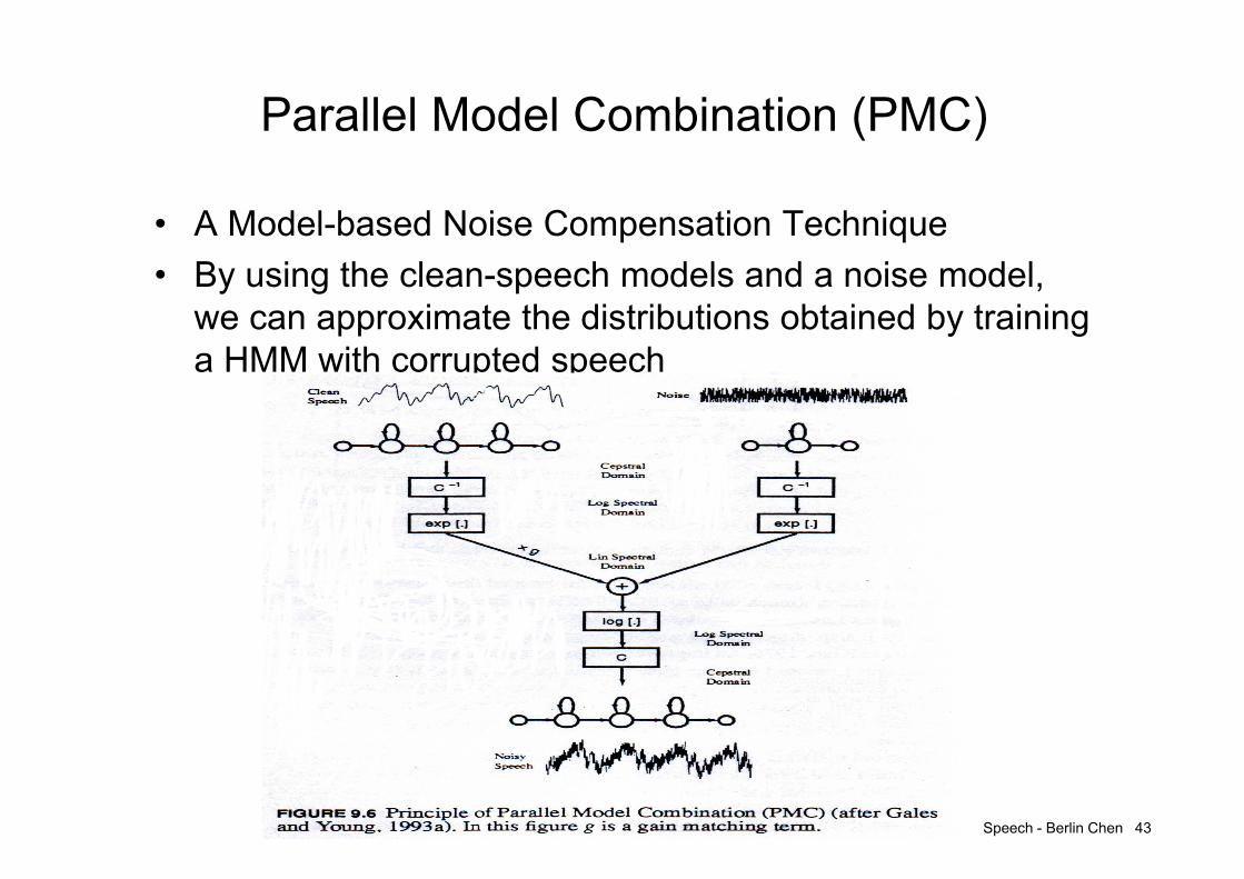
Parallel Model Combination (PMC)
• A Model-based Noise Compensation Technique• By using the clean-speech models and a noise model,
we can approximate the distributions obtained by training a HMM with corrupted speech

Speech - Berlin Chen 44
Parallel Model Combination (cont.)
• The steps of Standard Parallel Model Combination (Log-Normal Approximation)
Clean speech HMM’s
Noise HMM’s
Cepstral domainLog-spectral domain Linear spectral domain
l
l
Σμ
cl μCμ 1Tcl )( 11 CΣCΣ
2exp lii
lii
1exp lijjiij c
c
Σμ
Σμ
μμμ ~gˆ ΣΣΣ ~gˆ 2
Σ
μˆˆ
l
l
Σ
μˆˆ
c
c
Σ
μˆˆ
1log21ˆlogˆ 2ˆ
ˆ
i
iii
li
1logˆˆˆ
ˆ
ji
ijlij
lc μCμ ˆ ˆ Tlc CΣCΣ ˆ ˆ
Σμ ~ ~
Noisy speech HMM’s
In linear spectral domain, the distribution is lognormal
Because speech and noise are independent and additive in the linear spectral domain
Log-normal approximation(Assume the new distribution is lognorma
Constraint: the estimate ofvariance is positive

Speech - Berlin Chen 45
Parallel Model Combination (cont.)
• Modification-I: Perform the model combination in the Log-Spectral Domain (the simplest approximation)– Log-Add Approximation: (without compensation of variances)
• The variances are assumed to be small– A simplified version of Log-Normal approximation
• Reduction in computational load
• Modification-II: Perform the model combination in the Linear Spectral Domain (Data-Driven PMC, DPMC, or Iterative PMC)– Use the speech models to generate noisy samples (corrupted
speech observations) and then compute a maximum likelihood of these noisy samples
– This method is less computationally expensive than standard PMC with comparable performance
lll ~expexplogˆ

Speech - Berlin Chen 46
Parallel Model Combination (cont.)
• Modification-II: Perform the model combination in the Linear Spectral Domain (Data-Driven PMC, DPMC)
Noise HMM
Linear spectral domain
Clean Speech HMM
Cepstral domain
Generating samples
Domain transform
Noisy Speech HMM
Apply Monte Carlo simulation to draw random cepstral vectors(for example, at least 100 foreach distribution)

Speech - Berlin Chen 47
Parallel Model Combination (cont.)
• Data-Driven PMC

Speech - Berlin Chen 48
Vector Taylor Series (VTS) P. J. Moreno,1995
• A Model-based Noise Compensation Technique• VTS Approach
– Similar to PMC, the noisy-speech-like models is generated by combining of clean speech HMM’s and the noise HMM
– Unlike PMC, the VTS approach combines the parameters of clean speech HMM’s and the noise HMM linearly in the log-spectral domain
Power spectrum
Log Power spectrum
Non-linear function
lll
lll
HSN
HSNllllllll
HSNll
PPPHS
HS
NHS
NHSl
NHSX
eNHSfNHSfHS
eHS
ePP
PPP
PP
PPPX
PPPP
1log,, where,,,
1log
1logloglog
1log
log
logloglog
Is a vector function

Speech - Berlin Chen 49
Vector Taylor Series (cont.)
• The Taylor series provides a polynomial representation of a function in terms of the function and its derivatives at a point– Application often arises when nonlinear functions are employed
and we desire to obtain a linear approximation– The function is represented as an offset and a linear term
nnn xxoxxxfn
xxxfxxxfxfxf
RRf
000
200000
!1....
21
:

Speech - Berlin Chen 50
Vector Taylor Series (cont.)
• Apply Taylor Series Approximation
– VTS-0: use only the 0th-order terms of Taylor Series– VTS-1: use only the 0th- and 1th-order terms of Taylor Series– is the vector function evaluated at a particular
vector point
• If VTS-0 is used
.....
,,,,
,,,,,,
0000
0000
0000
000
lll
lllll
l
lll
lll
lllllllll
NNdN
NHSdfHH
dHNHSdf
SSdS
NHSdfNHSfHSNf
t)independen are and (if
Gaussian) also is (
lllll
llllll
lllll
llllll
llllll
HSXu,u,ufuu
u,u,ufEuuN,H,SfEuuu
N,H,SfHSEXE
hsx
nhshs
nhshs
hsx
Gaussian) also is ( domain spectrumpower log in the
, ,(constant) bias a asit regardcan weinvariant, time-linear isfilter channel theIf
ll
lllll Xu,g,ufguu
g
sx
nssx
0-th order VTS
lll NHSf 000 ,,
To get the clean speech statistics
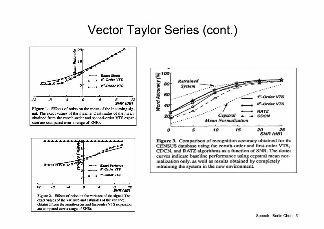
Speech - Berlin Chen 51
Vector Taylor Series (cont.)

Speech - Berlin Chen 52
Retraining on Compensated Features
• A Model-based Noise Compensation Technique that also Uses enhanced Features (processed by SS, CMN, etc.)– Combine speech enhancement and model compensation
SPLICE: Stereo-based Piecewise Linear Compensation

More on SPLICE
Speech - Berlin Chen 53Note that this slide was adapted from Dr. Droppo’s presentation slides

Speech - Berlin Chen 54
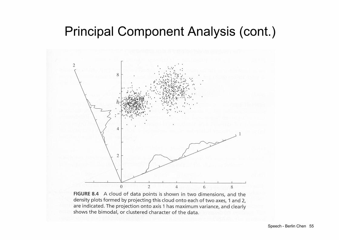
Principal Component Analysis
• Principal Component Analysis (PCA) :– Widely applied for the data analysis and dimensionality reduction
in order to derive the most “expressive” feature– Criterion:
for a zero mean r.v. xRN, find k (kN) orthonormal vectors{e1, e2,…, ek} so that
– (1) var(e1T x)=max 1
(2) var(eiT x)=max i
subject to ei ei-1 …… e1 1 i k
– {e1, e2,…, ek} are in fact the eigenvectors of the covariance matrix (x) for xcorresponding to the largest k eigenvalues
– Final r.v y R k : the linear transform (projection) of the original r.v., y=ATxA=[e1 e2 …… ek]
Principal axis
Speech - Berlin Chen 55
Principal Component Analysis (cont.)
Speech - Berlin Chen 56
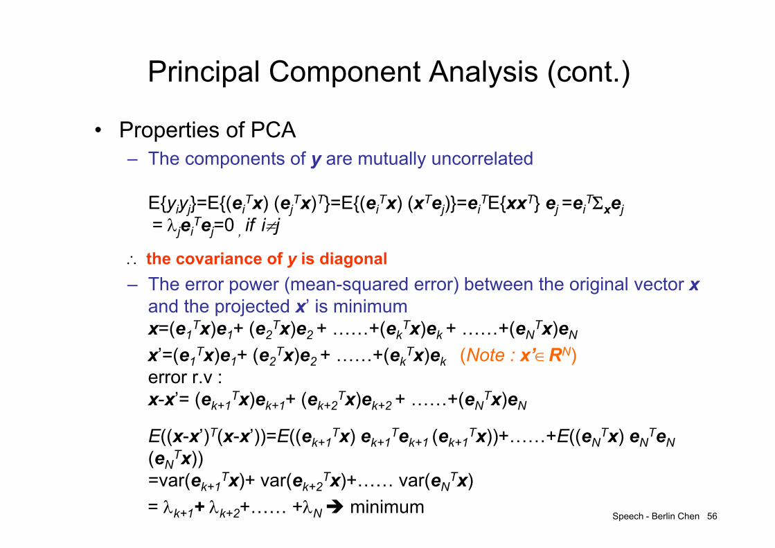
Principal Component Analysis (cont.)
• Properties of PCA– The components of y are mutually uncorrelated
E{yiyj}=E{(eiTx) (ej
Tx)T}=E{(eiTx) (xTej)}=ei
TE{xxT} ej =eiTxej
= jeiTej=0 , if ij
the covariance of y is diagonal– The error power (mean-squared error) between the original vector x
and the projected x’ is minimum x=(e1
Tx)e1+ (e2Tx)e2 + ……+(ek
Tx)ek + ……+(eNTx)eN
x’=(e1Tx)e1+ (e2
Tx)e2 + ……+(ekTx)ek (Note : x’RN)
error r.v : x-x’= (ek+1
Tx)ek+1+ (ek+2Tx)ek+2 + ……+(eN
Tx)eN
E((x-x’)T(x-x’))=E((ek+1Tx) ek+1
Tek+1 (ek+1Tx))+……+E((eN
Tx) eNTeN
(eNTx))
=var(ek+1Tx)+ var(ek+2
Tx)+…… var(eNTx)
= k+1+ k+2+…… +N minimum

Speech - Berlin Chen 57
PCA Applied in Inherently Robust Features
• Application 1 : the linear transform of the originalfeatures (in the spatial domain)
Original feature stream xt
Frame index
AT AT AT AT
transformed feature stream zt
Frame index
zt= ATxt
The columns of A are the “first k” eigenvectors of x
Speech - Berlin Chen 58
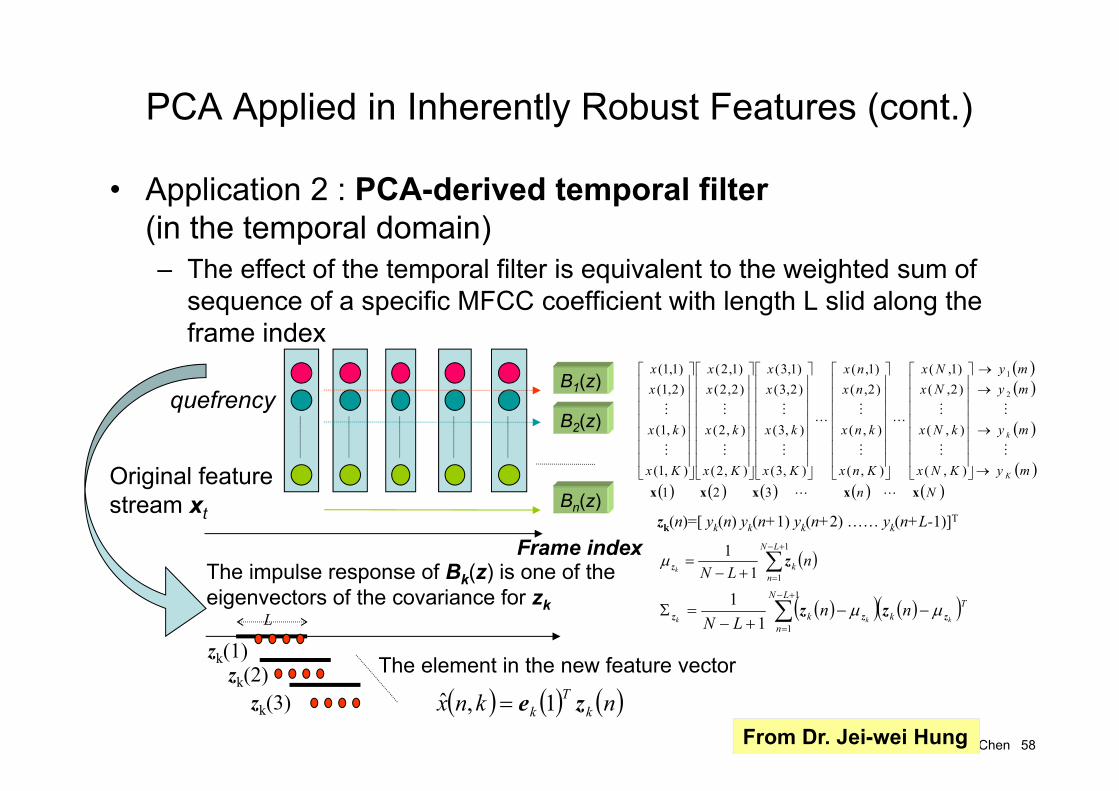
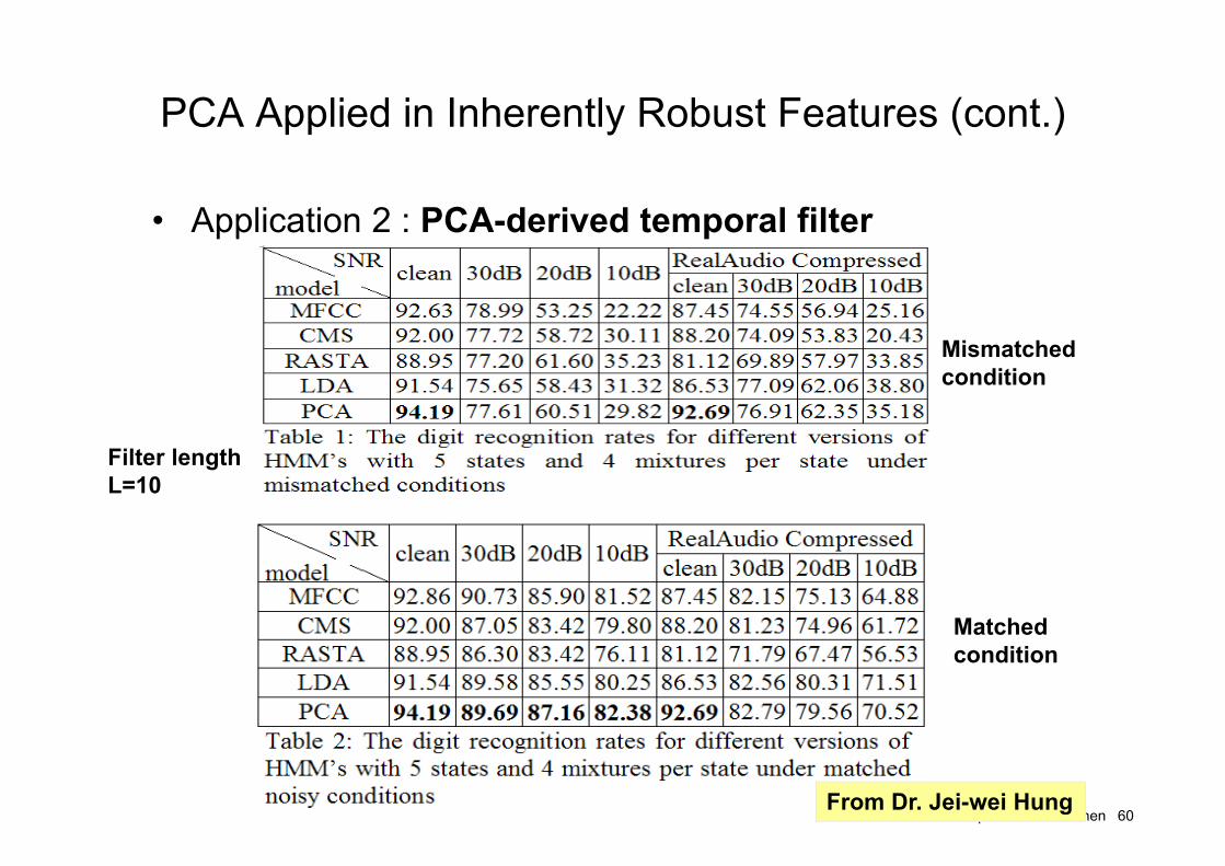
PCA Applied in Inherently Robust Features (cont.)
• Application 2 : PCA-derived temporal filter(in the temporal domain)– The effect of the temporal filter is equivalent to the weighted sum of
sequence of a specific MFCC coefficient with length L slid along the frame index
quefrency
Frame index
B1(z)
B2(z)
Bn(z)
L
zk(1)zk(2)
zk(3)
Original feature stream xt
The impulse response of Bk(z) is one of the eigenvectors of the covariance for zk
Nn
my
my
mymy
KNx
kNx
NxNx
Knx
knx
nxnx
Kx
kx
xx
Kx
kx
xx
Kx
kx
xx
K
k
xxxxx 3 2 1 ),(
),(
)2,()1,(
),(
),(
)2,()1,(
),3(
),3(
)2,3()1,3(
),2(
),2(
)2,2()1,2(
),1(
),1(
)2,1()1,1(
2
1
zk(n)=[ yk(n) yk(n+1) yk(n+2) …… yk(n+L-1)]T
1
111 LN
nk n
LNkzz
1
111 LN
n
Tkk kkk
nnLN zzz zz
nknx kT
k ze 1,ˆ
The element in the new feature vector
From Dr. Jei-wei Hung

Speech - Berlin Chen 59
PCA Applied in Inherently Robust Features (cont.)
The frequency responses of the 15 PCA-derived temporal filters
From Dr. Jei-wei Hung
Speech - Berlin Chen 60
PCA Applied in Inherently Robust Features (cont.)
• Application 2 : PCA-derived temporal filter
From Dr. Jei-wei Hung
Mismatched condition
Matched condition
Filter lengthL=10

Speech - Berlin Chen 61
PCA Applied in Inherently Robust Features (cont.)
• Application 3 : PCA-derived filter bankPower spectrumobtained by DFT
x1 x2 x3
h1
h3
h2 hk is one of the eigenvectors of the covariancefor xk
From Dr. Jei-wei Hung

Speech - Berlin Chen 62
PCA Applied in Inherently Robust Features (cont.)
• Application 3 : PCA-derived filter bank
From Dr. Jei-wei Hung

Speech - Berlin Chen 63
Linear Discriminative Analysis
• Linear Discriminative Analysis (LDA)– Widely applied for the pattern classification – In order to derive the most “discriminative” feature– Criterion : assume wj, j and j are the weight, mean and
covariance of class j, j=1……N. Two matrices are defined as:
Find W=[w1 w2 ……wk]such that
– The columns wj of W are the eigenvectors of Sw
-1SBhaving the largest eigenvalues
Nj jjw
Nj
Tjjjb
w
w
1
1
: covariance class-Within
: covariance class-Between
ΣS
μμμμS
WSW
WSWW
Ww
T
bT
maxargˆ
Speech - Berlin Chen 64
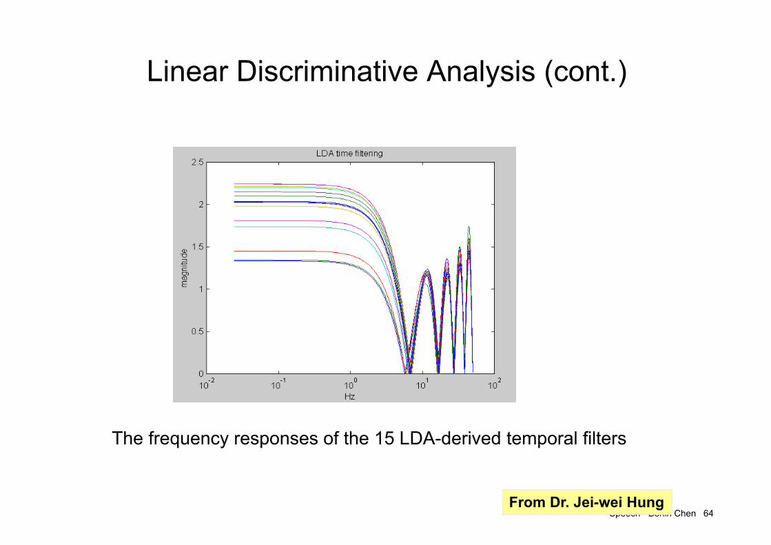
Linear Discriminative Analysis (cont.)
The frequency responses of the 15 LDA-derived temporal filters
From Dr. Jei-wei Hung

Speech - Berlin Chen 65
Minimum Classification Error
• Minimum Classification Error (MCE):– General Objective : find an optimal feature presentation or an
optimal recognition model to minimize the expected error of classification
– The recognizer is often operated under the following decision rule :C(X)=Ci if gi(X,)=maxj gj(X,)={(i)}i=1……M (M models, classes), X : observations,gi(X,): class conditioned likelihood function, for example,
gi(X,)=P(X|(i))– Traditional Training Criterion :
find (i) such that P(X|(i)) is maximum (Maximum Likelihood) if X Ci
• This criterion does not always lead to minimum classification error, since it doesn't consider the mutual relationship between different classes
• For example, it’s possible that P(X|(i)) is maximum but X Ci

kCXXLRP kCXXLRP
kLR
k
kCX kCX XLR
Speech - Berlin Chen 66
Minimum Classification Error (cont.)
Type I error
Type II error
Threshold
Example showing histograms of the likelihood ratio when the observation and
Type I error: False RejectionType II error: False Alarm/False Acceptance

Speech - Berlin Chen 67
Minimum Classification Error (cont.)
• Minimum Classification Error (MCE) (Cont.):– One form of the class misclassification measure :
– A continuous loss function is defined as follows :
– Classifier performance measure :
0)(error tion classificacorrect a implies 0
1)(errorication misclassif a implies 0
,exp1
1log,1
XdXd
CXXgM
XgXd
i
i
iij
iii
ddlfunctionsigmoidthewhere
CXXdlXl iii
exp11
,
X
M
iiiX CXXlXLEL
1
,,

Speech - Berlin Chen 68
Minimum Classification Error (cont.)
• Using MCE in model training : – Find such that
the above objective function in general cannot be minimized directly but the local minimum can be achieved using gradient decent algorithm
• Using MCE in robust feature representation
,minargminargˆ XLEL X
: ,1
ofparameterarbitraryanww
Lww tt
yaccordingl changed also is model thechanged, is onpresentati feature while: feature original theof ma transfor :
,minargˆ
NoteXf
XfLEf fXf