Robustfaultestimationofuncertainsystemsusing anLMI ...mece2hv/Papers/t_pdf5.pdf · DOI:...

INTERNATIONAL JOURNAL OF ROBUST AND NONLINEAR CONTROLInt. J. Robust Nonlinear Control 2008; 18:1657–1680Published online 27 March 2008 in Wiley InterScience (www.interscience.wiley.com). DOI: 10.1002/rnc.1313

Robust fault estimation of uncertain systems usingan LMI-based approach

Euripedes G. Nobrega1, Musa O. Abdalla2,∗,† and Karolos M. Grigoriadis3

1Departamento de Mecanica Computacional, Universidade Estadual de Campinas, Campinas, SP, Brazil2Mechanical Engineering Department, University of Jordan, Amman, Jordan3Mechanical Engineering Department, University of Houston, Houston, U.S.A.

SUMMARY

General recent techniques in fault detection and isolation (FDI) are based on H∞ optimization methodsto address the issue of robustness in the presence of disturbances, uncertainties and modeling errors.Recently developed linear matrix inequality (LMI) optimization methods are currently used to designcontrollers and filters, which present several advantages over the Riccati equation-based design methods.This article presents an LMI formulation to design full-order and reduced-order robust H∞ FDI filtersto estimate the faulty input signals in the presence of uncertainty and model errors. Several cases areexamined for nominal and uncertain plants, which consider a weight function for the disturbance and areference model for the faults. The FDI LMI synthesis conditions are obtained based on the boundedreal lemma for the nominal case and on a sufficient extension for the uncertain case. The conditions forthe existence of a feasible solution form a convex problem for the full-order filter, which may be solvedvia recently developed LMI optimization techniques. For the reduced-order FDI filter, the inequalitiesinclude a non-convex constraint, and an alternating projections method is presented to address this case.The examples presented in this paper compare the simulated results of a structural model for the nominaland uncertain cases and show that a degree of conservatism exists in the robust fault estimation; however,more reliable solutions are achieved than the nominal design. Copyright q 2008 John Wiley & Sons, Ltd.

Received 30 March 2006; Revised 18 January 2008; Accepted 21 January 2008

KEY WORDS: fault detection and isolation; linear matrix inequalities; robust H∞ filtering; linear systems

1. INTRODUCTION

The increasing complexity of engineering systems demands higher safety and reliability, leadingto the need for fault detection (FD) and fault tolerant control (FTC) methods. Monitoring and

∗Correspondence to: Musa O. Abdalla, Mechanical Engineering Department, University of Jordan, Amman, Jordan.†E-mail: [email protected]

Contract/grant sponsor: FAPESP

Copyright q 2008 John Wiley & Sons, Ltd.

1658 E. G. NOBREGA, M. O. ABDALLA AND K. M. GRIGORIADIS

diagnosing faults in a system is an important objective in itself, but in an FTC system, the outputsignals from fault detection and isolation (FDI) modules may also be used to reconfigure thecontroller module in order to accommodate the fault. To develop FD methods, much effort hasbeen dedicated since the pioneer works of Beard [1] and Jones [2], but the number of real FTC orFDI applications is very low till today. The functions of monitoring and diagnosing systems arenecessary to provide early warning of faulty sensors, actuators or system components, avoidingeconomical loss or dangerous situations for operators or users. Some surveys of the FDI methods[3–6] and books present the basics of the many different methods developed to detect faults [7, 8].

Early FDI methods were based on hardware redundancy to reveal malfunctions in sensors oractuators. However, these methods are expensive and their use will be gradually reduced as theanalytical methods are becoming more reliable. For critical systems, e.g. aircrafts, satellites, deep-space probes, etc., combinations of both approaches shall reduce the number of redundant hardwarecomponents. Analytical redundancy methods for FDI are based on the comparison of the actualmeasured and expected signals, the so-called residuals, generated through established relationsbetween input and output signals. These methods may be classified into two broad categories,model-based or knowledge-based, which use, respectively, mathematical modeling of the monitoredsystem or some logical description of the measured signals and its components [4].

In general, two separate processes are necessary: residual generation and residual evaluation.The residual signals must be small if no fault is present and must become significant if there isa fault. The first process compares the redundant signals to generate the residuals. The secondprocess aims at evaluating the residual signals in order to achieve three different tasks: detection,isolation and identification of possible faults [3], or, in other words, trigger an alarm when a faultis present, localize it and determine its severity. During the first two decades, some aspects ofmodel-based methods have been the main research themes, such as unknown inputs estimation,how to reduce the influence of disturbances on the residuals and how to maximize its sensitivity tofaults. The work turned during the 1990s to adapting control methods such as H2 and H∞ [9–14],trying to make the residuals sensitive to faults but insensitive to disturbances and solving theproblem through Riccati equations. However, only a mathematical nominal model of the systemis usually available, not necessarily considering the presence of exogenous disturbance inputs andnoise, and also time-varying parameters and non-modeled plant dynamics. The focus has so beenaddressed to the search of FDI methods applied to dynamic uncertain systems with modelingerrors and unknown inputs. The goals of a current FDI method are to make the residuals notonly sensitive to faults and insensitive to disturbances but also robust to dynamical uncertaintiesand uncertain or time-varying parameters. It is obvious, though, that some frequency distributiondifferences between the exogenous inputs and faults are necessary, in order to be possible todiscriminate the unknown input signals from the faults, through processing of the measured outputsand the generated residuals. The present work intends to contribute to the robust design of model-based FDI filters for systems presenting parameter and dynamic uncertainties, adopting a linearmatrix inequality (LMI)-based approach to solve the problem. Some commentaries about recentdevelopments are presented next.

Among the significant new topics that arose in the last years, the H−-index is concernedwith the performance ratio between unknown disturbance and residual sensitivity. The initialapproach [15] considered the relationship between the H− index (regarding that it is not a norm)of the transfer function of the fault vector to the residual and the H∞-norm of the transferfunction of the disturbance vector to the residual, leading to a mixed index problem. Extendingthis formulation, including the uncertain external loop, the work of Chen and Patton [13] presents

Copyright q 2008 John Wiley & Sons, Ltd. Int. J. Robust Nonlinear Control 2008; 18:1657–1680DOI: 10.1002/rnc

ROBUST FAULT ESTIMATION OF UNCERTAIN SYSTEMS 1659

a more complete development, with the solution for the observer based on the �-analysis method.Adopting the same mixed index formulation, using an LMI approach, but not including the uncertainloop, the configuration presented in Rambeaux et al. [16] makes use of extra dynamics throughfiltering the output of the observer, leading to better sensitivity of the detector.

Some authors adopted parametric uncertain systems using a polytopic representation for theuncertainties. Hamelin and Sauter [17] presented a frequency domain procedure based on interval-type parameter uncertainties, leading to a polytopic unstructured uncertain model of the system.Also using the frequency domain, Casavola et al. [18] formulated the FDI filter design problemwith two objectives for polytopic uncertain LTI systems, not needing to know a nominal plantmodel. The objectives are to minimize the H∞-norm of the disturbance to residual map and themaximization of the lowest singular value of the residual to faults map over a prescribed frequencyrange. This renders a non-convex constraint, which may be recast into a convex one, throughthe linearization of the corresponding feasibility region, resulting in a quasi-LMI problem. Theprojection lemma and congruence transformations are used to solve the problem. Frisk and Nielsen[19] address the problem of robust residual generation in the presence of parametric uncertaintiesand deterministic disturbances that influence the process, focusing on the designing dealing withparametric uncertainty in a structured residual framework.

Separating the formulation as different objectives has been another common approach. A mixedH2 and H∞ residual generator is proposed by Khosrowjerdi et al. [20], assuming fixed spectraldensities for the unknown disturbances treated as an H2 objective and bounded energy for theuncertain input formulated as an H∞ filtering problem. The authors justify their options consideringthat the H2-norm cannot guarantee robustness, whereas the H∞-norm can reduce sensitivity tofaults but provides robustness to the uncertainties. The main advantage is the possibility of adjustingthe trade-off between detection performance and noise sensitivity through a single parameter. AnFDI filter for uncertain systems with modeling errors and disturbance inputs, using a two observersapproach, is presented by Zhong et al. [21], for a sub-divided state space. The first part of thestate variable is only affected by plant input and unknown disturbances, and the second part isonly affected by faults. A two-objective H∞ respective problem is formulated and solved usingan LMI technique.

Recently, presenting a more complete treatment of uncertain systems and also a multi-objectivedesign method, the approach of Henry and Zolghadri [22] imposes sensitivity to faults through anH−-index over specified frequency ranges and H∞ performance to enforce robustness to modeluncertainty. It also included additional requirements of regional poles assignment for the FD filter,searching to tune the transient response and a decay rate of the residual.

To enforce the frequency behavior of the FDI filter, Frisk and Nielsen [23] introduced the ideaof using a reference model in an FDI framework. Considering that the performance of the FDIfilter should be devised as a trade-off between robustness to modeling errors and insensitivityto unknown inputs, Zhong et al. [24] reduced the design problem to a standard model-matchingone, through a reference system obtained from nominal design and the synthesis of the filterminimizing the H∞-norm of the difference between the reference model and the residual generatoroutput. The unknown input vector includes disturbances, uninterested fault and some norm-boundedunstructured model uncertainties. The authors consider the major difficulty to be the selection ofa reference model with physical meaning from the FDI viewpoint.

Another recent approach is to impose directly as the residuals, the estimation of the fault signalsthemselves, instead of the differences produced in the output signals [25]. This has the advantage ofeasily isolating the fault and can be accomplished through a slight change in the index, permitting



the adoption of H∞ methods to design the filters. The problem easily fits in a standard H∞optimization control setup, and the observer and the output filter are computed in a single step.

Robust estimation of the faulty input signals is the method adopted in the present work.A thorough treatment of robustness involving parametric and dynamic uncertainties through input–output signals representation is adopted, in the sense usually found in the robust controller designarea. The proposed method may also be used to design an output observer and achieve FD in amore common type of residual. But considering that FD signals may be part of an FTC system,it is reasonable to expect a better performance from the controller if the fault signals are esti-mated, instead of a combination of signals without specific significance. An LMI solution ofthe H∞ filter has been published [26, 27], and the general robust treatment for H∞ filter design[28], and they were adapted to robust FDI filter design and formulated as a new set of LMIs.A complete LMI-based approach to estimate the input fault vector using H∞ filtering is presentedfor the continuous-time FDI nominal and robust problems. The proposed formulation allows thedevelopment of necessary and sufficient solvability conditions for the fixed-order FDI filter design.The full-order H∞ FDI filter design is characterized in terms of convex LMIs whose solution isparameterized for all admissible filters, for nominal and uncertain plants. The reduced-order H∞filter design is characterized by LMIs with additional coupling non-convex matrix rank constraints,and for this case, an alternating projections method is presented that may be applied for both thenominal and uncertain cases. Some simulation examples for a structural system are presented todemonstrate the proposed methods.

The notation used in this work is standard. The transpose of a real matrix A is denoted by AT, andthe symbols >,� (<,�) are used to denote positive (negative) definite and semidefinite matrices.The H∞ norm of a rational transfer function F(s) is defined as ‖F(s)‖∞ =max� �(F( j�)), where�(·) denotes the maximum singular value of a matrix. The L2 norm of a vector-valued functionf (t), is defined as ‖ f (t)‖L2 ={∫∞

0 f T(t) f (t)dt}1/2. The induced matrix norm is given as ‖A‖=�(A)={�max(AAT)}1/2. Given a real n×m matrix A with rank r , an orthogonal complement A⊥is defined as the possibly non-unique matrix that satisfies A⊥A=0 and A⊥A⊥T>0. Hence, theorthogonal complement may be computed from the singular-value decomposition of a matrix

A=[U1 U2][

�1 0

0 0

][V T1

V T2

]

as A⊥ =TUT2 where T is an arbitrary non-singular matrix. Linear fraction transformations (LFT)

are used to represent the plants to be monitored. Considering the matrices F and S=[S11S21

S12S22

],

the lower LFT is defined as Fl(S,F)= S11+S12F(I −S22F)−1S21, for appropriately dimensionedmatrices and admitting that the inverse exists.

2. NOMINAL PROBLEM FORMULATION

In this section, the nominal H∞ FDI filtering problem is formulated based on the LFT form.The corresponding LMIs and their solutions for the full-order problem are presented. Also, analgorithm is proposed to solve the reduced-order problem.



2.1. LFT modeling

Consider a system plant P of order np with its state-space representation

xp = Apxp+Bpu+Epd+Fp f

yp = Cpxp+Dpu+Gpd+Hp f(1)

where xp is the state vector, u is the control input, d is the disturbance vector, f is the fault vectorand Ap, Bp,Cp,Dp,Ep, Fp,Gp and Hp are real matrices of appropriate dimensions. Fp and Hp aredistribution matrices that model actuator, component and sensor additive faults. The block diagramdepicted in Figure 1 represents the proposed configuration.

In Figure 1, P represents the plant to be monitored and F is the unknown filter that is to bedetermined. The estimation error is defined as e=r− f , where r is the residual-generated vectorof the FDI filter F . Our objective is to design a filter F such that r provides an estimate of the faultvector f . By examining the patterns and properties of vector r , FTC or detection and isolation offaults for monitoring purposes can be accomplished.

Based on the above formulation, the proposed H∞ optimal filtering problem is to find an FDIdynamic filter F to minimize the worst-case estimation error energy ‖e‖L2 over all bounded energygeneralized disturbance wT=[uT dT f T], that is

minF

supw∈L2−{0}

‖e‖L2

‖w‖L2

(2)

Adopting the index in (2) is equivalent to minimizing the H∞ norm of the transfer function Twebetween the generalized disturbance input and the error of the fault estimation. The �-suboptimalH∞ FDI filtering problem is to find (if exists) a filter such that ‖Twe‖∞<�, where � is a givenpositive scalar.

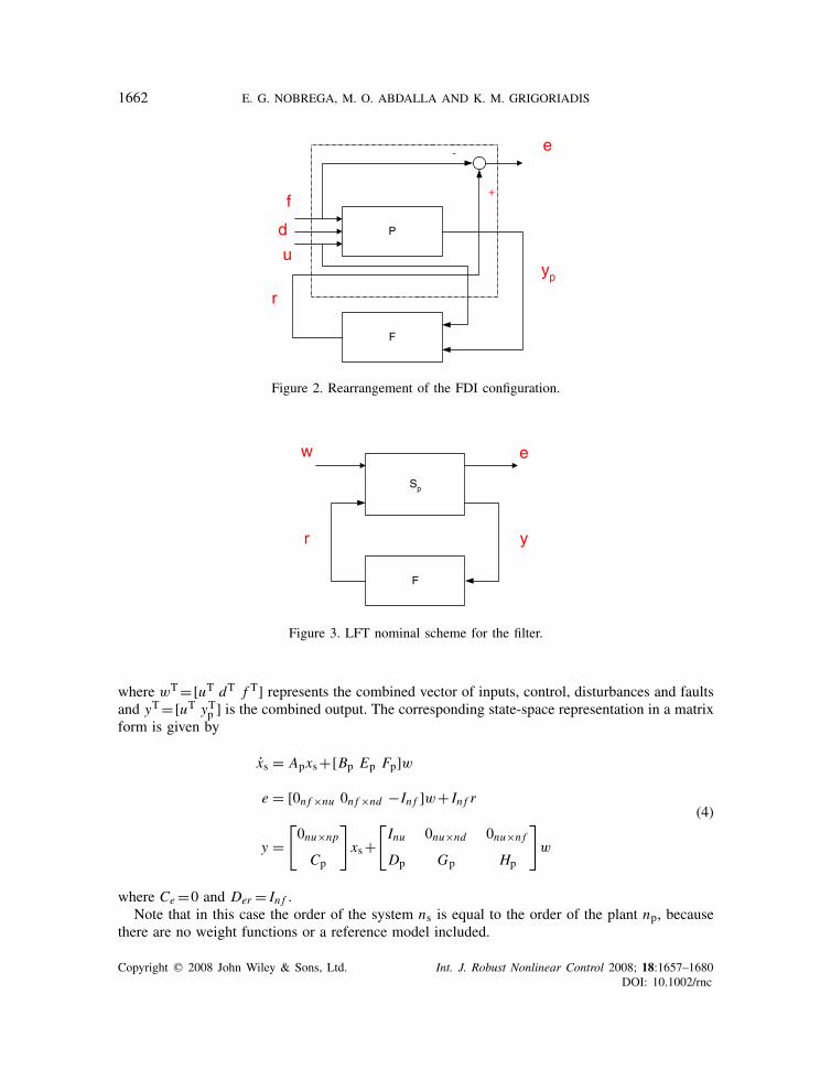
The block diagram in Figure 1 can be rearranged as presented in Figure 2. Weighting functionscan be used to shape appropriately the frequency content of the input signals for better FD anddisturbance rejection and can be easily taken into account in the formulation.

In Figure 3, the resultant LFT representation for the nominal plant is presented. Using thesefigures and considering the state-space formulation as

xs = Asxs+Bww

e = Cexs+Deww+Derr

y = Cyxs+Dyww

(3)

PF

f

d

ey

+-

u r

Figure 1. Proposed FDI filter scheme.



f

d P

F

e

yp

+

-

r

u

Figure 2. Rearrangement of the FDI configuration.

w

Sp

F

e

yr

Figure 3. LFT nominal scheme for the filter.

where wT=[uT dT f T] represents the combined vector of inputs, control, disturbances and faultsand yT=[uT yTp ] is the combined output. The corresponding state-space representation in a matrixform is given by

xs = Apxs+[Bp Ep Fp]w

e = [0n f ×nu 0n f ×nd −In f ]w+ In f r

y =[0nu×np

Cp

]xs+

[Inu 0nu×nd 0nu×n f

Dp Gp Hp

]w

(4)

where Ce=0 and Der = In f .Note that in this case the order of the system ns is equal to the order of the plant np, because

there are no weight functions or a reference model included.



2.2. Continuous-time FDI filter design

To solve the nominal filter design problem using an LMI-based approach in the continuous-timedomain, some algebraic results are presented. Consider a stable nsth-order linear time-invariantsystem with the following state-space representation:

xs = Asxs+Bww

e = Deww+r

y = Cyxs+Dyww

(5)

where xs is the state vector, y is the output vector, w is the generalized disturbance vector andAs, Bw, Dew,Cy and Dyw are real matrices of appropriate dimensions. It is our objective to designa stable linear dynamic filter with the following state-space representation:

xf = Afxf+Bfy

r = Cfxf+Dfy(6)

where the output r is the estimated fault vector. The vector xf is the filter state vector, and Af, Bf,Cf,and Df are real matrices of appropriate dimensions to be computed. The order of the filter nf isrestricted to be less than or equal to the order of the system ns.

An LMI-based H∞ approach will be used to find filter F . The filter design is based on thebounded real lemma [29], which is presented next.

Lemma 1Consider a stable linear time-invariant system with state-space model

x = Acx+Bcw

y = Ccx+Dcw(7)

with transfer function Tc(s)=Cc(s I −Ac)−1Bc+Dc and let � be a given positive scalar. Then

‖Tc‖∞<� if and only if there exists a matrix P>0 that satisfies

⎡⎢⎢⎣PAc+AT

c P PBc CTc

BTc P −�2 I DT

c

Cc DTc −I

⎤⎥⎥⎦<0 (8)

To find the solvability conditions of the LMI problem in inequality (8), the following lemmamay be applied [29].Lemma 2Let �, � and �=�T be given matrices. There exists a matrix F to solve the matrix inequality

�F�+�TFT�T+�<0 (9)



if and only if the following conditions are satisfied:

�⊥��⊥T < 0 (10)

�T⊥��T⊥T < 0 (11)

These two lemmas may be applied for the case of nominal H∞ FDI filtering to provide thenecessary and sufficient conditions for the existence of such filters and the parameterization of allsolutions. The following theorem gives the solution to the �-suboptimal H∞ FDI filtering problem.

Theorem 1There exists an nfth-order filter F to solve the �-suboptimal H∞ FDI filtering problem if and onlyif there exist matrices X and Y with Y�X>0 such that the following conditions are satisfied:

[X As+AT

s X XBw

BTwX −�2 I

]< 0 (12)

[CTy

DTyw

]⊥[Y As+AT

s Y Y Bw

BTwY DT

ewDew −�2 I

][CTy

DTyw

]⊥T

< 0 (13)

rank(X−Y ) � nf (14)

The proof of this theorem is presented in Appendix A.

For the full-order FDI filter design (nf=ns), the rank constraint represented by inequality (14)is automatically satisfied and it is not necessary to be included in the formulation. However, theplant order increases when a weighting function or a reference model is included, demanding areduced-order FDI filter design (nf<ns). This is also a common requirement for complex high-order plants. In this case, the rank constraint renders a non-convex problem, demanding alternatemethods to solve the system.

To provide a parameterization of all feasible filters, consider the error system Fl(Sp,F) fromthe LFT scheme of Figure 3. Defining the state-space vector as xT=[xTs xTf ], this error system isdescribed by the following state-space equations:

x =[

As 0

BfCy Af

]x+

[Bw

BfDyw

]w

e = [DfCy Cf]x+[Dew +DfDyw]w

This system can be rewritten as

x = (A0+BFM)x+(B0+BFE)w

e = (C0+HFM)x+(D0+HFE)w



for the respective matrices

A0 =[As 0

0 0

], B0=

[Bw

0

], C0=0, D0=Dew

B =[0 0

0 I

], M=

[Cy 0

0 I

], E=

[Dyw

0

], H =[I 0]

(15)

where the unknown filter matrix is defined as

F=[Df Cf

Bf Af

]

Applying Lemma 1, the inequality in (8) becomes⎡⎢⎢⎣P(A0+BFM)+(A0+BFM)TP P(B0+BFE) (HFM)T

(B0+BFE)TP −�2 I (D0+HFE)T

HFM D0+HFE −I

⎤⎥⎥⎦<0

Using Lemma 2, it can be easily devised from (9) that

�=⎡⎢⎣PB

0

H

⎤⎥⎦ , �T=

⎡⎢⎢⎣MT

ET

0

⎤⎥⎥⎦ and �=

⎡⎢⎢⎣PA0+AT

0 P PB0 0

BT0 P −�2 I DT

0

0 D0 −I

⎤⎥⎥⎦ (16)

Considering the definitions in (16), the following result provides a parameterization of all feasiblefilters based on the solution (X,Y ) of the FDI solvability conditions (12)–(14).

Theorem 2All the �-suboptimal H∞ FDI nth-order filters F that correspond to a feasible matrix pair (X,Y )

are given by

F=[Df Cf

Bf Af

]=−R−1�T��T�+�1/2 J�1/2

where �, R and J are free matrix parameters subject to

�=(�R−1�T−�)−1>0, R>0, ‖J‖<1

� and � defined by

� = R−1−R−1�T(�−��T��)�R−1

� = (��)−1

The proof is not presented here but follows the same approach as in Grigoriadis and Watson[26]. Theorem 2 provides a set of solutions that guarantees the H∞ norm bound for the system.The free parameters may be used then to optimize other system properties.



2.3. Reduced-order filter design via alternating projections

In the previous section, the continuous-time full-order FDI filter design has produced convex LMIconstraints, represented by inequalities (12) and (13). On the other hand, the reduced-order FDIfilter design requires the inclusion of the rank constraint, inequality (14), leading to a non-convexproblem. Recently proposed numerical techniques have been used to solve such reduced-orderfeasibility and optimization problems [30, 31].

In this work, alternating projections are used to solve the �-suboptimal reduced-order FDIfilter problem. Alternating projections were used in the past in statistical estimation and imagereconstruction problems. The basic idea behind these techniques is the following: given a familyof convex sets, a sequence of alternating orthogonal projections onto these sets converges to apoint in the intersection of the family. Only local convergence is guaranteed for non-convex setswith an initial starting point that is in the vicinity of a feasible solution.

The standard alternating orthogonal projection algorithm is summarized in the following result.

Theorem 3Let {C1,C2, . . . ,Cn} be a family of closed, convex sets in a Hilbert space such that the intersectionC1∩C2∩·· ·∩Cn is non-empty and define by Pi the orthogonal projection operator onto the setCi . Then the sequence of alternating projections

x1= P1x0

x2= P2x1

...

xn = Pnxn−1

xn+1= P1xn

xn+2= P2xn+1

...

converges to a point in the intersection C1∩C2∩·· ·∩Cn for any initial vector x0. If the intersectionis empty, the sequence of alternating projections does not converge.

In order to use the alternating projections techniques, one needs to provide explicit expressionsfor the orthogonal projections onto the LMI constraints. Expressions for these projections havebeen derived in [30]. The rank constraint, in the reduced-order FDI design, is enforced using thefollowing iterative scheme.

Step 1: Choose an upper and a lower bound for � and initial values for the matrix pair (X,Y ).Step 2: Solve the feasibility problem, excluding all the non-convex constraints (in this case, it

is the rank constraint), for X and Y .Step 3: Use the success or the failure of the previous step in conjunction with the bisection

method to update the lower and the higher bounds of �.Step 4: If step 2 is a success (feasible), then project on the non-convex constraints.Step 5: If the difference of two consecutive �’s is greater than a tolerance, go to step 2. Otherwise,

the procedure ends.



3. ROBUST FDI PROBLEM FORMULATION

The robust FDI filter problem will follow the same principles as in the nominal case in order toobtain a parameterization of all possible solutions. To present a more general treatment, a referencemodel is considered for the fault vector and a weighting function for the disturbance input. Theweighting function is used to obtain a desired frequency response for the system, i.e. to improve theperformance through a low-pass filter behavior attenuating high-frequency noise. This is basicallythe same role as in a control system design. FD only demands a significant residual, that is the errorin the plant output estimation, but for fault estimation the system needs to be invertible, implyingthe existence of the direct term between the fault input and the plant output. A strictly propersystem does not present this feature, and a non-proper weighting function may be used to providethe necessary invertibility. A reference model can be used to shape the frequency response of thefilter, but it may also improve the performance index and assure filter stability for non-minimalphase plants. A solution to include a reference model in the nominal filter design is presented inNobrega et al. [32].

3.1. LFT modeling with a reference model

Consider the following linear time-invariant plant P of order np with state-space representation

xp = Apxp+Bpu+Epyd +Fp f + Jxv

z = Czxp+Dzu+Gz yd +Hz f + Jzv

yp = Cpxp+Dpu+Gpyd +Hp f + Jyv

(17)

where xp is the state-space vector, yp is the output vector, z is the uncertainty output, u is thecontrol input vector, yd is the weighted disturbance of input vector d , f is the fault vectorand v is the uncertainty input, such that v=�(t)z, where �(t) is a block diagonal functionmatrix, where each block element is a real diagonal matrix or a full complex matrix and subjectto ‖�(t)‖∞<1 [29]. This encompasses the most general description, including structured andunstructured uncertainties. Ap, Bp,Cp,Dp,Ep,Fp,Gp,Hp,Cz,Dz,Gz,Hz, Jx , Jy and Jz representthe distribution matrices of appropriate dimensions. The block diagram depicted in Figure 4represents the proposed configuration, where P represents the plant to be monitored, F is theunknown filter, M is the reference model, Wd is a weight function for the disturbance and � isthe feedback relation for the uncertainty. The estimation error is defined as e=r−m, where ris the residual-generated vector of the FDI filter F and m is the output of the reference model.The FDI filter must be designed in order to minimize the error in the presence of the controlinput, disturbances and uncertainty. The design problem is to find a stable filter F , such that itsoutput must follow the fault vector filtered through a chosen reference model M , when the plantis subjected to fault, control and disturbance inputs, and uncertainty. If the transfer matrix of thereference model is diagonal, the output of the filter is the fault vector estimation. Otherwise, ifit is a rectangular matrix, the filter output is a vector of fault combinations, leading to a faultdetector, but with the convenience of filtering each fault signal with a different transfer function,represented by the reference model matrix elements.

The robust filtering problem is to find an FDI dynamic filter F to minimize the worst-case esti-mation error energy ‖e‖L2 over all bounded energy generalized disturbance input wT=[uT dT f T]



P F

f

d

e

yp

+

-u

r

M

Wd

∆

m

z

yd

v

Figure 4. Robust scheme including a reference model and a weight function.

f

dP

F

e

yp

+

-

r

u

Wd

M

u

∆v

z

Figure 5. Rearrangement of the block diagram in Figure 4.

despite an uncertainty that is subjected to ‖�(t)‖∞<1 constraint. The optimization problem is castto find a filter that minimizes the following index:

minF

sup‖�‖∞<1,w∈L2−{0}

‖e‖L2

‖w‖L2

(18)

Again, adopting the index in (18) is equivalent to minimizing the H∞ norm of the transferfunction Twe between the generalized disturbance input and the error of the fault estimation in thepresence of uncertainty. The �-suboptimal H∞ robust FDI filtering problem is to find (if exists) afilter such that sup‖�‖∞<1 ‖Twe‖∞<�, where � is a given positive scalar.



The block diagram shown in Figure 4 is rearranged and represented in Figure 5. To provide goodFDI capability, appropriate weighting functions are used to penalize the disturbance, the fault andthe uncertainty vectors, in addition to using the reference model. For the sake of simplicity, onlythe disturbance has been weighted here. The following state-space models represent the weightfunction and the reference model

xd = Adxd +Bdd

yd = Cdxd +Ddd

xm = Amxm+Bm f

m = Cmxm+Dm f

The rearranged system in Figure 5 is grouped as depicted in Figure 6 in order to use the LFTscheme, where Su represents the plant, reference model and disturbance weighting function allintegrated in one block. The state-space formulation for the system Su is

xs =⎡⎢⎣Ap EpCd 0

0 Ad 0

0 0 Am

⎤⎥⎦ xs+

⎡⎢⎣Jx

0

0

⎤⎥⎦v+

⎡⎢⎣Bp EpDd Fp

0 Bd 0

0 0 Bm

⎤⎥⎦w

z = [Cz GzCd 0]xs+ Jzv+[Dz GzDd Hz]we = [0 0 −Cm]xs+[0 0 −Dm]w+ In f r

y =[0 0 0

Cp GpCd 0

]xs+

[0

Jy

]v+

[Inu 0 0

Dp GpDd Hp

]w

v = �z

(19)

w Su

F

e

yr

∆

zv

Figure 6. An LFT scheme for the robust filter.



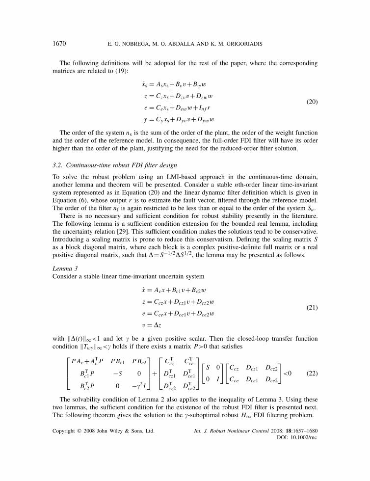
The following definitions will be adopted for the rest of the paper, where the correspondingmatrices are related to (19):

xs = Asxs+Bvv+Bww

z = Czxs+Dzvv+Dzww

e = Cexs+Deww+ In f r

y = Cyxs+Dyvv+Dyww

(20)

The order of the system ns is the sum of the order of the plant, the order of the weight functionand the order of the reference model. In consequence, the full-order FDI filter will have its orderhigher than the order of the plant, justifying the need for the reduced-order filter solution.

3.2. Continuous-time robust FDI filter design

To solve the robust problem using an LMI-based approach in the continuous-time domain,another lemma and theorem will be presented. Consider a stable nth-order linear time-invariantsystem represented as in Equation (20) and the linear dynamic filter definition which is given inEquation (6), whose output r is to estimate the fault vector, filtered through the reference model.The order of the filter nf is again restricted to be less than or equal to the order of the system Su .

There is no necessary and sufficient condition for robust stability presently in the literature.The following lemma is a sufficient condition extension for the bounded real lemma, includingthe uncertainty relation [29]. This sufficient condition makes the solutions tend to be conservative.Introducing a scaling matrix is prone to reduce this conservatism. Defining the scaling matrix Sas a block diagonal matrix, where each block is a complex positive-definite full matrix or a realpositive diagonal matrix, such that �= S−1/2�S1/2, the lemma may be presented as follows.

Lemma 3Consider a stable linear time-invariant uncertain system

x = Acx+Bc1v+Bc2w

z = Cczx+Dcz1v+Dcz2w

e = Ccex+Dce1v+Dce2w

v = �z

(21)

with ‖�(t)‖∞<1 and let � be a given positive scalar. Then the closed-loop transfer functioncondition ‖Twy‖∞<� holds if there exists a matrix P>0 that satisfies⎡

⎢⎢⎣PAc+AT

c P PBc1 PBc2

BTc1P −S 0

BTc2P 0 −�2 I

⎤⎥⎥⎦+

⎡⎢⎢⎣

CTcz CT

ce

DTcz1 DT

ce1

DTcz2 DT

ce2

⎤⎥⎥⎦[S 0

0 I

][Ccz Dcz1 Dcz2

Cce Dce1 Dce2

]<0 (22)

The solvability condition of Lemma 2 also applies to the inequality of Lemma 3. Using thesetwo lemmas, the sufficient condition for the existence of the robust FDI filter is presented next.The following theorem gives the solution to the �-suboptimal robust H∞ FDI filtering problem.



Theorem 4There exists an nth-order filter F to solve the �-suboptimal H∞ FDI filtering problem if there existmatrices X and Y with Y�X>0 such that the following conditions are satisfied:[

AsX+X ATs +�2BvS

−1BTv +BwBT

w XCTz +�2BvS

−1DTzv +BwDT

zw

CzX+�2DzvS−1BT

v +DzwBTw �2(DzvS

−1DTzv −S−1)+DzwDT

zw

]<0 (23)

⎡⎢⎢⎣

CTy

DTyv

DTyw

⎤⎥⎥⎦

⊥⎡⎢⎢⎣Y As+AT

s Y +CTz SCz+CT

e Ce Y Bv +CTz SDzv Y Bw +CT

z SDzw +CTe Dew

BTv Y +DT

zvSCz DTzvSDzv −S DT

zvSDzw

BTwY +DT

zwSCz+DTewCe DT

zwSDzv DTzwSDzw +DT

ewDew −�2 I

⎤⎥⎥⎦

×

⎡⎢⎢⎣

CTy

DTyv

DTyw

⎤⎥⎥⎦

⊥T

<0 (24)

[Y �I

�I X

]� 0

rank(X−Y ) � nf

(25)

The proof of this theorem is presented in Appendix B.

Conditions (23) and (24) of Theorem 3 are convex LMI constraints on the matrix parameters Xand Y . For the full-order FDI filtering problem, where nf=ns, the rank constraint (25) is redundantand the computational problem is a convex LMI problem. To find the parameterization of all robustfilters, Theorem 2 may be applied again, but it is necessary to find the new matrices. Consideringthe new state vector as a combination of the plant and filter states, xT=[xTs xTf ], the closed-loopsystem Fl(S,F), from the LFT scheme of Figure 6, is described by the following state-spaceequations:

x =[

As 0

BfCy Af

]x+

[Bv

BfDyv

]v+

[Bw

BfDyw

]w

z = [Cz 0]x+Dzvv+Dzww

e = [Ce+DfCy Cf]x+(DfDyv)v+(Dew +DfDyw)w

Adopting the formulation

x = (A0+BFM)x+(B01+BFE1)v+(B02+BFE2)w

z =C1x+D011v+D012w

e = (C2+H2FM)x+(H2FE1)v+(D022+H2FE2)w



the new introduced matrices are given by

A0 =[As 0

0 0

], B01=

[Bv

0

], B02=

[Bw

0

]

D011 = Dzv, D012=Dzw, D022=Dew

C1 = [Cz 0], C2=[Ce 0]

B =[0 0

0 I

], M=

[Cy 0

0 I

], E1=

[Dyv

0

], E2=

[Dyw

0

], H2=[I 0]

(26)

with the unknown filter defined as

F=[Df Cf

Bf Af

]

Applying Lemma 3, inequality (22) becomes

⎡⎢⎢⎣P(A+BFM)+(A+BFM)TP P(B01+BFE1) P(B02+BFE2)

(B01+BFE1)TP −S 0

(B02+BFE2)TP 0 −�2 I

⎤⎥⎥⎦

+

⎡⎢⎢⎣

CT1 (C2+H2FM)T

DT011 (H2FE1)

T

DT012 (D022+H2FE2)

T

⎤⎥⎥⎦[S 0

0 I

][C1 D011 D012

C2+H2FM H2FE1 D022+H2FE2

]<0

(27)

Applying Schur formula to (27), and using Lemma 2, it can be devised from (9) that

�=

⎡⎢⎢⎢⎢⎢⎢⎢⎣

PB

0

0

0

H2

⎤⎥⎥⎥⎥⎥⎥⎥⎦

, �=[M E1 E2 0 0] and �=

⎡⎢⎢⎢⎢⎢⎢⎢⎢⎣

PA+ATP PB01 PB02 CT1 CT

2

BT01P −S 0 DT

011 0

BT02P 0 −�2 I DT

012 DT022

C1 D011 D012 −S−1 0

C2 0 D022 0 −I

⎤⎥⎥⎥⎥⎥⎥⎥⎥⎦

(28)

Using the new �, � and � as defined by (28), Theorem 2 may now be applied to find theparameterization of all robust filters. For the reduced-order problem, the alternating projectionsmethod presented in the previous section (nominal case) may be applied.



Some comments are necessary to explain the use of the scaling matrix in Theorem 4 in theproposed algorithm. This scaling matrix is an attempt to reduce the conservatism of the robustsolutions that result from the general representation of the uncertainties and the non-existence ofa necessary and sufficient theorem for the robust case. But its inclusion results in a non-convexoptimization problem corresponding to inequalities (23)–(25) depending on the representationadopted. Recall that in Theorem 4 the scaling matrix S and also its inverse are present. To addressthis non-convex problem, an iterative solution is adopted, beginning with an initial value for thescaling matrix and after solving the LMIs of Theorem 4 in terms of X and Y and finding a filter,optimizing the cost � with respect to the S matrix. This procedure is repeated till an acceptablesolution is found. The proposed iterative algorithm is guaranteed to converge, but convergence to aglobal optimum for the � value is not guaranteed. The scaling matrix is similar to constant D-scalesfrom complex structured singular value theory [33] and the iterative approach corresponds to theD–K iteration for structured value synthesis [34].

4. NUMERICAL EXAMPLES

The proposed method is applied to a simulated example in this section. Consider a second-ordermechanical system that consists of a mass, spring and damper system, with parameter uncertainties(�1 and �2) in the stiffness and damping coefficients, respectively. The system is described by thefollowing state-space equations:

x1 = x2

x2 = −a0x1−a1x2+u+d+ f −v1−v2

z1 = �1a0x1

z2 = �2a1x2

y = (b0−b2a0)x1+(b1−b2a1)x2+b2u+b2d+b2 f −b2v1−b2v2

where a0=1,a1=1,b0=1,b1=0.3,b2=0.1. Assume that both the weight function and the refer-ence model are a second-order low-pass filter with two poles at −3rad/s, chosen in order to achievenoise rejection without affecting the plant dynamics in the low-frequency range. The uncertaintiesare 10% for �1 and 40% for �2.

Considering first the plant without weight functions and reference model, the nominal optimalvalue for the performance index � was found to be 0.7071 and for the robust case 0.8483. Ingeneral, it must be expected that the nominal index should be less than the robust index.

To analyze the performance of these systems, the uncertain model is simulated using the twodifferently designed filters. The singular value plots of the error transfer functions, i.e. the transfermatrix between the disturbance input and the filtering errors, are presented in Figure 7, for bothcases. These graphs were obtained using the nominal and robust filters and the plant being subjectedto five pairs of stiffness and damping coefficient uncertainties, respectively (2,8%), (4,16%),(6,24%), (8,32%) and (10,40%). This scheme of variation in uncertainties is followed in allgraphs presented here. For the nominal design, the horizontal line in the bottom corresponds tothe � optimal value in decibels. All the plots are above this value, implying that the performance



Frequency (rad/sec)

Sin

gula

r V

alue

s (d

B)

Singular Values

10-1

100

101

-3

-2.9

-2.8

-2.7

-2.6

-2.5

Nom

inal

Filt

er

Frequency (rad/sec)

Sin

gula

r V

alue

s (d

B)

Singular Values

10-1

100

101

-2.2

-2

-1.8

-1.6

Rob

ust

Filt

er

Figure 7. Nominal (above) and robust (below) FDI filter design results.

when the design does not take into account the uncertainty is indeed unbounded. For the robustdesign, the � value in decibels for the uncertain case now appears consistently in the top of thegraph, representing the limit for the singular value plots. However, it may be seen that the nominaldesign curves are below the respective robust curve, showing a better performance for the givenconstant uncertainties. This is an apparent contradiction, found also in the other presented designs.It may be explained based on the difference in the � value for the two designs and on the smallsensitivity of the used plant related to the uncertainties. The robust design is necessarily conserva-tive, and the scaling matrix is introduced in order to reduce this factor, but the proposed iterativeapproach cannot guarantee the optimal global solution. However, the lack of an upper bound forthe nominal design renders it unreliable, unless an accurate mathematical model of the plant isknown.

In Figure 8, the filter designs including the disturbance weight function are presented. Thenominal � value is the same 0.7071 and the robust one is 0.8432, just a little less than the valuefound before. However, it may be seen that the performance of both the designs are better thanin the previous cases, but some of the nominal curves still cross the horizontal bound line. Thisconfirms that the nominal design does not present a reliable upper limit. Again, the robust plotsare always below the optimal � value. The main difference, seen in both designs, is the low-passcharacteristic in all curves, caused by the introduction of the weight function.

Considering the inclusion of the reference model for the nominal and robust designs, therespective singular value plots may be seen in Figure 9. The � values are, respectively, 0.7071and 0.8477. The nominal design curves present the low-pass filter effect, but the high-frequency



Frequency (rad/sec)

Sin

gula

r V

alue

s (d

B)

Singular Values

10-1

100

101

-8

-7

-6

-5

-4

-3

Nom

inal

Filt

er

Frequency (rad/sec)

Sin

gula

r V

alue

s (d

B)

Singular Values

10-1

100

101

-4

-3.5

-3

-2.5

-2

-1.5

Rob

ust

Filt

er

Figure 8. Nominal and robust FDI filter design results, including the disturbance weight function.

rejection is better now compared with the design with the weighting function. Again, some curvesare above the respective � value in the low-frequency region. For the robust case, the results aresimilar to the previous cases. All curves are below the limit, but the high continuous roll-off inthe high-frequency region implies a better noise rejection.

5. CONCLUSIONS

An H∞ filter design for FDI, based on the estimation of the input fault vector, was presented for thenominal and the uncertain representation of the plant, using an LMI-based approach. Two differentsets of LMIs were obtained for each case, whose solution, if the problem is feasible, representsthe parameterization of all H∞ FDI filters. For the full-order problem, the filter design constraintsare convex, but for the reduced-order filter, an additional rank constraint results in a non-convexproblem. An alternating projections algorithm for this case was presented. The robust filteringformulation includes a scaling matrix to reduce the conservatism of this design. For this case, aniterative algorithm is proposed that alternates between the solution of the filter and the scalingparameters, but no global optimum convergence of the algorithm is guaranteed. The formulationswere used in a numerical simulated example with several different configurations showing thatincluding a reference model to filter the fault signals improves the performance. However, evenincluding the scaling matrix, the results for the examples are still conservative. The comparison



Frequency (rad/sec)

Sin

gula

r Val

ues

(dB

)

Singular Values

10-1

100

101

-20

-15

-10

-5

Nom

inal

Filt

er

Frequency (rad/sec)

Sin

gula

r V

alue

s (d

B)

Singular Values

10-1

100

101

-20

-15

-10

-5

Rob

ust

Filt

er

Figure 9. Nominal and robust FDI filter design results, including the reference model.

between the nominal and robust design results, for all examined cases, demonstrates the necessityof the robust design to guarantee a reliable upper bound of the error transfer functions.

APPENDIX A

A.1. Proof of Theorem 1

Considering the closed-loop system Fl(S,F) from the LFT scheme of Figure 3, and the definitionsin (15) and (16), and that the orthogonal complement of � is

�⊥ =

⎡⎢⎢⎣[B

H

]⊥0

0 I

⎤⎥⎥⎦⎡⎢⎢⎣P−1 0 0

0 0 I

0 I 0

⎤⎥⎥⎦

and defining

�=[B

H

]⊥=[I 0 0], �=

[A0P

−1+P−1AT0 0

0 −I

]and �=

[B0

D0

]



condition (10) of Lemma 2 leads to the inequality

��T+ 1

�2��T�T<0

Partitioning P as

P−1=[

Z Z12

ZT12 Z22

]

making X = Z−1, and substituting for the LFT matrices in (15), it yields the following inequality:

X As+ATs X+ 1

�2XBwBT

wX<0

which corresponds to condition (12) of Theorem 1.For condition (11) of Lemma 2, considering that

�T⊥ =

⎡⎢⎢⎣[MT

ET

]⊥0

0 I

⎤⎥⎥⎦

and the following definitions

=[MT

ET

]⊥, �=

[PA0+AT

0 P PB0

BT0 P −�2 I

]and �=[0 D0]

it can be easily shown that it becomes

�T+�T�T<0

Substituting, it yields[MT

ET

]⊥([PA0+AT

0 P PB0

BT0 P −�2 I

]+[

0

DT0

][0 D0]

)[MT

ET

]⊥T

<0

Partitioning P as

P=[

Y Y12

Y T12 Y22

]

and considering that

=[MT

ET

]⊥=⎡⎣[ CT

y

DTyw

]⊥0

⎤⎦⎡⎢⎣I 0 0

0 0 I

0 I 0

⎤⎥⎦

inequality (13) results after some simple algebraic manipulations.



APPENDIX B

B.1. Proof of Theorem 4

Considering the closed-loop system Fl(Su,F), from the LFT scheme of Figure 6, the definitionsin (27) and (28), and that

�⊥ =

⎡⎢⎢⎢⎢⎢⎢⎢⎢⎣

⎡⎢⎣

B

0

H2

⎤⎥⎦

⊥

0 0

0 I 0

0 0 I

⎤⎥⎥⎥⎥⎥⎥⎥⎥⎦

⎡⎢⎢⎢⎢⎢⎢⎢⎣

P−1 0 0 0 0

0 0 0 I 0

0 0 0 0 I

0 I 0 0 0

0 0 I 0 0

⎤⎥⎥⎥⎥⎥⎥⎥⎦

and defining

� =⎡⎢⎣

B

0

H2

⎤⎥⎦

⊥

, �=

⎡⎢⎢⎣AP−1+P−1AT P−1CT

1 P−1CT2

C1P−1 −S−1 0

C1P−1 0 −I

⎤⎥⎥⎦

�1 =⎡⎢⎣

B01

D011

0

⎤⎥⎦ and �2=

⎡⎢⎣

B02

D012

D022

⎤⎥⎦

condition (10) of Lemma 2 yields the inequality⎡⎢⎢⎣

��T ��1 ��2

�T1�T −S 0

�T2�T 0 −�2 I

⎤⎥⎥⎦<0

Applying the Schur complement formula, it becomes

��T+��1S−1�T1�T+ 1

�2��2�

T2�T<0 (B1)

Partitioning P as P−1=(1/�2)[

XX12

XT12

X22

], substituting for the LFT matrices in (28), and considering

that

�=

⎡⎢⎢⎢⎢⎣0 0

0 I

0 0

I 0

⎤⎥⎥⎥⎥⎦

⊥

=[I 0 0 0

0 0 I 0

]

substitution of these terms in (B1) multiplied by �2 leads easily to condition (23) of Theorem 4.



For the second part of Theorem 3, considering that

�T⊥ =

⎡⎢⎢⎢⎢⎢⎢⎢⎢⎣

⎡⎢⎢⎣

M

ET1

ET2

⎤⎥⎥⎦

⊥

0 0

0 I 0

0 0 I

⎤⎥⎥⎥⎥⎥⎥⎥⎥⎦

and the definitions

=

⎡⎢⎢⎣

M

ET1

ET2

⎤⎥⎥⎦

⊥

, �=

⎡⎢⎢⎣PA+ATP PB01 PB02

BT01P −S 0

BT02P 0 −�2 I

⎤⎥⎥⎦

�1 = [C1 D011 D012] and �2=[C2 0 D022]it can be easily shown that condition (11) of Lemma 2 becomes⎡

⎢⎢⎣�T �T1 �T2

�1T −S−1 0

�2T 0 −I

⎤⎥⎥⎦<0

Applying the Schur complement formula, it leads to the following inequality:

�T+�T1 S�1T+�T2�2

T<0 (B2)

Partitioning P as P=[Y Y12

Y T12 Y22

]and substituting the respective matrices in (28), it leads to

inequality (24).

ACKNOWLEDGEMENTS

The first author is thankful to FAPESP in Brazil for the financial support during his sabbatical visit at theUniversity of Houston.

REFERENCES

1. Beard RV. Failure accommodation in linear systems through self-reorganisation. Ph.D. Dissertation, MIT,Cambridge, MA, 1971.

2. Jones HL. Failure detection in linear systems. Ph.D. Thesis, Department of Aeronautics and Astronautics, MIT,Cambridge, U.S.A., 1973.

3. Willsky AS. A survey of design methods for failure detection in dynamic systems. Automatica 1976; 12:601–611.4. Frank PM. Fault diagnosis in dynamic systems using analytic and knowledge-based redundancy—a survey and

some new results. Automatica 1990; 26:459–474.5. Patton RJ. Robust model-based fault diagnosis: the state of the art. IFAC, Espoo, Finland, 1994; 1–24.6. Frank PM, Ding X. Survey of robust residual generation and evaluation methods in observer-based fault detection

systems. Journal of Process Control 1997; 7(6):403–424.7. Patton RJ, Frank PM, Clark RN (eds). Fault Diagnosis in Dynamic Systems: Theory and Applications. Prentice-

Hall: Englewood Cliffs, NJ, 1989.



8. Chen J, Patton RJ. Robust Model-based Fault Diagnosis for Dynamic Systems. Kluwer Academic Publishers:Boston, U.S.A., 1999.

9. Qiu Z, Gertler J. Robust FDI systems and H∞ optimization. Proceedings of the 32nd IEEE Conference onDecision and Control, San Antonio, U.S.A., 1993; 1710–1715.

10. Frank PM, Ding X. Frequency domain approach to optimally robust residual generation and evaluation formodel-based fault diagnosis. Automatica 1994; 30(5):589–804.

11. Douglas RK, Speyer JL. Robust fault detection filter design. Journal of Guidance, Control and Dynamics 1996;19(1):214–218.

12. Edelmayer A, Bokor J, Keviczky L. Robust detection filter design for linear systems: comparison of twoapproaches. Proceedings of 13th IFAC World Congress, 7f-01(6), San Francisco, CA, U.S.A., 1996; 37–42.

13. Chen J, Patton RJ. H∞ formulation and solution for robust fault diagnosis. Proceedings of the 14th IFAC WorldCongress, Beijing, China, 1999; 127–132.

14. Duan GR, Howe D, Patton RJ. Robust fault detection in descriptor linear systems via generalised unknown inputobservers. Proceedings of the 14th IFAC World Congress, Beijing, China, 1999; 43–48.

15. Hou M, Patton RJ. An LMI approach to H−/H∞ fault detection observers. UKACC International Conferenceon Control. IEE: London, 1996; 305–310. Conference Publication No. 427.

16. Rambeaux F, Hamelin F, Sauter D. Robust residual generation via LMI. Proceedings of the 14th World Congressof IFAC, Beijing, China, 1999; 241–246.

17. Hamelin F, Sauter D. Robust fault detection in uncertain dynamic systems. Automatica 2000; 36:1747–1754.18. Casavola A, Famularo D, Franze G. Robust fault detection of uncertain linear systems via quasi-LMIs. ACC,

Portland, Oregon, 2005; 1654–1659.19. Frisk E, Nielsen L. Robust residual generation for diagnosis including a reference model for residual behavior.

Automatica 2006; 42:437–445.20. Khosrowjerdi MJ, Nikhoukhah R, Safari-Shad N. Fault detection in a mixed H2/H∞ setting. IEEE Transactions

on Automatic Control 2005; 50:1063–1068.21. Zhong M, Ding SX, Bingyong T, Jeinsch T, Sader M. An LMI approach to design robust fault detection observers.

Fourth WCICA, Shanghai, China, 2002; 2705–2709.22. Henry D, Zolghadri A. Design of fault diagnosis filters: a multi-objective approach. Journal of Franklin Institute

2005; 342:421–446.23. Frisk E, Nielsen L. Robust residual generation for diagnosis including a reference model for residual behaviour.

Proceedings of 14th World Congress of IFAC, Beijing, China, 1999; 55–60.24. Zhong M, Ding SX, Lam J, Wang H. An LMI approach to design robust fault detection filter for uncertain LTI

systems. Automatica 2003; 39:543–550.25. Niemann HH, Stoustrup J. Filter design for failure detection and isolation in the presence of modelling errors and

disturbances. Proceedings of the 35th IEEE Conference on Decision and Control, Kobe, Japan, 1996; 1155–1160.26. Grigoriadis KM, Watson Jr JT. Reduced-order H∞ and L2–L∞ filtering via linear matrix inequalities. IEEE

Transactions on Aerospace and Electronic Systems 1997; 33(4).27. Watson Jr JT, Grigoriadis KM. Optimal unbiased filtering via linear matrix inequalities. Systems and Control

Letters 1998; 35:111–118.28. Li H, Fu M. A linear matrix inequality approach to robust H∞ filtering. IEEE Transactions on Signal Processing

1997; 45(9):2338–2350.29. Skelton RE, Iwasaki T, Grigoriadis KM. A Unified Algebraic Approach to Linear Control Design. Taylor &

Francis: London, 1998.30. Grigoriadis KM, Skelton R. Low order control design for LMI problems using alternating projections. Proceedings

of the 33rd IEEE Conference on Decision and Control, Orlando, U.S.A., 1996.31. Grigoriadis KM, Beran E. Alternating projection methods for LMI problems with rank constraints. In Recent

Advances in Linear Matrix Inequality Approach to Control, Niculescu S-I, El Ghaoui L (eds). SIAM: Philadelphia,PA, 1999.

32. Nobrega EG, Abdalla MO, Grigoriadis KM. A reference model LMI approach to fault detection and isolation.Proceedings of the IASTED International Conference on Intelligent Systems and Control 2000, Honolulu, U.S.A.,2000; 327–377.

33. Haddad WM, Collins Jr EG, Moser R. Structured singular value controller synthesis using constant D-scaleswithout D–K iterations. International Journal of Control 1996; 63(4):813–830.

34. Packard A, Doyle JC. The complex structured singular value. Automatica 1993; 29:71–109.


Robustfaultestimationofuncertainsystemsusing anLMI ...mece2hv/Papers/t_pdf5.pdf · DOI:...

Documents

Transcript of Robustfaultestimationofuncertainsystemsusing anLMI ...mece2hv/Papers/t_pdf5.pdf · DOI:...