Robust visual tracking via e cient manifold ranking with ... fileaInstitute of Image Processing and...
31
Robust visual tracking via efficient manifold ranking with low-dimensional compressive features Tao Zhou a , Xiangjian He b , Kai Xie a , Keren Fu a , Junhao Zhang a , Jie Yang a,* a Institute of Image Processing and Pattern Recognition, Shanghai Jiao Tong University, China b Faculty of Engineering and Information Technology, University of Technology, Sydney, Australia Abstract In this paper, a novel and robust tracking method based on efficient manifold ranking is proposed. For tracking, tracked results are taken as labeled nodes while candidate samples are taken as unlabeled nodes. The goal of tracking is to search the unlabeled sample that is the most relevant to the existing labeled nodes. Therefore, visual tracking is regarded as a ranking problem in which the relevance between an object appearance model and candidate samples is pre- dicted by the manifold ranking algorithm. Due to the outstanding ability of the manifold ranking algorithm in discovering the underlying geometrical structure of a given image database, our tracker is more robust to overcome tracking drift. Meanwhile, we adopt non-adaptive random projections to preserve the structure of original image space, and a very sparse measurement matrix is used to effi- ciently extract low-dimensional compressive features for object representation. Furthermore, spatial context is used to improve the robustness to appearance variations. Experimental results on some challenging video sequences show the proposed algorithm outperforms seven state-of-the-art methods in terms of ac- curacy and robustness. Keywords: Visual tracking; Appearance model; Manifold ranking; Random projections; Low-dimensional compressive features; Spatial context * Corresponding author. Tel. +86 21 3420 4033 Email address: [email protected] (Jie Yang) Preprint submitted to Pattern recognition November 28, 2014
Transcript of Robust visual tracking via e cient manifold ranking with ... fileaInstitute of Image Processing and...

Robust visual tracking via efficient manifold rankingwith low-dimensional compressive features
Tao Zhoua, Xiangjian Heb, Kai Xiea, Keren Fua, Junhao Zhanga, Jie Yanga,∗
aInstitute of Image Processing and Pattern Recognition, Shanghai Jiao Tong University,China
bFaculty of Engineering and Information Technology, University of Technology, Sydney,Australia
Abstract
In this paper, a novel and robust tracking method based on efficient manifold
ranking is proposed. For tracking, tracked results are taken as labeled nodes
while candidate samples are taken as unlabeled nodes. The goal of tracking is
to search the unlabeled sample that is the most relevant to the existing labeled
nodes. Therefore, visual tracking is regarded as a ranking problem in which the
relevance between an object appearance model and candidate samples is pre-
dicted by the manifold ranking algorithm. Due to the outstanding ability of the
manifold ranking algorithm in discovering the underlying geometrical structure
of a given image database, our tracker is more robust to overcome tracking drift.
Meanwhile, we adopt non-adaptive random projections to preserve the structure
of original image space, and a very sparse measurement matrix is used to effi-
ciently extract low-dimensional compressive features for object representation.
Furthermore, spatial context is used to improve the robustness to appearance
variations. Experimental results on some challenging video sequences show the
proposed algorithm outperforms seven state-of-the-art methods in terms of ac-
curacy and robustness.
Keywords: Visual tracking; Appearance model; Manifold ranking; Random
projections; Low-dimensional compressive features; Spatial context
∗Corresponding author. Tel. +86 21 3420 4033Email address: [email protected] (Jie Yang)
Preprint submitted to Pattern recognition November 28, 2014

1. Introduction
Visual tracking is a long standing research topic due to its wide range of ap-
plications such as behavior analysis, activity recognition, video surveillance, and
human-computer interaction [1, 2]. Although it has had a significant progress
in the past decades, developing an efficient and robust tracking algorithm is still5
a challenging problem due to numerous factors such as partial occlusion, illumi-
nation variation, pose change, abrupt motion, and background clutter. These
factors can lead to wrong association, and result in drift and even failure in
tracking.
The main tracking algorithms can be categorized two classes: generative10
[3, 4, 5, 6] and discriminative methods [7, 8, 9, 10, 11, 12, 13].
Generative methods focus on searching for the regions which are the most
similar to the tracked targets with minimal reconstruction errors of tracking.
Adaptive models including the WSL tracker [3] and IVT method [14] have been
proposed to handle appearance variation. Recently, sparse representation meth-15
ods have been used to represent an object by a set of trivial target templates
and trivial templates [6, 15] to deal with partial occlusion, pose variation and so
on. Therefore, it is critical to construct an effective appearance model in order
to handle various challenging factors. Furthermore, generative methods discard
useful information surrounding target regions that can be exploited to better20
separate objects from backgrounds.
Discriminative methods treat tracking as a classification problem that dis-
tinguishes the tracked targets from the surrounding backgrounds. A tracking
technique called tracking by detection has been shown to have promising results
in real-time. This approach trains a discriminative classifier online to separate25
an object from its background. Collins et al. [7] selected discriminative fea-
tures online to improve the tracking performance. Boosting method has been
used for object tracking through combining weak classifiers to establish a strong
classifier to select discriminative features, and some online boosting feature s-
election methods have been proposed for object tracking [8, 16]. Babenko et30
2

al. [9]proposed a novel online MIL algorithm for object tracking that achieves
superior results with real-time performance. An efficient tracking algorithm
based on compressive sensing theories was proposed by Zhang et al. [10]. It
uses low dimensional features randomly extracted from high dimensional multi-
scale image features in the foreground and background, and it achieves better35
tracking performance than other methods in terms of robustness and speed.
Moreover, although some efficient feature extraction techniques have been pro-
posed for visual tracking [8, 10, 12], there often exist a large number of samples
from which features need to be extracted for classification, thereby entailing
computationally expensive operations [9].40
The above tracking methods have shown promising performance. However,
they have some shortcomings. Firstly, although the goal of a generative method
is to learn an object appearance model, an effective searching algorithm and
measuring method to match candidate samples to an object model are difficult
to obtain. Secondly, background varies broadly during a tracking process, so45
it is difficult to achieve the aim of a discriminative method to distinguish a
target region from a complicated background when the target looks similar
to its background. Therefore, it is very difficult to construct a discriminative
object representation. Thirdly, feature selection is of crucial importance for
generating an effective appearance model. However, approaches using a large50
amount of features make the computational load very heavy. Therefore, the
computational complexity of tracking methods is rather high, , and this limit
the real-time applications of these methods.
Graph-based ranking algorithms have been widely applied to information
retrieval and have proved to have excellent performance and feasibility on a va-55
riety of data types [17, 18, 19]. The manifold ranking algorithm first constructs
a weighted graph by considering each data node as a vertex. The ranking score
of the query is iteratively propagated to nearby node via the weighted graph.
Finally nodes will be ranked according to the ranking scores, in which a larger
score indicates higher relevance. In this paper, we develop a novel and robust60
tracking method based on manifold ranking, which regards tracking as a rank-
3

ing problem. As shown in Figure 1, we mark the tracked results as labeled
nodes, while candidate samples are regarded as unlabeled nodes. The track-
ing objective is to estimate the corresponding likelihood that is determined by
the relevance between the queries and all candidate samples. We use a mani-65
fold structure to measure the relevance between a model and samples, and in
our method low-dimensional compressive features can efficiently compress fea-
tures of foreground objects and their background. Experimental results on some
challenging video sequences are demonstrated to show the effectiveness and ro-
bustness of the proposed model and algorithm in comparison with seven state-of70
the-art tracking methods.
The main contributions of this paper are as follows.
1. A novel visual tracking method based on graph-manifold ranking is pro-
posed.
2. An efficient manifold ranking algorithm is adopted, it can reconstruct75
graph efficiently in each tracking round and reduce the computation com-
plexity.
3. Low-dimensional compressive features of an image are extracted by a very
sparse measurement matrix for object representation. This matrix pre-
serves the structure of the image and discriminates objects from their80
cluttered background effectively.
4. Our method exploits both temporal and spatial context information, and
it is robust to appearance variations caused by abrupt motion, occlusion
and background clutters.
5. Experimental results show that the proposed algorithm outperforms seven85
state-of-the-art methods in terms of accuracy and robustness.
This is is an extension of our paper showing preliminary results in [20]. The
rest of this paper is organized as follows. Graph-manifold ranking algorithm is
described in Section 2.1. Details of our proposed method based on an efficient
manifold ranking with low-dimensional compressive features are demonstrated90
in Section 3. The efficient manifold ranking algorithm is described in Section
4

2.2. Experimental results are shown and analyzed in Section 4. The conclusion
is presented in Section 5.
2. Preliminaries
2.1. Graph-based manifold ranking95
Manifold Ranking (MR), a graph-based ranking algorithm, has been widely
applied in information retrieval and shown to have excellent performance and
feasibility on a variety of data types [17, 18]. The manifold ranking method
is described as follows: given a query node, the remaining unlabeled nodes are
ranked based on their relevance to the given query. The goal is to learn a ranking100
function to define the relevance between unlabeled nodes and this query [18, 19].
In [19, 21], a ranking method that exploits the intrinsic manifold structure
of data for graph labelling is proposed. Given a data set X = {x1, x2, · · · , xn} ∈<m×n, where m is the dimension of feature vector and n is the number of the
data set, some data points are labelled queries and the rest need to be ranked105
according to their relevance to the queries. Let f : X → <n denote a ranking
function which assigns a ranking value ri to each point xi, and r is a column
vector defined by r = [r1, r2, · · · , rn]T . Let y = [y1, y2, · · · , yn]T denote an
indication vector, in which yi = 1 if xi is a query, and yi = 0 otherwise. Suppose
all data points represent a graph G = (V,E), where V represents vertex set,110
and edges E are weighted by an affinity matrix W = [wij ]n×n. The strength of
edge reflects the similarity between two vertices. To find the optimal ranking of
queries, the cost function associated with r is defined as follows.
O(r) =1
2(
n∑i,j=1
‖ 1√Dii
ri −1√Djj
rj‖2 + µn∑
i=1
‖ri − rj‖2) (1)
where µ > 0 controls the balance of the smoothness constraint (the first term)115
and the fitting constraint (the second term), D is a diagonal matrix with the
element Dii =∑nj=1 wij , for i, j = 1, 2, · · · , N . To minimize the cost function,
we can obtain the closed form solution as:
r∗ = (I − αS)−1y (2)
5

where I is an identity matrix, α = 11+µ and S = D− 1
2WD− 12 . Then, we use the
iteration scheme to solve the following optimal problem:120
r(t+ 1) = αS(r(t) + (1− α)y) (3)
where α is control parameter, which balances each points information from its
neighbors and and the original information.
2.2. Efficient manifold ranking algorithm
In order to efficiently reconstruct graph, we use efficient manifold ranking
algorithm [19] to compute the ranking score. First, we briefly introduce how to125
use anchor graph to model the data. Given a data set X = {x1, x2, · · · , xn} ∈
<m×n, U = {u1, u2, · · · , ud} ∈ <m×d indicates a set of anchors sharing the same
space with the data set. Then, we define a real value function r : X → R, which
assigns a semantic label for each point in X. The aim is to find a weight matrix
that measures relevance between data points r : X → R and anchors in U . We130
obtain r(x) for each point by a weighted average of these labels on anchors as
follows:
r(xi) =
d∑k=1
zkir(uk), i = 1, 2, · · · , n (4)
where∑dk=1 zki = 1 and zki > 0, in which zki represents the weight between
point xi and an anchor uk. The weights can be obtained by Nadaraya-Watson
kernel regression to increase smoothness. The graph construction process and135
the means to get the anchors can be found in detailed [19].
We use a new approach to represent the adjacency matrix W . The weight
matrix Z ∈ <d∗n can be viewed as a d-dimensional representation of the data
X ∈ <m∗n, in which d is the number of anchor points. It means that data points
can be presented in a new space to replace the original feature space. We set140
the adjacency matrix as follows:
W = ZTZ (5)
6

where Wij > 0 if two points are correlative and they will share at least one
common anchor point, otherwise Wij = 0. The new adjacency matrix is useful
to explore relevance among data points. According to W = ZTZ, equation (2)
can be rewritten as follows:145
r∗ = (T1 − αHTH)−1y = (I1 −HT (HHT − 1
αI2)−1H)y (6)
where H = ZD−1 and S = HTH, I1 and I2 are the identity matrices. By
equation(6), the inversion computation part have changed form a matrix n× n
to a matrix d×d. Therefore, the change can efficiently reduce computation load
for d� n. We can also note that the matrix D is computed without using the
adjacency matrix W . In equation (6),150
Dii =
n∑j=1
wij =
n∑j=1
zTi zj = zTi v (7)
where zi is the ith column of Z, and v =∑nj=1 zj . Thus, we compute the matrix
D without using the adjacency matrix W . By the equation (6), we multiply a
matrix to avoid the matrix - matrix multiplication every time. Therefore, the
efficient manifold ranking algorithm has a complexity O(dn+ d3). Due to a low
complexity for computing the ranking function r∗, we can reconstruct graph in155
each tracking round efficiently.
2.3. Low-dimensional compressive features
The Haar-like features have been widely used for object representation and
appearance modeling. They are typically designed for different tasks such as
object detection, object tracking and et al. [9, 10, 22]. However, Harr-like fea-160
tures require high computational loads for feature extraction in training and
tracking phases. Recently, Babenko et al. [9] adopted the generalized Haar-like
features where each one is a linear combination of randomly generated rectan-
gle features, and used online boosting to select a small set of them for object
tracking. In our tracking framework, we use the low-dimensional compressive165
features proposed by Zhang et al. [10] for the appearance modelling. A large
7
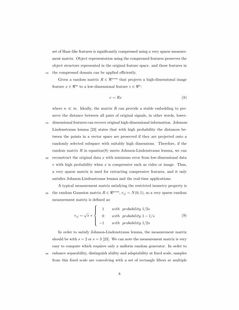
set of Haar-like features is significantly compressed using a very sparse measure-
ment matrix. Object representation using the compressed features preserves the
object structure represented in the original feature space. and these features in
the compressed domain can be applied efficiently.170
Given a random matrix R ∈ <n∗m that projects a high-dimensional image
feature x ∈ <m to a low-dimensional feature v ∈ <n:
v = Rx (8)
where n � m. Ideally, the matrix R can provide a stable embedding to pre-
serve the distance between all pairs of original signals, in other words, lower-
dimensional features can recover original high-dimensional information. Johnson-175
Lindenstrauss lemma [23] states that with high probability the distances be-
tween the points in a vector space are preserved if they are projected onto a
randomly selected subspace with suitably high dimensions. Therefore, if the
random matrix R in equation(8) meets Johnson-Lindenstrauss lemma, we can
reconstruct the original data x with minimum error from low-dimensional data180
v with high probability when x is compressive such as video or image. Thus,
a very sparse matrix is used for extracting compressive features, and it only
satisfies Johnson-Lindenstrauss lemma and the real-time applications.
A typical measurement matrix satisfying the restricted isometry property is
the random Gaussion matrix R ∈ <n∗m, rij ∼ N(0, 1), so a very sparse random185
measurement matrix is defined as:
rij =√s×
1 with probability 1/2s
0 with probability 1− 1/s
−1 with probability 1/2s
(9)
In order to satisfy Johnson-Lindenstrauss lemma, the measurement matrix
should be with s = 2 or s = 3 [23]. We can note the measurement matrix is very
easy to compute which requires only a uniform random generator. In order to
enhance separability, distinguish ability and adaptability at fixed scale, samples190
from this fixed scale are convolving with a set of rectangle filters at multiple
8

scales. Each rectangular filter at a scale is defined
hp,q(x, y) =
1 1 ≤ x ≤ p, 1 ≤ y ≤ q
0 otherwise(10)
where (xi, yi) is the coordinates of the upper left corner in the rectangular
filter, p and q are the width and height of the rectangle filter respectively.
Convolving an image patch with the rectangle filter at a fixed scale is equivalent195
to computing the internal image characters corresponding to this filter. Finally,
we represent each filtered image as a column vector in <wh and then concatenate
these vectors as a very high-dimensional multi-scale image feature vector x.
Then, a very sparse matrix is adopted to project x onto a low-dimensional
feature vector v. In tracking process, the sparse matrix remains fixed in whole200
tracking process and it is computed once in the original stage. Therefore, a
low-dimensional compressive features v can be efficiently computed and it is
used to represent an object.
3. Our proposed method
3.1. Framework205
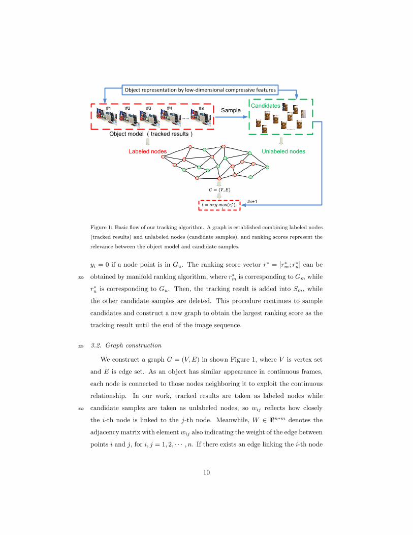
Figure 1 shows the basic flow of our proposed tracking algorithm. The
tracking problem is formulated as a ranking task. Firstly, we assume the lo-
cations in the first t frames have been obtained by CT tracker [10]. Let l(x∗i )
denote the location of tracking result at the i-th frame where x∗i represents
the sample. Then, we collect these tracked results to form the object appear-210
ance model set Sm = {x∗1, x∗2, · · · , x∗i }, i = 1, 2, · · · , t, and the corresponding
graph is taken as Gm. Secondly, for a new frame, we crop out a set of im-
age patches xr with N samples near the location l(x∗t ) with a search radius
at the current frame, i.e. xβ = {x : ‖l(x) − l(x∗t )‖ < β}. These candidate
image patches are collected to form a set of unlabeled nodes, represented by,215
Su = {xs+11 , xs+1
2 , · · · , xs+1i }, i = 1, 2, · · · , N , and the corresponding graph is
taken as Gu. Thirdly, the candidate Gu is combined with Gm to construct a
graph G = Gm ∪ Gu, in which the label yi = 1 if a node point is in Gm, and
9
……
#1 #2 #3
Object model (tracked results)
#s
……
Labeled nodes Unlabeled nodes
Sample
#s+1
Object representation by low-dimensional compressive features
𝐺 = (𝑉,𝐸)
𝑖 = 𝑎𝑟𝑔max𝑖(𝑟𝑢
∗)𝑖
#4Candidates
Figure 1: Basic flow of our tracking algorithm. A graph is established combining labeled nodes
(tracked results) and unlabeled nodes (candidate samples), and ranking scores represent the
relevance between the object model and candidate samples.
yi = 0 if a node point is in Gu. The ranking score vector r∗ = [r∗m; r∗u] can be
obtained by manifold ranking algorithm, where r∗m is corresponding to Gm while220
r∗u is corresponding to Gu. Then, the tracking result is added into Sm, while
the other candidate samples are deleted. This procedure continues to sample
candidates and construct a new graph to obtain the largest ranking score as the
tracking result until the end of the image sequence.
3.2. Graph construction225
We construct a graph G = (V,E) in shown Figure 1, where V is vertex set
and E is edge set. As an object has similar appearance in continuous frames,
each node is connected to those nodes neighboring it to exploit the continuous
relationship. In our work, tracked results are taken as labeled nodes while
candidate samples are taken as unlabeled nodes, so wij reflects how closely230
the i-th node is linked to the j-th node. Meanwhile, W ∈ <n∗m denotes the
adjacency matrix with element wij also indicating the weight of the edge between
points i and j, for i, j = 1, 2, · · · , n. If there exists an edge linking the i-th node
10
and the j-th node, the weight between the two nodes can be defined by
wij = e−||ci−cj ||
2
2σ2 (11)
where ci and cj denote the feature representation for two nodes in the feature235
space respectively, σ is a constant that controls the strength of the weight. By
ranking all nodes on the construction graph, we can obtain a nonzero relevance
value for any nodes on the graph.
3.3. Appearance model updating process
As shown in Figure 1, we can obtain the locations in the first t frames by240
a CT tracker, and then to obtain the location of the t + 1 frame by manifold
ranking algorithm. There exists an obvious problem that the size of Sm will
be very large if all tracked results are added into the appearance model in each
tracking round, so the computation complexity will be very heavy. In addition,
the bad node impacts the performance of the appearance model. To track the245
next frame, we need to update the appearance model firstly. We compute the
average ranking score of r∗m;
µr∗m =
t∑i=1
(r∗m)i (12)
where (r∗m)i represents the score of the i-th node in Sm. Then, we compute
the displacement error ei between the score of each node in Sm and the average
score:250
ei = ‖(r∗m)i − µr∗m‖2 (13)
We delete the node that has the largest displacement error, and then add
the current tracking result x∗t+1 into Sm. Thus, the number of Sm will be t
constantly. It is worth noting that the average ranking score computed from
tracked results alleviates the noise effects.
11

Algorithm 1. The proposed tracking method
Input: Video frame f=1:F
1. The first t frames are tracked by a CT tracker to
construct an object appearance model set
Sm = {x∗1, x∗2, · · · , x∗i }
2. for f= t+1 to F do
3. Crop out a set of candidate samples as unlabeled set
Su by xβ = {x : ‖l(x)− lt(x∗))‖ < β}.
4. if f == t+1
5. Construct a graph G = Gm ∪Gu and support set Ss.
6. Update model set Sm.
7. else
8. Construct a graph G = Gm ∪Gs ∪Gu.
9. Update model set Sm and support set Ss.
10. end if
11. The i-th candidate sample that has the largest in all ru
is taken as the object location, the i-th sample can be
selected by i = argmaxi r∗u, i = 1, 2, · · · , U , where U is
the number of candidate samples.
12. end for
Output: Tracking results {l1(x∗), l2(x∗), · · · , lF (x∗)}.
255
3.4. Support set construction
In our method, object appearance model Sm only reflects the temporal re-
lationship among consecutive frames, while it can not consider its immediate
surrounding background. In the tracking process, the context of a target in an
image sequence consists of the spatial context including the local background260
and the temporal context including all appearances of the targets in the previous
frames. As shown in Figure 2 (left), our object appearance model Sm repre-
12

……
#1 #2 #3
Appearance model
(temporal relationship)
#s
Spatial relationship
Figure 2: Temporal and spatial relationship.
sents the temporal context in the previous frames. In Figure 2 (right), note that
the object can be influenced by its surrounding background, and there exists a
correlation between the object (denoted by red rectangle) and its surrounding265
background (denoted by yellow rectangle). Therefore, in order to make use of
surrounding background information and provide much appearance information
for graph construct, we establish a support set to describe the spatial context.
The spatial context describes the relevance between the object and its surround-
ing background in small neighborhood region.270
Supposed that, in tracking the (t+ 1)-th frame, we have obtained the object
location l(x∗t+1) with ranking score, and the ranking score of the current candi-
date samples is denoted by r∗u. We select s nodes from the candidate samples set
Su to construct the support set Ss. Ss is corresponding to the first s+ 1 largest
ranking scores among all obtained r∗u, and we then delete the largest one. The275
graph corresponding to the support set is denoted by Gs. The updating process
of the appearance model and the construction of the support set construction
are shown in Figure 4.
To track the (t+ 2)-th frame, a graph G = Gm ∪Gs ∪Gu is constructed and
the label yi = 1 if a node point is from Sm and Ss, while yi = 0 if a node point280
is from Su. The ranking score matrix r∗ = [r∗m; r∗s ; r∗u] can be obtained by an
efficient manifold ranking algorithm (see Section.2.2), where r∗m, r∗s , and r∗u are
13

Tracked results
Model nodes set Unlabeled nodes set
Current samplesSupport nodes set
𝒓∗ Compute
𝒓𝒖∗
Samples from the previous candidates with larger ranking score
Update set
Update set
𝑺𝒎
𝑺𝒎
𝑺𝒔
𝑺𝒔
𝑺𝒖
𝒊 = 𝒂𝒓𝒈𝐦𝐚𝐱𝒊(𝒓𝒖
∗ )𝒊
Construct graph
Figure 3: The updating process of appearance model and the construction of support set.
(a) Lemming (b) Coke (c) DavidOutdoor
(e) Stone (f) Couple(d) Deer (g) Bolt
Figure 4: The caption of tracking different object in video sequences.
14

Table 1: Evaluated video sequences.
Sequences #Frames Challenging Factors
Deer 71 abrupt motion, background clutter
Coke 291 abrupt motion, partial occlusion
Bolt 293 partial occlusion, scale change
Stone 593 partial occlusion, background clutter
Couple 140 partial occlusion, abrupt motion, background clutter
Lemming 1336 partial occlusion, abrupt motion, background clutter
DavidIndoor 252 partial occlusion, illumination variation
corresponding to Gm, Gs, Gu respectively. The tracking scheme is summarized
in Algorithm 1. Finally, the target in frame t+ 2 is the sample with the largest
component in r∗u, as the i-th sample can be selected from Su and computed by285
i = argmaxi
r∗u, i = 1, 2, · · · , U (14)
where U is the number of candidate samples.
4. Experimental results and analysis
4.1. Experimental setup
We evaluate the proposed tracking method based on an efficient manifold
ranking algorithm and an object representation with low-dimensional features290
using seven video sequences with impacted factors including abrupt motion,
cluttered background, severe occlusion and appearance change (See Table 1).
We compare our proposed tracker with seven other state-of-the-art methods
including: L1 tracker (L1) [6], real-time compressive tracking (CT) [10], multi-
ple instance learning tracker (MIL) [9], incremental visual tracking (IVT) [14],295
fragment tracker (Frag) [4], weighted multiple instance learning tracker (WMIL)
[24] and locally orderless tracking (LOT) [25]. For fair comparison, we adopt
the source or binary codes provided by the authors with tuned parameters for
best performance. But for some trackers involving randomness, we repeat the
experimental results 5 times on each sequence and obtain the averaged results.300
15

Table 2: Center location error (CLE). Red fonts indicate the best performance while the blue
fonts indicate the second best ones.
Sequence L1 CT MIL IVT Frag WMIL LOT Ours
Coke 85.3 42.0 26.9 70.5 124.8 76.9 42.5 23.9
Bolt 39.4 211.4 35.8 138.8 18.8 214.3 68.2 7.6
Deer 171.5 95.1 66.5 127.5 92.1 25.1 65.9 23.0
Stone 19.2 32.8 32.3 2.5 65.9 99.8 28.1 6.4
Couple 110.6 33.8 33.9 105.1 32.6 34.4 37.8 9.3
Lemming 184.9 26.3 25.9 93.4 149.1 96.9 19.9 24.3
DavidOutdoor 100.4 87.3 38.4 52.9 90.5 73.3 63.5 29.5
Average CLE 101.6 75.5 37.1 84.4 81.9 88.7 46.6 17.7
In our experiments, the parameters are used in our algorithm as follows.
The search radius for cropping out candidate samples is set to β = 20, which
is related with object motion speed. The dimensionality of the compressive
feature is set to 200. The first t frames are tracked by the CT method and t is
set to 30. The number of nodes in support set is set s = 10. Implemented in305
MATLAB, our tracking method runs at about 10 frames per second (FPS) to
obtain the averaged results on an i3 3.20 GHz machine with 4 GB RAM.
4.2. Quantitative analysis
We perform experiments on seven publicly available standard video sequences.
As the ground truth, the center position of a target in a sequence is labeled310
manually. This ground truth is provided in Wu’s work [26]. For quantitative
analysis, we use average center location errors as evaluation criteria to compare
the performance, and the pixel error in every frame is defined as follow:
CLE =√
(x′ − x)2 + (y′ − y)2 (15)
where (x′, y′) represents the object position obtained by different tracking meth-
ods, and (x, y) is the ground truth. The second evaluated metric is the success315
16

Table 3: Success rate (SR)(%). Red fonts indicate the best performance while the blue fonts
indicate the second best ones.
Sequence L1 CT MIL IVT Frag WMIL LOT Ours
Coke 13.1 50.2 72.2 15.8 3.5 44.8 13.7 79.4
Bolt 27.5 4.7 44.4 3.4 54.6 3.1 17.4 81.7
Deer 3.9 14.1 21.3 11.7 7.6 83.5 35.2 85.9
Stone 29.2 35.2 32.1 65.2 15.4 8.4 27.8 65.2
Couple 12.3 67.8 71.4 10.1 64.3 65.3 69.7 92.8
Lemming 3.9 74.8 53.5 17.8 13.4 24.4 84.5 82.1
DavidOutdoor 27.5 22.4 64.8 41.1 19.5 29.8 31.2 72.3
Average SR 16.8 38.5 51.4 23.9 25.5 37.1 40.0 79.9
rate [27], and the score in every frame is defined as follow:
score =area(ROIT ∩ROIG)
area(ROIT ∪ROIG)(16)
where ROIT is the tracking bounding box and ROIG is the ground truth bound-
ing box. If the score is larger than 0.5 in one frame, the tracking result is con-
sidered as a success. Table 2 reports the center location error, where smaller
CLE means more accurate tracking results. In Table 2, each row represents the320
average center location errors of the eight algorithms testing on a certain video
sequence. The number marked with red indicates the best performance in a
certain testing squence, and blue indicates the second best. Table 3 reports the
success rates, where larger average scores mean more accurate results. From
Table 2 and Table 3, we can see that our method achieves the best or second325
best performance compared with L1, CT, MIL, WMIL, Frag, IVT and LOT for
most of sequences. Moreover, we draw the error curve according to equation
(15) for each video sequences (Figure 5). In addition, Figure 6, Figure 7 and
Figure 8 show the screen captures for some of the video clips. More details of
experiments are analyzed and discussed in the following subsections.330
17

0 50 100 150 200 250 3000
50
100
150
200
250
300
350
Frame Number
Lo
ca
tio
n E
rro
r(p
ixe
l)
Bolt
0 50 100 150 200 250 3000
50
100
150
200
250
300
Frame Number
Lo
ca
tio
n E
rro
r(p
ixe
l)
Coke
0 20 40 60 80 100 120 1400
50
100
150
200
250
Frame Number
Lo
ca
tio
n E
rro
r(p
ixe
l)
Couple
0 10 20 30 40 50 60 70 800
50
100
150
200
250
300
Frame Number
Lo
ca
tio
n E
rro
r(p
ixe
l)
Deer
0 20 40 60 80 100 1200
20
40
60
80
100
120
140
160
180
200
Frame Number
Lo
ca
tio
n E
rro
r(p
ixe
l)
Stone
0 50 100 150 200 250 3000
50
100
150
200
250
300
350
400
450
Frame Number
Lo
ca
tio
n E
rro
r(p
ixe
l)
DavidOutdoor
0 50 100 150 200 2500
50
100
150
200
250
300
350
400
450
Frame Number
Lo
ca
tio
n E
rro
r(p
ixe
l)
Lemming
Figure 5: Error plots of all tested sequences for different tracking methods.18

#55#55#101#223#262#55 #55#55#101#223#262#55#101 #55#55#101#223#262#55#101#223 #55#55#101#223#262#55#101#223#262
#55#55#101#223#262#55#101#223#262#313 #55#55#101#223#262#55#101#223#262#313#426 #55#55#101#223#262#55#101#223#262#313#426#495 #55#55#101#223#262#55#101#223#262#313#426#495#535
#49#49 #49#49#158 #49#49#158#279 #49#49#158#279#487
#49#49#158#279#487#550 #49#49#158#279#487#550#1096 #49#49#158#279#487#550#1096#1105 #49#49#158#279#487#550#1096#1105#1126
(a) Stone
(b) Lemming
L1 CT MIL IVT Frag WMIL LOT Ours
Figure 6: Sampled tracking results for tested sequences of (a) Stone and (b) Lemming.
19

4.3. Qualitative analysis
Partial occlusion: The objects suffer heavy or longtime partial occlusion,
scale change, deformation and rotation in sequences Bolt(Figure 8(a)), Lem-
ming (Figure 7(b)), DavidOutdoor(Figure 6(c)), Coke (Figure 6(a))). In the
Bolt sequence, Figure 8(a) demonstrate that our tracking method performs well335
in terms of position and scale when the objects undergo severe occlusion and
deformation at frames #112, #157, #167, while the other methods including
the IVT, CT, WMIL and L1 completely fail to track the objects in these frames.
This can be attributed to some reasons: (1) we can extract discriminative fea-
tures by a very sparse matrix to separate an object well from its background,340
and also object representation with low-dimensional compressive features can
preserve the structure of original image space; and (2) the outstanding ability of
manifold ranking algorithm is to discover the underlying geometrical structure
and the relevance between object appearance and candidate samples. Thus,
our tracker is more robust to overcome tracking drift and abrupt motion. In345
the DavidOutdoor sequence, our method and MIL perform better than other
methods at frames #193, #206 and #252. The other methods suffer from sev-
er drift and some of these methods completely fail to track. Furthermore, our
method performs more accurately than MIL at frames #230 and #252. Thus,
our method can handle occlusion and it is not sensitive to partial occlusion since350
the manifold ranking algorithm can measure the relevance between object ap-
pearance and candidate samples. Furthermore, we can also see the advantages
of our tracking method in Lemming and Coke sequences (see Figure 7(b) and
Figure 6(a)).
Abrupt motion and blur: The objects in Deer (Figure 8(b)), Coke (Fig-355
ure 6(a))), Couple (Figure 6(b)) and Lemming (Figure 7(b)) sequences have
abrupt motions. It is difficult to predict the location of a tracked object when
it undergoes an abrupt motion. As illustrated in Figure 8(b), when an object
undergoes an in-plane rotation, all evaluated algorithms except the proposed
tracker do not track the object well. We also see that the WMIL method can360
track the object well except in frames #43 and #56. The CT method suffers
20

(b) Couple
(c) Davidoutdoor
(a) Coke
#51 #134 #143
#173 #226 #247
#122
#203
#17 #55 #55#84 #55#84#95
#55#84#95#103 #55#84#95#103#109 #55#84#95#103#109#117 #55#84#95#103#109#117#135
L1 CT MIL IVT Frag WMIL LOT Ours
#26#26 #26#26#68#177#26#26#68#177#92 #26#26#68#177#92#193
#26#26#68#177#92#193#206 #26#26#68#177#92#193#206#214 #26#26#68#177#92#193#206#214#230 #26#26#68#177#92#193#206#214#230#252
Figure 7: Sampled tracking results for tested sequences of (a) Coke, (b) Couple and (c)
DavidOutdoor.
21

completely from drifts to the background at frames #7, #17, #39, #43, #56,
#60 and #68. In the Coke sequence, we can see that our method perform bet-
ter than other all evaluated algorithms (see all shown frames in Figure 7(a)).
For the Couple sequence, our tracker performs better than the other methods365
whereas the WMIL, LOT,and MIL algorithms are able to track the objects in
some frames. In the Lemming sequence, only the CT and our method perform
well at frame #550, while the other algorithms fail to track the target object-
s well. What is more, the Frag method suffers completely from drift in the
shown frames, which verifies that the Frag method cannot adaptively adjust370
these changes, resulting in serious drifts. We can also see that the LOT method
can track the object well except that there are few drifts in a couple of frames
see frames #550 and #1105). Blurry images exist in the Deer sequence (see
Figure 8(b)), because a fast motion make it difficult to track the target object.
As shown in frames #56 and #71 of Figure 8(a), our proposed method can still375
track the object well compared with other methods.
Background clutters: The trackers are easily confused an object is very
similar to its background. Figure 8(b), Figure 6(b), Figure 7(b) and Figure
7(a) demonstrate the tracking results in the Deer, Couple, Lemming and Stone
sequences with background clutters. Figure 7(a) shows different trackers track380
a yellow cobblestone located among a lot of similar stones. Thus, it is very
difficult to distinguish the object from its background and to keep tracking
the object correctly. Comparatively, our method and the IVT exhibit better
discriminative ability and outperform other methods at frames #495 and #535.
The MIL and WMIL trackers completely drift to the background at frames385
#426, #495 and #535, which verifies that the selected features by the MIL
and WMIL trackers are less informative than our method. The Frag tracker has
severe drifts at all frames except frames #55 and #535 because its template does
not update online, making it unable to handle large background clutter. The
CT method has severe drifts at frames #426, #495 and #535 because it only390
uses compressive features and the Bayesian classifier is sensitive to background
clutter.
22
#112 #157 #167 #167#178
#167#178#185#191 #167#178#185#191#209 #237 #255
#7#7 #7#7#17 #7#7#17#39 #43
#43#56 #60 #68 #68#71
(a) Bolt
(b) Deer
L1 CT MIL IVT Frag WMIL LOT Ours
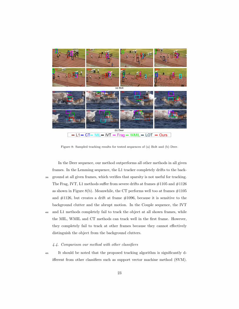
Figure 8: Sampled tracking results for tested sequences of (a) Bolt and (b) Deer.
In the Deer sequence, our method outperforms all other methods in all given
frames. In the Lemming sequence, the L1 tracker completely drifts to the back-
ground at all given frames, which verifies that sparsity is not useful for tracking.395
The Frag, IVT, L1 methods suffer from severe drifts at frames #1105 and #1126
as shown in Figure 8(b). Meanwhile, the CT performs well too at frames #1105
and #1126, but creates a drift at frame #1096, because it is sensitive to the
background clutter and the abrupt motion. In the Couple sequence, the IVT
and L1 methods completely fail to track the object at all shown frames, while400
the MIL, WMIL and CT methods can track well in the first frame. However,
they completely fail to track at other frames because they cannot effectively
distinguish the object from the background clutters.
4.4. Comparison our method with other classifiers
It should be noted that the proposed tracking algorithm is significantly d-405
ifferent from other classifiers such as support vector machine method (SVM).
23

……
#1 #2 #3 #s
Positive samples Negative samples
Negative samplesPositive samples
(1) SVM(a)
(2) SVM(b)
Figure 9: Two sampling methods using SVM classifier. (1) The tracked results are selected
as positive samples, while many image patches are selected away from the current location
as negative samples; (2) These image patches around the current location are collected as
positive samples, while many image patches are selected away from the current location as
negative samples
24

#82 #110 #192
#100 #130 #200
#101 #251 #401
(a) Bolt
(b) DavidOutdoor
(c) Lemming
SVM(a) SVM(b) Ours
Figure 10: Comparison our tracking method with SVM classifiers.
The outstanding ability of of the manifold learning algorithm is to discover the
underlying geometrical structure and the relevance between different data set,
while SVM. To verify the performance of our tracker outperforms the perfor-
mance of using SVM classifier, We construct the two tracking methods using410
SVM. In Figure 9(1), we assume the locations in the first t frames have been
obtained by CT tracker [10], then these tracked results are selected as positive
samples, while many image patches are selected away from the current loca-
tion as negative samples (See Figure 9(1) for details). In Figure 9(2), we collect
these image patches around the current location as positive samples, while many415
image patches are selected away from the current location as negative samples.
In these experiments, we use the Haar feature to represent the object and
the dimensionality of the compressive feature is set to 200. The first t frames
25

Table 4: Center location error (CLE) for comparing our method with SVM classifiers.
Methods Deer Stone Coke Bolt Couple Lemming DavidOutdoor
SVM(a) 97.1 82.4 56.5 81.8 33.4 162.1 68.7
SVM(b) 60.2 68.9 86.1 33.4 18.9 165.6 67.9
Ours 23.0 6.4 23.9 7.6 9.3 24.3 29.5
are tracked by the CT method and t is set to 30. Table 4 reports the center
location error, where smaller CLE means more accurate tracking results. From420
Table 4, we can see that our method achieves the best performance compared
with SVM classifiers. Figure 10 show the screen captures for some of the video
clips. In Bolt sequence, we can see the two SVM methods completely fail to
track the target object in the frames #200 and there are some tracking error in
frames #130 and #130. In DavidOutdoor and Lemming sequences, our tracker425
performs better than the other methods.
4.5. Discussion
As shown in our experiments, our method can address these factors including
abrupt motion, cluttered background, occlusion more effectively. The reason-
s are as follows. (1) We can extract discriminative features by a very sparse430
matrix to separate an object well from its background, and the object repre-
sentation with low-dimensional compressive features can preserve the structure
of original image space. (2) The outstanding ability of of the manifold ranking
algorithm is to discover the underlying geometrical structure and the relevance
between object appearance and candidate samples. (3) Our method combines435
temporal with spatial context information for tracking, and it is very insensitive
to multiple factors. Thus, our tracker can obtain favorable performance.
However, our proposed method may fail when an out-of-plane rotation and
an abrupt motion occur in the current sequence (see Figure 11). Figure 11(a)
shows an out-of-plane rotation and an abrupt motion after #75. Our method440
drifts away the ground truth because the appearance model can not match well
26

#60 #75 #75#90
#260 #260#290 #260#290#320
(a)
(b)
Figure 11: Two failed tracking cases:(a) out of plane rotation and abrupt motion; (b) similar
appearance information between object and non-objects.
between the object model and the candidates, and it cannot distinguish the
object from the changed background. However, our method is sensitive when
there exists a complex background and when there exists similar appearance in-
formation between the object and the non-objects in a sequence (Figure 11(b)).445
Therefore, our method can not distinguish an object from background clutter-
s. Overall, our method performs favorably against the other state-of-the-art
tracking methods in the challenge sequences.
5. Conclusions
This paper has proposed a novel framework named manifold ranking based450
visual tracking. The algorithm is initially proposed to rank data along their
manifold, which has been widely applied in information retrieval and shown to
have excellent performance and feasibility on a variety of data types. In order to
address the shortcomings of original manifold ranking from graph reconstruction
and heavy computation load, we adopt the efficient manifold ranking algorithm.455
The ability for efficiently constructing a graph is more applicable for tracking
problem. What is more, we adopt non-adaptive random projections to preserve
the structure of original image space, and a very sparse measurement matrix has
27

been used to efficiently extract compressive features for object representation.
Furthermore, our method exploits temporal and spatial context information460
for tracking, which is very insensitive to background clutters and appearance
change. Experiments on some challenging video sequences have demonstrated
the superiority of our proposed method to seven state-of-the-art ones in accuracy
and robustness.
Acknowledgments465
This research is partly supported by NSFC, China (No: 61273258, 61105001),
and Ph.D. Programs Foundation of Ministry of Education of China (No.20120073110018).
References
[1] A. Yilmaz, O. Javed, M. Shah, Object tracking: A survey, Acm computing
surveys (CSUR) 38 (4) (2006) 13.470
[2] W. Hu, T. Tan, L. Wang, S. Maybank, A survey on visual surveillance
of object motion and behaviors, Systems, Man, and Cybernetics, Part C:
Applications and Reviews, IEEE Transactions on 34 (3) (2004) 334–352.
[3] A. D. Jepson, D. J. Fleet, T. F. El-Maraghi, Robust online appearance mod-
els for visual tracking, Pattern Analysis and Machine Intelligence, IEEE475
Transactions on 25 (10) (2003) 1296–1311.
[4] A. Adam, E. Rivlin, I. Shimshoni, Robust fragments-based tracking using
the integral histogram, in: Computer Vision and Pattern Recognition, 2006
IEEE Computer Society Conference on, Vol. 1, IEEE, 2006, pp. 798–805.
[5] J. Kwon, K. M. Lee, Visual tracking decomposition, in: Computer Vision480
and Pattern Recognition (CVPR), 2010 IEEE Conference on, IEEE, 2010,
pp. 1269–1276.
28

[6] X. Mei, H. Ling, Robust visual tracking using l1 minimization, in: Com-
puter Vision, 2009 IEEE 12th International Conference on, IEEE, 2009,
pp. 1436–1443.485
[7] R. T. Collins, Y. Liu, M. Leordeanu, Online selection of discriminative
tracking features, Pattern Analysis and Machine Intelligence, IEEE Trans-
actions on 27 (10) (2005) 1631–1643.
[8] H. Grabner, M. Grabner, H. Bischof, Real-time tracking via on-line boost-
ing., in: BMVC, Vol. 1, 2006, pp. 6–15.490
[9] B. Babenko, M.-H. Yang, S. Belongie, Robust object tracking with on-
line multiple instance learning, Pattern Analysis and Machine Intelligence,
IEEE Transactions on 33 (8) (2011) 1619–1632.
[10] K. Zhang, L. Zhang, M.-H. Yang, Real-time compressive tracking, in: Com-
puter Vision–ECCV 2012, Springer, 2012, pp. 864–877.495
[11] Z. Kalal, J. Matas, K. Mikolajczyk, Pn learning: Bootstrapping binary clas-
sifiers by structural constraints, in: Computer Vision and Pattern Recog-
nition (CVPR), 2010 IEEE Conference on, IEEE, 2010, pp. 49–56.
[12] K. Zhang, H. Song, Real-time visual tracking via online weighted multiple
instance learning, Pattern Recognition 46 (1) (2013) 397–411.500
[13] K. Fu, C. Gong, Y. Qiao, J. Yang, I. Y.-H. Gu, One-class support vec-
tor machine-assisted robust tracking, Journal of Electronic Imaging 22 (2)
(2013) 023002–023002.
[14] D. A. Ross, J. Lim, R.-S. Lin, M.-H. Yang, Incremental learning for robust
visual tracking, International Journal of Computer Vision 77 (1-3) (2008)505
125–141.
[15] T. Bai, Y. Li, Robust visual tracking with structured sparse representation
appearance model, Pattern Recognition 45 (6) (2012) 2390–2404.
29

[16] H. Grabner, C. Leistner, H. Bischof, Semi-supervised on-line boosting for
robust tracking, in: Computer Vision–ECCV 2008, Springer, 2008, pp.510
234–247.
[17] J. He, M. Li, H.-J. Zhang, H. Tong, C. Zhang, Manifold-ranking based
image retrieval, in: Proceedings of the 12th annual ACM international
conference on Multimedia, ACM, 2004, pp. 9–16.
[18] D. Zhou, J. Weston, A. Gretton, O. Bousquet, B. Scholkopf, Ranking on515
data manifolds., in: NIPS, Vol. 3, 2003.
[19] B. Xu, J. Bu, C. Chen, D. Cai, X. He, W. Liu, J. Luo, Efficient manifold
ranking for image retrieval, in: Proceedings of the 34th international ACM
SIGIR conference on Research and development in Information Retrieval,
ACM, 2011, pp. 525–534.520
[20] T. Zhou, X. He, K. Xe, K. Fu, J. Zhang, J. Yang, Visual tracking via graph-
based efficient manifold ranking with low-dimensional compressive features,
Multimedia and Expo (ICME), 2014 IEEE International Conference on,
IEEE, 2014 (Accepted).
[21] C. Yang, L. Zhang, H. Lu, X. Ruan, M.-H. Yang, Saliency detection via525
graph-based manifold ranking, in: Computer Vision and Pattern Recogni-
tion (CVPR), 2013 IEEE Conference on, IEEE, 2013, pp. 3166–3173.
[22] P. Viola, M. Jones, Rapid object detection using a boosted cascade of simple
features, in: Computer Vision and Pattern Recognition, 2001. CVPR 2001.
Proceedings of the 2001 IEEE Computer Society Conference on, Vol. 1,530
IEEE, 2001, pp. 511–518.
[23] D. Achlioptas, Database-friendly random projections: Johnson-
lindenstrauss with binary coins, Journal of computer and System
Sciences 66 (4) (2003) 671–687.
[24] K. Zhang, H. Song, Real-time visual tracking via online weighted multiple535
instance learning, Pattern Recognition 46 (1) (2013) 397–411.
30
[25] S. Oron, A. Bar-Hillel, D. Levi, S. Avidan, Locally orderless tracking, in:
Computer Vision and Pattern Recognition (CVPR), 2012 IEEE Conference
on, IEEE, 2012, pp. 1940–1947.
[26] Y. Wu, J. Lim, M.-H. Yang, Online object tracking: A benchmark, in:540
Computer Vision and Pattern Recognition (CVPR), 2013 IEEE Conference
on, IEEE, 2013, pp. 2411–2418.
[27] M. Everingham, L. Van Gool, C. K. Williams, J. Winn, A. Zisserman,
The pascal visual object classes (voc) challenge, International journal of
computer vision 88 (2) (2010) 303–338.545
31


![Lighting Test Methods and Standards-Jiao[1]](https://static.fdocuments.in/doc/165x107/577cc4191a28aba711981fd1/lighting-test-methods-and-standards-jiao1.jpg)