
ROBUST SHAPE DESIGN TECHNIQUES FOR STEADY-STATE METAL FORMING
131
ROBUST SHAPE DESIGN TECHNIQUES FOR STEADY-STATE METAL FORMING PROCESSES A dissertation submitted in partial fulfillment of the requirements for the degree of Doctor of Philosophy By JALAJA REPALLE B.TECH., Kakatiya University, 2001 __________________________________________ 2006 Wright State University
Transcript of ROBUST SHAPE DESIGN TECHNIQUES FOR STEADY-STATE METAL FORMING

ROBUST SHAPE DESIGN TECHNIQUES
FOR STEADY-STATE METAL FORMING PROCESSES
A dissertation submitted in partial fulfillment of the
requirements for the degree of
Doctor of Philosophy
By
JALAJA REPALLE
B.TECH., Kakatiya University, 2001
__________________________________________
2006
Wright State University
WRIGHT STATE UNIVERSITY
SCHOOL OF GRADUATE STUDIES
September 5, 2006
I HEREBY RECOMMEND THAT THE DISSERTATION PREPARED UNDER MY
SUPERVISION BY Jalaja Repalle ENTITLED Robust Shape Design Techniques for
Steady-State Metal Forming Processes BE ACCEPTED IN PARTIAL FULFILLMENT
OF THE REQUIREMENTS FOR THE DEGREE OF Doctor of Philosophy.
Ramana V. Grandhi, Ph.D.
Dissertation Director
Ramana V. Grandhi, Ph.D.
Director, Ph.D. Program
Joseph F. Thomas, Jr., Ph.D.
Dean, School of Graduate Studies
Committee on Final Examination
Ramana V. Grandhi, Ph.D., WSU
Raghavan Srinivasan, Ph.D., WSU
Nathan Klingbeil, Ph.D., WSU
Rajiv Shivpuri, Ph.D., OSU
Jandro I. Abot, Ph.D., UC

iii
ABSTRACT
Repalle, Jalaja. Ph.D., Department of Mechanical and Materials Engineering, Wright
State University, 2006. Robust Shape Design Techniques for Steady-State Metal Forming
Processes.
Metal forming is a process that transforms a simple shape of a workpiece into
a predetermined complex shape through the application of compressive/tensile forces
exerted by dies. In the design of a forming process, the only factors that are known
are the final component shape and the material with which it is to be made. Then the
engineer has to design a process to make defect-free product, subject to limitations of
shape, material properties, cost, time, and other such factors. The design cycle can be
enhanced if performance sensitivity information is available that could be used with
any commercially available finite element software. Hence, this research investigates
the analytical continuum-based sensitivity analysis method using boundary integral
and material derivative formulations. Sensitivity derivation starts by obtaining an
identity integral for the non-linear deformation process. Then the adjoint problem is
introduced to obtain an explicit expression for the sensitivity of the objective and
constraint functions. The applicability of sensitivity analysis is demonstrated through
a steady-state metal forming process.
In conventional optimization all the parameters are considered as deterministic
and constant. However, in practice, they are prone to various uncertainties such as
variations in billet geometry, die temperature, material properties, workpiece and
forming equipment positional errors, and process parameters. A combination of these
uncertainties could induce heavy manufacturing losses through premature die failure,
final part geometric distortion, and production risk. Identifying, quantifying, and

iv
controlling the uncertainties will reduce risk in the manufacturing environment and
will minimize the overall cost of production. Hence, in this research, a robust design
methodology is developed by considering the randomness in the parameters. The
developed methodology is applied for die shape optimization of an axisymmetric
extrusion. Die angle and spline through points are the design variables; friction factor
and ram velocity are considered as random parameters. The optimization problem is
formulated to minimize the exit velocity variance by placing constraints on average
strain and variance. Further, the solutions of reliability-based optimization are
compared with deterministic-based optimization solutions. The results herein indicate
that the robust design solution gives better product quality and reduces the total exit
velocity variance.

v
TABLE OF CONTENTS
List of Figures ........................................................................................................viii
List of Tables............................................................................................................. x
1. Introduction...................................................................................................... 14
1.1. Motivation ................................................................................................ 14
1.2. Research Tasks ......................................................................................... 18
2. Literature Review ............................................................................................. 21
2.1. Non-Gradient-based Optimization Techniques .......................................... 21
2.2. Gradient-based Optimization Techniques .................................................. 22
2.2.1. Backward Optimization ..................................................................... 23
2.2.2. Forward Optimization........................................................................ 25
2.2.3. Discrete Approach ............................................................................. 26
2.2.4. Continuum Approach......................................................................... 28
2.2.5. Boundary Integral Approach.............................................................. 29
3. Deformation Mechanics.................................................................................... 31
3.1. Metal Forming Analysis............................................................................ 31
3.2. Material Properties.................................................................................... 32
3.3. Effective Strain and Effective Stress ......................................................... 33
3.4. Equilibrium Equations .............................................................................. 34
3.5. Plastic Potential Equation.......................................................................... 34
3.6. Virtual Work-Rate Principle...................................................................... 35
3.7. Boundary Conditions ................................................................................ 36
3.7.1. Velocity Boundary Conditions........................................................... 36

vi
3.7.2. Traction Boundary Conditions ........................................................... 36
3.7.3. Contact Boundary Conditions ............................................................ 37
3.8. Design Objectives ..................................................................................... 39
4. Design Sensitivity Analysis .............................................................................. 41
4.1. Continuum Sensitivity Analysis ................................................................ 43
4.1.1. Lagrangian Framework...................................................................... 44
4.1.2. Eulerian Framework .......................................................................... 45
4.2. Material Derivative Concepts.................................................................... 46
4.2.1. Material Derivative Definition........................................................... 46
4.2.2. Material Derivative of a Functional on Boundary .............................. 48
4.2.3. Material Derivative of s ..................................................................... 53
4.3. Sensitivity Derivation ............................................................................... 55
4.3.1. Identity Integral Formulation ............................................................. 57
4.3.2. Material Derivative on Identity Integral ............................................. 60
4.3.3. Material Derivative of Objective/Constraint Functional ..................... 64
4.3.4. Adjoint Problem Definition ............................................................... 67
4.3.5. Sensitivity Formulation ..................................................................... 68
4.4. Implementation ......................................................................................... 69
4.5. Case Study - Extrusion.............................................................................. 71
4.5.1. Process and Boundary Conditions...................................................... 72
4.5.2. Design Parameters and Shape Variation Vector ................................. 74
4.5.3. Objective/Constraint Functionals ....................................................... 75
4.5.4. Primal FEM Analysis ........................................................................ 76

vii
4.5.5. Computation of Adjoint Boundary Conditions ................................... 77
4.5.6. Calculation of Sensitivity Vector ....................................................... 80
5. Design Optimization......................................................................................... 90
5.1. Design of Experiments .............................................................................. 92
5.2. Improved Two-Point Adaptive Non-Linear Approximation....................... 93
5.3. Multi-Point Approximation ....................................................................... 95
5.4. Optimization Problem ............................................................................... 96
6. Robust Design ................................................................................................ 103
6.1. Possible Sources of Uncertainties............................................................ 105
6.2. Screening of Critical Parameters ............................................................. 107
6.3. Probability Distributions ......................................................................... 109
6.3.1. Normal Distribution......................................................................... 109
6.3.2. Standard Normal Distribution .......................................................... 110
6.3.3. Lognormal and Gamma Distributions .............................................. 111
6.3.4. Cumulative Distribution Function.................................................... 112
6.4. Response Variability ............................................................................... 112
6.5. Reliability Index ..................................................................................... 113
6.6. Reliability-Based Optimization ............................................................... 115
7. Summary ........................................................................................................ 120
8. Future Directions............................................................................................ 122
9. Bibliography................................................................................................... 124

viii
List of Figures
Fig 1. Closed Die Forging........................................................................................ 15
Fig 2. Tube Extrusion .............................................................................................. 15
Fig 3. Rod Drawing ................................................................................................. 15
Fig 4. Strip Rolling .................................................................................................. 16
Fig 5. General Boundary Value Problem Conditions ................................................ 31
Fig 6. Equilibrium of Surface Tractions ................................................................... 37
Fig 7. Schematic Diagram of Curved Die and Workpiece......................................... 39
Fig 8. General Shape Optimization Procedure.......................................................... 42
Fig 9. Lagrangian Description for Material Deformation.......................................... 44
Fig 10. Eulerian Description of Material Deformation ............................................. 45
Fig 11. Variation in Domain .................................................................................... 47
Fig 12. Material Derivative of An Arc Segment, Normal Component....................... 49
Fig 13. Material Derivative of An Arc Segment, Tangential Component.................. 50
Fig 14. Tangential Derivatives ................................................................................. 52
Fig 15. Material Derivative of s, Normal Component............................................... 53
Fig 16. Material Derivative of s, Tangential Component .......................................... 54
Fig 17. Continuum Sensitivity Analysis Approach ................................................... 56
Fig 18. Overall Procedure for Sensitivity Calculation .............................................. 70
Fig 19. Finite Element Model Extrusion - Boundary Conditions .............................. 72
Fig 20. Die Angle and Velocity Distribution ............................................................ 74
Fig 21. Strain Variance Sensitivities ........................................................................ 82
Fig 22. Average Strain Sensitivities ......................................................................... 83
ix
Fig 23. Exit Velocity Variance Sensitivities ............................................................. 83
Fig 24. Average Strain, Strain Variance, and Maximum Strains with Die Angle ...... 85
Fig 25. Maximum Von Mises Stress and Ram Force with Die Angle ....................... 85
Fig 26. Design Parameters (ri, zi) ............................................................................. 87
Fig 27. Shape Optimization Procedure with Function Approximations..................... 91
Fig 28. Central Composite Design ........................................................................... 93
Fig 29. Velocity Variance Actual vs. Approximation Values ................................... 98
Fig 30. Strain Variance - Actual vs. Approximation Values ..................................... 99
Fig 31. Average Strain - Actual vs. Approximation Values ...................................... 99
Fig 32. Design Variable Convergence History ....................................................... 100
Fig 33. Objective and Constraint Functions Convergence History.......................... 101
Fig 34. Robust Design Methodology...................................................................... 105
Fig 35. Interaction among State Variables and Uncertainty Sources ....................... 106
Fig 36. Pareto Plot Process Performance ................................................................ 108
Fig 37. Notmal Distribution ................................................................................... 110
Fig 38. Standard Normal Distribution .................................................................... 111
Fig 39. Normal CDF .............................................................................................. 112
Fig 40. Reliability Index ........................................................................................ 114
Fig 41. Design Variable Convergence .................................................................... 117
Fig 42. Objective and Constraint Functions Convergence ...................................... 117

x
List of Tables
Table 1. Strain Variance Sensitivities....................................................................... 80
Table 2. Average Strain Sensitivities ....................................................................... 81
Table 3. Exit Velocity Variance Sensitivities ........................................................... 81
Table 4. Process Responses with Die Angle ............................................................. 84
Table 5. Objective Functions Sensitivities for Different Design Parameters ............. 88
Table 6. TANA 2 Approximation Parameters........................................................... 97
Table 7. Optimum Points with Different Starting Points......................................... 116
Table 8. DBO and RBO Results ............................................................................. 118

xi
Acknowledgements
I am deeply thankful to my advisor Professor Ramana V. Grandhi for his
invaluable guidance, patience, and personal attention over the last several years. I will
always be grateful to him for bringing me to United States and providing me an
opportunity to become a part of his outstanding research group. His inspirational
debates, insightful suggestions, and continuous encouragement made me think
responsibly about my studies and career. The competitive spirit and expertise that he
provided will be a source for inspiration in my professional career and personal life.
I would like to take this opportunity to convey my gratitude to Professor Choi
for educating me on boundary sensitivity methods. I am also thankful to him for
providing continuous help in derivations and excellent feedback and suggestions,
without which I could not have finished my formulation and implementation
successfully.
I wish to express my sincere thanks to my Ph.D. committee members and my
colleagues at the Computational Design and Optimization Center at Wright State
University for providing valuable suggestions and comments and also for creating
friendly environment that often mitigated personal tensions and promoted my work
ability. I extend my very special thanks to Alysoun, whose English corrections and
suggestions significantly improved my writing style and language.
I would like to gratefully acknowledge the support from the National Institute
of Standards and Technology, Advanced Technology Program, under agreement
number 70NANB0H3014, and from the Ph.D. Assistantship granted by Wright State
University.

xii
I am so fortunate and proud to have such the unwavering support of my
parents, Sudhakara Swamy and Vakuladevi, and younger siblings, Jayakiran and
Jayanthi. They inspired and strengthened me emotionally, spiritually, and
intellectually in every step of my life. Their love and tolerance enabled me to pursue
my higher studies in the USA. I would like to remember my grandmother, Venkata
Ratnamma, for providing a strong base for my academic development.
I am deeply indebted to my fiancé, Srikanth Verma Regula, for his continuous
encouragement and support. His eternal trust and patient love raised my confidence in
my down times.
I would like to thank my companions Vani, Malini, Nag, and Virajitha for
their continuous friendship, belief, and encouragement. I also would like to remember
my dearest late friend Lavanya, who made me realize my ambitions and leaving an
unforgettable impression in my life.
I also extend my thanks to all of my roommates from the last four years for
being on my side in my good and bad times. I also would like to acknowledge all of
my friends and former mentors for their good wishes and advice, which helped me a
lot in finishing up my doctoral studies successfully.

xiii
Dedication To my parents and family

14
1. Introduction
1.1. Motivation
Many complex industrial and military components, as well as many consumer
goods, are produced through forming processes. Forming is a plastic deformation
process in which a simple cylindrical shape, either hot or cold, is transformed through
a number of stages to a predetermined shape, primarily by compressive forces exerted
by dies. Metal forming processes offer potential savings in energy and material—
especially in medium and large production quantities, where tool costs can be easily
amortized. In addition, parts produced by metal forming exhibit better mechanical and
metallurgical properties and reliability than do those manufactured by casting and
machining.
In general, metal forming processes can be classified as bulk forming
processes and sheet-metal forming processes [Kobayashi et al. (1989)]. In sheet-metal
forming processes, the workpiece is a sheet or a part fabricated from a sheet. The
deformation usually causes significant changes in shape, but not in cross section, of a
sheet. Whereas in bulk metal forming processes, the workpiece undergoes large
plastic deformation, resulting in an appreciable change in shape or cross section.
These processes include batch processes [Figs. 1-2] such as forging and extrusion,
and continuous processes [Figs. 3-4] such as drawing and rolling.

15
Fig 1. Closed Die Forging
Fig 2. Tube Extrusion
Fig 3. Rod Drawing
Upper die
Lower die
Flash
Flash land
Upper die
Lower die
Workpiece
Die force
Force
Die
Die bearing area
Force
Ejector pin
Workpiece
Die
Workpiece
Drawing
force

16
Fig 4. Strip Rolling
The starting billet shape for most of the forming operations is simple: a bar
with a round, square, or rectangular cross section. The goal of the forming designer is
to design the process equipment and conditions to obtain the final component from
these simple shapes by avoiding problems like fold over, excessive ram forces,
localized deformation, and geometric distortion. The main immediate goal is to obtain
defect free product with optimum material flow. The direction of material flow
determines both the mechanical properties related to local deformation and the
formation of defects, such as cracks or folds, at or below the surface. The local metal
flow is in turn influenced by
• Forming tool geometry
• Die-workpiece interface friction conditions
• Material flow stress and formability
• Thermal conditions existing in the deformation zone
• Complexity of the final shape
An accurate determination of the effects of these parameters on metal flow is a
prime requirement for proper design and control of any metal forming process.
Without knowledge of the influence of such variables as friction conditions, material
+
+
Roll
Roll
Workpiece

17
properties, and process geometry on the process mechanics, it would not be possible
to control the change of the metallurgical structure of the deforming material or to
predict and prevent the occurrence of defects [Lee et al. (1977)]. Today, sophisticated
finite element-based simulation packages are providing localized information of the
deformation process and assisting in the process optimization.
Process optimization includes the design of: die shapes, number of stages,
process parameters such as ram velocity, billet and die temperatures and lubrication
system. Among all conventional design problems, die shape optimization is
considered to be the most difficult because they deal with geometric data such as die
boundary shape as design variables, and the shape should be changed during the
optimization procedure. Additionally, material flow, defect formation, and
dimensional accuracy of the final product are directly related to the performance of
the dies, apart from other factors such as billet material, forming press and ancillary
equipment capability, and the later heat treatment operations [Arif et al. (2003)]. For
example, improper extrusion die shapes give rise to excessive hydrostatic tensile
stresses at the centerline of the deformation zone and lead to formation of internal
cracks such as center-bursts. And because of its high cost, based on special material
and processing, very strict dimension tolerances, and high demands on repeated
thermo-mechanical performance, the most critical extrusion component is perhaps the
die.
Generally, these die shapes are designed through extensive trial-and-error
methods. The die shapes obtained through the physical build-and-test approach are
adequate for delivering the final part, but may not be the optimal shapes for cost and

18
quality. In spite of having advanced simulation and design techniques, metal forming
process design still faces obstacles, such as long simulation times and the black box
nature of simulation tools. The development of analytical sensitivity analysis and
optimization techniques will allow metal forming simulations to be used more
intelligently. Sensitivity analysis provides quantitative measure of the effects of die
shapes, process conditions and other such factors on the process performance. They
provide the search direction, in which if the design is moved will lead to optimum
performance such as minimum material wastage, geometrical distortions, and forming
power. In addition, optimization techniques reduce the iteration trials, the total
manufacturing cost, and the product delivery time and improve tool life and product
quality.
Except at start and end, forming processes such as extrusion, rolling, and
drawing are steady-state. The shape design problem in steady-state processes is
characterized by large displacements and nonlinear material behavior. In addition, the
process performance affects by variations in process and operating conditions. These
variations often lead to unpredicted die failure modes and process break-downs.
Based on the characteristics and nature of the process, the following research tasks
were identified and performed.
1.2. Research Tasks
The main objectives of this research are the development and implementation
of efficient shape design methods for steady-state forming components in the
presence of uncertainties. To accomplish this goal, several primary tasks of this
research are identified as follows:

19
• Development of design strategies for steady-state metal forming processes
• Development of a design method that uses non-linear continuum plasticity
governing equations, which make the process robust and invariant to FEM
formulations
• Development of sensitivity analysis approaches that can best utilize the
analysis results from any available commercial FEM package
• Development of an analysis method to identify deterministic or
probabilistic components of the forming process
• Development of a reliability-based design methodology to optimize the
forming process in the presence of uncertain parameters
Generally speaking, two optimization schemes can be used to optimize the die
shapes. The first scheme is based on sensitivity information, and the other scheme
uses non-gradient approximation methods such as response surface method. The
sensitivity information can be obtained by using finite difference method; also it can
be obtained analytically. The use of later scheme is limited because it is
computationally expensive. In the former scheme, analytical sensitivities can be
computed either by utilizing finite element formulations or by continuum process
mechanics. All the commercial software packages are black box in nature. Therefore,
in this research, a new continuum process mechanics-based sensitivity analysis
technique is developed. The proposed method utilizes non-linear continuum equations
of the deformation process and material derivative concepts. The approach starts by
investigating deformation mechanics and formulating an identity integral for the
20
forming process. Adjoint variables method is employed to obtain an explicit boundary
integral formula for the sensitivities of objective and constraint functions.
Moreover, in a conventional design, all the parameters are considered as
deterministic and constant. However, in practice, forming processes are prone to
various uncertainties, such as variations in billet/workpiece geometry, lubrication
properties, material properties, workpiece and forming equipment positional errors
and process parameters. A combination of these uncertainties could induce heavy
manufacturing losses through premature die failure, final part geometric distortion
and production risk. Identifying the sources of uncertainties, and then quantifying and
controlling them, reduces risk in the manufacturing environment and minimizes the
overall cost of production. Hence, a novel robust design technique is developed to
account for uncertainties in the process. Uncertainty quantification and reliability-
based optimization are the two tools that are employed in robust design technique.
The effectiveness of the proposed methodologies is demonstrated with applications to
steady-state metal forming process. Further, the reliability-based design solutions are
compared with conventional design solutions. The results herein indicate that the
robust design solution improves the product quality and reduces the geometric
distortion.

21
2. Literature Review
Several gradient and non-gradient-based optimization techniques have been
developed to optimize die shapes in metal forming processes.
2.1. Non-Gradient-based Optimization Techniques
Some of the non-gradient methods for die shape optimization are using
knowledge-based systems, genetic algorithms, neural networks, fuzzy logic
techniques, and response surface methods. Chung et al. (1998) have done research in
the application of genetic algorithms for the design of material processes.
A genetic algorithm is a design technique that is based on the survival of the
fittest design in a population of designs. The design variable is represented as a binary
string. The optimal designs achieved after generations of population are useful when
one is concerned with the design of a single process where different objectives may
be required by the process engineer at various times. However, if the network has to
deal with the design of different processes (new situations require re-training), then
the method loses its merit.
Mehta et al. (1999) developed extrusion die design technique using neural
networks and design of experiments. Neural networks is an artificial intelligence
technique where the network is trained using input-output data of various simulations
of a process. Once trained, the neural network can be used for process design,
obviating the need for a simulation. Schenk et al. (2004) reported an evolutionary

22
automatic design technique for optimal design of metal forming die surfaces. The
computer-aided die surface shapes are eventually changed based on finite element
simulations.
The above mentioned evolutionary design methods are powerful techniques
that handle discrete design data with ease (e.g., number of stages in multi-stage
design). However, these methods are very inefficient compared to gradient-based
methods in the case of continuous design data, especially in systems where evaluation
of the objective function and constraints is costly. Convergence near the optimal
solution is also slow. Hence, there exists a natural bias towards accurate and efficient
gradient-based shape optimization techniques.
2.2. Gradient-based Optimization Techniques
In the gradient-based shape optimization problem, the most popular algorithm is
to use the gradient of the objective function and constraint values in search of an
optimum shape. When facing the shape optimization problem, the following choices must
be made:
• Which optimization technique should be used, forward or backward?
• How final sensitivities should be obtained, directly (Direct Differentiation
Method-DDM) or by basic independent variables (Adjoint Variable
Method-AVM)?
• When design differentiation should be carried out, before or after the finite
element discretization?
• How should one differentiate with respect to the shape variables (e.g.,
Control Volume Method-CVM and Material Derivative Method-MDM)?

23
• How should one discretize the sensitivity equations (volume or boundary
integrals)?
All the approaches share the same goal: a computable explicit sensitivity
expression. Considerable work has been done for non-deforming bodies.
2.2.1. Backward Optimization
In the design of the forming process, the only information known beforehand
is the final product shape and the material to be used. The backward tracing technique
provides an avenue for die design which starts with the final product shape and ends
with an improved or optimal die that satisfies the material and quality requirements.
Since the introduction of the FEM based backward tracing method for die
design by Park et al. (1983), several variations of this method have been studied for
solving specific problems. This method starts with the final forming shape at a given
stage and conducts the metal forming simulation in reverse, resulting in a die shape at
the end of the simulation. Because the deformation is dependent on the boundary
conditions that are not known priori, specific rules must be applied to determine how
the material separates from the dies during backward tracing, which is not robust and
requires expertise knowledge. Lanka et al. (1991) implemented conformal mapping
techniques to design intermediate shapes while mapping the initial shape to the final
shape of closed die formings. Hwang et al. (1987) developed a backward tracing
method for shell nose die design. This method starts from the final product shape and
a completely filled die, and the movement of the die is reversed in an attempt to
reverse plastic deformation.

24
During backward tracing, the workpiece boundary nodes are initially in
contact with the die, and as the die is pulled back, nodes gradually separate from the
die. The starting shape or die is obtained when all the boundary nodes have separated
from the die. In the problem solved by Hwang, the die shape was simple and the
sequence in which nodes separate from the die is quite straightforward. This may not
be true in general forming problem. Han et al. (1993) introduced mathematical
optimization techniques in a backward tracing method called Backward Deformation
Optimization Method (BDOM). This method combines the backward tracing method
with numerical optimization techniques for determining a strategy for releasing nodes
from an arbitrary die during reversed deformation.
Kang et al. (1990) established systematic approaches for die design in blade
forming where each airfoil section was considered as a two-dimensional plane-strain
problem using the back-tracing scheme. This method, which is further extended by
Zhao et al. (1995, 1996), is called inverse die contact tracking method. This procedure
starts with the forward simulation of a candidate die into the final forming shape. A
record of the boundary condition changes is documented by identifying when a
particular segment of the die makes contact with the workpiece surfaces in forward
simulation. This recorded time sequence is then optimized according to the material
flow characteristics and the state of die fill to satisfy the requirement of material
utilization and forming quality. Finally, the modified boundary conditions are used as
the boundary conditions control criterion for the inverse deformation simulation. The
method is used in die design of complex plane strain forming. Zhao also established a
node detachment criterion based on minimizing the shape complexity factor. In all of

25
these methods, the finite element formulations are needed to obtain the initial shape,
which is one of the biggest obstacles in the process design.
Nanhai et al. (2000) developed a numerical design technique for extrusion die
land design. The methodology consists of simulation-adjustment iteration process.
They suggested an adjustment criteria based on finite element simulations and
mapped them back onto original die shape. However, these adjustment criteria are not
robust enough to generalize for all forming processes.
2.2.2. Forward Optimization
A fair amount of work has been done on the optimization of metal forming
processes using forward optimization techniques. Chung et al. (1992) developed ideal
forming theory for die design in sheet metal forming processes. This theory assumes
that the material elements deform along minimum plastic work paths. Extension to
bulk forming processes may allow the use of ideal forming solutions as initial designs.
Grandhi et al. (1993, 1994) developed state-space models for designing the strains
and initial billet and die temperatures. The non-linear finite element equations in
state-space form were solved using an optimal control approach.
Wifi et al. (1998) presented an incremental slab method to obtain the extrusion
pressure of the hot forward rod extrusion process for arbitrarily-curved dies. He found
that the optimum curved-die profiles affect by the extrusion ratio and coulomb
friction coefficient. And the optimum die profile decreases the flow stress value,
which reveals that the curved die life is longer than the conical die life. Arif et al.
(2003) developed non-linear finite element-based design charts for extrusion process
evaluation. Correction factors are presented to predict the extrusion pressure for

26
various operating conditions. However, these correction factors often become
inaccurate if process conditions vary significantly.
2.2.3. Discrete Approach
Zhao et al. (1997) derived the analytical sensitivities of the flow formulation
after the domain discretization. An optimization approach for designing the first die
shape in a two-stage operation is presented using sensitivity analysis. The control
points on the B-splines are used as the design variables. The optimization objective is
to reduce the difference between the realized and desired final forming shapes. The
sensitivities of the objective function with respect to the design variables are
developed. Gao and Grandhi (1999) presented thermo-mechanical sensitivity
calculations and shape optimization. Ulysee et al. (2002) dealt with the traditional
flow correctors used in flat-faced aluminum extrusion dies. He used a numerical
method that combines finite element method and mathematical programming.
Discrete sensitivities are utilized in the optimization. He also considered the thermal
and strain-rate effects in material constitutive modeling.
Lin et al. (2003) presented an FEM-based optimization method for improving
die life in hot extrusion process. The objective, minimizing axial stress, constraints,
load distribution, directly relates to the amount of die wear in extrusion. Sequential
quadratic programming method was adopted to accomplish the optimum calculation
for unsteady metal-forming based on rigid-viscoplasticity principles. However, the
gradient computation in each iteration takes large number of simulations that lead
methodology to be uncompetitive for large size problems. Chung et al. (2003)
presented an adjoint variable method of sensitivity analysis for non-steady forming

27
problems. This adjoint state method calculates the design sensitivities by introducing
adjoint variables. The calculation of adjoint variables and design sensitivity of each
incremental step is carried out backward from the last incremental step. Smith et al.
(2003) presented a design sensitivity analysis and optimization methodology for
polymer sheet extrusion and mold filling process. The design methodology is applied
for a coupled steady-state system that describes the pressure and residence time
distributions in sheeting dies.
Pietrzyk et al. (2004) developed sensitivity analysis for the ring compression
test and combined backward-forward extrusion test. He investigated the correlation
between measured test parameters and parameters of friction and rheological models.
He emphasized that the friction coefficient is one of the important factors to
determine material properties for bulk metal forming processes. Therefore, friction
coefficient is considered as one of the critical parameters in robust design that is
explained later in the document. Lotfi (2005) presented an optimum shape design
method by considering finite element method. The shape optimization problem is
formulated to find the best shape of the die such that the flow rate will be uniform at
the die exit. Three-noded triangular element and piece wise linear finite element
function are used to formulate non-linear stiffness matrices. Newton-Raphson
iteration method is used to solve the non-linear equations and to obtain optimum
shape. Lee et al. (2006) introduced an approximation scheme based on state variable
linearization into discrete finite element simulations. They optimized flow guides in
three-dimensional extrusion processes.

28
2.2.4. Continuum Approach
In a discrete approach, the domain is discretized first using finite elements,
and then differentiated, whereas a continuum approach differentiates the original
continuum formulation first and discretizes it afterwards. While the discrete approach
is easier to understand, requiring less knowledge of mathematics, the implementation
needs much more effort and requires knowledge of the elemental stiffness matrix of
the analysis code, which is not possible if commercial software is used. Moreover, it
has difficulty in treating the shape parameters in the finite element matrices. On the
other hand, the continuum approach can be implemented independent of the analysis
code without knowledge of it, because it just makes use of the output measures of the
analysis. Therefore, it better suits the current trend of multidisciplinary computation.
There have been a number of researches in the study of continuum approach.
Most noteworthy for structural applications are Choi and Haug (1983) for theoretical
development and Choi and Seong (1986) and Hardee (1999) for numerical
implementation. The continuum approach in metal forming applications is introduced
by Antunez et al. (1996). He presented a shape sensitivity analysis using a control
volume approach. The direct differentiation method is employed to derive sensitivity
expressions. The continuum approach is adopted so that both the equilibrium
equations and response functions are differentiated before discretization. The
necessary derivatives with respect to shape design variables are calculated using the
framework already available for iso parametric elements (control volume approach).
In finite element implementation, a system of equations is obtained which has the
same system matrix as the equilibrium problem. The procedure is illustrated by

29
calculating sensitivities of some independent and dependent variables with respect to
the die angle in an extrusion problem and to the roll radius on a plane rolling.
Antunez et al. (1998) presented a sensitivity analysis for frictional metal forming
processes in steady-state using a flow formulation where the effect of variation in the
coulomb friction coefficient on the deformation response was studied using special
contact elements introduced in the workpiece boundary to handle contact and
frictional effects.
Kim et al. (2002) developed mesh-free analysis method for extrusion die shape
design. Multiplicatively decomposed elasto-plasticity is used for the finite
deformation non-linear material model, while a penalty method is employed for the
frictional contact condition between billet and die. Analytical sensitivity method is
derived on continuum domain and approximated using meshfree method. Recently,
Acharjee et al. (2006) developed a general tool called Continuum Sensitivity Method
(CSM) for three-dimensional dies in forming. CSM involves differentiation of the
governing field equations of the direct problem with respect to design variables and
development of weak forms for the corresponding sensitivity equations.
2.2.5. Boundary Integral Approach
In all of the above continuum approaches, the domain method is used for the
analysis. In domain method, sensitivity information is expressed as domain integrals.
The domain approach, however, has a drawback that the shape variation vector due to
a design change should be defined over the whole domain. It should be noted that the
shape is described by the boundary geometry and not by the domain; hence, the shape
variation is uniquely defined only on the boundary. This means that the shape

30
variation over the domain can be made arbitrarily as long as it conforms to the
boundary shape variation.
On the other hand, there has been research on a boundary approach as an
alternative by Dems et al. (1987), Choi and Kwak (1987), and Meric et al. (1995), Choi et
al. (2005) in which the sensitivity is expressed in a boundary integral form. Since the
sensitivity requires only the boundary shape variation, the domain shape variation is not
necessary; hence, extra analysis like the boundary displacement method is not required
either, which is the biggest advantage of the boundary approach. The boundary approach
can be implemented by using FEM as the analysis means. It adds the advantage that a
commercial software package can be used without dealing with actual FEM formulations.
All these contributions are limited to structural, potential and thermal problems. None of
them investigated for metal forming applications. This research, hence, focuses on
development of the boundary approach for shape Design Sensitivity Analysis (DSA) for
steady-state metal forming applications, where the FEM analysis is employed.

31
3. Deformation Mechanics
The following deformation process governing laws are presented in this
chapter [from Kobayashi et al. (1989)] to recapitulate the concepts that are being used
in the design process.
3.1. Metal Forming Analysis
In the analysis of metal forming, plastic strains usually outweigh elastic strains,
and the idealization of rigid-plastic or rigid-visco-plastic material behavior is
acceptable. The resulting analysis based on this assumption is known as the flow
formulation. For the deformation process of rigid-viscoplastic materials, the boundary
value problem is stated as follows: at a certain stage in the process of quasi-static
distortion, the shape of the body, the internal distribution of temperature, the state of
in-homogeneity, and the current values of material parameters are supposed to be
given or to have been determined already. The velocity vector u is prescribed on part
of surface Su together with traction t on the remainder of the surface SF, as shown in
Fig. 5.
Fig 5. General Boundary Value Problem Conditions
32
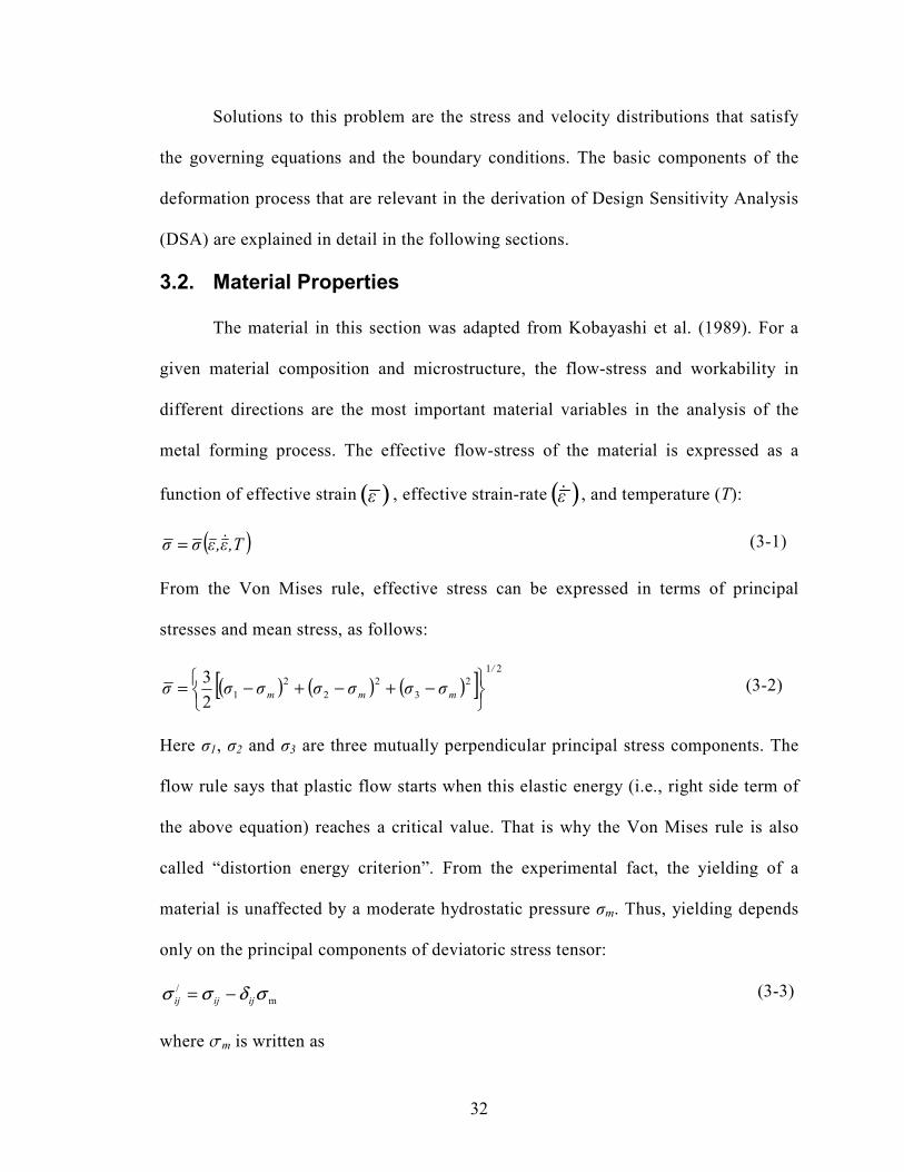
Solutions to this problem are the stress and velocity distributions that satisfy
the governing equations and the boundary conditions. The basic components of the
deformation process that are relevant in the derivation of Design Sensitivity Analysis
(DSA) are explained in detail in the following sections.
3.2. Material Properties
The material in this section was adapted from Kobayashi et al. (1989). For a
given material composition and microstructure, the flow-stress and workability in
different directions are the most important material variables in the analysis of the
metal forming process. The effective flow-stress of the material is expressed as a
function of effective strain ( )ε , effective strain-rate ( )ε& , and temperature (T):
( ),Tε,εσσ &= (3-1)
From the Von Mises rule, effective stress can be expressed in terms of principal
stresses and mean stress, as follows:
( ) ( ) ( )[ ]21
2
3
2
2
2
12
3/
mmm σσσσσσσ
−+−+−= (3-2)
Here σ1, σ2 and σ3 are three mutually perpendicular principal stress components. The
flow rule says that plastic flow starts when this elastic energy (i.e., right side term of
the above equation) reaches a critical value. That is why the Von Mises rule is also
called “distortion energy criterion”. From the experimental fact, the yielding of a
material is unaffected by a moderate hydrostatic pressure σm. Thus, yielding depends
only on the principal components of deviatoric stress tensor:
m
/ σδσσ ijijij −= (3-3)
where sm is written as

33
( )3213
1σσσσm ++= (3-4)
Then, the effective stress can be expressed as
( ) 21
2
3 //
ij
/
ijσσσ = (3-5)
3.3. Effective Strain and Effective Stress
The material in this section was adapted from Kobayashi et al. (1989). The
flow stress σ , is determined from a uni-axial test. Under multi-axial deformation
conditions, it is necessary to relate uni-axial material behavior to multi-axial material
behavior. Considering an element and the principal directions, the deformation energy,
dW, expended during time ∆t, over volume V, is
( )VdεσdεσdεσdW 332211 ++= (3-6)
Or divided by dt, the deformation power is
( )VεσεσεσP 332211&&& ++= (3-7)
Deformation energy in terms of the effective strain ε and effective strain-rate ε& are
written as: Vε dσdW = or Vε σP &= (3-8)
By substituting equation (3-8) in equation (3-7), we get
332211 εσεσεσεσ &&&& ++=⇒ (3-9)
From the volume constancy rule, 0321 =++ εεε &&& (3-10)
By using the Von Mises criterion, the effective strain-rate becomes
( ) ( ) 212
3
2
2
2
13
2
3
2 /
ijijεεεεεε &&&&&& =++= (3-11)
and the effective strain is obtained by integrating the effective strain over time.

34
3.4. Equilibrium Equations
The material in this section was adapted from Kobayashi et al. (1989). The
equilibrium equations with body forces fi, in suffix notation are written as
0=+ iij,j fσ (3-12)
In the rectangular coordinates, they can be expanded as follows:
0=+∂
∂+
∂
∂+
∂
∂x
xzxyxx fz
σ
y
σ
x
σ (3-13)
0=+∂
∂+
∂
∂+
∂
∂y
yzyyyxf
z
σ
y
σ
x
σ (3-14)
0=+∂
∂+
∂
∂+
∂
∂z
zzzyzx fz
σ
y
σ
x
σ (3-15)
3.5. Plastic Potential Equation
The material in this section was adapted from Kobayashi et al. (1989). In the
plastic deformation range, the stress and plastic strain-rate relationships are derived
using the concept of plastic potential. The ratios of the components of the plastic
strain-rate p
ijε& are defined by
fσ
ghε
ij
p
ij&&
∂
∂= (3-16)
where g and h are scalar functions of the invariants of deviatoric stresses and f is yield
function. The function ( )ijσg is called plastic potential. For a simple case, g=f is taken.
For a rigid-viscoplastic material, the constitutive equation becomes
/
ij
ij
ijp
ij σσ
ελ
σ
)f(σε
2
3&&& =∂
∂= where fhλ && = (3-17)

35
The material can also be assumed as linear viscous material for the initial guess or for
calculation of velocity fields (Oh et al (1982)). Then the constitutive equation can be
written as
ij
/
ij εµσ &2= (3-18)
where µ is viscosity. The solution of the rigid-viscoplastic material becomes identical
to that of the fictitious linear viscous material with the following viscosity:
( )ε
σεµµ
&&
3== (3-19)
3.6. Virtual Work-Rate Principle
The material in this section was adapted from Kobayashi et al. (1989). The
virtual work-rate principle states that for the stress field that is in equilibrium within
the body and with applied surface tractions, the work-rate inside the deforming body
equals the work-rate done by the surface tractions for all velocity fields that are
continuous and continuously differentiable (compatible). The compatibility
conditions in tensor notation are
( )j,ii,jij uuε +=2
1& (3-20)
ui,j is the differentiation of velocity components ui with respect to spatial directions xj.
The relation can be rewritten in an unbridged notation as follows:
∂
∂+
∂
∂=
i
j
j
iij
x
u
x
uε
2
1& (3-21)
Let ijσ be any stress field that is in equilibrium and uj be any virtual velocity field.
Then the principle is expressed by

36
∫∫ =S
jj
V
ijij dSuFdVεσ & (3-22)
3.7. Boundary Conditions
The material in this section was adapted from Kobayashi et al. (1989). In
metal forming analysis, the boundary conditions are divided into three types. They are
velocity boundary conditions, traction boundary conditions, and contact boundary
conditions.
3.7.1. Velocity Boundary Conditions
The velocity boundary conditions on Su are essential boundary conditions. In
finite element analysis, the velocity boundary conditions are enforced only at nodes
on Su, can be expressed as
ui = Ui on surface Su (3-23)
3.7.2. Traction Boundary Conditions
The stress along the boundary surface S is in equilibrium with an applied
traction fi (force per unit surface area). Equilibrium of the stress is written as
jiji nσf = (3-24)
where nj is the unit normal to the surface. Writing in an unbridged notation in the
two-dimensional case,
+
=
ll d
dxσ
d
dyσf xyxx
(3-25)
+
=
ll d
dxσ
d
dyσf yyxyy
(3-26)
where the components of the unit outward normal nj are given by (dy/dℓ, dx/dℓ), as
shown in Fig. 6.

37
Fig 6. Equilibrium of Surface Tractions
From the Fig. 6, the traction force fi acts normal to the surface S. This is
decomposed in x and y-directions as fx and fy. By applying equilibrium of forces
principle, Σfx = 0 and Σfy = 0, we can obtain the traction forces as in equations (3-25)
and (3-26).
3.7.3. Contact Boundary Conditions
The traction boundary condition on SF, is either zero-traction or ordinarily at
most a uniform hydrostatic pressure. However, the boundary conditions along the die-
workpiece interface are mixed. In general, neither velocity nor force can be prescribed
completely along this interface, because the direction of frictional stress is opposite to
the direction of relative velocity between the deforming workpiece and die, and this
relative velocity is not known priori.
In steady-state metal forming processes like extrusion, drawing the direction
of metal flow relative to die is known. In these problems, the frictional stress is given
according to the Coulomb law, i.e., fs=µp, or the friction law of constant factor m,
n
S
y
x dx
dy
0
dℓ
S
0
dℓ
x
y
fx dℓ
fy dℓ
fi dℓ
σy dx
τyx dx
σx dy
τxy dy

38
expressed by fs=mk (where 3Yk = ); here p is the die pressure and k is the shear
yield stress.
For nonsteady-state forming processes, for example, ring compression,
forming and roll forming, the direction of relative velocity between die-workpiece
interface is unknown. Moreover, the shapes of the dies change considerably from
process to process. Hence, frictional stress direction varies significantly. A unique
feature of the analysis is that there exists a point along die-workpiece interface where
the velocity of the deforming material relative to the die becomes zero. This point is
called “neutral point.” In order to deal with these situations, Oh et al. (1982)
approximated the friction stress with the arctangent function of relative velocities. At
the die-workpiece interface the traction boundary condition is expressed as
−≅−= −
0
1tan2
u
∆vmk
π∆v
∆vmkf s
s
ss
(3-27)
here fs is frictional stress, ∆vs is slipping or relative velocity, m is friction factor, k is
local flow stress in shear, and u0 is a small positive number compared to ∆vs. The
reason for using arctangent approximation is, it eliminates the sudden change of
direction of the frictional stress fs=mk, at the neutral point. The frictional stress
approaches ‘mk’ asymptotically as the relative sliding velocity us increases.
For any arbitrary die shape, the die-workpiece interface velocity boundary
conditions are applied in terms of normal velocities un as shown in Fig. 7. They can
be expressed as
un = vDn (3-28)
where vD is die velocity and n is the unit normal as shown in Fig. 7.

39
Fig 7. Schematic Diagram of Curved Die and Workpiece
3.8. Design Objectives
In metal forming, the material processing regions are governed by deformation
rates, temperature, and current state of plastic strains. The objective of any metal
forming process die designer is to obtain defect free product with minimum energy. In
practice, defects include dimensional distortion, internal or surface cracks, folds,
underfill, and excessive material wastage, local strains, and residual stresses.
Nonsteady metal forming processes such as forging is characterized by transient
contact boundary conditions along with geometric and material nonlinearities.
Therefore, one should include transient computations in die design. However as
mentioned in literature review boundary integral approach is new to metal forming
community. Therefore, the current research concentrated on only steady-state metal
forming process. Since the process is steady-state, a one time steady-state solution
can be considered for the analysis.
One of representative steady-state processes is extrusion. The main goal in
extrusion is to avoid bending, twisting, and dimensional inaccuracies in extruded part.
Local strain and exit velocity distributions heavily determine these quantities and are
one of the critical parameters that affect final extrude quality. Hence, the general
n s
Die Surface
Workpiece

40
objectives that can be considered as objective functions in the extrusion problem are
volume weighted strain variance (measure of strain variation) and exit velocity
variance. Strain variance/variation is computed on the component domain and the
average exit velocity is determined from the nodal velocities along the exit boundary
and is a boundary integral.
Therefore, a shape optimization problem for the extrusion problem can be
formulated for minimizing the strain variance (strain variation) or exit velocity
variance. To minimize objective function in optimization, the current initial guess die
shape should be moved in such as way that the new shape reduces the objective
function value while satisfying any specified constraints. The direction of the
movement is computed from sensitivity/gradient information of these objective and
constraint functions. Thus, sensitivity analysis is the heart of optimization algorithm,
on which current research focused. A general sensitivity analysis and optimization
procedure is presented in the following Chapter 4.
The main tools in SDSA are material derivative concepts for deforming
continuum. Prior to the actual derivation of the sensitivity, some of the material
derivative concepts are outlined to provide basic background about the procedure.

41
4. Design Sensitivity Analysis
In problems of optimal die shape design, geometric shape variables such as
locations of boundaries, and interfaces are considered as design variables. Such
problems cannot be easily reduced to a formulation that characterizes the effect of
shape variation explicitly in terms of a design function. Determination of the effect of
a shape change on a performance functional is the problem of “Shape Design
Sensitivity Analysis (SDSA),” which plays a central role in shape optimization
algorithms. A general die shape optimization algorithm and the role of sensitivity
analysis in the optimal design are presented in this Chapter (shown in Fig. 8).
An initial guess of the die shape is provided as a preliminary input to a shape
optimization algorithm. The only known data prior to design is the final desired
geometry and properties. These final desired properties such as exit velocity, die fill,
hardness, etc., are utilized in defining objective and constraint functions. These
objective and constraint functions are defined in terms of the process state variables
such as displacements, stresses, strain-rates, and strains, which can be obtained from
Finite Element Analysis (FEA) of the deformation process. The goal of design
process is to achieve an optimum shape that gives required performance. Sensitivities
or gradients provide the search direction for the optimization process. They provide
the effect of die shape change on the process performance criteria. In general, the
objective and constraint functions can be expressed as a combination of domain and
boundary integrals. Therefore, the formulated function integrals are then

42
differentiated to obtain the gradient expressions. However, due to the nonlinear nature
of the metal forming process, the differentiated expression is not straight forward to
compute. In order to achieve a computable formulation, the governing continuum
equations of deformation mechanics are utilized. Therefore, the sensitivity analysis is
termed as continuum sensitivity analysis. The basic procedure of continuum
sensitivity analysis and its components are outlined in the following section. Then the
computed sensitivities are supplied to an optimization routine, which are used to find
a new design point. Thus, the optimization is repeated until the convergence of the
results.
Fig 8. General Shape Optimization Procedure
Compute objective and constraint
functions
Input data
Initial trial shape
Final desired performance criteria
Perform finite element analysis
Obtain state variables
Call optimization routine
New shape design
Optimum shape
Y
N
Update shape
Continuum sensitivity analysis
• Utilize deformation mechanics • Formulate explicit sensitivity expression
Is design
satisfied?

43
4.1. Continuum Sensitivity Analysis
For optimal shape design, the sensitivity information can be obtained by finite
difference, semi-analytical, and analytical methods. Although easy to implement, the
finite difference method is computationally expensive and inaccurate. The accuracy of
the sensitivity information can be crucial for practical convergence in optimization.
Among all the sensitivity techniques, analytical techniques are proven to be superior
and hence, the current research focused on derivations of analytical sensitivity
formulas for forming operations. As discussed in section 2, analytical methods can be
discrete that utilize the finite element equations, and continuum, utilizes governing
equations of the process mechanics. Since, the finite element equations are not
available in commercial analysis packages, continuum approaches are gaining
importance over discrete methods. There are two classes of methods that can be
employed with continuum approach. They are Direct Differentiation Method (DDM),
which provides sensitivity information at every point of the continuum and Adjoint
Variable Method (AVM), which provides sensitivity information for one or more
performance functionals. DDM requires the solution of the system of equations once
for each design variable where as AVM only needs to solve the solution once for one
constraint. Usually, the number of design variables is more than the number of active
constraints in a shape design problem. Hence, the adjoint variable method is used in
the optimization problem.
Other important criterion in continuum sensitivity analysis for forming
problems is the type of framework for analysis, i.e., Lagrangian vs. Eulerian
framework.

44
4.1.1. Lagrangian Framework
In metal forming problems, a simple initial shape continuously changes upon
the application of compressive forces. In FEM analysis, the domain is subdivided into
a number of elements on which the solution is approximated with simple basic
functions. Forming processes are characterized as path dependent problems, i.e. the
history of the material has to be taken into account. For this reason, the updated
Lagrangian method is applied in the simulation of the forming processes [Kobayashi
et al. (1989)]. In this method the deformation path is approximated by increments in
time. After each increment the reference situation is updated with the velocity
solution. This updated situation is used as an initial condition for the next increment.
So, the finite element mesh is connected with the material through out the calculation.
The effective strains, instantaneous values, are obtained from the velocity solution at
each time step. These effective strains are added incrementally for each element to
determine the effective strains after a certain amount of deformation. A simple
schematic representation of Lagrangian description for material deformation is shown
in Fig. 9.
Fig 9. Lagrangian Description for Material Deformation
In Lagrangian approach the mesh moves with the material, and the field
variables that are obtained at the end of the simulation, are functions of initial shape.
Material and grid
moving direction
Compressed mesh
Grid Material
Ram

45
They are obtained as an integral over time domain. For example, effective strain is
expressed as the integration of effective strain over time domain ‘t’, is expressed as:
∫=t
dtεε0
& (4-1)
The final shape is function of initial shape x0 and integration of velocities over time
domain ‘t’, is written as
∫+=t
tf dtvxx0
0 (4-2)
Hence, the final objective and constraint functions become transient with
respect to time domain and also with respect to shape. Thus, the sensitivities that are
calculated using final field variables on the final shape have to be transformed to
initial configuration, which includes issues such as re-mesh, volume loss, change of
boundary conditions and updating the field variables. All these characteristics make
the problem complex.
4.1.2. Eulerian Framework
Except at the start and the end of the deformation, processes such as extrusion,
drawing, and rolling are kinematically steady-state. In steady-state problems, a mesh
fixed in space (Eulerian) is appropriate, since die configuration does not change with
time. Unlike in nonsteady-state process, the direction of velocity fields is constant
with time. The schematic Eulerian representation of the process is shown in Fig. 10.
Fig 10. Eulerian Description of Material Deformation
Material
moving
direction
Material Grid
Fixed grid
46
In Eulerian approach the mesh does not change with material. Hence, there is
no mesh distortion occurs. Thus, there is no need to apply transformation on the
sensitivities, because the initial and final shapes are the same. However, the material
non-linearity should be considered in the formulation.
Steady-state forming processes are being analyzed using Eulerian framework
in commercial analysis packages [ABAQUS]. Since the work is focused on steady-
state problems, Eulerian framework is used in the sensitivity formulations. Before
discussing the actual sensitivity derivation process, the following material derivative
concepts [from Choi et al. (1983) and Haug et al. (1986)] are presented to familiarize
the reader with notations and terms that come across in the derivation process. Please
see references for further details.
4.2. Material Derivative Concepts
A first step in SDSA is the development of the relationship between a
variation in shape and the resulting variations in functions that arise in the shape
design problems. Since the shape parameters of the domain Ω of a component are
treated as the design variables, it is convenient to think of Ω as a continuous medium.
The notion, shape as a continuous medium, is utilized in the material derivative
formulations.
4.2.1. Material Derivative Definition
Consider a domain Ω in two dimensions, and treat the domain as moving
continuum with time parameter t. The transformed domain at time t, is Ωt, as shown
schematically in Fig. 11. A small change in shape or domain is described by
transformation T, which is a function of previous spatial point and time, can be
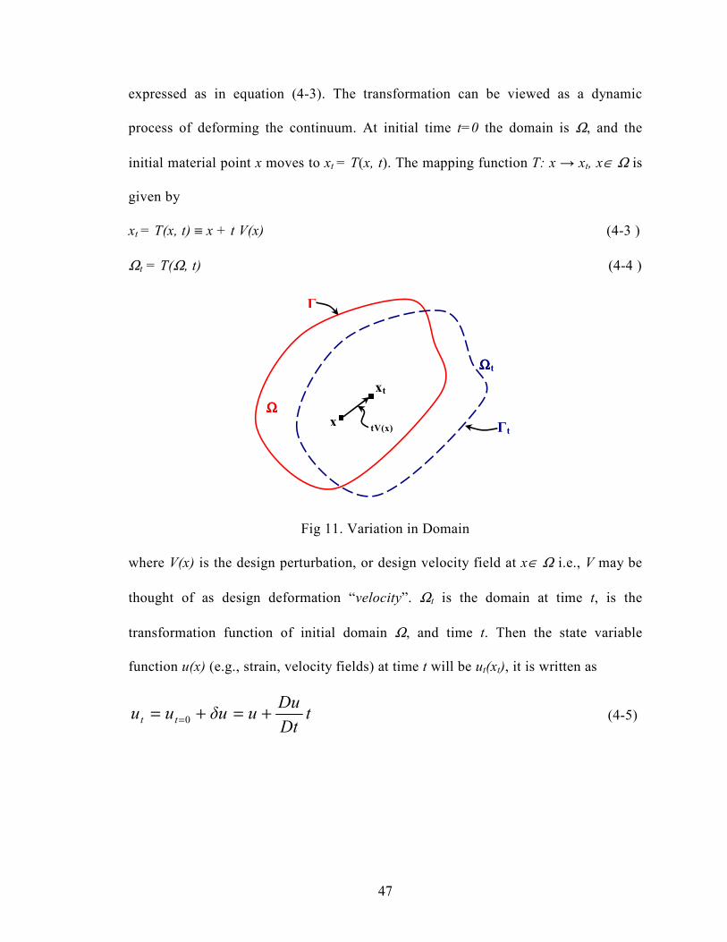
47
expressed as in equation (4-3). The transformation can be viewed as a dynamic
process of deforming the continuum. At initial time t=0 the domain is Ω, and the
initial material point x moves to xt = T(x, t). The mapping function T: x → xt, x∈ Ω is
given by
xt = T(x, t) ≡ x + t V(x) (4-3 )
Ωt = T(Ω, t) (4-4 )
Fig 11. Variation in Domain
where V(x) is the design perturbation, or design velocity field at x∈ Ω i.e., V may be
thought of as design deformation “velocity”. Ωt is the domain at time t, is the
transformation function of initial domain Ω, and time t. Then the state variable
function u(x) (e.g., strain, velocity fields) at time t will be ut(xt), it is written as
tDt
Duuδuuu tt +=+= =0 (4-5)
ΩΩΩΩ
ΩΩΩΩt
x
xt
Γ
Γt tV(x)

48
Here δu is the variation in state variable and it can be expressed as: tDt
Duδu = . The
displacement at time t (ut) is a function of x and t, and hence by using the chain rule
of differentiation, the velocity component of u can be written as
u.Vt
u
Dt
Du∇+
∂
∂= (4-6)
This velocity component is called material derivative of the state variable u. In tensor
notation, displacement material derivative can be written as
i,i
/ Vuuu +=& (4-7)
In general, objective or constraint functions are expressed as a boundary or
domain integral. Therefore, the material derivative procedure and including terms for
boundary and domain integrals are presented in the following sub-sections.
4.2.2. Material Derivative of a Functional on Boundary
Let any objective or constraint functional Φ (function of function) on a
boundary (Γ) is a function of the state variable u. Then the boundary integral can be
written as
∫=Γ
ψ(u) dΓΦ (4-8)
here )ψ(u denotes any arbitrary continuous function of u on boundary, and dΓ is
infinitesimal arc segment on the boundary. By using the chain rule of integration, the
material derivative of the functional Φ is written as
) ΓψddΓψ(ΦΓ
&&& += ∫ (4-9)

49
Here Γd & is the material derivative of an infinitesimal arc, it can be expressed as
dΓDVΓd s=& . DVs is the simplified notation of the boundary variable derivative terms
(velocity, tangential, and normal components of spatial coordinates). The complete
derivation is presented in the following section. The material derivative of an arc
segment can be divided into two components (Figures 12 and 13).
a) Normal component
b) Tangential component
4.2.2a. Normal Component
Normal component of the arc segment material derivative is obtained by
analyzing the normal velocity component Vn of the boundary. The length of the
infinitesimal arc changes because of the movement in the domain with time (Fig. 11).
The length of the arc segment at time t = 0 is dΓ. The new arc length at time t is dΓt.
It can be written as
tΓddΓdΓ t&+= (4-10)
The change in the length with time is tΓd & , shown schematically in Fig. 13.
Fig 12. Material Derivative of An Arc Segment, Normal Component
Hρ
1=
dθθθθ = HdΓ
t = 0
t = t
dΓ
dθθθθ
Vnt
tΓd &

50
The change in the boundary in normal direction is expressed with the help of
normal velocity component Vn as Vnt. The radius of curvature ρ is written as H
ρ1
= ,
where H is curvature boundary sector. From the Fig. 12, the change in length can be
written as
t)HdΓ(Vt)dθ(VtΓd nn ==& (4-11)
HdΓVΓd n=⇒ & (4-12)
Therefore, the normal component of the arc segment material derivative can be
written as
HdΓVΓd n=& (4-13)
4.2.2b .Tangential Component
There exist normal and tangential velocity components for the moving
boundary. Hence, the change in length of arc segment also occurs due to tangential
velocity component. The arc ab changes to a/b/ with time t (Fig. 13).
Fig 13. Material Derivative of An Arc Segment, Tangential Component
(Vs+Vs,sdΓ)t
Vst
t = 0
t = t
dΓ
a
b
a/
b/

51
The change in tangential velocity component from b to b/ is Vst, and hence the
corresponding change from a to a/ is (Vs+Vs,sdΓ)t. The change in arc length due to
tangential component Vs is equal to:
(Vs t)–(Vs t-Vs,s dΓ t) = Vs,st dΓ (4-14)
But we have the Actual change in length from Fig. 13 as tΓd & . Hence, from equations
(4-14), the change in arc length due to tangential component can be written as
t dΓVtΓd s,s= & (4-15)
Therefore, the total material derivative of arc segment is obtained by adding
equations (4-13) and (4-15), and is written as
( )dΓVHVΓd s,sn +=& (4-16)
4.2.2c. Vs,s Computation
In equation (4-16), the derivative of tangential velocity Vs,s is unknown. Hence,
a simplification is provided here. The tangential component of velocity vector Vs can
be written in a tensor notation as
Vs = Vk sk (4-17)
Then by differentiating the equation (4-17) with tangential component s, we can
write the Vs,s as
Vs,s = Vk,ssk+Vks,s (4-18)
In the above equation (4-18), Vk, Vk,s and sk can be computed explicitly. But the
first-order tangential derivative of the tangential component i.e., s,s needs further
simplification.
4.2.2d. Tangential Derivative of Normal n and Tangential s components

52
In this section the first-order derivatives of the normal and tangential
components (n and s) with respect to s is discussed. At point b in Fig. 14, the tangent
and normal components are s and n, respectively.
Fig 14. Tangential Derivatives
As the point moves on boundary from to a, the change in the components are
“sk,s dΓ” and “nk,s dΓ” for tangent and normal components, respectively. From the
above Fig. 12, the change in normal component can be expressed as
n,s dΓ= dθ sk = HdΓ sk (4-19)
⇒ n,s = H sk (4-20)
Similarly the change in tangent component can be expressed as,
s,s = –H nk (4-21)
Substituting equation (4-21) in the equation (4-18) for Vs,s,
⇒ Vs,s = Vk,ssk+Vks,s = Vk,ssk – HnkVk = Vk,ssk – HVn (4-22)
The arc segment material derivative is obtained by substituting equation (4-22) in
equation (4-16) as
( ) dΓsVdΓHVsVHVΓd kk,snkk,sn =−+=⇒ & (4-23)
Let kk,ss sVDV = , then the equation (4-23) becomes
dΓ
dθθθθ = H dΓ
n
n+n,s dΓ
s
s+s,s dΓ
a
b

53
dΓDVΓd s=& (4-24)
Note here that DVs is just a notation for simplicity. It does not carry any physical
meaning. Similarly, for normal component, DVn can be introduced as follows
kk,sn nVDV = (4-25)
Some of the other material derivatives that can be used in the derivation are s&
and n& . The physical interpretations of these derivatives are explained in the following
sections.
4.2.3. Material Derivative of s
When the boundary changes with time t, the tangential component s also
changes. The change is a cumulative effect of normal and tangential direction changes.
4.2.3a. Normal Component
The change in s in normal direction is schematically shown in Fig. 15. The arc
ab is changed to a/b/ with time. From time t=0, the tangential component s, is changed
to τss &+ .
Fig 15. Material Derivative of s, Normal Component
The change in position from b to b/ is Vnt, and the corresponding change in
position from a to a/ is (Vn + Vn,s dΓ)t. Here Vn,s is the change in Vn in tangential
(Vn+ Vn,sdΓ)t
a
ts&
tss &+ s
dΓ s
tss &+
dθθθθ Vnt
t = t
t = 0
a/
b
b/

54
direction. From Fig. 15, the change in tangential component is ts& , and it points
towards the same direction as n. For any unit tangential vector s, the change in
component can be expressed as
n dτs θ=& (4-26)
here dθ can written as
tVdθ n,s = (4-27)
By substituting equation (4-27) in equation (4-26), we get the material derivative of
tangential component in normal direction as
nVsn tV ts n,sn,s =⇒=⇒ && (4-28)
4.2.3b. Tangential Component
Consider the tangential change in s with time, as shown in Fig. 16. The change
in s from point a to a/ with time is ts& . The length of a-a
/ is written as Vs t.
Fig 16. Material Derivative of s, Tangential Component
From figure 17, the angle of suspension, dθ, is written as
tH Vρ
tVdθ s
s == (4-29)
ts& tss &+
s
dθθθθ
t = 0, t = t
H1ρ =
s
τss &+
Vst
dθθθθ
a
a/

55
The change in s, acts in opposite direction to normal vector n. Hence, the change can
be written as
ndθ ts −=⇒ & (4-30)
By substituting equation (4-29) in equation (4-30), the material derivative of s, in
normal direction is obtained as follows
n tH V ts s−=⇒ & (4-31)
Therefore, the total material derivative of the tangent component s is written
by adding equation (4-28) and equation (4-31)
H) nV(Vs sn,s −=& (4-32)
These definitions of material derivative terms will be used in sensitivity derivation.
4.3. Sensitivity Derivation
A general shape design sensitivity formulation for the steady-state forming
process is derived in this section (Fig. 17) by using DSA concepts that were explained
in previous sections.
The sensitivity derivation starts by deriving the identity integral from
deformation process governing equations. The basic continuum plasticity equations,
equilibrium, compressibility, material constitutive laws, and boundary conditions are
the input data for the derivation. Corresponding to the actual solution variables of the
metal forming analysis, velocity field u and pressure p, and a couple of arbitrary
variables (u* and p
*) are introduced. These arbitrary variables are called as adjoint
variables. By applying integration on the continuum equations over the domain, an
identity integral is obtained. The integral identity is then differentiated using material
derivative concepts.

56
Fig 17. Continuum Sensitivity Analysis Approach
The objective and constraints are generally functions of state variables and
can be expressed as domain or boundary integrals. Sensitivity analysis focus is to
obtain the change in objective and constraints with respect to change in design
variables. Hence, objective and constraint integrals are differentiated with respect to
design variables by using material derivatives concepts. However, the material
derivative of objective and constraint functional include the unknown terms. These
unknown terms are eliminated by defining an adjoint problem, which makes use of
the material derivative of identity integral. In adjoint problem, the shape of the metal
forming product remains same as in the actual simulation and the boundary conditions
change based on the required process performance. Then an explicit sensitivity
formula is obtained as a function of actual state variables, adjoint variables, and shape
variables. The basic components of the approach and the derivation steps are clearly
presented in the following sections.
Obtain objective/constraint
functions
Define adjoint continuum
conditions and finite
element analysis
Obtain sensitivity formula
Continuum plasticity equations
Identity integral
formulation
Finite element analysis
Material
derivative
formulations

57
4.3.1. Identity Integral Formulation
As explained before, the primary component of sensitivity derivation is to
obtain the identity integral by using equilibrium, and compressibility equations of
deformation process.
Consider velocities ‘ui’ that satisfy the equilibrium equations
0=+ iij,j fσ (4-33)
where fi is distributed force on the domain, σij and σij,j are the stress field and their
derivatives in spatial directions, respectively.
From equation (3-10), the incompressibility condition is expressed as
0== iii,i εu & (4-34)
Recalling from section 3, the stress tensor is given by
pδσσδσσ ij
/
ijmij
/
ijij −=−= (4-35)
where /
ijσ is deviatoric stress and
≠
==
ji
ji δij
K
K
0
1 and p is mean stress. The
constitutive equation of the deformation process is given as
ij
/
ij εσ
εσ &
&
2
3= (4-36)
here, σ is effective flow stress, a function of strain-rate, strain and temperature for
visco-plastic materials; ( ),Tε,εσσ &= is defined by
2123 //
ij
/
ij .σσσ = (4-37)
In metal forming, for work hardening materials the effective flow stress can be
written as:
( ) nεKεσσ && == (4-38)

58
here n is strain sensitivity and K is material constant.
From equation (3-11), the effective strain-rate is given as
21
3
2εεε ijij
&&& = (4-39)
By substituting equation (4-38) in equation (4-36), the expression for deviatoric
stress is obtained as [Joun et al. (1998)]:
ijijn
/
ij εεεK
εσ &&
&
& 2
2
3α== (4-40)
where
)ε(4K
ε3 n1
&&
αα ==−
(4-41)
Introduce an arbitrarily weighted adjoint variable u*, multiply the equilibrium
equation (4-33) and integrate over domain.
0 =+∫Ω
*
iiij,j dΩu)f(σ (4-42)
By simplifying equation (4-42), we will get the following equation:
∫∫∫ =+=+Ω
*
ii
Ω
*
iij,j
Ω
*
iiij,j dΩufdΩuσdΩu)f(σ 0 (4-43)
Simplify the first term on right hand side of equation (4-43) by integration by parts as
∫∫∫ −=Ω
*
i,jijj
*
i
Γ
ij
Ω
*
iij,j dΩuσ dΓnuσ dΩuσ (4-44)
Let traction forces jiji nστ = , then the equation (4-44) becomes
∫∫∫ −=Ω
*
i,jij
*
i
Γ
i
Ω
*
iij,j dΩuσ dΓuτ dΩuσ (4-45)
Using equation (4-35), substitute the stress tensor expression in equation (4-45), then,

59
∫∫∫
∫∫∫
+−=
−−=
Ω
*
i,jij
Ω
*
i,j
/
ij
*
i
Γ
i
Ω
*
i,jij
/
ij
*
i
Γ
i
Ω
*
iij,j
dΩp uδ dΩuσ dΓuτ
dΩp) uδ(σ dΓuτ dΩuσ
(4-46)
Then substitute equation (4-46) in equation (4-43)
∫∫∫∫∫ =++−=+Ω
*
ii
Ω
*
i,jij
Ω
*
i,j
/
ij
*
i
Γ
i
Ω
*
iiij,j dΩuf dΩp uδ dΩuσ dΓuτ dΩ) uf(σ 0 (4-47)
Simplify equation (4-47) by moving the third term of right hand side to left side of the
equation gives:
∫∫∫∫∫ +−=−+Ω
*
ii
Ω
*
i,j
/
ij
*
i
Γ
i
Ω
*
i,jij
Ω
*
iiij,j dΩuf dΩuσ dΓuτ dΩp uδdΩ) uf(σ (4-48)
here second term on left side can be written as
*
ii
*
i,i
*
i,jij εuuδ &== (4-49)
By using incompressibility property of deformation process, from equation (4-34) and
the equilibrium conditions from equation (4-33), the equation (4-48) can be rewritten
as
0=+−⇒ ∫∫∫Ω
*
ii
Ω
*
i,j
/
ij
*
i
Γ
i dΩuf dΩuσ dΓuτ (4-50)
The assumed variable u* satisfies an adjoint governing equation. Then the adjoint
equilibrium equation is written as
0=+ *
i
*
ij,j fσ (4-51)
Incompressibility condition for adjoint problem is expressed as
0== *
ii
*
i,i εu & (4-52)
And the material constitutive law for an adjoint system is
*
ij
*/
ij εσ & 2α= (4-53)

60
By following similar procedure from equation (4-42) to (4-50), we get another
integral for primal variable u, as follows
0=+− ∫∫∫Ω
i
*
i
Ω
i,j
*/
iji
Γ
*
i dΩuf dΩuσ dΓuτ (4-54)
Obtain an identity integral by subtracting the equation (4-53) from equation (4-50)
0)dΩufu(f)dΩuσu(σ)dΓuτu(τΩ
*
iii
*
i
Ω
*
ji,
/
ijji,
*/
ij
*
iii
Γ
*
i =−+−−− ∫∫∫ (4-55)
By substituting material constitutive laws, equations (4-40) and (4-53), in
equation (4-55), the identity integral reduces to
0dΩ )ufu(fdΓ )uτu(τΩ
*
iii
*
i
*
iii
Γ
*
i =−+− ∫∫ (4-56)
The derived identity integral is further utilized to take the material derivative
and to define the conditions for adjoint analysis.
4.3.2. Material Derivative on Identity Integral
Once the identity integral is obtained, then the identity variation is computed
by applying the material derivative techniques. Consider the first term from equation
(4-56); which is an integral on boundary only. By taking the material derivative on
the boundary functional (section 4.3.2), the integral can be simplified as
( ) ( ) dΓ DVuτuτ dΓuτuτuτuτ s
Γ
*
iii
*
i
Γ
*
ii
*
iii
*
ii
*
i ∫∫ −+−−+ &&&& (4-57)
Now by taking the material derivative of the second term of equation (4-56), which is
domain integral, we will get
( ) ( )∫∫ −+−−+Ω
k,k
*
iii
*
i
Ω
*
ii
*
iii
*
ii
*
i dΩVufufdΩufufufuf &&&&
By rearranging the terms in above equation,

61
( ) ( )∫∫∫∫ −+−−+Ω
k,k
*
iii
*
i
Ω
*
ii
Ω
*
iii
*
i
Ω
i
*
i dΩ Vufuf dΩuf dΩufuf dΩuf &&&& (4-58)
The total material derivative on identity integral will be obtained by adding
two material components, i.e., equations (4-57) and (4-58). By rearranging the terms,
the resultant equation becomes
( ) ( ) ( )
( ) ( ) dΓ DVuτuτ dΓuτuτ
dΩufuf dΩ Vufuf dΩuf dΩuf dΓuτuτ
s
Γ
*
iii
*
i
Γ
*
iii
*
i
Ω
*
iii
*
i
Ω
k,k
*
iii
*
i
Ω
*
ii
Ω
i
*
i
Γ
*
iii
*
i
∫∫
∫∫∫∫∫
−−−−
−−−−=+−
&&
&&&&&&
(4-59)
By using material derivative definition, the material derivative of adjoint velocity
field can be written as
j
*
i,j
*/
i
*
i Vuuu +=& (4-60)
The material derive of traction forces are obtained as follows
( ) jnijjkij,k
/
ijjijjij i s DVσ nVσσnσnστ −+=+= &&&
nijkij,k
/
ii DVq n Vσττ −+=⇒ & (4-61)
where qi is tangential component of stresses, written as: jiji sσq =
Similarly for adjoint tractions, the material derivative can be expressed as
n
*
ijk
*
ij,k
*/
i
*
i DVq n Vσττ −+=⇒ & (4-62)
The material derivative for the body forces is expressed as
j Vff i,ji =& (4-63)
j
*
i,j
*
i Vff =& (4-64)
Now equation (4-59) is simplified by substituting the equations from (4-60) to (4-64)
First term in equation (4-59) on the right hand side is:

62
( ) ( )∫∫ =Ω
*
iki,k
Ω
*
ii dΩuVf dΩuf& (4-65)
Second term in equation (4-59) on the right hand side is:
( ) ( ) ( )∫∫∫ −−++−−=−−Ω
k
*
i,ki
*
ii,ki,k
*
ii
*
i,k
Γ
n
*
iii
*
i
Ω
k,k
*
iii
*
i dΩVufufufuf dΓVufuf dΩVufuf
(4-66)
Third term in equation (4-59) on the right hand side is:
( ) ( )∫∫ ++−=−−Ω
k
*
i,ki
*/
iiik
*
i,k
Ω
*
iii
*
i dΩVufufuVf dΩufuf && (4-67)
Fourth term in equation (4-59) on the right hand side is:
( ) ( ) dΓVuτuτ u DVqunVσuτ dΓuτuτΓ
k
*
i,ki
*/
iiin
*
iijk
*
ij,ki
*/
i
Γ
*
iii
*
i ∫∫ +++−−=−− && (4-68)
Now substitute equations from (4-65) to (4-68) in (4-59). Note here that the identity
integral (4-56) holds good for ui*/ (i.e., the derivation of adjoint velocity with respect
to time). Then the equation (4-59) becomes:
( ) ( )
) dΓVuτu DVqunVσ(
dΓ DVuτuτ dΩVuf dΓVufuf dΩuf) dΓuτuτ(
k
*
i,kii
Γ
n
*
iijk
*
ij,k
s
Γ
*
iii
*
i
Ω
ki,k
*
i
Γ
n
*
iii
*
i
Ω
i
*
i
*
iii
*
i
Γ
++−+
−−+−−=+−
∫
∫∫∫∫∫
&&&
(4-69)
Here, DVn and DVs are substituted from equations (4-24) and (4-25), then
( )kjkjk,s
*
ijkk,sj
*
ijkk,sj
*
ijs
*
in
*
i snnsVσsVnσnVsσ DVτ DVq −=−=−
( )kjkjjk snnse −=Q
jksk,
*
ijs
*
in
*
i eVσDVτDVq =−⇒ (4-70)
Substitute equation (4-70) in equation (4-69); then the equation (4-69) reduces to

63
( ) ( )
( )
( )∫
∫
∫∫∫∫
++
+−+
+−−=+−⇒
Γ
k
*
i,kis
*
ii
Γ
ijkk,s
*
ijijk
*
ij,k
Ω
ki,k
*
i
Γ
n
*
iii
*
i
Ω
i
*
i
Γ
*
iii
*
i
dΓVuτDVuτ
dΓueVσunVσ
dΩVuf dΓVufuf dΩuf dΓuτuτ
&&&
(4-71)
By simplifying equation (4-71) with the application of integration by parts formula
for the third term on right hand side of the equation, we get
( ) ( ) dΓ ueVσueV-σdΓueVσΓ
i,sjkk
*
ijijkk
*
ij,s
Γ
ijkk,s
*
ij ∫∫ −= (4-72)
By substituting equation (4-72) in equation (4-71), the equation becomes
( ) ( )
( )
( )∫
∫
∫∫∫∫
++
−−−+
+−−=+−⇒
Γ
k
*
i,kis
*
ii
Γ
ii,sjkk
*
ijijkk
*
ij,sijk
*
ij,k
Ω
ki,k
*
i
Γ
n
*
iii
*
i
Ω
i
*
i
Γ
*
iii
*
i
dΓVuτDVuτ
dΓueVσueVσunVσ
dΩVuf dΓ Vufuf dΩuf dΓuτuτ &&&
(4-73)
Again, simplify the third term in the equation (4-73), by substituting the following
relations:
)eσn(σVuueVσunVσ jk
*
ij,sj
*
ij,kkiijkk
*
ij,sijk
*
ij,k +−=−−
where k
*
ij,sk
*
ij,n
*
ij,k sσnσσ += and )snn(se kjkjjk −=
)snσnsσnsσnn(σVu)eσn(σVu kj
*
ij,skj
*
ij,sjk
*
ij,sjk
*
ij,nkijk
*
ij,sj
*
ij,kki −++−=−⇒
*
ij,jkkij
*
ij,sj
*
ij,nkki σnVu)sσn(σnVu −=+−⇒ (4-74)
By substituting the equilibrium equation (4-33) in (4-74), equation (4-74) becomes
iuVf)sσn(σnVu n
*
ij
*
ij,sj
*
ij,nkki =+−⇒ (4-75)
By substituting the above relations from (4-74) and (4-75), the material derivative of
the identity integral is obtained as follows:

64
( )
∫
∫∫∫
+++−+
=+−
Γ
n
*
iik
*
i,kis
*
iii,sjkk
*
ij
Ω
ki,k
*
i
Ω
i
*
i
Γ
*
iii
*
i
) dΓVufVuτDVuτueVσ(
dΩVuf dΩuf dΓuτuτ &&&
(4-76)
The derived material derivative is used in eliminating the unknown terms of
the objective function derivation.
4.3.3. Material Derivative of Objective/Constraint Functional
The next step in the approach is to compute material derivatives of the
objective or constraint functional. Consider a general objective/constraint functional
which consists of both the domain and boundary integral, is written as
( ) ( )∫∫ +=Γ
ii
Ω
dΓ,τuζ dΩεΦΨ & (4-77)
where ε& is effective strain-rate, ui is velocity field, and τi are traction forces. An
example of a domain integral can be effective strain variance, expressed as
( ) dΩεεΩ
ΦΩ
avg∫ −=21
(4-78)
where avgε is average strain. The effective strain is a function of strain-rate.
Some of the boundary integral objective functions are ram force in the
horizontal direction or vertical force applied to the die in extrusion. In the case of
contact boundary, the boundary integral becomes the function of tangential velocity
field and shear stress, as shown:
( ) dΓ ;mk,uτζζ
cΓ
ss ∫=
In this derivation, occurrence of tangential components, i.e., us, is neglected for
simplicity. The material derivative of the objective function (equation 4-77) becomes

65
∫∫∫∫ +++=Γ
s
ΓΩ
k,k
Ω
dΓζDV dΓζ dΩΦV dΩΦΨ &&& (4-79)
where ijε EΦΦ
ij
&&&
= , hereijE& denotes the material derivative of strain-rate.
(Note: E is used in place of effective strain-rate ε& , to avoid confusion with the
material derivative notation).
Simplify the second term in equation (4-79) as
∫∫∫∫ −=−⇒Ω
k,kijε,
Γ
n
Ω
k,k
Γ
n dΩVΦ dΓΦV dΩVΦ dΓΦVijε&
& (4-80)
Expand the third term of equation (4-79) as:
( )∫ +⇒Γ
iτiu dΓτζuζii&& (4-81)
By substituting equations (4-80) and (4-81) in equation (4-79) and simplifying:
( ) ∫∫∫∫∫ +++−+=Γ
s
Γ
iτiu
Ω
k,kijε,
Γ
n
Ω
ijε, dΓζ DV dΓτζuζ dΩVΦ dΓΦV dΩEΦΨiiijij&&&&&
&&ε (4-82)
Here the material derivative of strain-rate is written as
kij,k
/
ijij VεεE &&& += (4-83)
Substitute equation (4-83) in equation (4-82)
( ) ∫∫∫∫∫ +++−++=⇒Γ
s
Γ
iτiu
Ω
k,kijε,
Γ
n
Ω
kij,k
/
ijε, dΓζDV dΓτζuζ dΩVεΦ dΓΦV) dΩVεε(ΦΨiiijij&&&&&&
&&
Simplify,
( ) ∫∫∫∫ ++++=⇒Γ
s
Γ
iτiu
Γ
n
Ω
/
ijε, dΓζ DV dΓτζuζ dΓΦV dΩεΦΨiiij&&&&
& (4-84)
Effective strain is obtained by the integration of strain-rate quantities. Hence, strain-
rate partial derivatives can be utilized further in the derivation. Strain-rate
differentiation with respect to time can be written in terms of velocities from their
compatibility relations:

66
( )j,ii,jij uuε +=2
1&
( ) ( )/
ij
/
j,i
/
i,j
/
ij Uεuuε && =+=2
1 (4-85)
U denotes the vector notation of strains, which are the function derivatives of
displacements. We have the material derivative formula of displacement, from
equation (4-7) as
VUUU / ∇−= & (4-86)
Substitute equation (4-86) in equation (4-85), the partial derivative of strain becomes
( ) ( )U VεUεε ijij
/
ij ∇−= &&&& (4-87)
By substituting equation (4-87) in (4-84), the material derivative of objective function
is obtained as
( ) ( )
( ) ∫∫
∫∫∫
+++
+∇−=
Γ
s
Γ
iτiu
Γ
n
Ω
ijε,
Ω
ijε,
dΓζ DV dΓτζuζ
dΓΦV dΩVUεΦ dΩUεΦΨ
ii
ijij
&&
&&&&&&
(4-88)
Then the first term on the right hand side of equation (4-88) can be written as
( ) ( )∫∫∫ −=Ω
i,j
ε,
Γ
jiε,
Ω
ijε, dΩuΦ dΓnu Φ dΩUε Φijijij
&&&&&&&
(4-89)
Substitute equation (4-89) in equation (4-88). Then the material derivative of the
objective/constraint functional in terms of domain and boundary integrals becomes
( ) ( )
( ) ∫∫
∫∫∫∫
+++
+∇−+=
Γ
s
Γ
iτiu
Γ
n
Ω
ijε,
Ω
i,j
ε,
Γ
ijε,
dΓζDV dΓτζuζ
dΓΦV dΩVUεΦ dΩuΦ dΓunΦΨ
ii
ijijij
&&
&&&&&&&
(4-90)
In the above equation (4-90), the boundary integrals (third and fifth terms on right
hand side) are explicit in terms of velocity vectors, objective and constraint function

67
values. Hence, they can be computed from the FEM analysis output results. But the
material derivative terms i.e., iu&and
iτ&are unknown in nature. These have to be
replaced with known expressions. These relations are obtained by comparing equation
(4-90) with the material derivative of identity integral equation (4-76). This
elimination is done by defining an adjoint problem for the analysis.
4.3.4. Adjoint Problem Definition
Recalling equations (4-76) and (4-90), we rewrite them here.
Material derivative of integral identity:
( )
∫
∫∫∫
+++−+
=+−
Γ
n
*
iik
*
i,kis
*
iii,sjkk
*
ij
Ω
ki,k
*
i
Ω
i
*
i
Γ
*
iii
*
i
) dΓVufVuτDVuτueVσ(
dΩVuf dΩuf dΓuτuτ &&&
(4-76)
Material derivative of objective or constraint integral:
( ) ( )
( ) ∫∫
∫∫∫∫
+++
+∇−+=
Γ
s
Γ
iτiu
Γ
n
Ω
ijε,
Ω
i,j
ε,
Γ
ijε,
dΓζDV dΓτζuζ
dΓΦV dΩVUεΦ dΩuΦ dΓunΦΨ
ii
ijijij
&&
&&&&&&&
(4-90)
By rearranging terms in equation (4-90)
( ) ( )
( ) ∫∫∫
∫∫∫
++∇−
+++=
Γ
s
Γ
n
Ω
ijε,
Ω
i,j
,ε
Γ
iτ
Γ
iuj,ε
dΓζ DV dΓΦV dΩVUεΦ
dΩuΦ dΓτζ dΓu ζnΦΨ
ij
ijiiij
&
&&&&
&
(4-91)
By comparing the above two equations (i.e., 4-76 and 4-91), the right hand side terms
in equation (4-76) can be replaced in the place of unknown terms of equation (4-91).
This is true only when the coefficients of iu& and iτ& in equation (4-91) are equal to the
coefficients of corresponding terms in equation (4-76). This condition leads to
defining new set of boundary conditions as follows

68
iij ujε,
*
i ζnΦτ +=&
on boundary (A1)
iτ
*
i ζu −= on boundary (A2)
( ),j
ε,
*
i ijΦf
&= on domain (A3)
These conditions are called as adjoint boundary conditions. Thus, the adjoint analysis
is performed using these boundary conditions, where as the basic shape of the die
remains the same as in actual or primal analysis.
4.3.5. Sensitivity Formulation
Once the adjoint problem is defined, the equation (4-76) can be substituted
directly in equation (4-91). Then the objective or constraint sensitivity formula
becomes
( )
( ) ∫∫∫
∫∫
++∇−
+++−+=
Γ
s
Γ
n
Ω
ijε,
Γ
n
*
iik
*
i,kis
*
iii,sjkk
*
ij
Ω
ki,k
*
i
dΓζ DV dΓΦ V dΩVUεΦ
dΓVufVuτDVuτueVσ dΩVufΨ
ij &
&
&
(4-92)
By simplifying the third term on the right-hand side in equation (4-92) we get
( ) ( ) ( )∫∫∫ +∇−=∇−Ω
ki,k,j
ε,j
Γ
ε,
Ω
ijε, dΩVuΦ dΓ nU VΦ dΩU VεΦijijij &&&
& (4-93)
where ki,kVuU V =∇ , then the equation (4-93) becomes
( ) ( ) ( )∫∫∫ +−=∇−⇒Ω
ki,k,j
ε,j
Γ
ki,kε,
Ω
ijε, dΩVuΦ dΓn VuΦ dΩU VεΦijijij &&&
& (4-94)
Substitute equation (4-94) in equation (4-92)
( ) ( )
( ) ( ) ∫∫∫∫
∫∫
+++−
+++−+=⇒
Γ
s
Γ
n
Ω
ki,k,j
ε,
Γ
jki,kε,
Γ
n
*
iik
*
i,kis
*
iii,sjkk
*
ij
Ω
ki,k
*
i
dΓζ DV dΓΦV dΩVuΦ dΓnVuΦ
dΓVufVuτDVuτueVσ dΩVufΨ
ijij &&
&
(4-95)
By simplifying, the equation (4-95) becomes

69
( )
( ) ∫∫∫
∫
++−
+++−=⇒
Γ
s
Γ
n
Γ
jki,kε,
Γ
n
*
iik
*
i,kis
*
iii,sjkk
*
ij
dΓζ DV dΓΦV dΓnVuΦ
dΓVufVuτDVuτueVσΨ
ij&
&
(4-96)
Therefore, the derived sensitivity formula is
( )
( ) dΓζ DVΦVV u nΦ
dΓVufVuτDVuτueVσΨ
Γ
snki,kjε,
Γ
n
*
iik
*
i,kis
*
iii,sjkk
*
ij
ij∫
∫
++−+
+++−=∴
&
&
(4-97)
It can be observed that the above sensitivity formula consists of boundary
integration of primal and adjoint field variables (e.g., u and u*). It is an only explicit
formulation in terms of any FEM analysis results. The implementation of the DSA
result by using commercial software is given in the following section.
4.4. Implementation
Based on the derived sensitivity formula, gradients of the response with
respect to each design parameter can be evaluated. In practice, shape is generally
expressed by a number of geometric functions and their associated parameters. Then,
the design variables are those finite parameters that control the shape. If we denote
the design parameter set as b=b1, b2, …, bn, the boundary shape, i.e., the coordinates
of the boundary, is a function of these parameters as follows:
x = x(b), Γx ⊂ (4-98)
The shape variation/velocity vector V appearing in the sensitivity formula is related
by the design parameter as
i
n
i
n
i
ii
i
i b Vb b
xδx δδ∑ ∑
= =
=∂
∂=
1 1
(4-99)

70
which states that the shape variation vector is the change of the point x on the
boundary due to the variation of each design parameter. Therefore, n sets of the shape
variation vectors are necessary. After substituting equation (4-99) into the general
expression (i.e., equation 4-97), the sensitivity formula eventually becomes
i
n
i
n
i
ii
i
i
Γ
b GRADb dΓb
xu,w, ΨΨ δδ∑ ∑∫
= =
=
∂
∂′=′
1 1
(4-100)
here GRADi, is the gradient value for the design parameter bi, which is used in the
optimization routine.
Fig 18. Overall Procedure for Sensitivity Calculation
The overall procedure for the sensitivity calculation is given in Fig. 18. Once
the boundary shape variables bi, are defined, metal forming analysis can be performed
Define die shape parameters
Compute shape variation vector
Perform Adjoint FEM Analysis
Obtain adjoint state variables (u*)
(ABAQUS)
Compute adjoint boundary conditions
(MATLAB)
Perform Primal FEM Analysis
• Primal boundary conditions
• Obtain primal state variables (u)
(ABAQUS)
Compute Sensitivity
(MATLAB)
Prepare adjoint state variables database
(MATLAB)
Continuum plasticity
equations
Define objective and
constraint functions

71
under the actual boundary conditions. All the required field variables such as stresses,
strains, displacements, etc., are obtained from the primal analysis and stored in
MATLAB. The adjoint boundary conditions are computed using the derived
expressions. Then one more analysis is performed using these adjoint boundary
conditions, called adjoint analysis. The field variables from the adjoint analysis are
fed to MATLAB. Finally, gradients are computed using primal analysis field
variables u, adjoint analysis field variables u*, and shape variation velocity vector Vi,
in MATALB. The derived sensitivity formulations are implemented through extrusion
case study. The domain integral and boundary integral functional gradients are
computed. Further the accuracy of the sensitivity formulation is checked with finite
difference sensitivities.
4.5. Case Study - Extrusion
Extrusion is the process by which long straight metal parts can be produced.
The cross-sections that can be produced vary from solid round, rectangular, to L
shapes, T shapes. A sectional reduction of 75%, which leads to the development of
strain of order more than unity, is considered for the extrusion process. The material
nonlinearity is introduced through stress-strain curve. A finite element analysis is
performed with ABAQUS. Quadrilateral mesh is generated using automatic mesh
generator. In a steady-state process, an invariant pattern of deformation will be
developed relative to the die. Figure 19 shows such a steady-state process residual
pattern of deformation in the extruded sheet. It exhibits a translational invariance
along its length except for transient regions adjacent to the free end of the sheet and in
the neighborhood of the die. This is so since the material which has left the die is

72
subjected to no surface tractions, and each congruent cross-section has been subjected
to the same history of deformation followed by unloading to zero resultant load and
zero traction on the lateral surfaces.
4.5.1. Process and Boundary Conditions
An axisymmetric extrusion process boundary conditions and the mesh system
are shown in Fig. 19. An isothermal steady-state metal forming analysis is performed
using ABAQUS. The continuum conditions and the mesh system used for the analysis
of extrusion are shown in Fig. 19.
Fig 19. Finite Element Model Extrusion - Boundary Conditions
r
z
Entrance - uz = 5, τr = 0
Sym
metr
y l
ine u
r = 0, τz = 0
τr = 0
n
ℓ (τl = mk)
(un = 0)

73
The model geometry consists of a rigid die and a blank. The blank geometry is
defined such that it closely approximates the shape corresponding to the steady-state
solution: this geometry can be thought of as an “initial guess” to the solution. The
blank is discretized with a simple graded pattern that is most refined near the die fillet.
The blank is constrained at the axis of symmetry in the r-direction. Radial expansion
of the blank is prevented by giving contact boundary conditions between workpiece
and the die.
An adaptive mesh domain is defined that incorporates the entire blank.
Because the Eulerian domain undergoes very little overall deformation and the
material flow speed is much less than the material wave speed. The outflow boundary
is assumed to be traction-free and is located far enough downstream to ensure that a
steady-state solution can be obtained. This boundary is defined using the *SURFACE,
REGION TYPE=EULERIAN option. A multi-point constraint is defined on the
outflow boundary to keep the velocity normal to the boundary uniform. The inflow
boundary is defined by using the *BOUNDARY, REGION TYPE=EULERIAN option
to prescribe a velocity of 50 mm/sec in the vertical direction. Adaptive mesh
constraints are defined on both the inflow and outflow boundaries to fix the mesh in
the vertical direction using the *ADAPTIVE MESH CONSTRAINT option. This
effectively creates a stationary control volume with respect to the inflow and outflow
boundaries through which material can pass.
Symmetry of the die and workpiece about the center line permits the solution
to be carried out on the half the billet only, on the one side of the center-line. The
shear and the normal velocity on this symmetry line would be zero. Usually, extrusion

74
is performed at high speeds. To reduce the heat generated by friction, graphite based
lubricants are used. These lubricants have a friction factor from 0.2 – 0.4. Hence, the
container is assumed to have a friction factor 0.3. Along with the curved die surfaces,
the tangential traction is equal to the frictional stress at the die-workpiece interface.
The extruded material moves axially with a uniform velocity of the magnitude
determined from the area reduction and the incompressibility relationship. In addition,
no traction acts along the surfaces of the extruded part.
4.5.2. Design Parameters and Shape Variation Vector
Extrusion die shape is expressed by die angle (θ), as shown in Fig. 20, that is
considered as design parameter. The billet initial radius ri, or the entry point, is fixed
to ensure that the radius of the billet is equal to the die continuum height. The final
radius rf is also fixed to obtain the required reduction ratio.
Fig 20. Die Angle and Velocity Distribution
q
Exit velocity

75
The shape variation Vi, is obtained by generating the actual shape and
perturbed shape. For example: the die angle (q) is the design parameter that needs to
be optimized. Then two shapes, the initial and perturbed shape at die angle (q) and
(q+∆q) will be generated. Once the mesh is generated for each shape, the difference
of the shape is computed from each node coordinate differences. Then the shape
variation vector becomes
( ) ( ) θx∆θθx∆θθ
xV −+≈
∂
∂=
1 (4-101)
In unbridged notation V becomes
∂
∂
∂
∂
∂
∂
∂
∂∂
∂
∂
∂
∂
∂
∂
∂
=
θ
y
θ
y
θ
y
θ
yθ
x
θ
x
θ
x
θ
x
Vnn-
nn-
121
121
L
L
(4-102)
here x, y are coordinates of boundary nodes, n is number of boundary nodes. This
velocity vector is utilized in sensitivity computation. Here it is to be noted that only
the mesh generated at perturbed parameters, no simulation is performed.
4.5.3. Objective/Constraint Functionals
The common domain and boundary functionals that are considered in
extrusion process are strain variance (variation), average strain, and exit velocity
variance. Strain variance/variation and average are defined on whole domain
considering the state variables that are defined on element integration points. Domain
integrals, effective average strain and strain variances can be expressed as follows:
Function 1: Average Strain: dΩ εΩ
εΦΩ
avg ∫==1
1
Function 2: Strain Variance: ( ) dΩεεΩ
εΦΩ
avg∫ −==2
var2
1

76
Here, ε is the effective strain. And, the initial residual strain is assumed as zero in
this study.
Another important criterion that the die shape affects is the extruded product
straightness. If the die is not well designed, the extruded product is likely to be
twisted, warped or curved along its length. A good die design would yield a product
with no part distortion and within the specified tolerances; this is usually achieved by
extruding the profile with uniform exit velocity [Ulysee 2002]. In practice, the exit
flow control is achieved by experienced die designers who may use empirical rules or
simply a trial-and error- design procedure. Therefore, in this research a systematic die
design procedure is developed to minimize the exit velocity variance. Exit velocity
variance is defined by considering the nodal velocities at the exit boundary (shown in
Fig. 20). This is in other terms can be written as the following boundary integral:
Function 3: exit velocity variance ( ) dΩvvvΦ avg∫Γ
−Γ
==2
var3
1
4.5.4. Primal FEM Analysis
Once the design parameters and objective functions are identified, the primal
analysis is performed with the simulation set-up as explained in section 4.5.1. The
boundary field variables that are required in sensitivity calculation, stress tensor σij,
normal vector nj, tangential vector sj, velocity vector ui, and coordinates of each
boundary node xi, yi are obtained from the analysis results. The resultant objective
function Φ value such as strain variance and average, and exit velocity variance are
computed.

77
4.5.5. Computation of Adjoint Boundary Conditions
Once the primal analysis is done, the adjoint boundary conditions are
computed using the derived conditions (equations (A1), (A2) and (A3)).
iij uj,ε
*
i ζnΦτ += on boundary
iτ
*
i ζu −= on boundary
,j,ε
*
i )(Φfij
= on domain
The adjoint boundary conditions for domain functionals and boundary functional are
different and derivations are presented clearly in following sections.
4.5.4a. Adjoint boundary conditions for domain integral
Strain variance, the objective function, Φ is defined as
( ) dΩεεΩ
ΦΩ
avg∫ −=21
(4-103)
where ∫=Ω
avg dΩεΩ
ε1
Note here that ijε denotes strain, and
ijε is effective strain. The effective strain is
obtained by time-integration of strain-rates. Since this research concentrates on
steady-state processes, the effective strains at the end of all the time steps are the only
ones considered. Hence, effective strain can be just replaced with effective strain-rate.
Therefore, from deformation mechanics, the effective strain-rate is written as
( ) 21
3
2 /
ijijεεε &&& = (4-104)
Then the ijε,
Φ& is obtained by differentiating the objective function with respect to
strain-rate ijε& . By using a chain rule, the objective function differentiation becomes
78
ij
ε,ε
ε
ε
Φ Φ
ij &&
∂
∂
∂
∂=⇒ (4-105)
For this functional, no boundary integral term exists in the objective function. The
strain variance is totally domain integral, i.e., 0=ζ . Hence the traction boundary
conditions *
iτ and velocity boundary conditions ui
* become
jε,
*
i n Φτij&
= (4-106)
0=*
iu (4-107)
And the domain boundary condition fi* is given as
( ),j
ε,
*
i ijΦf
&= (4-108)
The computed adjoint boundary conditions satisfy the equilibrium equations of an
adjoint system.
i.e., 0=+ *
i
*
ij,j fσ (4-109)
Substitute fi* from equation (4-108) in equation (4-109), then the equation (4-109)
becomes
( ) 0=+,j
ε,
*
ij,j ijΦσ
& (4-110)
By simplifying the equation (4-110), we get
( ) 0=+,j
ε,
*
ij ijΦσ
& (4-111)
This is equivalent to solving the problem with an initial stressij,εΦ . Hence, the body
forces are applied in the form of initial stresses for adjoint analysis.

79
4.5.4b. Adjoint boundary conditions for boundary integral
The exit velocity variance, which is considered as objective function (Φ), is defined
as
( ) dΓvvΓ
ΦΓ
avg∫ −=21
(4-112)
where ∫=Γ
avg dΓvΓ
v1
There is no domain strains exist in this definition. Hence, 0=ijε,
Φ&
. Hence the
traction boundary conditions include only boundary derivations. i.e., iu
*
i ζτ =
v,u
*
i Φζτi
== on boundary
And the function doesn’t include any traction forces, hence the velocity boundary
conditions become
0=*
iu (4-113)
And the domain boundary condition fi* is given as
( ) 0==,j
ε,
*
i ijΦf
& (4-114)
This is equivalent to solving the problem with no initial stress. Thus different adjoint
boundary conditions are generated for different objective/constraint functions.
The computed adjoint boundary conditions are applied to the model, where the
shape of the die remains the same as in primal analysis, and then a finite element
analysis is performed. The adjoint field variables, stress tensor σij*, normal vector nj,
tangential vector sj, velocity vector ui*, and coordinates of each boundary node xi, yi
are obtained from the analysis results and stored in MATLAB database.

80
4.5.6. Calculation of Sensitivity Vector
The stored solutions of the primal and adjoint system analysis and shape
variation velocity vector are substituted in the derived boundary sensitivity
formulation (4-97).
( ) ( ) dΓζ DVΦVV u nΦ dΓVufVuτDVuτueVσΨΓ
snki,kjε,
Γ
n
*
iik
*
i,kis
*
iii,sjkk
*
ij ij∫∫ ++−++++−=&
&
4.5.6a. Sensitivities at Different Die Angles
Initially, the die angle (θ) is considered as the only design parameter to
validate the formulation. The sensitivities of objective functions (average strain, strain
variance, and exit velocity variance), are computed at different die angles, namely,
θ = 15°, 30
°, 45
°, 50
±, 55
±, 60
°, 65
±, 75
°, and 90
°. Two finite element analyses (primal
and adjoint) are performed for each die angle, and the continuum state variables are
extracted. Using the primary and adjoint state variables, the sensitivities are computed
at different die angles. Sensitivity values for the objectives, strain variance, average
strain, and velocity variance, at different die angles are tabulated in Tables 1 – 3.
Table 1. Strain Variance Sensitivities
Angle
(deg)
Strain
Variance
FDM
Sensitivities
Analytical
Sensitivities
Sensitivity
Ratio
30 10.9177 -1.0610 -0.0610 0.06
40 9.9697 0.0115 0.0095 0.83
45 6.6310 -0.3838 -0.3838 1.00
50 8.7052 -0.2300 -0.2400 1.04
55 8.5783 -0.1012 -0.1002 0.99
60 8.4742 -2.8583 -2.8483 0.99
65 6.4352 0.0155 0.0145 0.94
70 13.8457 0.0486 0.0486 1.00
75 14.3312 -0.8470 -0.7470 0.88
80 14.5494 -0.1329 -0.0829 0.62
90 15.0000 8.7344 3.7344 0.43

81
Table 2. Average Strain Sensitivities
Angle
(deg)
Average
Strain
FDM
Sensitivities
Analytical
Sensitivities
Sensitivity
Ratio
15 5.6645 -10.4000 -0.4000 0.038
30 3.8121 -0.0430 -0.0230 0.54
40 3.4354 -0.0240 -0.0240 1.00
45 3.1795 0.1007 0.0807 0.80
50 3.4836 -0.0990 -0.0990 1.00
55 3.3560 -0.00491 -0.00491 1.00
60 3.2724 -0.1730 -0.2730 1.58
65 3.2818 -0.3000 -0.300 1.00
70 3.4579 0.0129 0.00429 0.33
75 3.5166 -0.00213 -0.00213 1.00
80 3.5301 -0.0160 -0.0060 0.37
90 3.5000 4. 9000 0.1179 0.038
Table 3. Exit Velocity Variance Sensitivities
Angle
(deg)
Velocity
Variance
FDM
Sensitivities
Analytical
Sensitivities
Sensitivity
Ratio
15 0.5000 34.000 .3000 0.008824
30 19.6761 1.0797 1.0797 1.00
40 18.0872 3.5320 3.5320 1.00
45 15.0763 -0.8507 -0.8507 1.00
50 3.7486 -1.1052 -1.8040 1.63
55 1.4281 -2.1413 -2.0413 0.95
60 0.1404 2.2030 2.2030 1.00
65 1.3207 0.8925 0.8930 1.00
70 1.0801 -0.6171 -0.6371 1.03
75 0.5541 -1.5976 -0.6376 0.39
80 0.4366 4.1686 4.1686 1.00
90 0.6819 -4.7894 -0.7894 0.01
Additionally, finite difference sensitivities are computed to check the accuracy
of the analytical method. The 1% of die angle is considered as the finite difference
step length. The accuracy is evaluated by computing the ratio of the analytical value

82
divided by the finite difference sensitivity value. If this is close to 1, it is regarded as
accurate. Important aspect of the design optimization is the sign of the gradient value.
In these three tables, both analytical and finite difference gradients exhibited same
sign values. However, the magnitudes of the sensitivities are different. The analytical
and FDM sensitivities show good agreement. The trends of the FDM and analytical
sensitivities with die angles are plotted in Figs. 21, 22, and 23.
-4
-2
0
2
4
6
8
10
30 40 45 50 55 60 65 70 75 80 90
Die Angle
Strain Varaince Sensitivities
0
0.2
0.4
0.6
0.8
1
1.2
Sensitivity Ratio
FDM Analytical Ratio
Fig 21. Strain Variance Sensitivities

83
-0.35
-0.3
-0.25
-0.2
-0.15
-0.1
-0.05
0
0.05
0.1
0.15
30 40 45 50 55 60 65 70 75 80 90
Die Angle
Strain Average Sensitivites
0
0.2
0.4
0.6
0.8
1
1.2
1.4
1.6
1.8
Sensitivity Ratio
FDM Analytical Ratio
Fig 22. Average Strain Sensitivities
-6
-5
-4
-3
-2
-1
0
1
2
3
4
5
30 40 45 50 55 60 65 70 75 80 90
Die Angle
Exit Velocity Variance Sensitivities
0
0.2
0.4
0.6
0.8
1
1.2
1.4
1.6
1.8
Sensitivity Ratio
FDM Analytical Ratio
Fig 23. Exit Velocity Variance Sensitivities
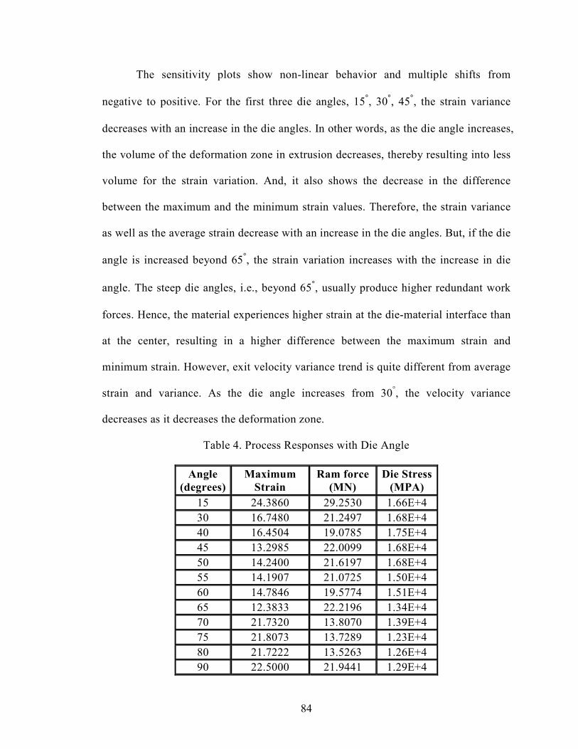
84
The sensitivity plots show non-linear behavior and multiple shifts from
negative to positive. For the first three die angles, 15°, 30
°, 45
°, the strain variance
decreases with an increase in the die angles. In other words, as the die angle increases,
the volume of the deformation zone in extrusion decreases, thereby resulting into less
volume for the strain variation. And, it also shows the decrease in the difference
between the maximum and the minimum strain values. Therefore, the strain variance
as well as the average strain decrease with an increase in the die angles. But, if the die
angle is increased beyond 65°, the strain variation increases with the increase in die
angle. The steep die angles, i.e., beyond 65°, usually produce higher redundant work
forces. Hence, the material experiences higher strain at the die-material interface than
at the center, resulting in a higher difference between the maximum strain and
minimum strain. However, exit velocity variance trend is quite different from average
strain and variance. As the die angle increases from 30±, the velocity variance
decreases as it decreases the deformation zone.
Table 4. Process Responses with Die Angle
Angle
(degrees)
Maximum
Strain
Ram force
(MN)
Die Stress
(MPA)
15 24.3860 29.2530 1.66E+4
30 16.7480 21.2497 1.68E+4
40 16.4504 19.0785 1.75E+4
45 13.2985 22.0099 1.68E+4
50 14.2400 21.6197 1.68E+4
55 14.1907 21.0725 1.50E+4
60 14.7846 19.5774 1.51E+4
65 12.3833 22.2196 1.34E+4
70 21.7320 13.8070 1.39E+4
75 21.8073 13.7289 1.23E+4
80 21.7222 13.5263 1.26E+4
90 22.5000 21.9441 1.29E+4
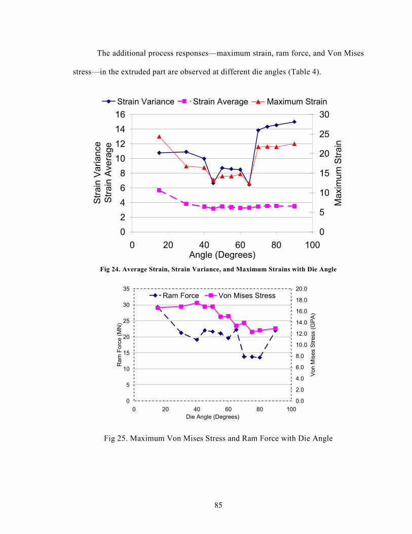
85
The additional process responses—maximum strain, ram force, and Von Mises
stress—in the extruded part are observed at different die angles (Table 4).
0
2
4
6
8
10
12
14
16
0 20 40 60 80 100Angle (Degrees)
Strain Variance
Strain Average
0
5
10
15
20
25
30
Maximum Strain
Strain Variance Strain Average Maximum Strain
Fig 24. Average Strain, Strain Variance, and Maximum Strains with Die Angle
0
5
10
15
20
25
30
35
0 20 40 60 80 100
Die Angle (Degrees)
Ram Force (MN)
0.0
2.0
4.0
6.0
8.0
10.0
12.0
14.0
16.0
18.0
20.0
Von Mises Stress (GPA)
Ram Force Von Mises Stress
Fig 25. Maximum Von Mises Stress and Ram Force with Die Angle

86
Average strain, variance, and maximum strains are plotted against die angles,
as shown in Fig. 24. The strain variance, Average strain, and the maximum strain
values decrease from an angle of 15° to 30
°, and thereafter show values until 60
±, and
then increase with die angle. However, the magnitudes of the changes are highly non-
linear and vary individually for the responses. At an angle of 65°, the strain variances
show minimum values that are apparently consistent with the sensitivities that are
plotted in Figs. 21-23, which depict the lowest sensitivity at die angle 65°. Thus, by
examining, it is possible to draw a near optimum die angle for the strain variance and
averages.
Von Mises stress and ram force are plotted against the die angle in Fig. 25.
The Von Mises stress curve initially shows an increasing trend with the die angle.
However, beyond a 45° die angle, the stress drastically decreases due to a decrease in
the deformation zone, and thereafter increases because of the higher frictional effects.
The ram force curve shows a distinct tendency from other responses. Unlike the other
responses, the ram force decreases even after a die angle of 60°. So, the near optimum
die angles for the other responses, i.e., strain variance and average strain, are not
necessarily the near optimum die angle for the total ram force. Thus, these
observations and computations provide a decent margin for different objective
functions and optimum design points.
4.5.6b. Sensitivities at Different Design Parameters
Furthermore, the novelty of the methodology is demonstrated by considering a
greater number of design variables. Six die shape coordinates (z1, r2, z2, r3, z3, z4) and
two fillet radii (fr1, fr2) are selected as design parameters, shown in Fig. 26. The

87
initial radius r1 and the final radius r4 are fixed; fr1 is the inlet fillet radius and the fr2
is the outlet fillet radius. The computed FDM and analytical sensitivities for the
objective functions strain variance and the average strain are tabulated in Table 5. The
differences between FDM and continuum sensitivities are very small.
Fig 26. Design Parameters (ri, zi)
θ
fr1+
+ fr2
– (ri, zi) r
z
ri
rf 1.322
1.191
1.059
0.928
0.796
0.665
0.534
0.402
0.271
0.440
0.086

88
Table 5. Objective Functions Sensitivities for Different Design Parameters
Sensitivities
Strain Variance Average Strain Design
Parameter FDM Analytical FDM Analytical
z1 -121.47 -121.36 2.35 2.35
r2 1369.52 1369.50 300.95 300.95
z2 185.07 185.02 66.13 66.13
r3 -105.71 -105.70 90.00 89.10
z3 -37.81 -37.81 11.71 11.71
z4 -60.89 -60.90 15.73 15.73
fr1 110.10 110.18 0.00 0.00
fr2 -180.00 -182.00 700.00 698.98
Here, the analytical and FDM sensitivities are consistent in both signs and
magnitudes. From the results, it can be seen that if the radius and the vertical
coordinate of the second point are increased, the steepness of the die increases and
results in an increase in the strain variance. Increasing the z1 basically decreases the
deformation length, thereby decreasing the strain variance. However, the average
strain is insensitive to change in z1 and holds small positive value. It can also be noted
that the increase in inlet radii increases the area of the die-material contact and
thereby increases the strain variation. However, it shows no change in the average
strain with zero sensitivity. The strain variance decreases with the increase in outlet
radius because this facilitates smooth flow of material and mitigates the high
frictional effects.
Thus, the developed sensitivities provide quantitative measurement for process
changes with respect to die shape parameters and also aid in reaching the optimum
design point. Moreover, the developed sensitivities can be utilized to screen the
critical process parameters. The parameters that show large sensitivity values are
considered as critical, whereas the parameters with relatively small values, such as

89
0.001, can be neglected in the design process. Additionally, design parameter
sensitivities can be utilized in trade-off cost studies, and reliability-based designs can
be used to achieve the required process performance.
It can also be noted that the number of simulations that are utilized to compute
analytical sensitivities are just two for a single objective function. Thus, the
developed sensitivity method significantly reduces the number of simulations for
problems with a large numbers of design parameters, thereby reducing the overall
computational cost required by optimization algorithms. Furthermore, the developed
sensitivity formulation can be easily incorporated in any existing commercial
software without changing the finite element formulations or needing source code of
the programs.

90
5. Design Optimization
In design optimization problems, evaluation of the objective function and
constraints requires the execution of costly metal forming finite element analyses for
velocities, strains, stresses, or other responses. The shape optimization process may
require that the objective function and constraints hundreds or thousands of times be
evaluated. The cost of repeating the finite element analysis is very high. However,
this computational cost problem can be addressed by the use of approximations
during the optimization process, as shown in Fig. 27. First, an exact analysis is
performed with an initial design and then the analytical sensitivity information (as
explained in Chapter 4) is computed. The original design problem is changed into a
sequential approximate optimization problem with an approximate representation of
objectives and constraints. Then, the approximate problem is solved by an
optimization algorithm. The objective function value is obtained at the optimum
solution and compared with the initial value. If the convergence requirement is not
satisfied, the process is repeated until convergence. Since the approximation has
replaced the expensive exact objective and constraint calculations, significant
computational savings can be achieved, particularly in conjunction with robust design
methodology (explained in Chapter 6). Hence, the research investigated function
approximation techniques that utilize analytical sensitivity information for shape
optimization.

91
Fig 27. Shape Optimization Procedure with Function Approximations
Die shape optimization consists of the following steps:
• Identifying and screening critical shape parameters
• Exploring the design space by Design Of Experiments
• Obtaining process performance values and their sensitivities at DOE points
• Constructing local approximation models
• Constructing global approximation
• Performing design optimization.
The design methodology starts by identifying the critical shape parameters that
affect the various forming process performances, product quality and reliability.
Extrusion die angle is the one of the most important parameters in angular die and
Compute objective and constraints
functions
Input data
Initial guess shape
Final desired performance criteria
Perform finite element analysis
Obtain state variables
Call optimization routine
New shape design
Optimum shape
Y
N
Continuum sensitivity analysis
• Utilize deformation mechanics • Formulate explicit sensitivity expression
Is design
satisfied? Function
Approximations

92
hence taken as critical shape parameter. Then factorial methods/DOE [Box et al.
1978] are used to create the design points over the design space. The responses of the
forming process, such as strain variance, average, and velocity variance are obtained
at different design points. Then, an approximation model, i.e. Two-Point Adaptive
Non-Linear Approximation, is constructed with the obtained responses at design
points. Thereafter local approximations are combined into multi-point approximation.
Then, die shape optimization is performed by using generated surrogate models. The
basic principles of DOE, approximations are presented in the following sections.
5.1. Design of Experiments
Design of experiments is the application of geometric principle to a statistical
sampling to obtain desired results such as minimizing the necessary number of
experiments, or minimizing the variance of estimate coefficients obtained through
regression. To generate approximation model, design of experiments at certain design
points are needed. Two-level, three-level, and five-level factorial designs are the broadly
used schemes of the design of experiment. The two-level factorial design is only suitable
for fitting the linear approximation models. To generate higher-order models, the design
variables usually should be tried at least three levels. The total number of experiments is
3k for the three-level factorial design, where k is the number of the design variables. For a
small number of design variables, the three-level factorial design is applicable. As the
number of design variables increase the design points grows rapidly. For example, with 6
design variables, the total number of experiments is 729 for three-level factorial designs.
By adding some additional points to two-level factorial design, the higher-order
approximation models can be effectively fitted.

93
Among all of the factorial methods, the Central Composite Design (CCD)
method offers a satisfactory alternative to a full factorial design.
Fig 28. Central Composite Design
A CCD (Fig. 28) contains an embedded factorial or fractional factorial design
with center points that are augmented with a group of ‘star points’ that allow
estimation of the curvature behavior of the system performance [Montgomery et al.
1997]. Hence, this method is used for selecting the design points in this research. The
total number of simulations required for the CCD method is 2k+2k+N, where k is the
number of parameters and N is the number of center points. At chosen design points,
the finite element analyses are conducted and the required performance values and
gradients are obtained over the design span. With these information Two-Point
Adaptive Non-linear Approximations are constructed locally. And these local
approximations are combined using Multi-Point Approximation weighting functions.
The details are provided in following sections.
5.2. Improved Two-Point Adaptive Non-Linear Approximation
Improved Two-Point Adaptive Non-Linear Approximation (TANA 2) has the
capability to match the nonlinearity of metal forming process response functions

94
[Wang et al. 1995]. Two-point approximation is constructed based on the function
values and gradients information of two points. One point is selected as the current
point and the other is the previous point. In TANA 2, intervening variables are used in
conjunction with Taylor series expansion and defined as
iP
ji xy = , i=1, 2, …, n (5-1)
where iP is the nonlinear index, which is different for each design variable. Taylor
series expansion at current point X2 is written as
( ) ( )( ) ( ) ( )∑∑
==
−
−+−∂
∂+=
n
i
p
i
P
i
n
i
P
i
P
i
i
P
i
i
iiii
i
xxxxP
x
x
XgXgXg
1
2
2,2
1
2,
1
2,22
2
1~ ε (5-2)
This approximation is a second-order Taylor series expansion in which the Hessian
matrix has only diagonal elements of the same value. This expression has n+1
unknown constants, so, n+1 equations are required. Differentiating the Equation (5-2),
n equations are obtained by matching the derivative with the previous point X1
derivative:
( ) ( ) ( ) i
P
i
P
i
P
i
i
P
i
i
i
Pxxxx
Xg
x
x
x
Xgiii
i
1
1,2,1,22
1
2,
1,1 −
−
−+∂
∂
=
∂
∂ε (5-3)
Another equation is obtained by matching the exact and approximate function values
with the previous point X1:
( ) ( )( ) ( ) ( )22,1,2
1
1
2,1,2
21 2
1
2, ii
i
iii P
i
P
i
i
Pn
i
P
i
P
i
i
xxP
xxx
x
XgXgXg −+
−
∂
∂+=
−
=
∑ ε (5-4)
There are many algorithms for solving these n+1 equations as simultaneous equations.
MATLAB adaptive search technique is used to solve the n+ 1 simultaneous equations.

95
5.3. Multi-Point Approximation
The multi-point approximation can be regarded as the connection of many local
approximations [Wang et al. 1996]. With function and sensitivity information already
available at a series of points, one local approximation is built at each point. All local
approximations are then integrated into a multi-point approximation by the use of a
weighting function. The weighting functions are selected such that the approximation
reproduces function and gradient information at the known data points.
If the function ( )XF and gradient ( )x
XF
∂
∂ information is available at
Tknkkk xxxX ,,2,1 ,,, L= where k = 1, 2, ..., K then the multi-point approximation can be
written in terms of the local approximations as,
( ) ( ) ( )∑=
=K
k
kk XFXWXF1
~~ (5-5)
where Wk is a weighting function, written as
( )( )
( )∑=
=K
j
j
k
k
X
XXW
1
φ
φ (5-6)
and ( )XF~
is a local approximation. ( )XWk adjusts the contribution of ( )XFk
~ to ( )XF
~in
Equation (5-5). ( )Xkφ is called a blending function and has its maximum of 1 at Xk and
vanishes when Xk is very far from X.
Several blending functions in equations (5-7, 8, and 9) can used to make the MPA
reproduce the exact function and gradient values at the data points, where the local
approximation was built. There are at least three blending functions that could meet this
requirement. They are:

96
( )( ) 1
1
−=
k
khExp
Xφ (5-7)
( )( )1log
1
+=
k
kh
Xφ (5-8)
and ( )k
kh
X1
=φ (5-9)
where ( )m
n
i
kiik xxh
−= ∑
=1
2
, (5-10)
where m is a positive integer. Additionally, it is recommended, from computational
consideration, that the design space be normalized as xi∈ [0, 1] to measure the weighting
function.
Each of the weighting function has the following properties:
( )kjjk XW δ= (5-11)
( ) 10 ≤≤ jk XW (5-12)
( )K
XWLim kx j
1=
±∞→ (5-13)
( ) 11
=∑=
K
k
k XW (5-14)
The weighting function varies between 0 and 1, and the summation of all weighting
functions is 1. The MPA is an average value of all the local approximation estimations
when a design point is far from every data point.
5.4. Optimization Problem
The optimization problem is formulated to minimize the exit velocity variance
of an axisymmetric extrusion problem. Die angle is considered as design variable.

97
Constraints are placed on the amount of strain variance and average strain. In this
case study, maximum strain variance is limited to 10.0 and maximum average strain is
limited to 3.3. These inequality constraints in its normalized domain can be
represented as
0.00.1s
s1 ≤−=
trainvar
trainvar
Desired
Actualg (5-15)
0.00.1s
s
2 ≤−=trainavg
trainavg
Desired
Actualg (5-16)
Table 6. TANA 2 Approximation Parameters
TANA 2 Points Velocity Variance Strain Variance Average Strain
Current Previous Pi values Epsilon Pi values Epsilon Pi values Epsilon
30 40 2.2855 0.44 1.3250 1.00 1.9005 1.00
40 45 -1.8764 -0.01 -4.5005 0.00 0.3890 0.04
40 50 -1.9574 -0.01 3.3154 0.10 3.9518 0.09
45 50 4.5000 0.500 -0.3090 0.51 -0.0130 1.00
45 55 3.3149 0.59 -0.3905 0.51 -0.0130 1.00
50 55 1.8120 0.53 0.3820 0.35 0.4550 0.15
50 60 -1.2565 0.61 4.5000 -1.00 4.2729 0.32
55 60 -1.7274 0.50 0.0855 0.34 0.0020 0.50
55 65 -1.3985 0.50 0.5740 0.13 0.0020 0.50
60 65 -0.3485 1.00 -1.7944 0.50 0.0860 1.00
60 70 -0.3585 1.00 -3.6338 0.01 1.7475 1.00
65 70 -4.0043 -0.02 0.8695 0.65 1.9140 1.00
65 75 -4.4720 -0.01 -0.0095 0.50 2.3649 1.00
70 75 2.7949 0.60 -0.0245 0.69 -0.0035 0.51
70 80 1.3340 0.53 -0.0190 0.91 -0.0035 0.50
75 80 1.9035 0.49 0.9340 0.83 0.0010 0.50
80 90 -4.5005 -0.28 4.5000 1.00 -0.006 -0.48
The objective and constraint functions are approximated using MPA methods.
The die angle design space is considered from 30± to 90
±. The design points, responses,
and sensitivities from Tables [1-3] are used to construct approximations. Local

98
approximations are constructed only if the two points are 10± apart. This distance
condition avoids the effect of distant local approximation and facilitates the capture of
variance locally. And then the non-linear indices Pi and error terms 2ε are computed
for each function, as in Table 6.
The MPA models for above mentioned objective and constraint functions
predict the responses accurately at sampled design points [Figs. 29-31] because a
maximum weight of 1 will be given to the TANA-2s constructed at that design point.
Hence, the predicted response exactly matches the actual response. However, the
responses at the last design point don’t match the actual response because there is no
TANA-2 constructed at the last design point.
0
5
10
15
20
25
30 40 45 50 55 60 65 70 75 80 90Die Angle
Velocity Variance
Original Val App Val
Fig 29. Velocity Variance Actual vs. Approximation Values

99
0
2
4
6
8
10
12
14
16
30 40 45 50 55 60 65 70 75 80 90
Angle (Degrees)
Strain Variance
Original Val App Val
Fig 30. Strain Variance - Actual vs. Approximation Values
2.8
2.9
3
3.1
3.2
3.3
3.4
3.5
3.6
3.7
3.8
3.9
30 40 45 50 55 60 65 70 75 80 90Angle (Degrees)
Strain Average
Original Val App Val
Fig 31. Average Strain - Actual vs. Approximation Values

100
Using the MPA models, the die shape optimization problem can be formulated
to minimize the objective function by subjecting to constraint functions. .
The optimization problem can be expressed mathematically as:
Objective: Minimize exit velocity variance ( )θψ (5-17)
Subject to:
( ) 0.01 ≤θg (5-18)
( ) 0.02 ≤θg (5-19)
oo 9030 ≤≤ θ (5-20)
The exit velocity variance, strain variance, and average strain are represented
using the MPA. These MPA equations are then used to find the optimum die angle.
Convergence history of optimization results is shown in Figs. 32 and 33.
0
10
20
30
40
50
60
70
80
90
100
0 5 10 15 20
Iteration Number
Die Angle
Fig 32. Design Variable Convergence History

101
0
2
4
6
8
10
12
14
16
0 5 10 15 20
Iteration Number
Exit Velocity Variance
Strain Variance
3.15
3.2
3.25
3.3
3.35
3.4
3.45
3.5
3.55
Strain Average
Objective -Exit Velocity Variance
Constrain1 - Strain Variance
Constraint 2 - Strain Average
Fig 33. Objective and Constraint Functions Convergence History
The metal forming processes is highly nonlinear and it gives multiple local
optimum values with different initial values. Among all, the optimum point which
gives the lowest objective function value is chosen as optimum design angle. The
initial angle for the optimization is chosen as 46± and after 15 iterations, the optimum
value is achieved. The optimum die angle is 58.97±. The constraint average strain is
obtained as 3.3, which is active at the optimum point. Strain variance is obtained as
8.5242, which is inactive.
However, all the above mentioned sensitivity and optimization techniques
assume that the design and process variables are deterministic in nature. But in
practice, there exists randomness in the process and operating conditions. These

102
variations often induce premature die failures and process break-downs. And they
also affect the final part geometry accuracy and productivity. Hence, these variations
should be considered in the design process. Lepadu et al. (2006) investigated
extrusion die wear under various process conditions variations. He studied die wear
variance with friction coefficient, extrusion ratio, and angle of the die as random
parameter. He used DOE and response surface method to find the main and
interaction effects. However, the study doesn’t develop design procedure in variable
situations. Hence, this research develops a robust die design methodology, which
considers the variations in design variables as well as process and operating
conditions. Uncertainty Quantification (UQ) and Reliability-Based Optimization
(RBDO) methods are utilized in the design process along with sensitivity analysis and
MPA techniques. The details of the robust design methodology, uncertainty
quantification techniques, and reliability-based optimization method are presented in
the following Chapter.

103
6. Robust Design
One of the primary goals of the forming industry is to assure proper levels of
product quality with reduced need for additional prototyping. This seemingly simple
task is complicated by the uncertainties that result from multiple parameters. Forming
process reliability and durability is dictated by the process performance in the
presence of uncertainties in various process and model parameters. In conventional
forming process optimization, the design is subjected to certain constraints associated
with manpower, material used, equipment capacity, and so on. Many optimization
techniques have been developed in order to satisfy these constraints. However,
traditional approaches have simplified the problem by considering the uncertainties
through empirical safety factors. These safety factors were derived based on
experience but do not guarantee safety or optimum performance. These approaches,
therefore, do not take into account any uncertainty related to the design parameters.
A process that is insensitive to variations in parameters is described as robust.
For instance, we may have a manufacturing process to make a product (e.g., metal
wheels), but despite our best efforts the product quality varies widely. This variation
occurs due to process parameters like ambient temperature, friction factor (due to
repeated use of lubricant), initial billet temperature (due to heat transfer that occurs in
transferring billet to dies from the furnace), ram velocity, and stroke length (due to
machine backlash errors). Rather than tightening up tolerances on the process

104
parameters, it may be advantageous to adjust the level of these parameters to reduce
their sensitivity, i.e., robust design under uncertainties. This way we end up with a
consistent high quality product.
Generally, uncertain parameter information can be obtained either as sparse
data points, intervals, expert opinions, or as probability distributions. Depending on
the uncertainty information available, it propagates from one step of the process or
discipline to another. Hence, this research developed a Robust Design Technique to
identify and quantify these parameter uncertainties by using reliability analysis tools,
uncertainty quantification and reliability-based optimization. Robust design
methodology of the forming process consists of the following steps:
• Identifying uncertainty parameter sources
• Screening critical parameters
• Evaluating the uncertainties and their probability distributions
• Variability assessment
• Reliability assessment
• Reliability-based optimization.
The forming process reliability and outcome depend on a number of
parameters like workpiece initial temperature, friction factor, stroke length, and ram
velocity. Among these parameters, critical parameters have to be identified, which is
done using Design of Experiments (DOE) techniques. MPA is generated with
function and sensitivity information at DOE points and used to represent the system
behavior. Variation in the system response is estimated by applying a Monte Carlo

105
Simulation (MCS) on the MPA. Cumulative Distribution Functions (CDF) are
generated to represent system variability. Process reliability is evaluated by
estimating the probability of failure and the safety index of the behavior. To make the
process robust, parameter uncertainties are considered in the optimization by applying
reliability constraints. Figure 34 depicts the overview of robust design methodology.
Fig 34. Robust Design Methodology
6.1. Possible Sources of Uncertainties
Uncertainties in the forming processes come from both quantitative and
qualitative sources. Quantitative or non-cognitive sources are related to randomness
in physical observations, which come from variations in process conditions, such as
randomness in friction factor, ram velocity variations, stroke length variations, and
billet temperature variations. Qualitative or cognitive sources are related to skill or
experience of the operator and the conditions of the machinery. The forming system
can be visualized as a system with a large number of interacting random parameters
and sources as shown in Fig. 35.
Uncertainty quantification
Variability assessment
Reliability assessment
Reliability-Based
Optimization
• Screen critical parameters
• Evaluation of uncertainties
Most probable failure point
† Probability of failure
† Reliability index
† Probability distribution function
† Cumulative distribution
function

106
Fig 35. Interaction among State Variables and Uncertainty Sources
Depending on the nature of the sources, the uncertainties in forming processes can be
classified into four categories [Repalle et al. 2005]. They are:
• Die/workpiece-based uncertainties
• Material-based uncertainties
• Process and model parameter uncertainties
• Other miscellaneous uncertainties
Die/Workpiece-Based Uncertainties: These uncertainties include variations related
to die/workpiece such as variations in workpiece initial shape inconsistencies, heating
times, die and die temperature profiles, workpiece transferring times from the furnace
to the die, and alignment positions.
Billet / die
temperatures Friction factor Die velocity Stroke
length
Underfill
Flash Temperature
distribution
Flow stress
Formability
Strain
• Metal flow
• Forming load
• Energy
• Product quality
• Die life
Die / die shape
• Human error • Assembly Errors • Tool wear
• Lubrication system • Interface temperatures • Type of lubrication
Dimensional
tolerances
Heat transfer from • Billet to die • Billet to atmosphere • Die to atmosphere

107
Material-Based Uncertainties: These uncertainties consist of variations in
workpiece and die material compositions, microstructure, elastic, plastic, and thermal
properties.
Process and Model Parameter Uncertainties: There exist uncertainties in process
and model parameters, such as friction coefficients at the interface, heat transfer rates,
and stroke lengths, due to repetitive use of lubrication, inconsistent cooling rates, and
machinery fatigue conditions. These uncertainties also arise from variations in
lubrication system, i.e., spray angle, time, pattern, and speed and heat treatment
process.
Other Miscellaneous Uncertainties: Errors in tooling assembly, human intervention,
and environmental conditions such as temperature and humidity are some of the other
miscellaneous uncertainties.
6.2. Screening of Critical Parameters
This research focuses on some of the quantitative random parameters. Based
on the considerations given in manufacturing industry, the following representative
random parameters are considered: operational parameter–ram velocity, process
parameter–friction factor, and material parameter–strain-rate sensitivity index (n).
These parameters strongly influence the mechanical behavior of the deforming
material and have a direct impact on the spatial and temporal distribution of state
variables like Von Mises stress, effective strain variance, exit velocity variance, and
total load.
Factorial screening methods are used to identify each random parameter’s
contribution to the response of the extrusion system. The sensitivity of each parameter

108
for the response is analyzed through ANalysis Of VAriance (ANOVA) and DOE
analyses. Using a two-level fractional factorial DOE, the simulation points are
generated. The strain variance, average strain, exit velocity variance, and extrusion
forming load, for each DOE design point is computed and the main effect of each
process parameter is evaluated. Together, the analyses yield Pareto plots as shown in
Fig. 36, and enable the identification of critical variables.
0
0.1
0.2
0.3
0.4
0.5
0.6
0.7
Strain Variance Strain Average Exit Velocity
Variance
Forming Load
Performance
Parameters Relative Effect
Friction Factor Ram Velocity S-R Index
Fig 36. Pareto Plot Process Performance
From the Pareto plot, it is shown that the friction factor and ram velocity
together contribute 80-95% of the overall response to strain variance, average, and
exit velocity variance. Strain-rate sensitivity index (S-R index) contributes 20% in
forming load. But, the focus is on reducing the geometric distortions and local strain
concentrations in the extruded part, responses strain variance, average, and exit

109
velocity variances are considered further in the optimization. Hence, the most
influential parameters friction factor and ram velocity are chosen as random
parameters. These parameters are defined with probability distributions.
6.3. Probability Distributions
Probability distributions are typically defined in terms of the Probability
Density Function (PDF). However, there are number of probability functions used for
random parameters. The selection of a particular type of probability distribution
depends on the following factors:
• Available format of the data
• The nature of the problem
• The underlying assumptions associated with the distribution
• Convenience and simplicity for further computations
The properties of some of the most commonly used distributions [Haldar et al.
2000] are Normal, Standard Normal, Lognormal, Gamma distributions, etc.
6.3.1. Normal Distribution
Normal distribution (also known as Gaussian distribution) is a symmetric and
bell-shaped density curve for a random parameter. The normal distribution is
characterized by two parameters: the mean µ and the standard deviation σ. The mean
is a measure of center and the standard deviation is a measure of spread. The density
function of the normal distribution is given by the equation (6-1)
−−=
2
50exp2
1
σ
µx.
σπf (6-1)

110
Here x is random variable and can take any value from -∞ to +∞. The normal PDF of
a random parameter is shown in Fig. 37. The normal distribution has the following
properties:
• The linear function of normal random variables is also normally distributed.
• The non-linear function of normal random variables can be normal, weibull,
gamma, lognormal, etc.
Fig 37. Notmal Distribution
6.3.2. Standard Normal Distribution
A Gaussian distribution with parameters mean µ=0 and the standard deviation
σ=1 is called a standard normal distribution. It is identified as N(0,1). The probability
density function of standard normal variable x is given by equation (6-2)
−=2
exp2
1 2x
πf (6-2)
The distribution is symmetric about mean µ = 0 as shown in Fig. 38.
x
σ
µ
Pro
bability D
ensity F
unction

111
Fig 38. Standard Normal Distribution
6.3.3. Lognormal and Gamma Distributions
A random variable x is said to follow lognormal distribution if y = ln(x) and
follows normal distribution. Thus, the density function can be written as:
−−=
2
50exp2
1
σ
µy.
σπf (6-3)
where y = ln(x) and -∞ < y < ∞.
The gamma distribution consists of the gamma function, a mathematical
function defined in terms of an integral. The density function of the gamma
distribution is defined as
( )
0
01 1
≥
=
−−
therwise O
xexαΓβf
xα
α (6-4)
where parameters α and β satisfy α > 0, β > 0, and Γ(α) is gamma function.
x σ µ = 0
Pro
bability D
ensity
-σ

112
6.3.4. Cumulative Distribution Function
The Cumulative Distribution Function (CDF) is the probability that the
variable takes a value less than or equal to x. For a continuous function, it can be
expressed as
∫ ∞−=
x
f(x)dxF (6-5)
Where f(x) is the probability density function, the CDF plot for a normal variable is
shown in Fig. 39. The y-axis represents the probability and the horizontal axis is the
allowable domain for the given probability function.
Fig 39. Normal CDF
6.4. Response Variability
In practice, the distribution and correlation between parameters depends on the
available information. Here in this research, random parameters are assumed as
independent to each other and follow Gaussian distribution with 10% variance. The
cumulative effect of all these distributions causes the overall probability distribution
of the response function. After the MPA is developed for the system performance or
0
1
Pro
bability
x

113
objective, the effect of uncertain parameters can be incorporated into the model
through the use of Monte Carlo Simulations (MCS). MCS is, effectively, a random
number generator that creates values for each uncertain parameter. Values are chosen
within the limits for each variable and with a frequency proportional to the shape of
the probability distribution associated with each variable. A response value is
computed for each occurrence of the parameter using MPA. System response
variability is then represented through PDF and CDF.
6.5. Reliability Index
Process reliability is the probability that a system can perform its intended
function for a specified interval under specified conditions. Generally, reliability
analysis uses the limit state function to evaluate the probability of process failure by
determining whether the limit state functions are greater or less than zero. One of the
limit state functions in forming is the exit velocity variance function, which can be
written as
( ) SRxg −= =limit exit velocity variance – actual exit velocity variance (6-6)
Here the variance is a MPA, a function of random parameters. The limit state
function g(x) = 0 is the boundary between safe and unsafe process. The failure of the
process occurs if the actual variance exceeds the limit variance. Hence, probability of
failure is defined as
Pf = P [g(x) < 0] (6-7)
It is computed as the integration of the joint probability density function over failure
region; mathematically it is written as
dSdRfPΩ
RSf ∫= (6-8)

114
fRS is joint probability density function. Ω is failure region, i.e., g(x) ≤ 0. Pf can also
be mentioned with the use of a standard normal cumulative distribution function as
follows:
Pf = Φ(β) (6-9)
where Φ standard normal cumulative density function and β is the reliability index. β
is the minimum distance from origin to design point on limit state surface as shown in
Fig. 40 [Haldar et al. 2000]. This minimum distance point is called the “Most
Probable Failure Point” (MPP). MPP represents the worst combination of stochastic
variables with the highest probability of failure.
Fig 40. Reliability Index
For non-linear limit state functions, the computation of the β becomes an
iterative optimization problem and is described as follows:
Objective: Minimize XXβ T=
Subject to Constraint g(X) = 0
MPP
β
g(x) > 0
Safe
g(x) < 0
Unsafe
Limit State g(x) = 0
0
X2
X1

115
where X is the coordinate vector of MPP. They represent the magnitude of design
variables
Thus, the calculated probability of failure will be used as random constraints
in the optimization problem, called Reliability-Based Optimization.
6.6. Reliability-Based Optimization
In deterministic-based extrusion die shape optimization (Chapter 5), the
random parameters friction factor and ram velocity are assumed to constants to their
mean values, 0.3 and 50 mm/sec. However, they vary in general manufacturing
process. In reliability analysis, this variation is accounted by assigning normal
probability distribution with 10% standard deviation. Extrusion die angle is design
variable (explained in previous Chapters 4 & 5). Using the CCD method,
experimental points are designed for design and random parameters. After designing
the experimental points, the next step is to obtain the objective and constraint function
distribution in the presence of random parameters. The number of random parameters
in this example is two. They are: friction factor and ram velocity. Forming
simulations are conducted at these DOE points. Strain variance, average, and exit
velocity variance are obtained from FEA simulation for every experimental point.
Then, MPA are fitted to each response in terms of design and random parameters. All
the random parameters are assumed independent to each other. Then MCS is applied
on generated MPA, and response variability distribution is obtained. Thus, for every
design point, response variability PDF is obtained. The constraint functions’
probabilities of failures are computed. As in earlier optimization (Chapter 5), strain
variance limit 10.0 and average strain limit 3.3 are used to construct limit state

116
functions. The mean, standard deviation, and probability of failure are computed from
the MPA approximation models. Using these means and probabilities, an optimization
is formulated. The reliability-based optimization problem mathematically can be
written as
Objective: Minimize Mean of exit velocity variance ( )( )θψµ (6-10)
Subject to:
( )[ ] 01.00.01 ≤−≤θgPf (6-11)
( )[ ] 01.00.02 ≤−≤θgPf (6-12)
oo 9030 ≤≤ θ (6-13)
Here, ( )θ1g is strain variance limit state function and ( )θ2g is average strain
limit state function. The approximation equations are then optimized using MATLAB
optimization tool box. Optimization is performed with different starting points. Table
7 tabulates starting and optimum points and the objective and constraint function
values.
Table 7. Optimum Points with Different Starting Points
Starting
point (deg)
Optimum
point (deg)
Objective
Exit velocity
variance
Constraint 1
Pf (strain
variance)
Constraint 2
Pf (average
strain)
46 45.425 2.9145 0.0222 0.0011
50 50.000 5.8536 0.0133 0.0055
55 55.137 4.7473 0.0011 0.0011
60 61.075 4.3833 0.0011 0.0733
65 65.000 3.3766 0.0710 0.2242
In this selected problem, objective function and constraints values vary in
nonlinear nature. They have multiple maximums and minimums. Multiple starting

117
points give resultant local optimums as shown in Table 7. Among all of the possible
local optimum points, 45.425± gives minimum objective function value. Hence, this
angle is selected as optimum die angle. After 20 iterations optimum point is achieved.
Convergence history of optimization is shown in Figs. 41 and 42.
39
40
41
42
43
44
45
46
47
0 5 10 15 20 25 30
Iteration Number
Die Angle (Deg)
Design Variable
Fig 41. Design Variable Convergence
0
2
4
6
8
10
12
14
0 10 20 30
Iteration Number
Exit Velocity Variance
0
0.01
0.02
0.03
0.04
0.05
0.06
0.07Probability of Failures
Strain Variance
Average Strain
Objective Constraint 1 Constraint 2
Fig 42. Objective and Constraint Functions Convergence
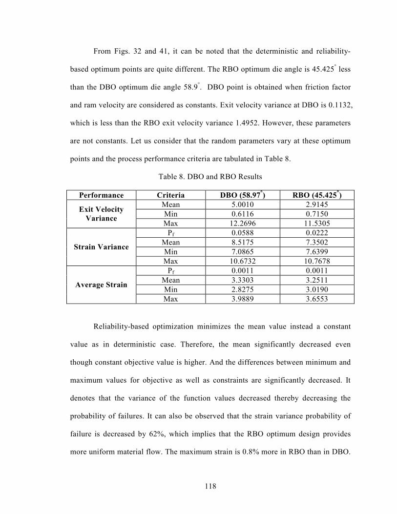
118
From Figs. 32 and 41, it can be noted that the deterministic and reliability-
based optimum points are quite different. The RBO optimum die angle is 45.425± less
than the DBO optimum die angle 58.9±. DBO point is obtained when friction factor
and ram velocity are considered as constants. Exit velocity variance at DBO is 0.1132,
which is less than the RBO exit velocity variance 1.4952. However, these parameters
are not constants. Let us consider that the random parameters vary at these optimum
points and the process performance criteria are tabulated in Table 8.
Table 8. DBO and RBO Results
Performance Criteria DBO (58.97∞) RBO (45.425
∞)
Mean 5.0010 2.9145
Min 0.6116 0.7150 Exit Velocity
Variance Max 12.2696 11.5305
Pf 0.0588 0.0222
Mean 8.5175 7.3502
Min 7.0865 7.6399 Strain Variance
Max 10.6732 10.7678
Pf 0.0011 0.0011
Mean 3.3303 3.2511
Min 2.8275 3.0190 Average Strain
Max 3.9889 3.6553
Reliability-based optimization minimizes the mean value instead a constant
value as in deterministic case. Therefore, the mean significantly decreased even
though constant objective value is higher. And the differences between minimum and
maximum values for objective as well as constraints are significantly decreased. It
denotes that the variance of the function values decreased thereby decreasing the
probability of failures. It can also be observed that the strain variance probability of
failure is decreased by 62%, which implies that the RBO optimum design provides
more uniform material flow. The maximum strain is 0.8% more in RBO than in DBO.

119
And the mean strain variance decreased by 13% in RBO. More importantly, decrease
in exit velocity variance gives that the defects formation due geometric inaccuracies
will be decreased. Hence, we can achieve cost savings by reducing the rejection
percentage in production. Not only that, the higher product quality can be achieved
with reduced probability of failures. Thus, reliability-based optimization not only
reduces failure probabilities but also aids in achieving better quality and highly
reliable robust designs.

120
7. Summary
In this research, a rigorous, efficient sensitivity analysis approach for steady-
state forming processes is developed.
• The developed method utilizes continuum deformation equations, unlike
the traditional discrete approach.
• Material derivatives and the adjoint method are the tools that are employed
in the derivation of the formulation. The derived sensitivity formula ends
in terms of a boundary integral. Hence, there is no need to evaluate whole
domain variation vectors, which simplifies the computational effort.
• The computed sensitivities are utilized in trade-off designs and
optimization.
This research also focuses on developing non-traditional robust die shape
optimization concepts to include uncertainties in the process. The important aspects
are identification of critical random parameters and their distributions. A robust
design methodology is developed by combining the design sensitivity analysis with
random parameters. This allows quantification of the uncertainties and leads to
estimating the variability of the system.
• A cost effective reliability-based optimization techniques is developed by
utilizing multi-point approximations and analytical sensitivities.

121
• Monte Carlo simulations are used to compute probabilistic objective and
constraint functions. This methodology is implemented on an axisymmetric
extrusion.
• The die optimization problem is solved to minimize the exit velocity
variance while constraints are placed on strain variance and average strain.
From the results, it is shown that the reliability design decreases mean value of
exit velocity variance by 41%, which improves final part dimensional accuracy
significantly. And the reliability-based optimum die provides a more uniform material
flow thereby reducing the probability of failure. Therefore, this reliability-based
optimization reduces manufacturing risk and improves product quality and gives a
more accurate and robust optimum point than the deterministic-based solution. It is
also determined that if the forming process is designed by considering the
uncertainties, then fluctuations in process performances can be greatly reduced,
thereby improving the tool life and reliability.

122
8. Future Directions
As mentioned earlier, boundary integral methods have not been investigated
for metal forming problems. Due to their proven computational efficiency in
structural problems, the current research adopted their material derivative and
continuum principles and developed a sensitivity analysis technique for steady-state
metal forming processes. The current formulation utilizes Eulerian framework, in
which the mesh remains constant through out the simulation. In non-steady processes,
Lagrangian framework is used in which the mesh changes with shape change.
Therefore, we need to investigate the method of incorporating shape changes into the
sensitivity derivation. Lagrangian definitions should be considered for state variables
such as strain and strain-rate. It is also important to increase dimensionality of the
formulation in order to solve large-size three-dimensional problems.
The random parameters such as friction factor, ram velocity, and material
constitutive law constants are considered as deterministic values during sensitivity
derivation. Their variation is accounted by constructing multi-point approximations
and by employing Monte Carlo simulations on them. However, it is important to
incorporate their standard deviation during the sensitivity derivation to improve
accuracy and robustness of the formulation.
In this work, process random parameter variation is assumed as probability
distributions. In practice, the uncertainties can be in the forms of intervals, fuzzy

123
variables, and other distributions. Hence, more uncertainty quantification theories
should be investigated, especially for metal forming processes.

124
9. Bibliography
1. ABAQUS Analysis User’s Manual, ABAQUS Inc., Version 6.5, 166 Valley Street,
Providence, RI 02909, 2004.
2. Acharjee S., and Zabaras N., “The Continuum Sensitivity Method for the
Computational Design of Three-Dimensional Deformation Processes,” Computer
Methods in Applied Mechanics and Engineering, 2006 (in press).
3. Antunez H. J., and Kleiber M., “Sensitivity Analysis of Metal Forming Processes
involving Frictional Contact in Steady State,” Journal of Materials Processing
Technology, Vol. 60, No. 1 – 4, 1996, pp. 485 – 491.
4. Antunez H. J., and Kleiber M., “Sensitivity of Forming Processes to Shape
Parameters,” Computer Methods in Applied Mechanics and Engineering, Vol. 137,
1998, No. 3 – 4, pp. 189 – 206.
5. Arif A. F., “On the Use of Non-Linear Finite Element Analysis in Deformation
Evaluation and Development of Design Charts for Extrusion Processes,” Finite
Elements in Analysis and Design, Vol. 39, 2003, pp. 1007 – 1020.
6. Arif A. M., Sheikh A. K., and Qamar S. Z., “A Study of Die Failure Mechanisms
in Aluminum Extrusion,” Journal of Materials Processing Technology, Vol. 134,
2003, pp. 318 – 328.

125
7. Box E. P., and Hunter J. S., Statistics for Experiments, John Wiley & Sons, Inc.,
New York, 1978.
8. Choi K. K., and Huag E. J., “Shape Design Sensitivity Analysis of Elastic
Structures,” Journal of Structural Mechanics, Vol. 11, No. 2, 1983, pp. 231 – 269.
9. Choi K. K., and Seong H. G., “A Domain Method for Shape Design Sensitivity
Analysis of Built-Up Structures,” Computer Methods in Applied Mechanics and
Engineering, Vol. 57, 1986, pp. 1 – 15.
10. Choi J. H., and Kwak B. M., “Boundary Integral Equation Method for Shape
Optimization of Elastic Structures,” International Journal for Numerical Methods
in Engineering, Vol. 26, 1988, pp. 1579 – 1595.
11. Choi J. H., Won J. H., and Yoon J. M., “Boundary Method for Shape Design
Sensitivity Analysis in the Optimization of Three-Dimensional Elasto-Statics,” 6th
World Congresses of Structural and Multidisciplinary Optimization, Rio-de
Janeiro, Brazil, May 30 - June 03, 2005.
12. Chung K., and Hwang S. M., “Application of a Genetic Algorithm to the Optimal
Design of the Die Shape in Extrusion,” Journal of Materials Processing
Technology, Vol. 72, 1998, pp. 69 – 77.
13. Chung K., and Hwang S. M., “Application of a Genetic Algorithm to Process
Optimal Design in Non-Isothermal Metal Forming,” Journal of Materials
Processing Technology, Vol. 80 – 81, 1998, pp. 136 – 143.

126
14. Chung K., and Richmond O., “Ideal Forming – II: Sheet Metal Forming with
Optimum Deformation,” International Journal of Mechanical Sciences, Vol. 34,
No. 8, 1992, pp. 617 – 633.
15. Chung S. H., Fourment L., Chenot J. L., and Hwang S. M., “Adjoint State Method
for Shape Sensitivity Analysis in Non-Steady Forming Applications,”
International Journal for Numerical Methods in Engineering, Vol. 57, No. 10,
2003, pp. 1431 – 1444.
16. Dems K., “Sensitivity Analysis in Thermal Problems – II: Structure Shape
Variation,” Journal of Thermal Stresses, Vol. 10, 1987, pp. 1 – 16.
17. Gradhi R. V., “Computer-Aided Optimization for Improved Process Engineering
Productivity of Complex Formings,” Chapter 25, Multidisciplinary Process
Design and Optimization, July 2003, pp. 368 – 376.
18. Grandhi R. V., Kumar A., Chaudary A., and Malas J., “State-Space
Representation and Optimal Control of Non-linear Material Deformation using the
Finite Element Method,” International Journal of Numerical Methods in
Engineering, Vol. 36, No. 12, 1993, pp. 1967 – 1986.
19. Gao Z. Y., and Grandhi R. V., “Sensitivity Analysis and Shape Optimization for
Die Design in Thermo-Mechanical Coupled Analysis,” International Journal for
Numerical Methods in Engineering, Vol. 45, 1999, pp. 1349 – 1373.
127
20. Haldar A., and Mahadevan S., Reliability Assessment using Stochastic Finite
Element Analysis, John Wiley & Sons, Inc., 2000.
21. Han C. S., Grandhi R. V., and Srinivasan R., “Optimum Design of Forming Die
Shapes Using Non-Linear Finite Element Analysis,” American Institute of
Aeronautics and Astronautics Journal, Vol. 31, 1993, pp. 17 – 24.
22. Hardee E., Chang K. H., Tu J., Choi K. K., Grindeanu I., and Yi X., “A CAD-
based Design Parameterization for Shape Optimization of Elastic Solids,”
Advances in Engineering Software, Vol. 30, 1999, pp. 185 – 199.
23. Haug E. J., Choi K. K., and Komkov V., Design Sensitivity Analysis of Structural
Systems, Academic Press, New York, 1986.
24. Hwang S. M., and Kobayashi S., “Die Design in Shell Nosing at Elevated
Temperatures,” International Journal of Machine Tool Design, Vol. 27, No. 1,
1987, pp. 1 – 14.
25. Joun M. S., and Hwang S. M., “Die Shape Optimal Design in Three-Dimensional
Shape Metal Extrusion by the Finite Element Method,” International Journal for
Numerical Methods in Engineering, Vol. 41, 1998, pp. 311 – 335.
26. Kang B. K., Kim N., and Kobayashi S., “Computer-Aided Die Design in Forming
of an Airfoil Section Blade,” International Journal of Machine Tools and
Manufacturing, Vol. 30, 1990, pp. 43 – 52.

128
27. Kim N. H., Young K., and Choi K. K., “Meshfree Analysis and Die Shape Design
of Extrusion Process,” AIAA-2002-5563, Vol. 2002, pp. 1 – 10.
28. Kobayashi S., Oh S. I., and Altan T., Metal Forming and Finite Element Method,
Oxford University Press, 1989.
29. Lanka S. S., Srinivasan R., and Grandhi R. V., ”A Design Approach for
Intermediate Die Shapes in Plane Strain Formings,” ASME Journal of Material
Shaping Technology, Vol. 9, 1991, pp. 193 – 205.
30. Lee E. H. and Mallet R. L., “Stress and Deformation Analysis of the Metal
Extrusion Process,” Computer Methods in Applied Mechanics and Engineering,
Vol. 10, 1977, pp. 339 – 353.
31. Lee S. R., and Yang Y. D., “Shape Optimization of Flow Guides in Three-
Dimensional Extrusion Processes by an Approximation Scheme based on State
Variable Linearization,” International Journal for Numerical Methods in
Engineering, Vol. 66, 2006, pp. 1691 – 1716.
32. Lin A., Juchen X., Xinyun W., and Guoan H., “Optimization of Die Profile for
Improving Die Life in the Hot Extrusion Process,” Journal of Materials
Processing Technology, Vol. 142, 2003, pp. 659 – 664.
33. Lotfi A., “Optimal Shape Design for Metal Forming Problems by Finite Element
Method,” Proceedings in Applied Mathematics and Mechanics, Vol. 5, 2005, pp.
429 – 430.

129
34. MATLAB: User’s Guide, The MathWorks Inc., 24 Prime Park Way, Natick, MA
01760, 1999.
35. Mehta B.V., Ghulman H., and Gerth R., “Extrusion Die Design: A New
Methodology of Using Design of Experiments as a Precursor to Neural
Networks,” Journal of Materials, Vol. 51, No. 9, 1999.
36. Meric R. A., “Shape Design Sensitivity Analysis for Non-Linear Anisotropic Heat
Conducting Solids and Shape Optimization by the BEM,” International Journal
for Numerical Methods in Engineering, Vol. 26, 1988, pp. 109 – 120.
37. Montgomery, D.C., Design and Analysis of Experiments, John Wiley & Sons, Inc.,
New York, 1997.
38. Nanhai H., and Kezhi L., “Numerical Design of the Die Land for Shape
Extrusion,” Journal of Materials Processing Technology, Vol. 101, 2000, pp. 81 –
84.
39. Oh S. I., “Finite Element Analysis of Metal Forming Processes with Arbitrary
Shaped Dies,” International Journal of Mechanical Sciences, Vol. 24, No. 8, 1982,
pp. 479 – 493.
40. Park J. J., Rebelo N., and Kobayashi S., “A New Approach to Die Design in Metal
Forming with Finite Element Method,” International Journal of Machine Tool
Design, Vol. 23, 1983, pp. 71 – 99.

130
41. Pietrzyk M., Zmudzki A., Szeliga D., and Kuziak R., “Sensitivity of Parameters of
Forward-Backward Extrusion Test on Material Properties and Friction,” MS&T
Conference Proceedings, 2004, pp. 403 – 408.
42. Repalle J., and Grandhi R. V., “Design of Forging Process Variables under
uncertainties,” Journal of Materials Engineering and Performance, Vol. 14, No. 1,
Feb 2005, pp. 123 – 131.
43. Repalle J., and Grandhi R. V., “Reliability-Based Preform Shape Design in
Forging,” Communications in Numerical Methods in Engineering, Vol. 21, No. 11,
3 Jun 2005, pp. 607 – 617.
44. Schenk O., and Hillman M., “Optimal Design of Metal Forming Die Surfaces with
Evolution Strategies,” Computers and Structures, Vol. 82, 2004, pp. 1695 – 1705.
45. Smith D. E., “Design Sensitivity Analysis and Optimization for Polymer Sheet
Extrusion and Mold Filling Processes,” International Journal for Numerical
Methods in Engineering, Vol. 57, 2003, pp. 1381 – 1411.
46. Ulysse P., “Extrusion Die Design for Flow Balance using FE and Optimization
Methods,” International Journal of Mechanical Sciences, Vol. 44, 2002, pp. 319 –
341.
47. Wang, L. P. and Grandhi, R.V., “Improved Two-point Function Approximation
for Design Optimization,” AIAA Journal, Vol. 32, No. 9, 1995, pp. 1720 – 1727.

131
48. Wang L., and Grandhi R. V., “Multi-Point Approximations: Comparisons Using
Structural Size, Configuration, and Shape Design,” Journal of Strucutral
Optimization, Vol. 12, No. 2/3, October 1996, pp. 177 – 185.
49. Wifi A. S., Shatla M. N., amd Hamid A. A., “An Optimum-Curved Die Profile for
the Hot Forward Rod Extrusion Process,” Journal of Materials Processing
Technology, Vol. 73, 1998, pp. 97 – 107.
50. Zhao G., Wright E., and Grandhi R. V., “Forming Die Design with Shape
Complexity Control in Simulating Backward Deformation,” International Journal
of Machine Tools and Manufacturing, Vol. 35, No. 9, 1995, pp. 1225 – 1239.
51. Zhao G., Wright E., and Grandhi R. V., “Computer Aided Die Design in Forming
using the Inverse Die Contact Tracking Method,” International Journal of
Machine Tools and Manufacturing, Vol. 36, No. 7, 1996, pp. 755 – 769.
52. Zhao G., Huff, R., Hutter A., and Grandhi R. V., “Sensitivity Analysis Based Die
Shape Design Using the Finite Element Method,” Journal of Materials
Engineering and Performance, Vol. 6, No. 3, June 1997, pp. 303-310.
53. Zhao G., Wright E., and Grandhi R. V., “Sensitivity Analysis Based Die Shape
Design for Net-Shape Forming,” International Journal of Machine Tools
Manufacturing, Vol. 37, No. 9, 1997, pp. 1251 – 1271.


![Robust Stability Condition and Analysis on Steady …based on regular linear system theory. Li and Tsao [5] addressed the analysis and synthesis of robust stability and robust performance](https://static.fdocuments.in/doc/165x107/5f10561d7e708231d4489b42/robust-stability-condition-and-analysis-on-steady-based-on-regular-linear-system.jpg)


