Robust Semi-active Control of Aircraft Landing Gear System … · · 2014-03-30Robust Semi-active...
153
Robust Semi-active Control of Aircraft Landing Gear System Equipped with Magnetorheological Dampers Ajinkya A. Gharapurkar A thesis in The Department of Mechanical and Industrial Engineering Presented in Partial Fulfillment of the Requirements For the Degree of Master in Applied Sciences (Mechanical Engineering) at Concordia University Montreal, Quebec Canada “© Ajinkya A. Gharapurkar, 2014” “March 2014”
Transcript of Robust Semi-active Control of Aircraft Landing Gear System … · · 2014-03-30Robust Semi-active...
Robust Semi-active Control of Aircraft Landing Gear System Equipped
with Magnetorheological Dampers
Ajinkya A. Gharapurkar
A thesis
in
The Department
of
Mechanical and Industrial Engineering
Presented in Partial Fulfillment of the Requirements
For the Degree of Master in Applied Sciences (Mechanical Engineering) at Concordia University
Montreal, Quebec Canada
“© Ajinkya A. Gharapurkar, 2014”
“March 2014”
CONCORDIA UNIVERSITY
School of Graduate Studies
This is to certify that the thesis prepared
By: Ajinkya A. Gharapurkar
Entitled: Robust Semi-active Control of Aircraft Landing Gear System Equipped
with Magnetorheological Dampers
and submitted in partial fulfillment of the requirements for the degree of
Master in Applied Sciences (Mechanical Engineering)
complies with the regulations of the University and meets the accepted standards with
respect to originality and quality.
Signed by the final examining committee:
_____________________________________ Chair
______________________________________ Examiner
______________________________________ Examiner
______________________________________ Supervisor
______________________________________ Co-Supervisor
Approved by ________________________________________________
MAsc Program Director,
Department of Mechanical and Industrial Engineering
________________________________________________
Faculty of Engineering and Computer Science
Date ________________________________________________
Dr. I. Contreras
Dr. S. Williamson
Dr. I. Stiharu
Dr. R. Bhat
Dr. C. Asthana
Dr. S. Narayanswamy
Dean Christopher Trueman
III
ABSTRACT
Robust Semi-active Control of Aircraft Landing Gear System Equipped with
Magnetorheological Dampers
Ajinkya A. Gharapurkar
Landing is the most critical operational phase of an aircraft since it directly affects the
passenger safety and comfort. The factors such as the undesirable wind and ground
effects, runway unevenness, excessive sink speeds and approach speeds and pilot errors
can deteriorate the landing performance of an aircraft several times during its entire
lifetime. When an aircraft lands, large amplitude vibrations get transmitted to the fuselage
from the runway thereby causing safety and comfort problems and hence need to be
suppressed quickly.
Landing gear is an essential assembly that prevents the aircraft fuselage from the
ground loads. A shock absorber which is considered as the heart of the landing gear
assembly plays an important role in this process by absorbing the vibrations during
landing. The existing Oleo-pneumatic shock absorbers are the most efficient in absorbing
the vibrations during each aircraft operation. However, they are unable to provide the
continuously variable damping required during the landing phase which might reduce
their efficiency. Moreover, to account for the uncertainties during landing, a damper
capable of providing the variable damping effect can play a vital role in increasing the
passenger safety.
A semi-active control system of a landing gear suspension can solve the problem
of excessive vibrations effectively by providing a variable damping during each
IV
operational phase. Magnetorheological (MR) dampers are one of the most efficient and
attractive solutions that can provide the continuously variable damping required
depending on a control command.
This thesis focuses on the concept of the semi-active aircraft suspension system
using the MR damper with the implementation of robust control strategy. Initially, the
dynamic behavior of the MR damper is studied using the parametric modeling approach.
Spencer dynamic model is adopted for simulating the dynamic behavior of the MR
damper. This is followed by the analysis of the energy dissipation patterns of the MR
damper for different excitation inputs.
A semi-active suspension system is developed for a three degree-of-freedom (3
DOF) aircraft model considering a tri-cycle landing gear configuration. A switching
technique is developed in the simulation of the landing procedure which enables the
system to switch from the single degree of freedom to three degrees of freedom system in
order to simulate the sequential touching of the two wheels of the main landing gears and
the nose landing gear wheel with the ground. For developing the semi-active MR
suspension system, two different controller approaches, namely, the Linear Quadratic
Regulator (LQR) and the H∞ control are adopted. The results of the designed controllers
are compared for a particular landing scenario for studying the performance of the
controllers in reducing the overshoot of the bounce response as well as the bounce rate
response. The simulation results confirmed the improved performance of the robust
controller compared to the optimal control strategy when the aircraft is subjected to the
disturbances during landing. Finally, implementing the robust control approach, the
V
landing performance of an aircraft embedded with the semi-active suspension system is
simulated and analyzed for different sink velocities considering the disturbances.
VI
ACKNOWLEDGEMENTS
First of all, I would like to pay great appreciation to my supervisors Dr. Rama Bhat and
Dr. Chandra Asthana for providing a continued technical as well as moral support for
realizing this wonderful project. It would not have been possible for an average student
like me to complete the research without their support.
Secondly, I would like to thank all my colleagues who supported me a lot
technically. My special thanks to Mr. Ali Jahromi for providing a valuable guidance
whenever required.
Finally, I would like to dedicate this thesis to my parents, Mr. Anil Gharapurkar
and Mrs. Manjiri Gharapurkar, my sister Radha and my entire family.
VII
TABLE OF CONTENTS
LIST OF FIGURES ........................................................................................................... X
LIST OF TABLES ......................................................................................................... XIV
NOMENCLATURE ........................................................................................................ XV
CHAPTER 1 INTRODUCTION AND LITERATURE REVIEW .................................... 1
1.1 Introduction and Research Motivation.......................................................................... 1
1.2 Literature Review.......................................................................................................... 6
1.2.1 Recent developments in landing gear technology .................................................. 6
1.2.1.1 Oleo-pneumatic struts: Heart of today’s landing gear technology .................. 8
1.2.2 Magnetorheological fluid dampers: Potential solution for future suspensions .... 10
1.2.3 Semi-active suspension systems........................................................................... 15
1.2.4 Control strategies for the development of intelligent suspensions ....................... 18
1.3 Problem Definition...................................................................................................... 19
1.4 Thesis Objectives ........................................................................................................ 20
1.5 Thesis Organization .................................................................................................... 21
CHAPTER 2 DYNAMIC MODELING OF THE HYSTERETIC CHRACTERISTICS
OF A MR FLUID DAMPER ............................................................................................ 22
2.1 Introduction ................................................................................................................. 23
2.1.1 Operational features of the MR fluid based devices ............................................ 24
2.2 Review of MR Damper Models .................................................................................. 27
2.3 Modeling the Dynamic Behavior using Parametric Approach ................................... 30
VIII
2.3.1 Spencer model ...................................................................................................... 31
2.3.2 Sigmoid model ..................................................................................................... 33
2.4 Simulation Results ...................................................................................................... 36
2.5 Discussions ................................................................................................................. 40
2.6 Summary ..................................................................................................................... 41
CHAPTER 3 ANALYSIS OF THE ENERGY DISSIPATION BY THE
MAGNETORHOLOGICAL DAMPER ........................................................................... 43
3.1 Introduction ................................................................................................................. 43
3.2 Linearization of the Magnetorheological Damper ...................................................... 44
3.3 Analysis of the Energy Dissipation by the MR Damper using Spencer model .......... 47
3.3.1 Simulation results for the force-displacement characteristics .............................. 48
3.3.2 Simulation results for energy dissipation ............................................................. 50
3.3.3 Simulation results for the equivalent viscous damping coefficients .................... 55
3.4 Discussions ................................................................................................................. 58
3.5 Summary ..................................................................................................................... 60
CHAPTER 4 SEMI-ACTIVE CONTROL OF AIRCRAFT LANDING GEAR SYSTEM
USING H∞ AND LINEAR QUADRATIC REGULATOR (LQR) CONTROL
APPROACH ..................................................................................................................... 62
4.1 Introduction ................................................................................................................. 62
4.2 System Dynamics and Modeling ................................................................................ 65
4.2.1 Formulation of the MR damper forces ................................................................. 68
4.3 Synthesis of the Controllers ........................................................................................ 70
4.3.1 Formulation of the H∞ controller using state-space approach .............................. 72
IX
4.3.2 Formulation of the Linear Quadratic Regulator (LQR) controller using state-
space approach .............................................................................................................. 77
4.4 Summary ..................................................................................................................... 82
CHAPTER 5 PERFORMANCE ANALYSIS OF THE AIRCRAFT WITH SEMI-
ACTIVE MAGNETORHEOLOGICAL LANDING GEAR ........................................... 84
5.1 Introduction ................................................................................................................. 84
5.2 Simulation of Actual Aircraft Landing ....................................................................... 85
5.3 Performance of the Semi-active System with H∞ Controller for Different Landing
Conditions ......................................................................................................................... 93
5.3.1 Landing performance for sink velocity of 1.5 m/s ............................................... 93
5.3.2 Landing performance for sink velocity of 2.5 m/s ............................................... 97
5.3.3 Landing performance for sink velocity of 3.6 m/s considering runways
unevenness .................................................................................................................. 101
5.4 Summary ................................................................................................................... 107
CHAPTER 6 CONCLUSIONS AND FUTURE RECOMMENDATIONS .................. 108
6.1 Thesis Contributions ................................................................................................. 108
6.2 Conclusions ............................................................................................................... 111
6.3 Future Recommendations ......................................................................................... 113
REFERNCES .................................................................................................................. 115
APPENDICES ................................................................................................................ 126
Appendix A: State-space Approach for a Single Degree of freedom System ................ 127
Appendix B: Publications Revevant to Thesis work ...................................................... 132
X
LIST OF FIGURES
Figure 1.1 Oleo-pneumatic shock absorber ..................................................................... 10
Figure 1.2 MR fluid behavior for applied magnetic field ................................................ 13
Figure 1.3 Configuration of Magnetorheological damper ............................................... 13
Figure 1.4 Configuration of passive, active and semi-active suspension systems ........... 16
Figure 2.1 MR fluid behavior (non-Newtonian) in post yield region .............................. 24
Figure 2.2 MR fluid behavior in pre-yield and post-yield regions .................................. 25
Figure 2.3 Operational model of MR fluid (a) Shear mode (b) Flow mode (c) Squeeze
mode ................................................................................................................................. 26
Figure 2.4 Spencer (extended Bouc-Wen) model for MR dampers ................................ 31
Figure 2.5 Simulation of hysteretic f-v characteristics of MR damper for frequency of 1.5
Hz using Spencer model ................................................................................................... 37
Figure 2.6 Simulation of hysteretic f-v characteristics of MR damper for frequency of 2.5
Hz using Spencer model ................................................................................................... 37
Figure 2.7 Simulation of hysteretic f-v characteristics of MR damper for frequency of 5.0
Hz using Spencer model ................................................................................................... 38
Figure 2.8 Simulation of hysteretic f-v characteristics of MR damper for frequency of 1.5
Hz using Sigmoid model ................................................................................................... 38
Figure 2.9 Simulation of hysteretic f-v characteristics of MR damper for frequency of 2.5
Hz using Sigmoid model ................................................................................................... 39
Figure 2.10 Simulation of hysteretic f-v characteristics of MR damper for frequency of
5.0 Hz using Sigmoid model ............................................................................................. 39
XI
Figure 3.1 Schematic of energy dissipated by MR damper in one cycle ......................... 45
Figure 3.2 Schematic representing equivalent viscous damping ..................................... 47
Figure 3.3 Simulation of hysteretic f-d characteristics of MR damper for frequency of 1.5
Hz using Spencer model ................................................................................................... 48
Figure 3.4 Simulation of hysteretic f-d characteristics of MR damper for frequency of 2.5
Hz using Spencer model ................................................................................................... 49
Figure 3.5 Simulation of hysteretic f-d characteristics of MR damper for frequency of 5.0
Hz using Spencer model ................................................................................................... 49
Figure 3.6 Energy dissipated by MR damper over one cycle for frequency of 1.5 Hz for
increasing current levels ................................................................................................... 50
Figure 3.7 Energy dissipated by MR damper over one cycle for frequency of 2.5 Hz for
increasing current levels ................................................................................................... 51
Figure 3.8 Energy dissipated by MR damper over one cycle for frequency of 5.0 Hz for
increasing current levels ................................................................................................... 51
Figure 3.9 A graph of energy dissipated versus current ................................................... 54
Figure 3.10 A graph of energy dissipated versus frequency ............................................. 55
Figure 3.11 A graph of equivalent viscous damping coefficient versus current .............. 57
Figure 3.12 A graph of equivalent viscous damping coefficient versus frequency .......... 58
Figure 4.1 Schematic of 3 DOF aircraft model................................................................. 67
Figure 4.2 Block diagram of H-infinity control approach ................................................ 73
Figure 4.3 Block diagram of LQR control approach ........................................................ 77
Figure 5.1 Landing scenario for initial sink velocity of 0.8 m/s ....................................... 86
XII
Figure 5.2 Performance comparison of passive and semi-active systems for bounce for
sink velocity of 0.8 m/s ..................................................................................................... 87
Figure 5.3 Performance comparison of passive and semi-active systems for bounce rate
for sink velocity of 0.8 m/s ............................................................................................... 88
Figure 5.4 Noise signal under left main landing gear ....................................................... 89
Figure 5.5 Performance comparison of passive and semi-active systems for bounce
considering noise signal under left main landing gear...................................................... 90
Figure 5.6 Performance comparison of passive and semi-active systems for bounce rate
considering noise signal under left main landing gear...................................................... 90
Figure 5.7 MR damper force for left main landing gear for sink velocity of 0.8 m/s ...... 91
Figure 5.8 MR damper force for right main landing gear for sink velocity of 0.8 m/s .... 92
Figure 5.9 MR damper force for nose landing gear for sink velocity of 0.8 m/s ............. 92
Figure 5.10 Landing scenario for initial sink velocity of 1.5 m/s ..................................... 94
Figure 5.11 Performance comparison of passive and semi-active systems for bounce for
sink velocity of 1.5 m/s ..................................................................................................... 94
Figure 5.12 Performance comparison of passive and semi-active systems for bounce rate
for sink velocity of 1.5 m/s ............................................................................................... 95
Figure 5.13 MR damper force for right main landing gear for sink velocity of 1.5
m/s ..................................................................................................................................... 96
Figure 5.14 MR damper force for left main landing gear for sink velocity of 1.5 m/s .... 96
Figure 5.15 MR damper force for nose landing gear for sink velocity of 1.5 m/s ........... 97
Figure 5.16 Landing scenario for initial sink velocity of 2.5 m/s ..................................... 98
XIII
Figure 5.17 Performance comparison of passive and semi-active systems for bounce for
sink velocity of 2.5 m/s ..................................................................................................... 99
Figure 5.18 Performance comparison of passive and semi-active systems for bounce rate
for sink velocity of 2.5 m/s ............................................................................................... 99
Figure 5.19 MR damper force for right main landing gear for sink velocity of 2.5 m/s
......................................................................................................................................... 100
Figure 5.20 MR damper force for left main landing gear for sink velocity of 2.5 m/s .. 100
Figure 5.21 MR damper force for nose landing gear for sink velocity of 2.5 m/s ......... 101
Figure 5.22 Landing scenario for initial sink velocity of 3.6 m/s ................................... 102
Figure 5.23 Noise signal under left main landing gear at sink velocity of 3.6 m/s ........ 103
Figure 5.24 Performance comparison of passive and semi-active systems for bounce
considering noise signal under left main landing gear at sink velocity of 3.6 m/s ......... 103
Figure 5.25 Performance comparison of passive and semi-active systems for bounce rate
considering noise signal under left main landing gear at sink velocity of 3.6 m/s ......... 104
Figure 5.26 MR damper force for right main landing gear for sink velocity of 3.6 m/s. 104
Figure 5. 27 MR damper force for left main landing gear for sink velocity of 3.6 m/s . 105
Figure 5.28 MR damper force for nose landing gear for sink velocity of 3.6 m/s ......... 105
XIV
LIST OF TABLES
Table 3.1 Dissipated energy for input frequency of 1.5 Hz for increasing current levels 52
Table 3.2 Dissipated energy for input frequency of 2.5 Hz for increasing current levels 53
Table 3.3 Dissipated energy for input frequency of 5.0 Hz for increasing current levels 53
Table 3.4 Ceq values for input frequency of 1.5 Hz for increasing current levels ........... 56
Table 3.5 Ceq values for input frequency of 2.5 Hz for increasing current levels ........... 56
Table 3.6 Ceq values for input frequency of 5.0 Hz for increasing current levels ........... 57
Table 4.1 Spencer model parameters for MR damper ...................................................... 70
Table 4.2 Representation of poles of the system matrices ................................................ 81
Table 5.1 Aircraft parameters for simulation .................................................................... 85
XV
NOMENCLATURE
ac Constant model parameter (sigmoid model)
[A] System matrix
A1 A constant for adjusting the slope of the hysteresis curve (Spencer model)
[ALQR] System matrix for new gain
[B] Input matrix
b1 Constant model parameter (sigmoid model)
c0 Viscous damping coefficient at larger velocities (N-s/m)
c1 Damping coefficient of the nose landing gear (N-s/m)
C1 Plant output
c2 Damping coefficient of the left main landing gear
C2 Plant output
c3 Damping coefficient of the right main landing gear (N-s/m)
Ceq Equivalent viscous damping coefficient (N-s/m)
cr Dashpot representing roll off effect (Spencer model)
(N-s/m)
[Cv] Damping matrix
EMR Energy dissipated by MR damper over one cycle (J)
f Actuator constant
F Controllable force (N)
F0 Constant parameter of the model
XVI
F1 MR damper force for nose landing gear (N)
F2 MR damper force for left main landing gear (N)
F3 MR damper force for right main landing gear (N)
FD (t) Hysteresis force function (N)
FI Non-linear function of current
Fmax Maximum MR damper force (N)
Fmin Minimum MR damper force (N)
FMR (t) Total MR damper force (N)
FT Transition force (N)
[G] Disturbance input matrix
hl
Distance of the right main landing gear from center point
(m)
hr
Distance of the right main landing gear from center point
(m)
I Identity matrix
I0 Arbitrary constant in non-linear current function
Ix Mass moment of inertia in roll (kg-m2)
Iy Mass moment of inertia in pitch (kg-m2)
J Cost function
[K] Stiffness matrix
k0 Control stiffness at larger velocities (Spencer model) (N/m)
k1 Stiffness of the nose landing gear (N/m)
XVII
k2 Stiffness of the left main landing gear (N/m)
k3 Stiffness of the right main landing gear (N/m)
ka Constant model parameter (sigmoid model)
kb Constant model parameter (sigmoid model)
kc Constant model parameter (sigmoid model)
KLQR Optimal gain of LQR
kp Linear rise coefficient
kr MR damper accumulator stiffness (N/m)
lf Distance of nose landing gear form C.G. (m)
lr Distance of main landing gears form C.G. (m)
m Mass of aircraft fuselage (kg)
[M1] Matrix representing solution of Riccati equation for H∞
controller
n A constant for adjusting the slope of
the hysteresis curve
[N1] Matrix representing solution of Riccati equation for H∞
controller
ɷ Frequency of excitation (rad/sec)
P Auxiliary variable defined in Spencer model
q Internal state to account for roll off effect in Spencer model
[Q] Symmetric positive semi-definite matrix
[R] Symmetric positive definite matrix
XVIII
[S] Matrix representing solution of Riccati equation
u Vector representing MR Damper forces
vh Zero force-velocity intercept (Sigmoid model)
vm Peak velocity (m/s)
w Disturbance vector
x Piston displacement (m)
Piston velocity (m/s)
Piston acceleration (m/s2)
X State vector
X1 Amplitude of sinusoidal excitation (mm)
Y Plant output
z Displacement of aircraft in vertical direction (bounce) (m)
α A constant for adjusting the slope of
the hysteresis curve (Spencer model)
β A constant for adjusting the slope of
the hysteresis curve (Spencer model)
γ A constant for adjusting the slope of
the hysteresis curve (Spencer model)
ζ Parameter representing controller state
η Controller performance index
θ Angle of roll (rad)
φ Angle of pitch (rad)
x
x
XIX
Ψ Constant model parameter (sigmoid model)
1
CHAPTER 1
INTRODUCTION AND LITERATURE REVIEW
1.1 Introduction and Research Motivation
Aircraft structure is a complex assembly of a number of different components and sub-
assemblies. During its lifetime, the aircraft is subjected to different operational phases
such as landing, take off, cruising and taxiing. Amongst all, the landing of an aircraft is
the most critical operation as far as the passenger safety and airworthiness is concerned
[1], [2]. According to the aircraft accident investigation reports [3]-[5] the probability of
an aircraft meeting with an accident is more during the landing phase as compared to the
other phases. The statistical analysis of the aircraft accidents from 1959 to 2001, by
Boeing, reveals that the percentage of accidents occurred during the landing phase is
45%, which clearly dominates the percentage of accidents occurred in any other
operational phase [3]. Many fatal landing accidents have been reported previously, which
involved large number of human casualties. The crash landing of the Iran Air operated
Boeing 727 reveals that the percentage of passengers died because of the multiorgan
crushing injury was more than 50%. Another accident caused due to the unsuccessful
landing was reported in 2009 at Amsterdam. The percentage of survivals was only about
25.7% [6].
The above statistical data is a clear indication of the criticality of the landing
phase and the hazards related to it. It is a well-known fact that the primary objective of an
aircraft is to fly with the best achievable efficiency. However, the aircraft also spends
considerable time on the ground during landing, take-off and taxiing phases. The airlines
2
specify the time spent by an aircraft on ground in terms of number of landings and take-
offs. During its lifetime, the aircraft should be able to perform approximately, up to
90000 landings and take-offs [7]. Almost 50 % of the aircraft accidents take place during
landing and take-off phases [2], [3], [7]. Therefore, it becomes necessary to take into
consideration the safety factors involved during landing. The issue is directly related to
the design of the landing gear. Even though the non-technical professionals consider the
landing gear as no more than a set of wheels, it is the most critical and invaluable
assembly for the aircraft designers because it directly relates to the passenger safety
during various operational phases [1], [8], [9]. The function of the landing gear is not just
to facilitate the aircraft for safe landing but also to sustain the aerodynamic forces during
its retraction and extension. These conflicting requirements during the various phases
pose limitations in its design and often make it a tedious process for the designers [9].
The landing gear plays an important role by acting as an intermediate element
between the aircraft body and the runway [1]. During the touchdown, large magnitude
vibrations are transmitted to the aircraft fuselage through the landing gear because of the
harsh landing conditions [10]. The influence of the landing impact on the aircraft
structure depends upon the various factors such as the approach speed, the sink speed and
the environmental conditions. According to the standards set by the airworthiness
authorities, the civil aircraft are designed to land with a sink velocity of 3.05 m/s whereas
the standard sink velocity for the fighters, trainers and the deck landing aircraft are 3.66
m/s, 4.0 m/s and above 6.0 m/s respectively. The aircraft often experience hard landing
conditions if the standard sink rates are exceeded during landing. The hard landing
conditions are responsible for the transmission of the large magnitude vibrations which is

3
the primary reason for the passenger discomfort and sometimes, serious crash landing
situations. Therefore, in order to soften the landing impact, the vertical kinetic energy
must be absorbed and dissipated as quickly and effectively as possible which reduces the
accelerations induced in the aircraft structure upon landing, thereby preventing structural
damage. This important task is accomplished by the shock absorber, which is considered
as the most prominent component of the landing gear assembly [1], [2], [9], [10], [11].
Consistent attempts have been made in the past to design efficient shock
absorbers without compromising the weight of an aircraft. Since the World War II, many
revolutionary shock absorber designs were implemented for the fighters as well as for the
commercial aircraft. A good shock absorber should absorb most of the impact kinetic
energy during landing and taxiing of an aircraft. Currently, Oleo-pneumatic shock
absorbers are the most commonly used shock absorbers in aircraft landing gears because
of their high efficiency and ability to absorb shocks and dissipate energy effectively. Due
to the conflicting damping requirements during taxiing and landing phases, the
performance efficiency of the aircraft with the passive Oleo dampers is often limited. The
existing dampers are not capable of providing the variable damping depending upon the
requirements during each operational phase. In order to improve the landing
performance, a soft suspension would be desirable during compression, whereas a stiffer
spring would be needed during extension. These variable damping and stiffness
requirements cannot be achieved with the existing passive shock absorbers [12].
The conflicting damping requirements pose limitations on the performance
efficiency of the passive shock absorbers. In order to fulfill the need of variable damping,
various designs of the active and semi-active suspension systems have been proposed by
4
researchers in recent years [12]-[16]. Though, the concept of the active and semi-active
suspension design is limited in aircraft applications, it has been used to some extent for
developing the intelligent suspensions for road vehicles [15]. None of the aircraft in
today's era is embedded with an active or semi-active landing gear. However, intensive
research has been going on since past four decades in order to stimulate the idea of the
controllable landing gears to make the aircraft ride safer and more comfortable for the
passengers [12], [13]. The active and the semi-active suspension systems have an edge
over the passive systems when it comes to ride comfort problem. However, the actual
implementation of these systems is a difficult task because of their high cost, weight and
design complexities [14].
In actual practice various actuation systems can be used for developing the active
and the semi-active suspensions. The use of hydraulic actuators for developing the
intelligent vehicle suspensions has been reported previously in the literature [17]. The
other actuation strategies involve the use of Magnetorheological (MR) dampers [18],
[19], [20]. The MR damper makes use of a smart fluid called Magnetorheological fluid
which has a property of changing its viscosity upon the application of a magnetic field.
This makes MR damper an effective controllable device for the intelligent suspension
applications. The MR dampers are attractive because of their reliable operation
irrespective of the changes in temperature and the condition of fluid. They offer wide
temperature range from - 40° to +150° C. The range of obtainable dynamic yield stress of
the MR fluid is 50-100 kpa for considerably low voltages which makes them the ideal
actuators for the semi-active aircraft and vehicle suspension applications [21]-[24]. Also,
in case of power failure the MR dampers can act as passive dampers, thereby not
5
restricting the ongoing operation. However, the utilization of the MR dampers is limited
to some extent because of their inherent nonlinear hysteretic behaviour upon application
of magnetic field which makes the design of the controllers a critical task [14], [18].
Despite the difficulties in the design process, numerous control concepts have
been developed and utilized for realizing the semi-active systems especially for road
vehicles [25], [26]. However, the implementation of such systems in aircraft is yet to be
tried, even if there are number of semi-active concepts available for developing the
controllable landing gear [12].
The primary focus of all the research and development programs is to develop
new technologies which would take away the repetitive and routine tasks from human
hands. In case of aircraft, the focus is to improve the ride quality, comfort and safety
during their operational phases and to avoid as many accidents as possible. In recent
years, a lot of research has been going on with the objective of improving the safety of
aircraft, especially during landing. These studies involve the vibration analysis during
landing impact which ensures the structural integrity. A two degrees of freedom (2 DOF)
aircraft model is used initially by researchers for simulating the vibration response [27]-
[29]. The advantage of this model is the simplicity and the ease with which a control
strategy can be developed. This model takes into account only the vertical motion of an
aircraft after landing. However, during landing, the aircraft also undergoes the pitch and
roll motions which must be identified in the analysis from the stability point of view.
In this thesis, a semi-active Magnetorheological (MR) landing gear system has
been developed using two different control approaches, namely, the H∞ and the Linear
6
Quadratic Regulator (LQR) for a three degrees of freedom (3 DOF) aircraft model. The
performance of both the controllers is compared for a particular landing situation in order
to select the appropriate controller. After selecting the appropriate control strategy, the
response of an aircraft with the passive shock absorber is compared with that with the
semi-active shock absorber for different landing scenarios. The advantages of the semi-
active landing gear over the passive landing gear are analyzed from the obtained
simulation results.
1.2 Literature Review
The proposed study focuses on designing a semi-active suspension for the existing
landing gears using the H∞ and LQR control approaches. Therefore, in order to
thoroughly understand the proposed concept, it is necessary to review the existing
technologies, their advantages and limitations, and also technologies in the development
phase which would be of great importance in near future. A thorough review of the
relevant literature has been done in the following sections.
1.2.1 Recent developments in landing gear technology
The landing gear is one of the most essential aircraft assemblies, as the safety of the
aircraft on the ground entirely depends upon its effective functioning. The primary
objective of a landing gear is to absorb the vertical and horizontal kinetic energy which
ensures the stability and safety of the aircraft during the ground operations. Therefore,
with the advent of modern aircraft, researchers felt the need for developing more efficient
landing gears. The design process of the landing gears has evolved in the last century
from simple skids to sophisticated wheeled landing gears embedded with efficient shock
absorbers [9]. Soon after the invention of the first ever aircraft by Wright brothers in the
7
early nineteenth century, an idea of the wheeled landing gears was implemented
efficiently [1]. Few years after the initial implementation, during the World War I, many
fighter aircraft were equipped with the tail wheel configuration landing gear system.
Since then there has been a tremendous growth in the field of landing gear design.
Throughout the development phase, more attention was focused on the efficient design of
the shock absorber, which is considered as the most important component of the entire
landing gear assembly. The earlier aircraft were equipped with the rugged struts attached
to the airframes, which displayed very poor damping performance. The need for the high
efficiency shock absorbers was not intense until the heavy weight aircraft started making
their appearance on the aviation world. With increasing aircraft weights and sink speeds,
it became necessary for the landing gear designers to look for more efficient solutions for
the energy absorption during landing which would protect the aircraft structures from the
ground loads [1], [9].
Since the initialization of the first concept of the shock absorber design, lot of
attempts have been made so far to make them as efficient as possible. Early aircraft used
the simplest type of shock absorbers which consisted of bungee cord rings or bungee
blocks fitted inside a tubular cross section. Though these shock struts were able to absorb
part of the energy during the touchdown, they were not able to provide any damping
because of which they became inefficient in restricting the recoil of an aircraft after the
initial touchdown. This followed the shock absorber design with steel coil springs which
could absorb the landing energy but were unable to provide effective damping. This
design is still used for very lightweight aircraft. One of the most innovative shock strut
designs was the torsion bar. This type of absorber was able to withstand torsional loads
8
during landing and absorb the energy at the time of touchdown. The drawback of all the
three designs mentioned above is their inability to provide effective damping during
landing because of which the aircraft equipped with these shock struts used to undergo
bounce and sway motions during ground operations [1].
In order to address these challenges, a few new shock absorber designs were
proposed which included pneumatic shock absorber, oil shock absorber and the
combination of both, namely, the Oleo-pneumatic shock absorber. The efficiency of the
air and oil shock absorbers was better compared to the previously used ones but their
excessive weight posed some limitations on their applicability. Today, the Oleo-
pneumatic shock absorbers are most widely used in all aircraft because of their high
efficiency and small weight [1], [2], [10], [30]. The Oleo-pneumatic shock struts are able
to absorb the energy very effectively during each operational phase. Also, the absorbed
energy is dissipated with a controlled rate in order to prevent the sudden loading on the
airframe. Therefore, it becomes necessary to understand the basic functioning of the
Oleo-pneumatic dampers before implementing the new shock absorber design concepts
for the existing aircraft structures.
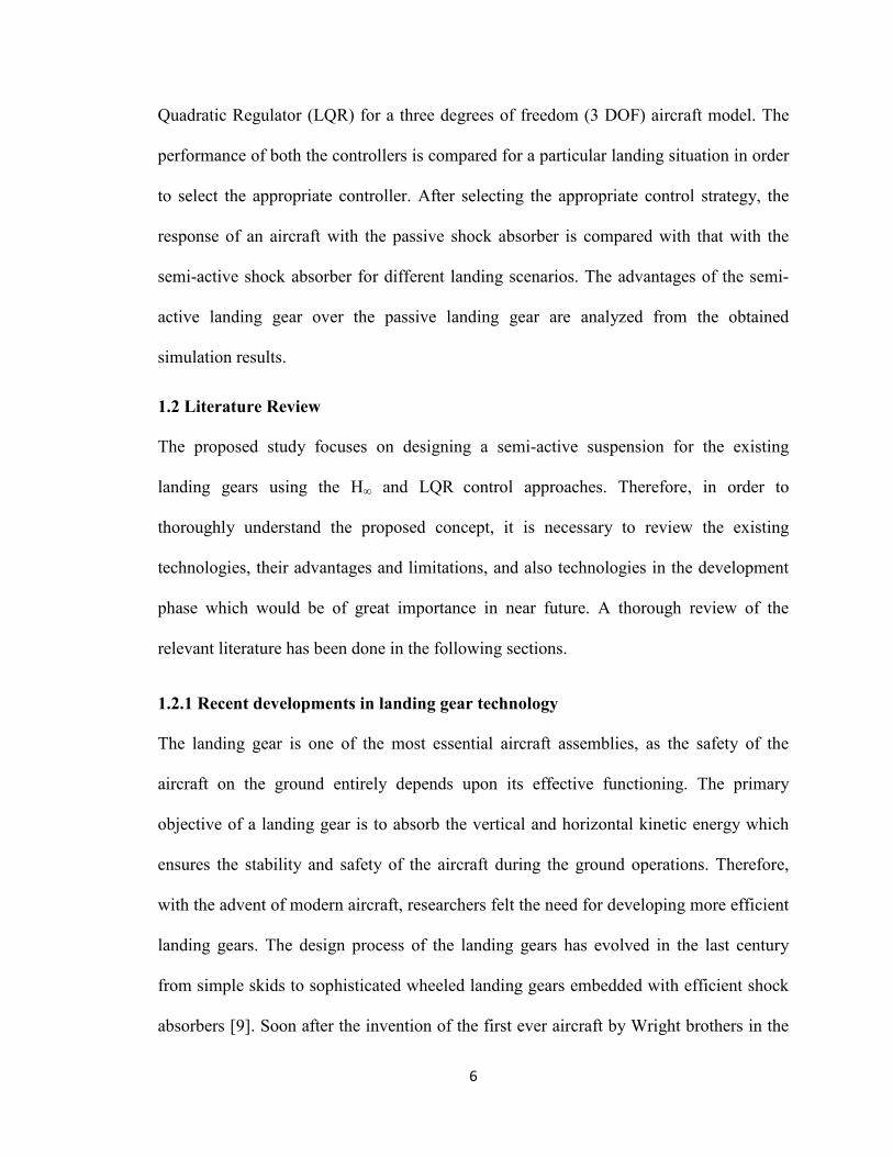
1.2.1.1 Oleo-pneumatic struts: Heart of today’s landing gear technology
The concept of oleo finds its roots back in 1905 when it was first implemented and
patented as a recoil device for large cannons [30]. The struts are called Oleo-pneumatic
because their principle of operation involves using the combination of compressible gas
and incompressible fluid for providing the spring and the damping effects, respectively. It
consists of two cylindrical chambers. The upper chamber is filled with gas charge while
the lower one is filled with the kerosene based mineral oil. Because of the rapid
9
movement of the piston inside the cylinder, large amount of heat is generated which has
to be dissipated effectively. Due to the high heat involved during this process, the gas
charge to be filled in the upper chamber must be an inert gas which would prevent the
explosion of the oil vapour in case of temperature rise beyond a certain level [31].
Therefore, for heavy aircraft it is mandatory for the shock absorber manufacturers to use
the nitrogen or other inert gas as a gas charge.
The gas charge in the upper chamber supports the aircraft weight and the oil
contained in the lower chamber provides the damping effect during the operation. At the
time of touchdown, the strut operates by pushing the chamber of oil against the chamber
of dry air or nitrogen. The dissipation of energy takes place when oil flows through one
or more orifices. A landing aircraft inevitably rebounds after the initial impact. During
this phase, the pressurized air forces the oil back to the lower chamber through the recoil
orifices. The rate of flow of oil through the recoil orifices determines the extent of
rebound. If oil flows too quickly through the orifice, aircraft rebounds upwards rapidly.
On the other hand, if oil flow is too slow, the oscillations will not be damped out
effectively during soft landing and taxiing phases [1], [2].
The spring force in an oleo strut is provided by the compression and expansion of
gas and the damping force by the fluid passing through the orifice. The orifice area
changes as the metering pin moves up and down through the orifice. By appropriately
designing the metering pin, it is possible to achieve the required damping force [30], [31].
However, sometimes because of the conflicting damping requirements, the efficiency of
Oleo dampers is reduced which necessitates the need for developing the controllable
dampers which would be able to provide variable damping forces. Magnetorheological
10
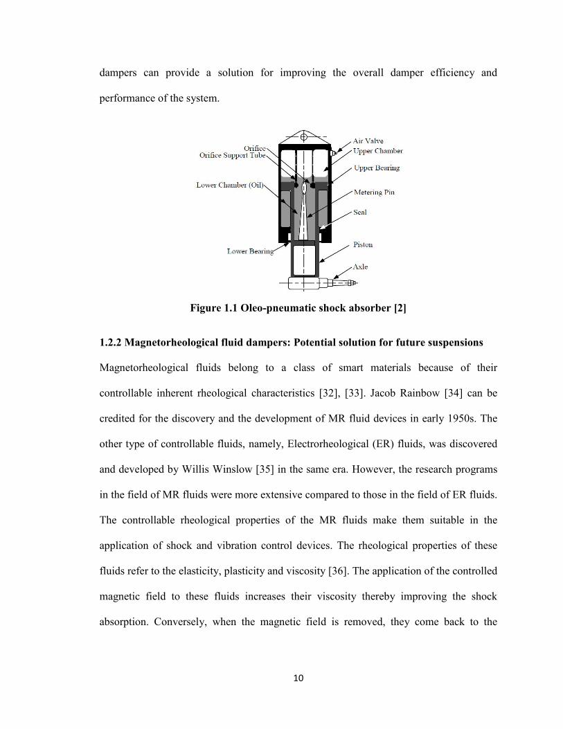
dampers can provide a solution for improving the overall damper efficiency and
performance of the system.
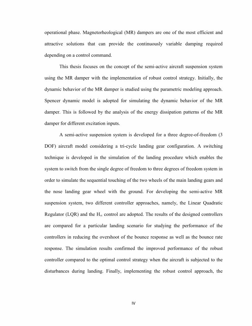
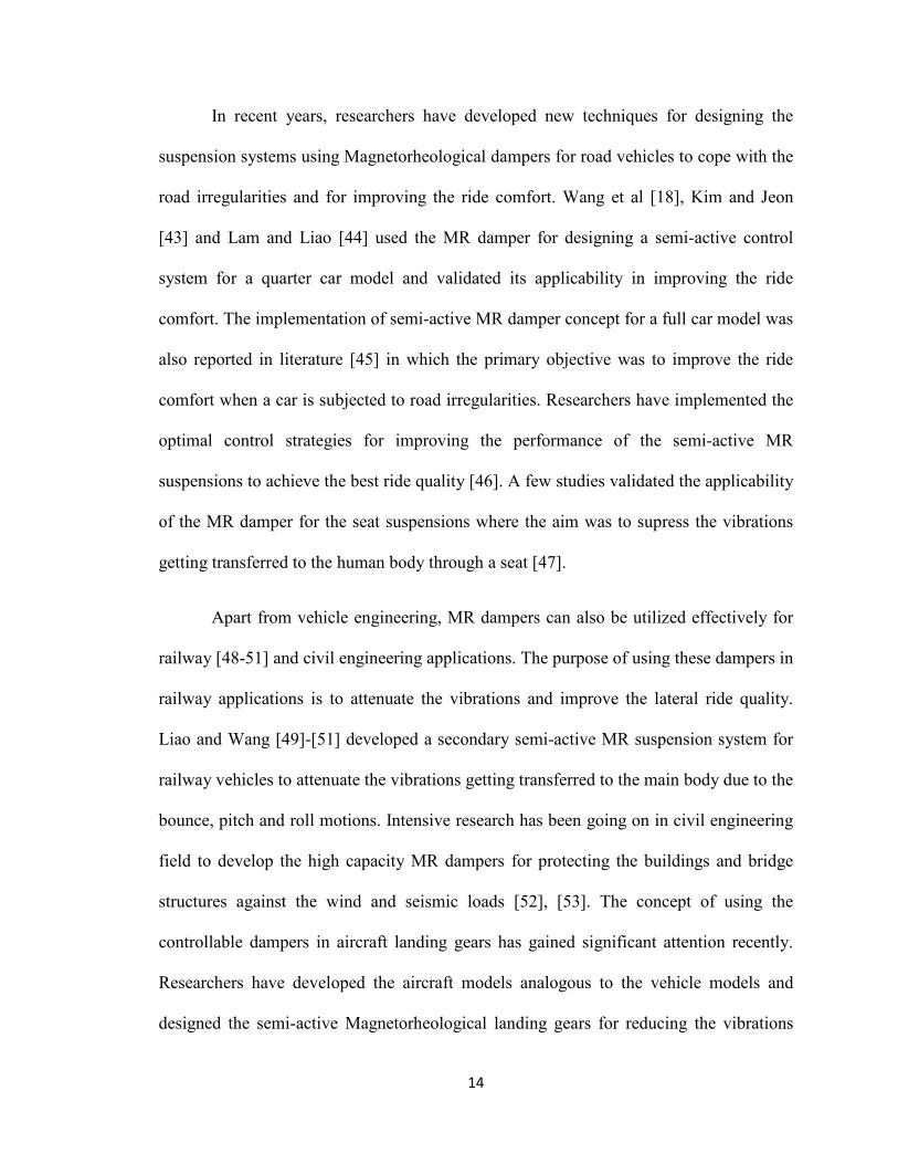
Figure 1.1 Oleo-pneumatic shock absorber [2]
1.2.2 Magnetorheological fluid dampers: Potential solution for future suspensions
Magnetorheological fluids belong to a class of smart materials because of their
controllable inherent rheological characteristics [32], [33]. Jacob Rainbow [34] can be
credited for the discovery and the development of MR fluid devices in early 1950s. The
other type of controllable fluids, namely, Electrorheological (ER) fluids, was discovered
and developed by Willis Winslow [35] in the same era. However, the research programs
in the field of MR fluids were more extensive compared to those in the field of ER fluids.
The controllable rheological properties of the MR fluids make them suitable in the
application of shock and vibration control devices. The rheological properties of these
fluids refer to the elasticity, plasticity and viscosity [36]. The application of the controlled
magnetic field to these fluids increases their viscosity thereby improving the shock
absorption. Conversely, when the magnetic field is removed, they come back to the
11
normal state. This basic property can be utilized in the semi-active vibration control
approaches.
Magnetorheological fluid is basically, a composition made of the magnetizable
particles dispersed randomly in liquid medium, called carrier oil, with a stabilizer [37].
The liquid medium is usually an organic or aqueous solution with insulation properties.
Commonly used liquid media for preparing the MR fluid includes petroleum based oils,
silicon oil, kerosene, mineral oils, synthetic hydrocarbon oils, polyester, polyether, water
etc. The liquid medium used for a particular application must possess good temperature
stability [38], [39]. The particles dispersed in carrier oil are iron based micron-sized
particles having size in the range of 1-10 μm. These particles are magnetically soft which
helps their smooth transition from polarized state to a normal state when the magnetic
field is removed. The most commonly used magnetisable particles are carbonyl iron
powder based, which is a product of decomposition of iron pentacarbonyl. However, the
high density of iron powders (7.8 g/cm3) compared to the carrier liquid poses some
restriction on fluid re-dispersion as the particles settle down at the bottom. Research has
been going on to reduce the size of these particles to a nano-scale in order to facilitate a
smooth re-dispersion of a carrier fluid. The third element which completes the MR fluid
composition is a stabilizer which serves the function of maintaining the agglomerative
stability as well as the sedimental stability which prevent the particles from sticking
together and settling down at the bottom with time. For a fluid immersed with coarse
particles, silica gel is used as a stabilizer whereas the ionic surfactant such as oleic acid is
used for the fluids immersed with finely dispersed particles [36]-[38].
12
Magnetorheological fluids possess a unique property of transforming from a free
flowing state to a highly viscous semi-solid state when exposed to a magnetic field. In a
typical MR damper device, when a current is passed through a coil placed adjacent to the
fluid, the randomly dispersed iron particles in carrier oil acquire the dipole moment in
alignment with the applied magnetic field. This process forms a chain of iron particles
which is perpendicular to the direction of fluid flow thereby restricting it. In other words,
velocity of fluid flow decreases. This effect continues as long as the magnetic field is
maintained. Once the magnetic field is removed, iron particle chains are broken and the
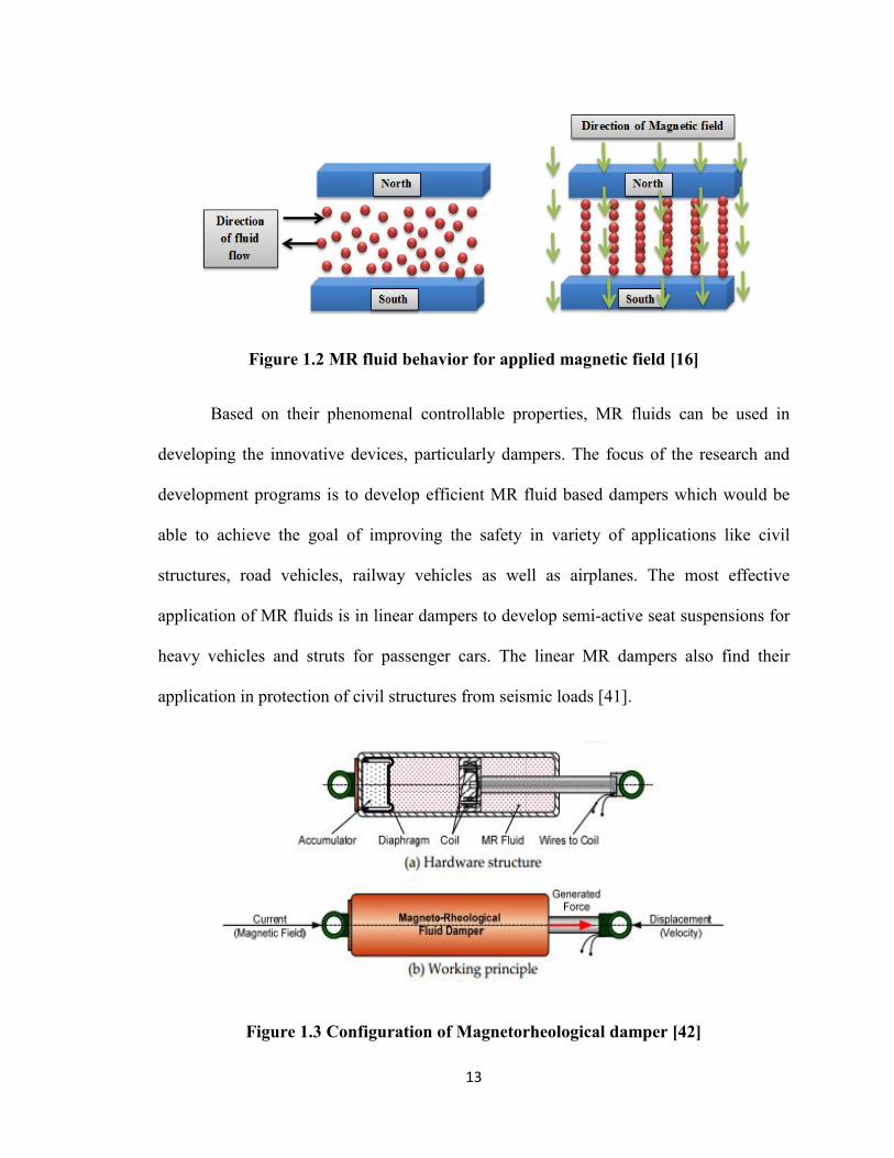
fluid comes back to its normal state. This phenomenon can be visualized from figure 1.2.
This transformation takes place in milliseconds and is reversible, which allows the fluid
to return back to its normal state when magnetic field is removed. This property can be
utilized in MR fluid based devices to achieve variable damping, particularly in the shock
and vibration attenuation applications [21]-[24]. In the absence of magnetic field, these
fluids behave like Newtonian fluids having viscosity ranging from 0.1 to 1 Pa at room
temperature. With the application of magnetic field of 150-200 kA/m, the dynamic yield
strength of 50-100 kpa can be achieved which is significant in the applications where
sudden impacts have to be attenuated quickly. The operating temperature range of these
fluids span from - 40 to 1500 C with minimal variation in yield strength. Generally, these
fluids are not affected by the contaminants during the manufacturing process. Because of
the dispersed iron particles, the density of these fluids ranges from 3-4 g/cm3. The
available devices which work on the MR effect typically requires 2-50 Watt power
source [21]-[24], [38]-[40].
13
Figure 1.2 MR fluid behavior for applied magnetic field [16]
Based on their phenomenal controllable properties, MR fluids can be used in
developing the innovative devices, particularly dampers. The focus of the research and
development programs is to develop efficient MR fluid based dampers which would be
able to achieve the goal of improving the safety in variety of applications like civil
structures, road vehicles, railway vehicles as well as airplanes. The most effective
application of MR fluids is in linear dampers to develop semi-active seat suspensions for
heavy vehicles and struts for passenger cars. The linear MR dampers also find their
application in protection of civil structures from seismic loads [41].
Figure 1.3 Configuration of Magnetorheological damper [42]
14
In recent years, researchers have developed new techniques for designing the
suspension systems using Magnetorheological dampers for road vehicles to cope with the
road irregularities and for improving the ride comfort. Wang et al [18], Kim and Jeon
[43] and Lam and Liao [44] used the MR damper for designing a semi-active control
system for a quarter car model and validated its applicability in improving the ride
comfort. The implementation of semi-active MR damper concept for a full car model was
also reported in literature [45] in which the primary objective was to improve the ride
comfort when a car is subjected to road irregularities. Researchers have implemented the
optimal control strategies for improving the performance of the semi-active MR
suspensions to achieve the best ride quality [46]. A few studies validated the applicability
of the MR damper for the seat suspensions where the aim was to supress the vibrations
getting transferred to the human body through a seat [47].
Apart from vehicle engineering, MR dampers can also be utilized effectively for
railway [48-51] and civil engineering applications. The purpose of using these dampers in
railway applications is to attenuate the vibrations and improve the lateral ride quality.
Liao and Wang [49]-[51] developed a secondary semi-active MR suspension system for
railway vehicles to attenuate the vibrations getting transferred to the main body due to the
bounce, pitch and roll motions. Intensive research has been going on in civil engineering
field to develop the high capacity MR dampers for protecting the buildings and bridge
structures against the wind and seismic loads [52], [53]. The concept of using the
controllable dampers in aircraft landing gears has gained significant attention recently.
Researchers have developed the aircraft models analogous to the vehicle models and
designed the semi-active Magnetorheological landing gears for reducing the vibrations
15
getting transferred to the fuselage during landing and taxiing phases. A 2 DOF aircraft
model representing the aircraft mass and wheel mass is the most commonly used model
for the vibration analysis during landing phase, particularly. Because of the wide range of
applications these dampers offer, they can be considered as the most effective solution for
developing the intelligent damping systems for the future applications.
1.2.3 Semi-active suspension systems
The controllable properties of the Magnetorheological fluids can be used for developing
the semi-active dampers which are capable of providing the variable damping without
compromising efficiency. The intelligent damping concept has been widely used in
vehicles, civil structures, railway vehicles, as well as in aerospace systems. The primary
goal of implementing a semi-active suspension concept in vehicles and aircraft is to
improve the passenger comfort and safety and to increase the stability whereas in the civil
engineering field, this concept has been widely used for the protection of buildings and
bridges against the wind and seismic loads.
The existing passive suspension systems are capable of dissipating energy
effectively at a constant damping rate. Because of the unchangeable damping properties,
variable damping forces cannot be generated which makes them unsuitable for the
applications where the varying damping force is required depending on the operating
conditions. In order to generate a force corresponding to the excitation input, the concept
of the active and the semi-active suspensions was proposed in early 1950s. In active
suspension systems, the force generating device used is the hydraulic actuator which
requires a hydraulic power supply to operate. The actuator replaces the spring-damper
configuration in the conventional passive dampers and generates the force relative to the
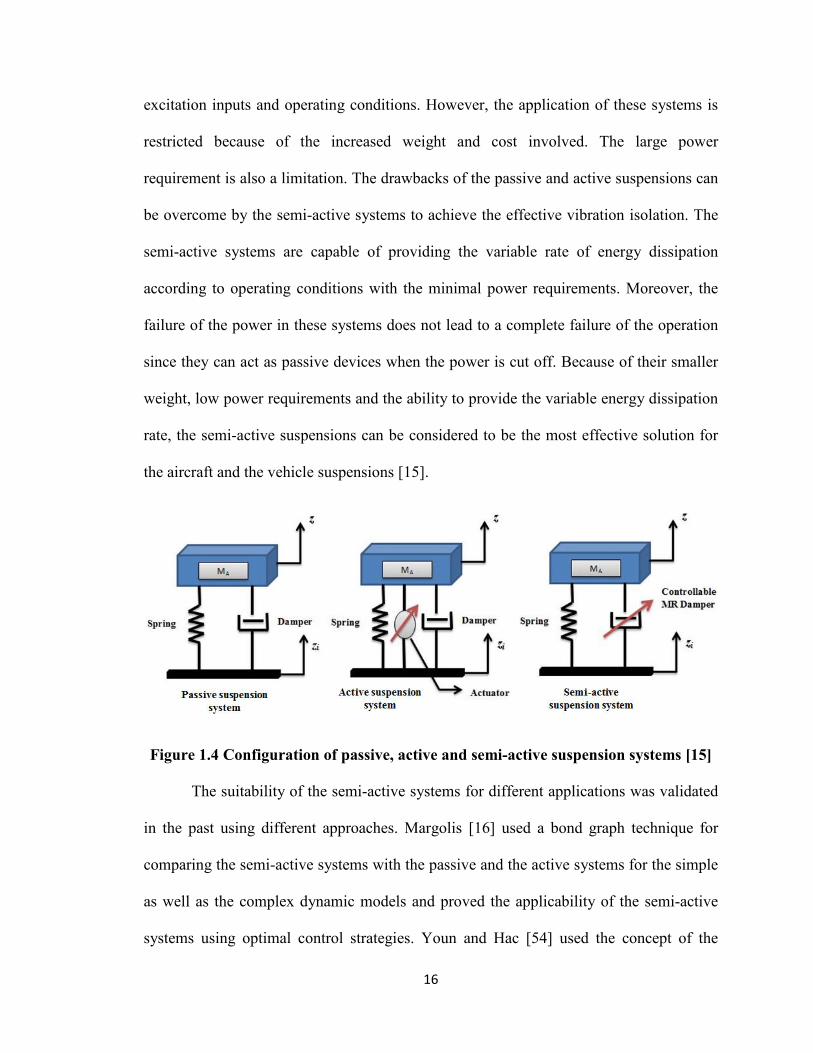
16
excitation inputs and operating conditions. However, the application of these systems is
restricted because of the increased weight and cost involved. The large power
requirement is also a limitation. The drawbacks of the passive and active suspensions can
be overcome by the semi-active systems to achieve the effective vibration isolation. The
semi-active systems are capable of providing the variable rate of energy dissipation
according to operating conditions with the minimal power requirements. Moreover, the
failure of the power in these systems does not lead to a complete failure of the operation
since they can act as passive devices when the power is cut off. Because of their smaller
weight, low power requirements and the ability to provide the variable energy dissipation
rate, the semi-active suspensions can be considered to be the most effective solution for
the aircraft and the vehicle suspensions [15].
Figure 1.4 Configuration of passive, active and semi-active suspension systems [15]
The suitability of the semi-active systems for different applications was validated
in the past using different approaches. Margolis [16] used a bond graph technique for
comparing the semi-active systems with the passive and the active systems for the simple
as well as the complex dynamic models and proved the applicability of the semi-active
systems using optimal control strategies. Youn and Hac [54] used the concept of the
17
semi-active suspension for the 2 DOF vehicle model by implementing the optimal control
strategies for the purpose of improving the ride comfort, road holding and the suspension
rattle speed. Sims and Stanway [55] developed a semi-active suspension system for a
quarter car model to prove the performance gains of the semi-active suspensions over the
passive suspensions. A controllable viscous damper with a force feedback concept was
developed for this study. To improve the performance of the semi-active vehicle
suspensions, researchers have developed the robust control strategies such as H∞ control
in the recent past [17]. The application of the semi-active suspension systems in the
aircraft landing gears is limited. No aircraft has been embedded with the semi-active
struts so far. However, the research growth for developing the concept of the semi-active
landing gears has been prolific [7], [12], [17], [28], [29], [56], [57]. Sivakumar and Haran
[28] developed a semi-active landing gear for the 2 DOF aircraft model using the
Proportional Integral Derivative (PID) controller to improve the ride comfort of the
aircraft subjected to the runway excitations during landing, take-off and taxiing phases.
Zapateiro et al [29] used the adaptive control approach for developing and comparing the
performance of the active and the semi-active landing gears for the purpose of improving
the passenger comfort during the aircraft ride. The concept of the adaptive aircraft shock
absorbers was proposed by Mikulowski and Holnicki-Szulc [56] to cope with the
variations in the landing conditions and to improve the impact absorption capacity.
Kruger [57] designed a semi-active landing gear using three different control approaches
and compared the simulated performance of the passive, active and the semi-active
system for a multibody aircraft model of a transport aircraft. The criterion for comparing
these systems was the vertical acceleration transmitted to the fuselage during landing. Su
18
et al [57] developed a predictive control algorithm for the nonlinear model to design a
semi-active landing gear which could sustain the shocks during the landing and the
taxiing phases and provide the adaptive damping for varying operating conditions. The
reviewed literature is a clear indicator of the applicability of the semi-active systems in
the aircraft landing gears as well as for other applications in near future.
1.2.4 Control strategies for the development of intelligent suspensions
The evolution of the development of the control approaches for building the most
efficient semi-active suspensions for the vehicles [17], [19], [43], [55] and aircraft [12],
[20] [28], [29], [56]-[60] has been remarkable so far. Lin et al [20] proposed a fuzzy PID
controller for the landing gear system in order to reduce the accelerations transmitted to
the fuselage during landing. A hybrid control algorithm combining the advantages of the
PID and fuzzy control was developed and validated through a simulation approach. An
active and a semi-active landing gear concept using a PID controller was used by Wang
et al [27] and Sivakumar and Haran [28], respectively, to reduce the vertical motion of
the aircraft body during landing and other phases. Considering the passenger comfort and
aircraft fatigue life as the validation criterion, the applicability of the active landing gear
concept was proved. Zapateiro et al [29] developed a concept of the adaptive
backstepping control of the landing gear suspension using the robust H∞ control approach
for the purpose of improving the damping performance during different phases of the
aircraft operation.
A few techniques to optimize the controllers for the landing gears were also
reported, previously [56] by selecting the landing gear efficiency as an objective function.
Kruger [57] used three different control approaches namely; a skyhook controller, a fuzzy
19
logic controller and a state feedback controller for developing the semi-active landing
gear for the transport aircraft and designed a multi-objective optimization algorithm to
optimize the control parameters of all the three controllers. A sliding model controller
was utilized by Choi and Werely [59] to design the MR landing gear. Ghiringhelli [60]
proved the applicability of the semi-active landing gears by optimally controlling the
orifice area in the dampers to reduce the vertical impact on the aircraft during landing.
Ghiringhelli and Gauldi [61] developed a multibody aircraft model through ADAMS
simulation and validated the control approach for the landing gear drop test. The
developed model is a good approximation of the real landing scenario. The primary goal
of developing the semi-active landing gears using the optimal controllers is to provide
safety and comfort to the passengers and reduce the fuselage vibrations during landing
and taxiing.
1.3 Problem Definition
The aircraft, during its lifetime, is subjected to varying operating conditions in the air as
well as on the ground. As landing is the most critical phase amongst all the operational
phases, there is a need to design the most efficient landing gears. The shock absorber,
which absorbs huge impact energy during the landing phase, is considered as the heart of
the landing gear assembly and therefore, it becomes necessary to increase its performance
efficiency and the life span. Though the existing shock absorbers are the most efficient
till date, they are not able to meet the variable damping requirements to cope with the
varying operating conditions. The problems such as bad weather conditions, runway
unevenness and pilot inaccuracies might arise during the aircraft operation which could
lead to accidents, sometimes. In such critical scenarios, it is necessary to have the most
20
efficient and the robust damping system which would prevent the aircraft from the
potential accidents. The semi-active suspensions with the robust control strategies could
prove to be a solid solution for preventing the potential aircraft accidents specifically,
during landing.
1.4 Thesis Objectives
The literature review and the problem definition presented in the previous sections
provide a strong basis for defining the objectives of this study. The specific objectives of
this study are as follows:
• Study and analyze the force-velocity characteristics of the Magnetorheological
damper to understand their dynamic behaviour for the sinusoidal excitations.
Spencer model and sigmoid model are selected and a force velocity dynamic
behavior is simulated using MATLAB based on the data available in the previous
literature to validate their applicability.
• Analyze the energy dissipation characteristics of the MR dampers. Derive the
equations for the energy dissipation of the MR damper in one cycle for a
sinusoidal excitation and plot the graphs of the energy dissipated in one cycle
against time. Plot the graphs of dissipated energy against the changing currents
and frequencies.
• Develop a 3 DOF dynamic model of an aircraft embedded with a tricycle landing
gear system and derive the equations of motion. A state-space approach is utilized
for representing the system and developing the controller.
21
• Synthesize two different controllers, namely, a Linear Quadratic Regulator (LQR)
and a robust H∞ controller for developing the semi-active suspension system with
MR damper as an actuator for the selected aircraft model.
• Validate the applicability and robustness of the designed semi-active suspension
system by subjecting the aircraft to different landing scenarios considering
runway roughness.
1.5 Thesis Organization
A thorough review of the relevant literature is presented in chapter 1 for developing a
basic understanding of the concepts that will be implemented in the subsequent chapters.
A problem definition and the thesis objectives are also presented in chapter 1.
Chapter 2 includes the study and analysis of the force-velocity characteristic of the MR
damper in order to understand its dynamic behaviour. Various parametric and non-
parametric models are reported for understanding the dynamic behaviour of the MR
dampers. Finally, the two models, namely, Spencer model and Sigmoid model are
selected and the response of the damper for the sinusoidal excitations is simulated based
on the data already available in the literature.
Chapter 3 explains the basic concepts regarding the energy dissipation by the MR damper
and its linearization. Spencer model which is used in chapter 2 for simulating the force-
velocity characteristics is selected for analyzing the energy dissipation behaviour of the
MR damper in one cycle for a sinusoidal input. The graph of the energy dissipated in one
cycle is plotted against the time for a particular displacement and frequency input. As
Spencer model is a current dependent model, the relationship of the dissipated energy
22
with increasing currents with a fixed value of the frequency and the displacement input is
depicted graphically. Similarly, the relationship of the dissipated energy with changing
frequencies is plotted for fixed current values.
In chapter 4, a 3 DOF dynamic model of an aircraft is developed and the equations of
motion are derived. A state-space approach is followed for representing the system in
order to synthesize two controllers for the developed system. The aircraft parameters are
selected from the available literature.
Chapter 5 involves the simulation of the actual landing scenario for different sink
velocities. The performance of the two controllers is compared for the purpose of
selecting the appropriate control law. Finally, the response of an aircraft embedded with
the developed semi-active system is plotted and compared with existing passive system.
The applicability and the robustness of the controller are validated by subjecting the
aircraft to the rough landing scenarios.
The important conclusions and the future recommendations are presented in chapter 6.
23
CHAPTER 2
DYNAMIC MODELING OF THE HYSTERETIC
CHRACTERISTICS OF A MR FLUID DAMPER
2.1 Introduction
The Magnetorheological dampers are currently the focus of researchers and engineers
[12] because of their potential to be used for the various engineering applications such as
vehicle suspensions, aircraft landing gears, railway suspensions. A few civil engineering
as well as biomechanical engineering [62], [63] applications have also been reported. The
primary reason for the wide range of applications of the MR dampers is their controllable
viscosity. The current levels required for achieving the required viscosity are also
nominal. These dampers exhibit unique characteristics which enable their rapid transition
from a low viscosity state to a high viscosity state according to the current variations.
Their ability to provide a rapid interface between the mechanical systems and the
electronic controls can be utilized for developing the semi-active systems [21].
In order to build the efficient MR fluid based dampers, it is imperative to
understand their basic principle of operation. Moreover, these dampers exhibit a highly
non-linear hysteretic behaviour which makes the process of the controller design critical.
Therefore, it is necessary to understand the inherent hysteretic nature of these dampers to
address the issue of the controller design. Various dynamic models have been proposed
by the researchers, in the past, for accurately characterizing the behaviour of the MR
dampers. In this section, the basic principle of the MR damper is presented first, followed
by a critical review of the available dynamic models for characterizing the force-velocity
24
(f-v) hysteretic behaviour of these dampers. A simulation approach is adopted by taking
into consideration two different dynamic models to plot and analyze the hysteretic
behaviour of these dampers for a selected range of the sinusoidal excitations. As the data
is taken from the previously available literature, the models are validated by comparing
the simulation results of the f-v characteristics with the results available in the literature.
2.1.1 Operational features of the MR fluid based devices
The Magnetorheological fluid based devices are magnetic field dependent and are
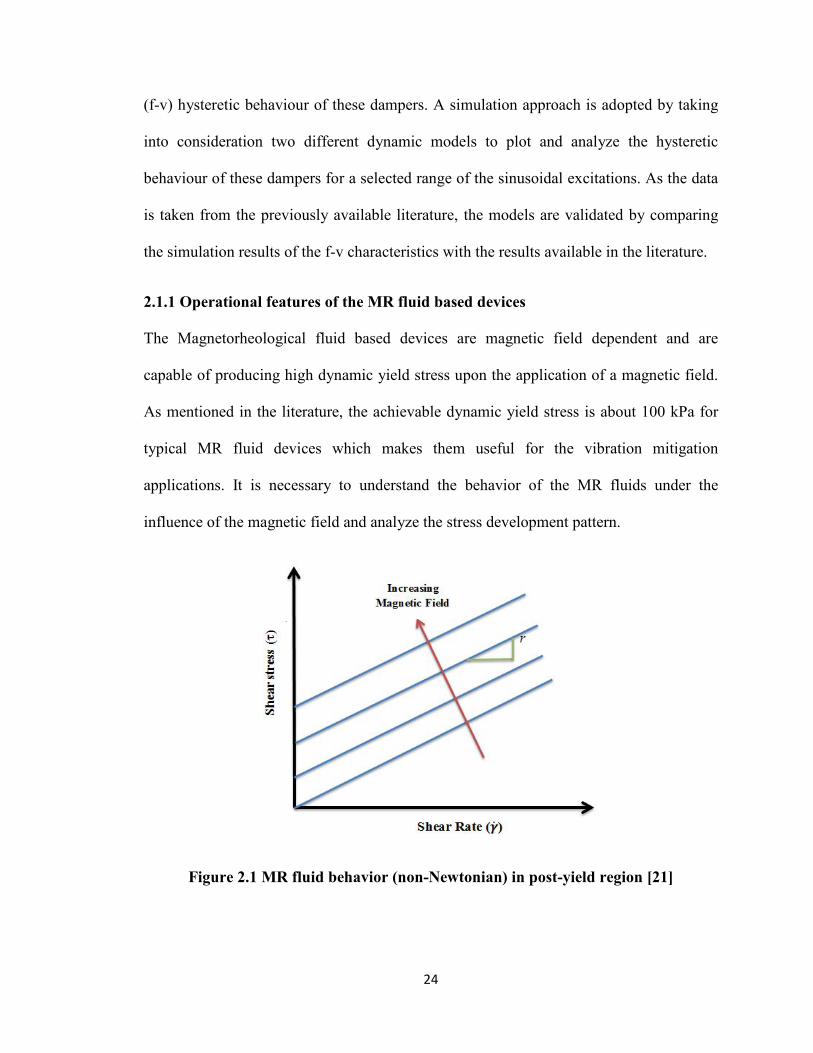
capable of producing high dynamic yield stress upon the application of a magnetic field.
As mentioned in the literature, the achievable dynamic yield stress is about 100 kPa for
typical MR fluid devices which makes them useful for the vibration mitigation
applications. It is necessary to understand the behavior of the MR fluids under the
influence of the magnetic field and analyze the stress development pattern.
Figure 2.1 MR fluid behavior (non-Newtonian) in post-yield region [21]
25
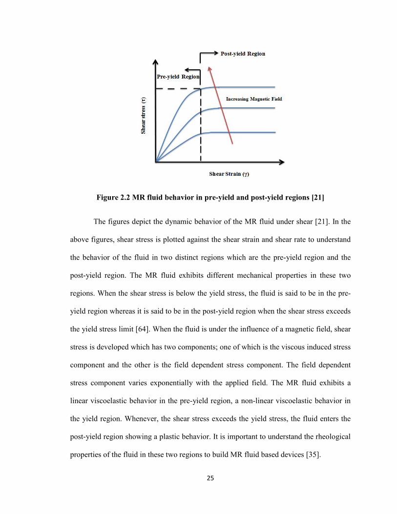
Figure 2.2 MR fluid behavior in pre-yield and post-yield regions [21]
The figures depict the dynamic behavior of the MR fluid under shear [21]. In the
above figures, shear stress is plotted against the shear strain and shear rate to understand
the behavior of the fluid in two distinct regions which are the pre-yield region and the
post-yield region. The MR fluid exhibits different mechanical properties in these two
regions. When the shear stress is below the yield stress, the fluid is said to be in the pre-
yield region whereas it is said to be in the post-yield region when the shear stress exceeds
the yield stress limit [64]. When the fluid is under the influence of a magnetic field, shear
stress is developed which has two components; one of which is the viscous induced stress
component and the other is the field dependent stress component. The field dependent
stress component varies exponentially with the applied field. The MR fluid exhibits a
linear viscoelastic behavior in the pre-yield region, a non-linear viscoelastic behavior in
the yield region. Whenever, the shear stress exceeds the yield stress, the fluid enters the
post-yield region showing a plastic behavior. It is important to understand the rheological
properties of the fluid in these two regions to build MR fluid based devices [35].
26
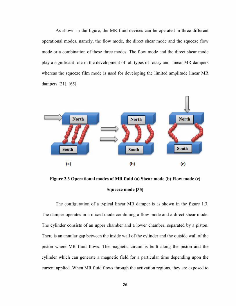
As shown in the figure, the MR fluid devices can be operated in three different
operational modes, namely, the flow mode, the direct shear mode and the squeeze flow
mode or a combination of these three modes. The flow mode and the direct shear mode
play a significant role in the development of all types of rotary and linear MR dampers
whereas the squeeze film mode is used for developing the limited amplitude linear MR
dampers [21], [65].
Figure 2.3 Operational modes of MR fluid (a) Shear mode (b) Flow mode (c)
Squeeze mode [35]
The configuration of a typical linear MR damper is as shown in the figure 1.3.
The damper operates in a mixed mode combining a flow mode and a direct shear mode.
The cylinder consists of an upper chamber and a lower chamber, separated by a piston.
There is an annular gap between the inside wall of the cylinder and the outside wall of the
piston where MR fluid flows. The magnetic circuit is built along the piston and the
cylinder which can generate a magnetic field for a particular time depending upon the
current applied. When MR fluid flows through the activation regions, they are exposed to
27
the magnetic field to achieve the desirable viscous force. This way, by controlling the
level of current at specific times, it is possible to magnetize the fluid and obtain high
dynamic yield stresses according to the application requirements [66]. For the aircraft
applications, these devices can prove their potential in mitigating the excessive vibrations
at the time of landing, by generating the required viscous forces for nominal current
levels.
2.2 Review of MR Damper Models
The non-linear hysteretic characteristics of the MR dampers refer to the force-velocity
and force-displacement relations. The MR dampers exhibit inherent hysteretic behavior
which has to be predicted accurately by using different modeling techniques in order to
effectively implement these dampers for the variable damping applications. The force-
velocity characteristic is a plot of variation of a damping force with the piston velocity
which can be described in two distinct regions called the post-yield region and the pre-
yield region. The shape of the hysteresis loop varies according to the variations in the
parameters such as frequency, amplitude and current of the applied excitation signals.
Many models have been developed so far, for accurately predicting the dynamic
hysteretic behavior of the MR dampers for the purpose of developing effective control
strategies [21]. The developed models must be applicable for a wide range of excitation
conditions and should satisfy the validity criteria such as robustness, simplicity, accuracy
and reversibility. Based on their properties, the MR damper models can be classified into
two main categories; the dynamic models and the quasi-static models. The quasi-static
models prove their ability in designing the MR damper but are not able to predict the
non-linear hysteresis characteristics. The drawbacks of the quasi-static models can be
28
overcome by the dynamic models which can predict the non-linear hysteresis, making the
process of the controller design less complicated.
The dynamic models can be further classified as the parametric dynamic models
and the non-parametric dynamic models. The non-parametric modeling methods make
use of the analytical approach for characterizing the behavior of the MR dampers. These
models are applicable for the linear as well as non-linear systems because of their
robustness [21]. Choi et al [67] proposed a polynomial model, which is a non-parametric
model, to predict the MR damper hysteretic characteristics. In this model, the MR damper
force is represented as a polynomial function in terms of piston velocity. However, the
order of the polynomial was found out by trial and error method for accurately capturing
the force-velocity hysteresis. Jin et al [68] proposed a black-box modeling technique for
the MR dampers to cope with the structural control problems. The comparison between
the non-linear black-box modeling and the semi-physical modeling is also reported in the
literature [69]. The neural network model suggested by Wang and Liao [70] can be used
for modeling and controlling the MR damper behavior as it is evident from the literature
that the feed-forward neural networks can find an approximate solution for any
continuous function. The other non-parametric models involve the fuzzy model, the
Ridgnet model, the wavelet model and the multi-function model [21].
The parametric dynamic models represent the other class of the dynamic models.
The parametric models represent a system as a collection of elements such as the springs
and dampers and require a parameter identification procedure for modeling the dynamic
behavior of the MR dampers. The complexity of the model can be judged depending
upon the number of parameters to be identified. The parametric dynamic models fall into
29
various classes, namely, the Bouc-Wen hysteresis operator based dynamic models, the
biviscous models, the sigmoid function based models, the Bingham model-based
dynamic models, the viscoelastic plastic models, the hyperbolic tangent function models,
the equivalent models and few others [21]. Werely et al [71] implemented four different
parametric models for predicting the force-velocity hysteresis and the energy dissipation
analysis of the MR dampers. These models involve the linearized equivalent viscous
damping model, the non-linear Bingham plastic model, the non-linear biviscous model
and the non-linear biviscous hysteretic model. The proposed Bingham plastic model
assumes the material to be rigid in the pre-yield zone which starts flowing like a
Newtonian fluid once the damper force exceeds the yield force. In the non-linear
biviscous model proposed by Stanway [72], the material is assumed to be plastic in both
pre-yield and the post-yield regions and the damping in the pre-yield condition is
assumed to be significantly higher than that in the post-yield condition. The extension of
the non-linear biviscous model is the non-linear biviscous hysteretic model, which is a
four parameter model for accurately describing the hysteresis phenomenon in the pre-
yield region. The sigmoid function based models [73]-[75] use the symmetric and
asymmetric sigmoid functions for depicting the force-velocity relation. The Bouc-Wen
hysteresis operator based dynamic models are the most widely used models for accurately
identifying the hysteretic characteristics for control purpose. Spencer [76] proposed a
novel model based on the Bouc-Wen hysteresis model which could accurately predict the
inherent non-linear behavior of the MR dampers. The accuracy of the model was
validated for a wide range of operating conditions. Further modifications in the Bouc-
Wen model were suggested and implemented by Dominguez et al [77], [78] for
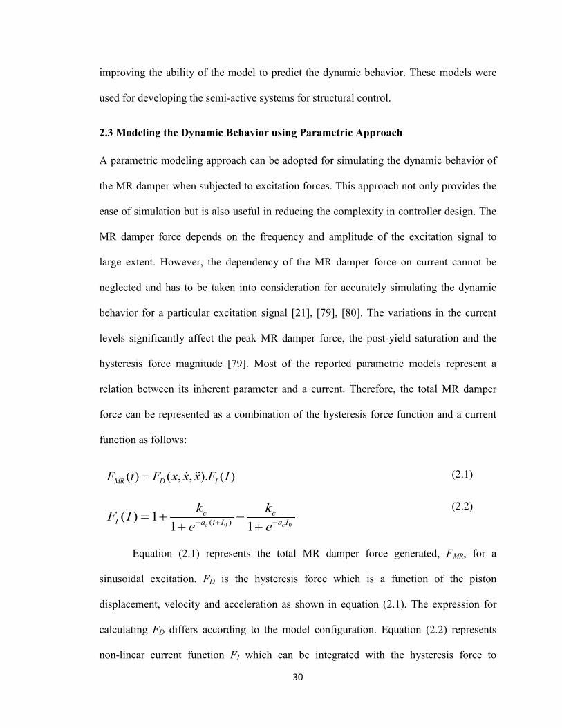
30
improving the ability of the model to predict the dynamic behavior. These models were
used for developing the semi-active systems for structural control.
2.3 Modeling the Dynamic Behavior using Parametric Approach
A parametric modeling approach can be adopted for simulating the dynamic behavior of
the MR damper when subjected to excitation forces. This approach not only provides the
ease of simulation but is also useful in reducing the complexity in controller design. The
MR damper force depends on the frequency and amplitude of the excitation signal to
large extent. However, the dependency of the MR damper force on current cannot be
neglected and has to be taken into consideration for accurately simulating the dynamic
behavior for a particular excitation signal [21], [79], [80]. The variations in the current
levels significantly affect the peak MR damper force, the post-yield saturation and the
hysteresis force magnitude [79]. Most of the reported parametric models represent a
relation between its inherent parameter and a current. Therefore, the total MR damper
force can be represented as a combination of the hysteresis force function and a current
function as follows:
(2.1)
(2.2)
Equation (2.1) represents the total MR damper force generated, FMR, for a
sinusoidal excitation. FD is the hysteresis force which is a function of the piston
displacement, velocity and acceleration as shown in equation (2.1). The expression for
calculating FD differs according to the model configuration. Equation (2.2) represents
non-linear current function FI which can be integrated with the hysteresis force to
( ) ( , , ). ( )MR D IF t F x x x F I=
0 0( )( ) 11 1c c
c cI a i I a I
k kF Ie e− + −= + −
+ +
31
calculate the total MR damper force, FMR. Although, the method for calculating the
hysteresis force differs for each model, the expression for the current function FI, to be
integrated, remains the same. Therefore, in order to understand the effects of applied
current on the MR damper force, Spencer model and Sigmoid model are selected for
simulating the force-velocity hysteretic behavior of the MR damper. The parameters of
Spencer and Sigmoid model presented in [79] and [80] are selected for analyzing the
hysteretic behavior. The simulation results are compared and validated with the results in
[79]. In the following sections, the equations for Spencer model and Sigmoid model are
expressed to predict the dynamic behavior of the MR dampers analytically. A simulation
approach is adopted and the force-velocity behavior is plotted in MATLAB/SIMULINK
for both the models.
2.3.1 Spencer model
Spencer model is an extension of the Bouc-Wen model with the addition of the spring
and damper elements for improving the smoothness of the hysteretic characteristics. The
dynamic equations of Spencer model for the damper force calculations can be derived
from the model configuration as shown in figure 2.4. [76], [79], [81].
Figure 2.4 Spencer (extended Bouc-Wen) model for MR dampers [76]
32
The total MR damper force generated by the system is
0 0( ) ( ) ( )iD rF p c z q k z q k z zα= + − + − + −
(2.3)
where, kr is the MR damper accumulator stiffness and zi is the initial displacement
associated with spring kr and the control stiffness at larger velocities is represented by k0.
The relative displacement between the ends of the MR damper is given by z and q
represents the internal state to account for the roll-off effect caused by the damping
coefficient cr. The restoring force FD involves the non-dimensional auxiliary variable p
which represents the hysteresis of the MR damper model.
(2.4)
where, β and γ are the non-dimensional values to describe the hysteretic loop in the
negative and positive slopes. Also, a is a non-dimensional value for defining the loop size
with respect to the relative velocity of the two ends of MR damper. The transition of the
MR fluid from elastic to plastic state should be smooth to eliminate the subjective feel of a
damper. The smoothness of the transition between the two states is governed by a scalar n.
The equation for q is presented as follows,
(2.5)
The parameter related to the MR fluid yield stress is designated by α. The viscous
damping coefficient at larger velocities is represented by c0. The dashpot represented by cr
is included in the model to account for the roll-off effect, which is observed at low
11( ) ( )n np p p z q z q p A z qγ β−= − − − − + −
( )0 00
( )1
rq p c k z qz
c cα= + + −
+
33
velocities. In order to consider the effect of the magnetic field on the model parameters,
Spencer [76] suggested a linear relationship between the applied voltage and the
parameters α, c0 and cr. However, for the simulation purpose, the methodology suggested
by Wang [15] and Ma [79], [80] is adopted in order to improve the model prediction
abilities. Therefore, a modification in Spencer model can be done by considering the
parameters α, c0 and cr as constants and integrating the non-linear current function shown
in equation (2.2) with the hysteretic force function for predicting the hysteretic behavior
accurately [15], [21], [79], [80].
(2.6)
For the ease of simulation, a hysteretic force function, FD, described in equation (2.3) is
calculated separately and integrated with the non-linear current function. Equation (2.6)
represents the total MR damper force for this model.
2.3.2 Sigmoid model
Sigmoid model is a parametric dynamic model which formulates the hysteretic force
function using the symmetric sigmoid function. This function does not take into account
the current dependency. To consider the effect of current on the MR damper hysteresis
loop, a non-linear current function described in equation (2.2) can be integrated with the
hysteretic force function. The hysteretic force function depends on the displacement,
velocity and the acceleration of the input applied. This function can be described by the
following equation [15], [21], [79], [80].
( )0 0
0 0 ( )( ) ( ) ( ) 11 1c c
ic c
MR r a i I a Ip c z q k z q k z zk k
Fe e
α− + −
+ − + − + −
= ⋅ + − + +
34
(2.7)
In equation (2.7), the term FT represent the transition force. The transition force represents
the value of the force at a particular point at which the hysteresis loop enters the post-yield
region. The governing equation for the transition force can be described as follows,
(2.8)
Another term that is involved in the hysteretic force function equation is the zero force-
velocity intercept, vh. The shape of the hysteresis loop, especially its width varies
according to the variations in vh. The mathematical equation for calculating this term can
be represented as shown below.
(2.9)
It can be interpreted from the above equation that the input excitation conditions have a
significant effect on vh. On the other hand, the dependency of vh on applied current is
nominal. This indicates that for Sigmoid model, the current variations only have a slight
effect on the width of the hysteresis loop.
In equation (2.7), kp and µ are the linear rise coefficient and the hysteresis slope
coefficient which can be formulated as,
(2.10)
( )
( )
1 (1 )1
h
h
x v
D T px veF F k xe
µ
µ
− +
− +
−= +
+
10 (1 )mb v
TF F e= +
0 0( )( ) 11 1
b bh a m i i i
k kv sign x k ve eψ ψ− + −
= + − + +
1 ma vp mk k e−=
35
(2.11)
From the equations presented above, it can be observed that the terms defined above
depend on the term designated as vm which is the peak velocity. In actual practice, the
values of vm cannot be measured directly. However, it is necessary to measure this velocity
in order to depict the force-velocity relationship accurately. The peak velocity vm can be
measured from the instantaneous displacement, velocity ad the acceleration of the applied
input. The equation for measuring the peak velocity vm can be represented as follows.
(2.12)
Therefore, the total MR damper force including the non-linear current function can be
represented as shown in equation (2.13). The constants defined in the above equations are
F0, i0, a0, a1, b1, k0, ka, kb, km and Ψ.
(2.13)
To simulate the response of the MR damper using the above equations it is necessary to
identify the constant parameters involved in these equations. Wang [15] and Ma [79], [80]
presented a methodology for the parameter identification. The parameters identified in
[79] can be used for the simulation in order to validate the developed model.
0
01 m
ak v
µ =+
2( ) ( )mv x xx= −
0 0
( )
( ) ( )
1 (1 ) 11 1 1
h
h c c
x vc c
MR T px v a i I a I
k keF F k xe e e
µ
µ
− +
− + − + −
− = + ⋅ + − + + +
36
2.4 Simulation Results
Based on the hysteretic force equations and the current relationships, a hysteretic force-
velocity behavior is plotted using Spencer model and Sigmoid model described in the
sections (2.3.1) and (2.3.2).
In order to validate the accuracy of the developed Simulink model, the obtained
force-velocity hysteresis curves are compared with the results in [79]. The accuracy of
the Simulink model is necessary to validate since the built Simulink model will be used
again for defining the actuation system for the semi-active aircraft landing gear which is
the main objective of the study. According to the experimental analysis done in [15],
[79], [80] the MR damper is excited by a sinusoidal signal with the amplitude of 6.25
mm. Three different frequency values are selected which are 1.5 Hz, 2.5 Hz and 5Hz. The
applied current values are 0.00 A, 0.25 A, 0.50 A, 0.75 A, 1.00 A, 1.25 A and 1.50 A.
Maintaining the amplitude constant, the hysteretic behavior of the MR damper for a
particular frequency is depicted for seven different current levels. The simulation results
for the hysteretic f-v characteristics for Spencer model and Sigmoid model can be
observed from the following figures.
Figures (2.5)-(2.7) show the results of the force-velocity hysteresis for Spencer
model whereas figures (2.8)-(2.10) depict the behavior for Sigmoid model.
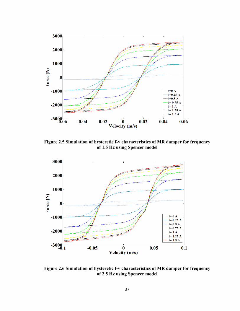
37
Figure 2.5 Simulation of hysteretic f-v characteristics of MR damper for frequency of 1.5 Hz using Spencer model
Figure 2.6 Simulation of hysteretic f-v characteristics of MR damper for frequency of 2.5 Hz using Spencer model
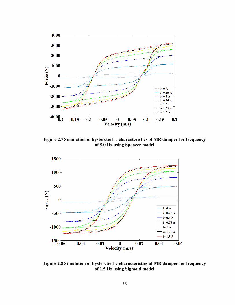
38
Figure 2.7 Simulation of hysteretic f-v characteristics of MR damper for frequency of 5.0 Hz using Spencer model
Figure 2.8 Simulation of hysteretic f-v characteristics of MR damper for frequency of 1.5 Hz using Sigmoid model
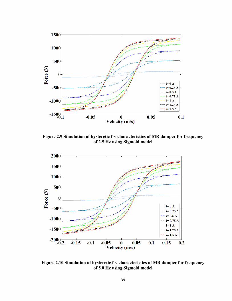
39
Figure 2.9 Simulation of hysteretic f-v characteristics of MR damper for frequency of 2.5 Hz using Sigmoid model
Figure 2.10 Simulation of hysteretic f-v characteristics of MR damper for frequency of 5.0 Hz using Sigmoid model
40
2.5 Discussions
The dynamic behavior of the MR damper can be analyzed from the simulation results of
the hysteretic force-velocity characteristics. The important observations from the
obtained results are summarized as follows:
• For both models, the MR damper behaves as a linear viscous damper when there
is no current applied in a circuit. The force varies approximately linearly with the
velocity, which is depicted as the light grey curve in the figures. It can be
interpreted that the MR damper behaves as a passive device whenever there is no
current in the circuit.
• For small increments in current levels, the magnitude of the MR damper force
increases significantly. The path of the hysteresis loop follows a counter-
clockwise direction when plotted against time. Motion to the right corresponds to
positive acceleration and vice versa. The mean curve of the hysteresis loop
approximately corresponds to the viscous damping coefficient of the MR fluid. In
the pre-yield region, a strong hysteresis can be observed. The force velocity
relationship is linear for larger positive velocities in the post-yield region.
• The variations in the frequency values of the applied signal have a significant
effect on the magnitude of the force as well as on the hysteresis loop. The force
increases with the frequency. Moreover, at higher frequencies, the width of the
hysteresis loop increases in size, especially in case of Spencer model.
• The upper curve in the hysteresis loop depicts the relationship of the MR damper
force with the decreasing velocities whereas the lower curve represents the force
with the increasing velocities. The force velocity relationship is linear for the
41
larger positive velocities. However, when the velocity decreases and before the
loop enters the negative region, the force velocity relation drops off suddenly but
smoothly. This rapid drop is due to bleed or blow-by of fluid between the piston
and the cylinder. This non-linear effect is called the roll-off effect and it allows a
smooth transition between the two operating regions of the MR dampers thereby
avoiding a sudden shock like feeling. A simulation approach using Spencer model
can satisfactorily consider this effect thereby proving its advantages over sigmoid
as well as the other existing models, particularly for the suspension applications.
2.6 Summary
In this chapter, the literature regarding the basic principle of operation of the
Magnetorheological dampers, their characteristics and the dynamic modeling strategies
for describing those characteristics is thoroughly reviewed. A simulation approach was
adopted in order to gain in-depth understanding of the force-velocity hysteretic
characteristics of the Magnetorheological damper using two parametric dynamic models,
namely, Spencer model and Sigmoid model. Both the models were built using
MATLAB/SIMULINK. To validate the accuracy of the models, the results of the
hysteretic force-velocity characteristics are plotted and checked with the results in the
literature. Once the simulation results matched with the results in the available literature,
the two models were compared in order to select the best out of two for further
applications in the remaining part of the study. From the observations, it can be
interpreted that the Spencer model is easy to build and is robust and accurate. Moreover,
it also takes into consideration the roll-off in the lower velocity region of the hysteresis
loop which plays a significant role in building MR damper actuating systems for the
42
semi-active suspensions. Therefore, Spencer model is used for the further analysis in the
next chapter for studying the phenomenon of the energy dissipation by the MR damper
through the simulation approach.
43
CHAPTER 3
ANALYSIS OF THE ENERGY DISSIPATION BY THE
MAGNETORHOLOGICAL DAMPER
3.1 Introduction
A thorough review of the literature suggests that the Magnetorheological dampers are
capable of effectively controlling the vibration. They have a wide range of applications
almost in every stream of engineering. However, achieving the effective vibration
attenuation using the controllable MR dampers is a critical task because of their inherent
non-linearity. The MR dampers exhibit a highly non-linear hysteretic behavior upon the
application of the external signal which is evident from the force-velocity hysteresis
results obtained through simulation in chapter 2. As mentioned in the literature, this
inherent non-linearity poses some limitations in the controller design thereby making the
task of semi-active suspension design more critical.
Since the primary objective of this study is to build an effective semi-active
suspension system for the aircraft landing gears for vibration suppression during landing,
it is necessary to understand completely, the non-linear characteristics of the MR
dampers to facilitate the task of controller design. The force-velocity hysteretic
characteristic gives an understanding of the dynamic behavior of the MR damper to some
extent. However, it is also necessary to analyze the pattern of the energy dissipation by
the MR damper over a cycle. The analysis of the energy dissipation can provide better
understanding of the damping characteristics and also can facilitate the process of
linearizing the MR damper for finding the equivalent viscous damping coefficient for the
given operating conditions to simplify the non-linearity problem.
44
In this chapter, an analysis of the energy dissipation behavior of the MR damper
is carried out. Again, Spencer model, which was used in the previous chapter, is used for
depicting the force-displacement characteristics of the MR damper which are useful for
calculating the energy dissipation by the damper over one cycle. The excitation
conditions are same as those in chapter 2. The energy dissipation behaviour is analyzed
for three different frequencies and seven different current levels. An equivalent viscous
damping coefficient is calculated for each operating condition in order to linearize the
MR damper. Finally, the graphs of the energy dissipated versus the current and the
frequency are plotted. Similarly, the graphs can be plotted for the calculated equivalent
viscous damping coefficients.
3.2 Linearization of the Magnetorheological Damper
The Magnetorheological damper can be linearized using the concept of equivalent
viscous damping [71]. In normal practice, the equivalent damping coefficient (Ceq) is
calculated for approximating the performance of the non-linear MR damper by a
conventional viscous damper. The equivalent viscous damping coefficient provides the
same damping effect as that of the MR damper [82]-[85]. Linearization would facilitate
the understanding of the damping characteristics of the MR dampers.
In order to calculate the equivalent viscous damping coefficient, Ceq, it is
necessary to calculate the amount of energy dissipated by the MR damper in one cycle
for a given input signal. Moreover, since the dynamic behaviour of the MR damper is
analyzed using the current dependent Spencer model, the effect of the current on the
dissipated energy has to be taken into consideration. The rate of energy dissipation is the
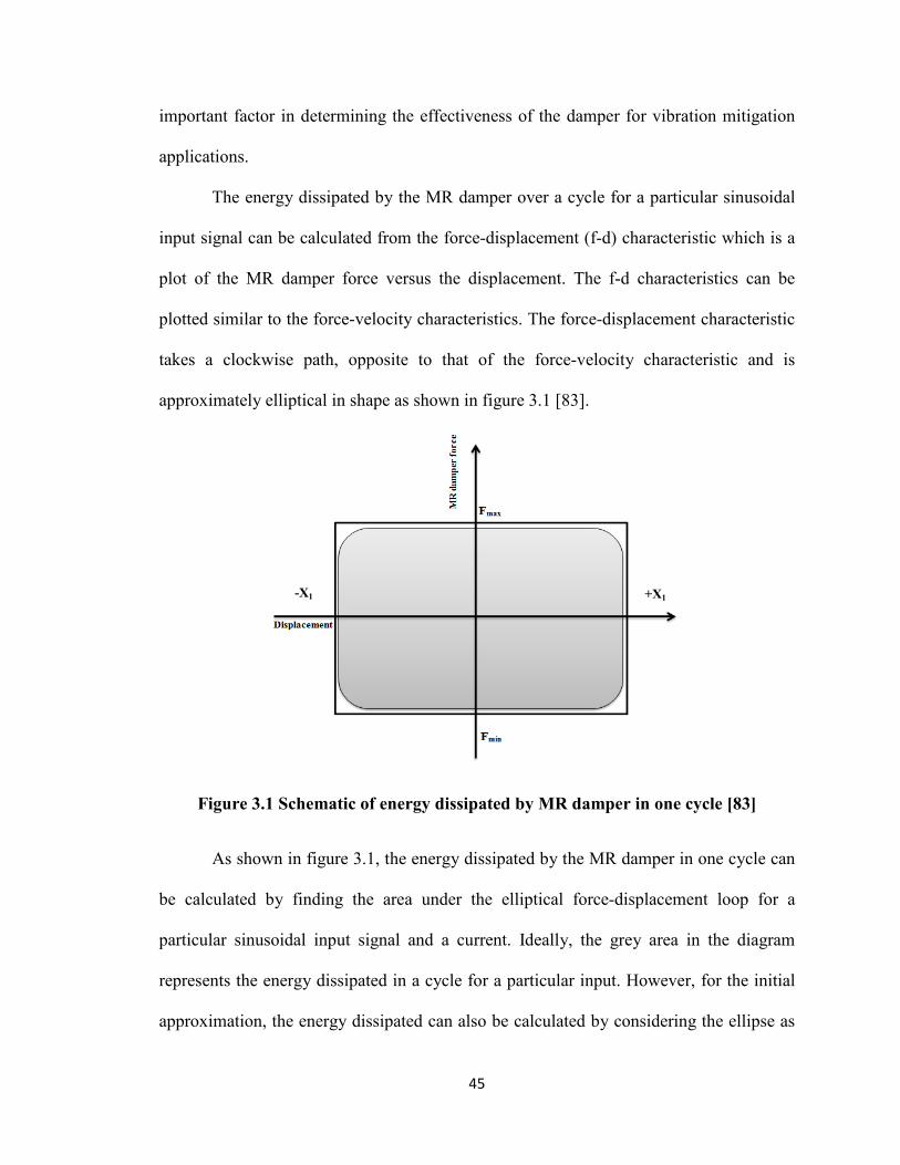
45
important factor in determining the effectiveness of the damper for vibration mitigation
applications.
The energy dissipated by the MR damper over a cycle for a particular sinusoidal
input signal can be calculated from the force-displacement (f-d) characteristic which is a
plot of the MR damper force versus the displacement. The f-d characteristics can be
plotted similar to the force-velocity characteristics. The force-displacement characteristic
takes a clockwise path, opposite to that of the force-velocity characteristic and is
approximately elliptical in shape as shown in figure 3.1 [83].
Figure 3.1 Schematic of energy dissipated by MR damper in one cycle [83]
As shown in figure 3.1, the energy dissipated by the MR damper in one cycle can
be calculated by finding the area under the elliptical force-displacement loop for a
particular sinusoidal input signal and a current. Ideally, the grey area in the diagram
represents the energy dissipated in a cycle for a particular input. However, for the initial
approximation, the energy dissipated can also be calculated by considering the ellipse as
-X1 +X1
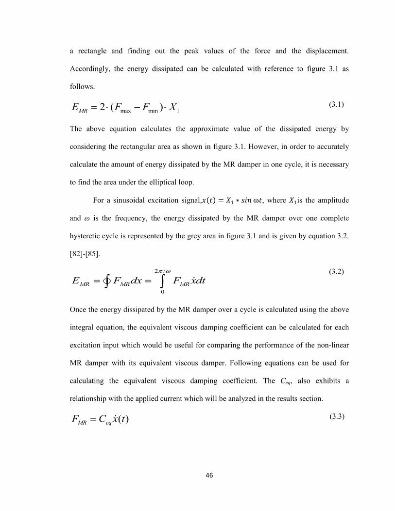
46
a rectangle and finding out the peak values of the force and the displacement.
Accordingly, the energy dissipated can be calculated with reference to figure 3.1 as
follows.
(3.1)
The above equation calculates the approximate value of the dissipated energy by
considering the rectangular area as shown in figure 3.1. However, in order to accurately
calculate the amount of energy dissipated by the MR damper in one cycle, it is necessary
to find the area under the elliptical loop.
For a sinusoidal excitation signal,𝑥(𝑡) = 𝑋1 ∗ 𝑠𝑖𝑛 ɷ𝑡, where 𝑋1is the amplitude
and ɷ is the frequency, the energy dissipated by the MR damper over one complete
hysteretic cycle is represented by the grey area in figure 3.1 and is given by equation 3.2.
[82]-[85].
(3.2)
Once the energy dissipated by the MR damper over a cycle is calculated using the above
integral equation, the equivalent viscous damping coefficient can be calculated for each
excitation input which would be useful for comparing the performance of the non-linear
MR damper with its equivalent viscous damper. Following equations can be used for
calculating the equivalent viscous damping coefficient. The Ceq, also exhibits a
relationship with the applied current which will be analyzed in the results section.
(3.3)
max min 12 ( )MRE F F X= ⋅ − ⋅
2 /
0MR MR MRE F dx F xdt
π ω
= =∫ ∫
( )MR eqF C x t=
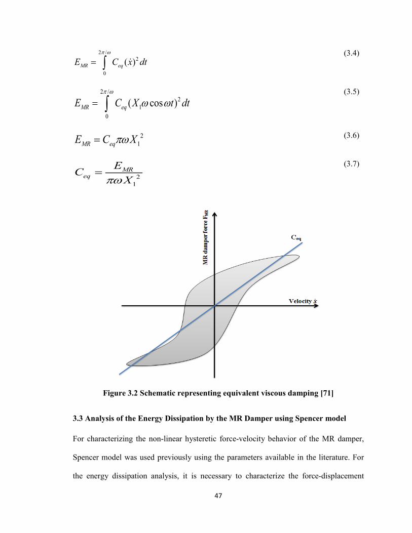
47
(3.4)
(3.5)
(3.6)
(3.7)
Figure 3.2 Schematic representing equivalent viscous damping [71]
3.3 Analysis of the Energy Dissipation by the MR Damper using Spencer model
For characterizing the non-linear hysteretic force-velocity behavior of the MR damper,
Spencer model was used previously using the parameters available in the literature. For
the energy dissipation analysis, it is necessary to characterize the force-displacement
2 /2
0
( )MR eqE C x dtπ ω
= ∫
2 /2
10
( cos )MR eqE C X t dtπ ω
ω ω= ∫
21MR eqE C Xπω=
21
MReq
ECXπω
=
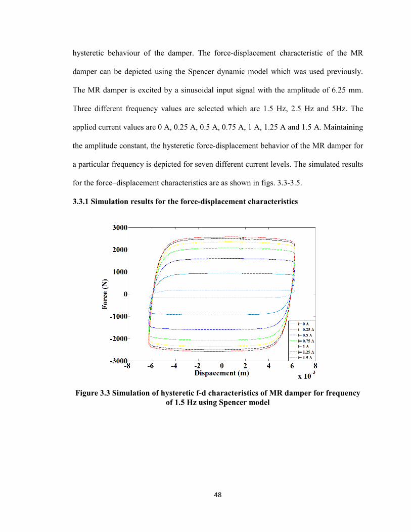
48
hysteretic behaviour of the damper. The force-displacement characteristic of the MR
damper can be depicted using the Spencer dynamic model which was used previously.
The MR damper is excited by a sinusoidal input signal with the amplitude of 6.25 mm.
Three different frequency values are selected which are 1.5 Hz, 2.5 Hz and 5Hz. The
applied current values are 0 A, 0.25 A, 0.5 A, 0.75 A, 1 A, 1.25 A and 1.5 A. Maintaining
the amplitude constant, the hysteretic force-displacement behavior of the MR damper for
a particular frequency is depicted for seven different current levels. The simulated results
for the force–displacement characteristics are as shown in figs. 3.3-3.5.
3.3.1 Simulation results for the force-displacement characteristics
Figure 3.3 Simulation of hysteretic f-d characteristics of MR damper for frequency of 1.5 Hz using Spencer model
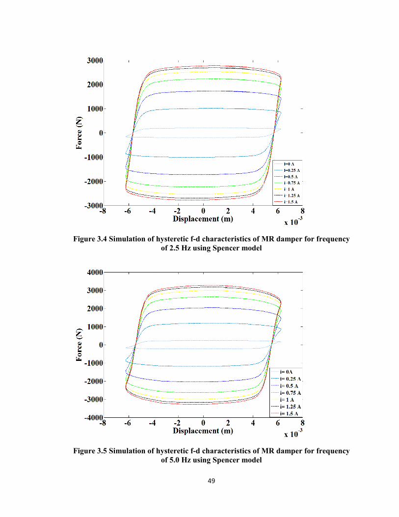
49
Figure 3.4 Simulation of hysteretic f-d characteristics of MR damper for frequency of 2.5 Hz using Spencer model
Figure 3.5 Simulation of hysteretic f-d characteristics of MR damper for frequency of 5.0 Hz using Spencer model
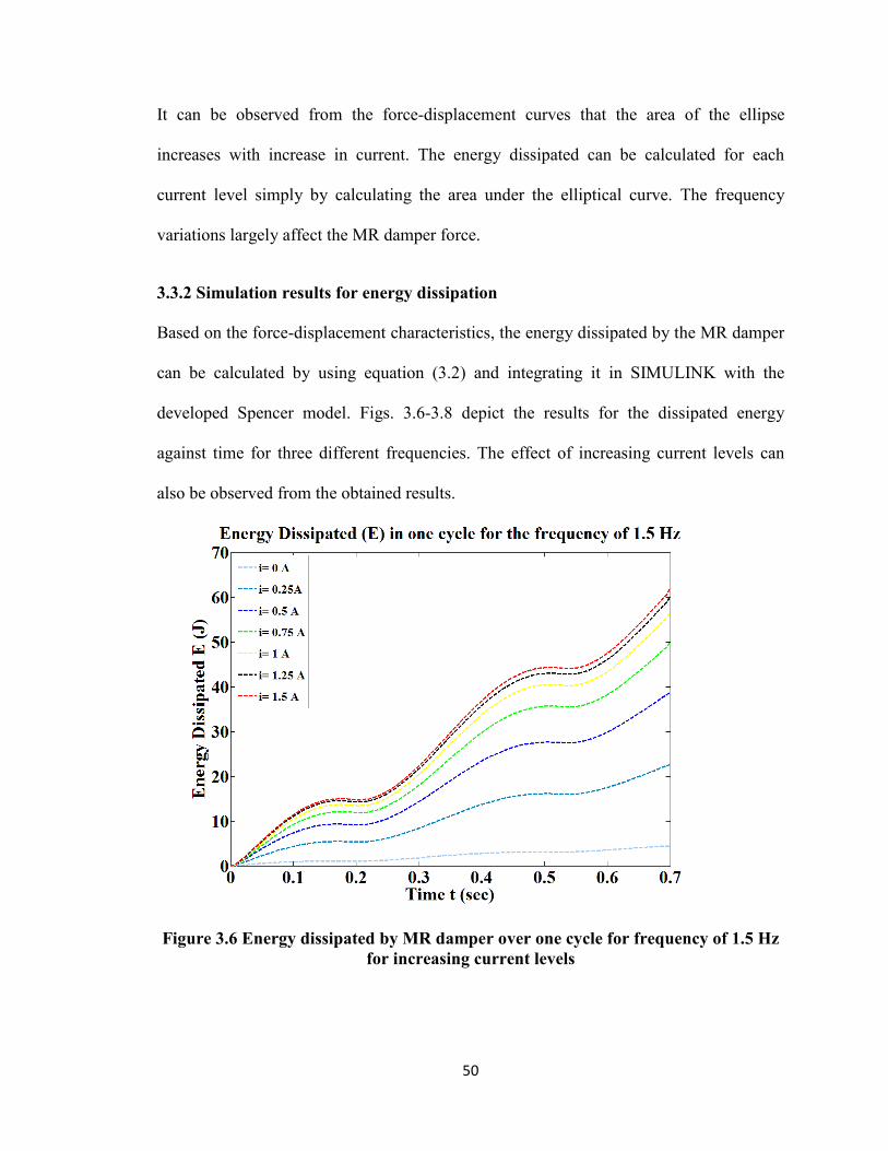
50
It can be observed from the force-displacement curves that the area of the ellipse
increases with increase in current. The energy dissipated can be calculated for each
current level simply by calculating the area under the elliptical curve. The frequency
variations largely affect the MR damper force.
3.3.2 Simulation results for energy dissipation
Based on the force-displacement characteristics, the energy dissipated by the MR damper
can be calculated by using equation (3.2) and integrating it in SIMULINK with the
developed Spencer model. Figs. 3.6-3.8 depict the results for the dissipated energy
against time for three different frequencies. The effect of increasing current levels can
also be observed from the obtained results.
Figure 3.6 Energy dissipated by MR damper over one cycle for frequency of 1.5 Hz for increasing current levels
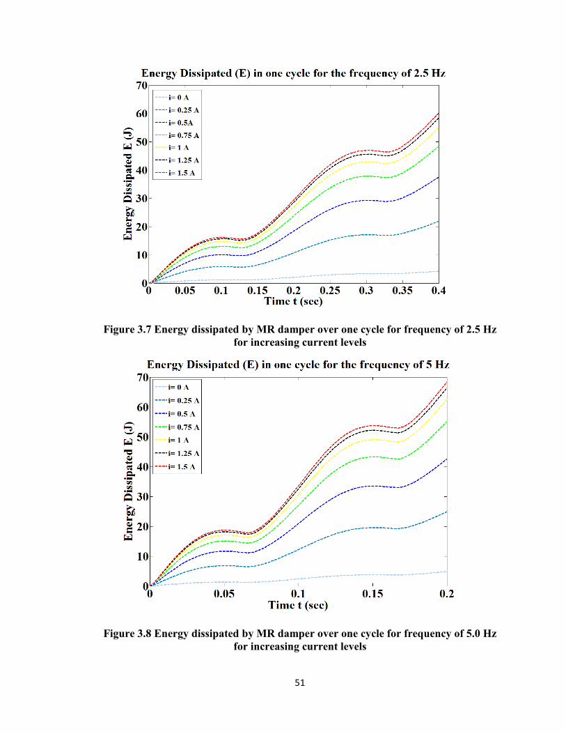
51
Figure 3.7 Energy dissipated by MR damper over one cycle for frequency of 2.5 Hz for increasing current levels
Figure 3.8 Energy dissipated by MR damper over one cycle for frequency of 5.0 Hz for increasing current levels
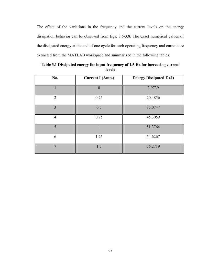
52
The effect of the variations in the frequency and the current levels on the energy
dissipation behavior can be observed from figs. 3.6-3.8. The exact numerical values of
the dissipated energy at the end of one cycle for each operating frequency and current are
extracted from the MATLAB workspace and summarized in the following tables.
Table 3.1 Dissipated energy for input frequency of 1.5 Hz for increasing current levels
No. Current I (Amp.) Energy Dissipated E (J)
1 0 3.9739
2 0.25 20.4856
3 0.5 35.0747
4 0.75 45.3059
5 1 51.3764
6 1.25 54.6267
7 1.5 56.2719
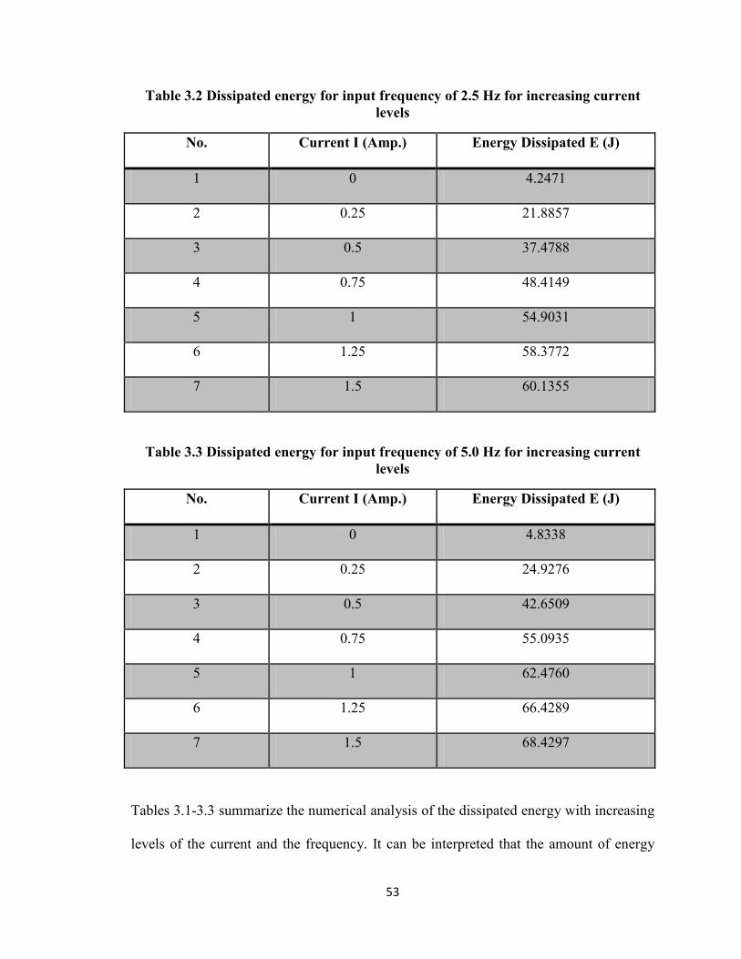
53
Table 3.2 Dissipated energy for input frequency of 2.5 Hz for increasing current levels
No. Current I (Amp.) Energy Dissipated E (J)
1 0 4.2471
2 0.25 21.8857
3 0.5 37.4788
4 0.75 48.4149
5 1 54.9031
6 1.25 58.3772
7 1.5 60.1355
Table 3.3 Dissipated energy for input frequency of 5.0 Hz for increasing current levels
No. Current I (Amp.) Energy Dissipated E (J)
1 0 4.8338
2 0.25 24.9276
3 0.5 42.6509
4 0.75 55.0935
5 1 62.4760
6 1.25 66.4289
7 1.5 68.4297
Tables 3.1-3.3 summarize the numerical analysis of the dissipated energy with increasing
levels of the current and the frequency. It can be interpreted that the amount of energy
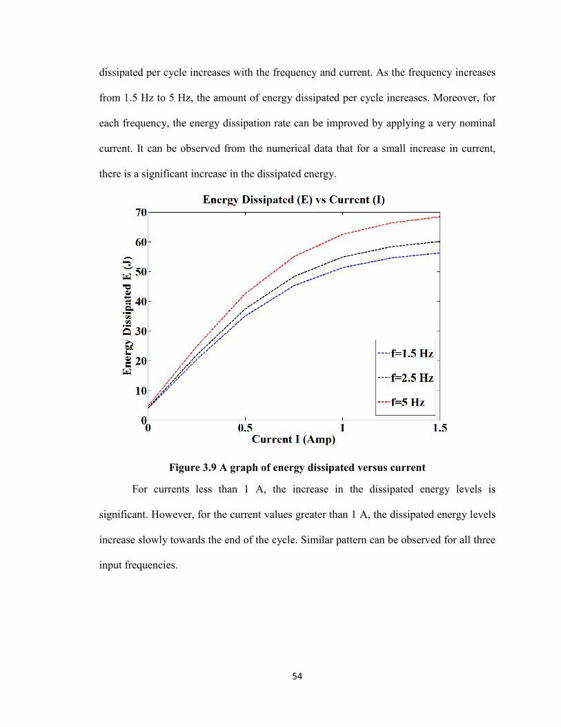
54
dissipated per cycle increases with the frequency and current. As the frequency increases
from 1.5 Hz to 5 Hz, the amount of energy dissipated per cycle increases. Moreover, for
each frequency, the energy dissipation rate can be improved by applying a very nominal
current. It can be observed from the numerical data that for a small increase in current,
there is a significant increase in the dissipated energy.
Figure 3.9 A graph of energy dissipated versus current
For currents less than 1 A, the increase in the dissipated energy levels is
significant. However, for the current values greater than 1 A, the dissipated energy levels
increase slowly towards the end of the cycle. Similar pattern can be observed for all three
input frequencies.
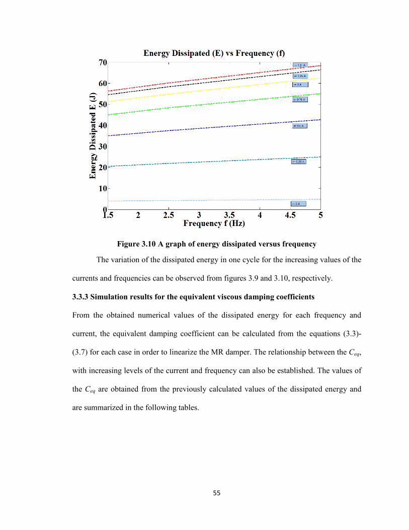
55
Figure 3.10 A graph of energy dissipated versus frequency
The variation of the dissipated energy in one cycle for the increasing values of the
currents and frequencies can be observed from figures 3.9 and 3.10, respectively.
3.3.3 Simulation results for the equivalent viscous damping coefficients
From the obtained numerical values of the dissipated energy for each frequency and
current, the equivalent damping coefficient can be calculated from the equations (3.3)-
(3.7) for each case in order to linearize the MR damper. The relationship between the Ceq,
with increasing levels of the current and frequency can also be established. The values of
the Ceq are obtained from the previously calculated values of the dissipated energy and
are summarized in the following tables.
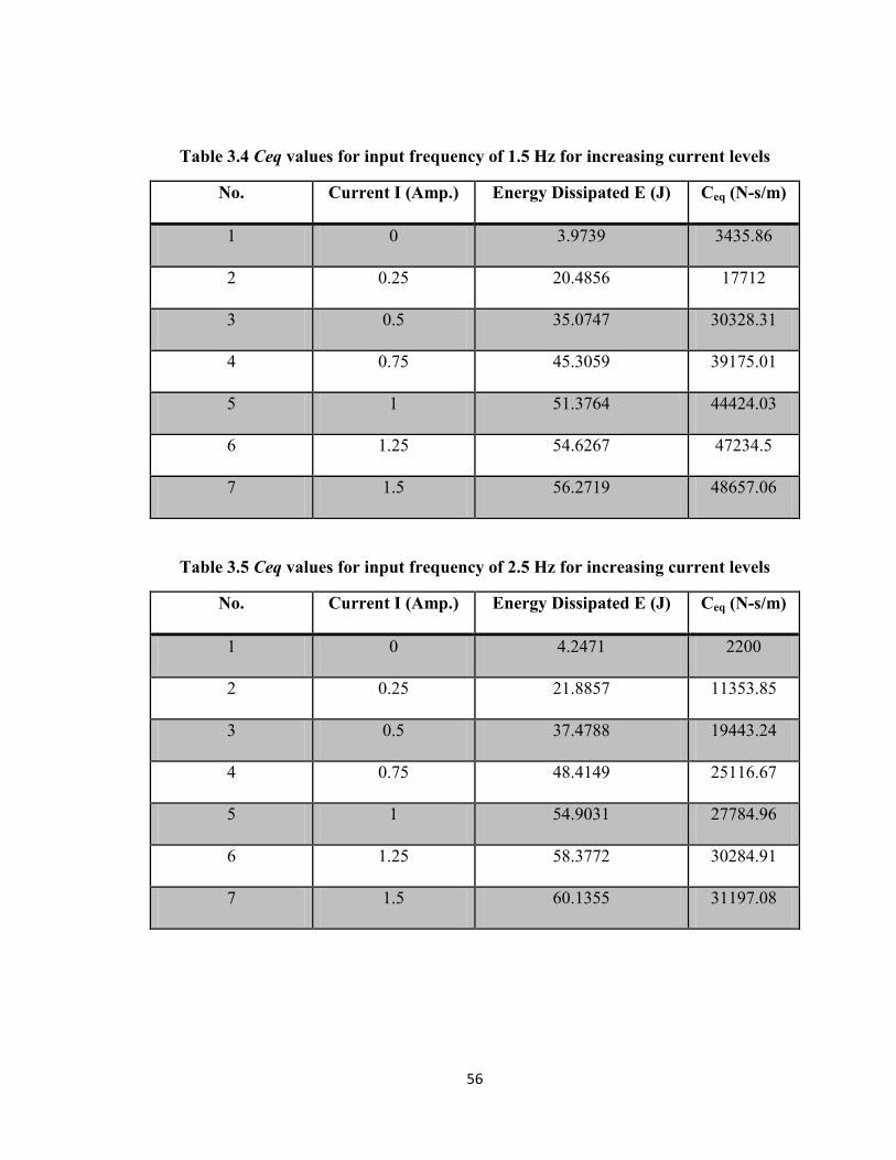
56
Table 3.4 Ceq values for input frequency of 1.5 Hz for increasing current levels
No. Current I (Amp.) Energy Dissipated E (J) Ceq (N-s/m)
1 0 3.9739 3435.86
2 0.25 20.4856 17712
3 0.5 35.0747 30328.31
4 0.75 45.3059 39175.01
5 1 51.3764 44424.03
6 1.25 54.6267 47234.5
7 1.5 56.2719 48657.06
Table 3.5 Ceq values for input frequency of 2.5 Hz for increasing current levels
No. Current I (Amp.) Energy Dissipated E (J) Ceq (N-s/m)
1 0 4.2471 2200
2 0.25 21.8857 11353.85
3 0.5 37.4788 19443.24
4 0.75 48.4149 25116.67
5 1 54.9031 27784.96
6 1.25 58.3772 30284.91
7 1.5 60.1355 31197.08
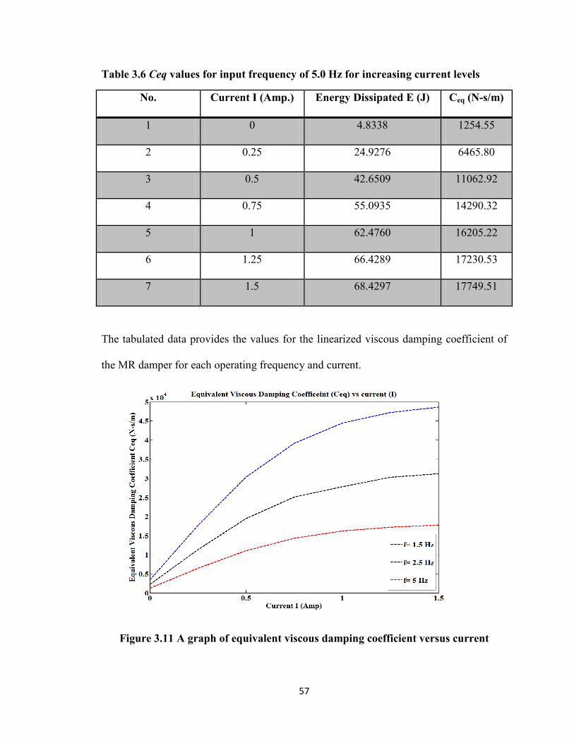
57
Table 3.6 Ceq values for input frequency of 5.0 Hz for increasing current levels
No. Current I (Amp.) Energy Dissipated E (J) Ceq (N-s/m)
1 0 4.8338 1254.55
2 0.25 24.9276 6465.80
3 0.5 42.6509 11062.92
4 0.75 55.0935 14290.32
5 1 62.4760 16205.22
6 1.25 66.4289 17230.53
7 1.5 68.4297 17749.51
The tabulated data provides the values for the linearized viscous damping coefficient of
the MR damper for each operating frequency and current.
Figure 3.11 A graph of equivalent viscous damping coefficient versus current
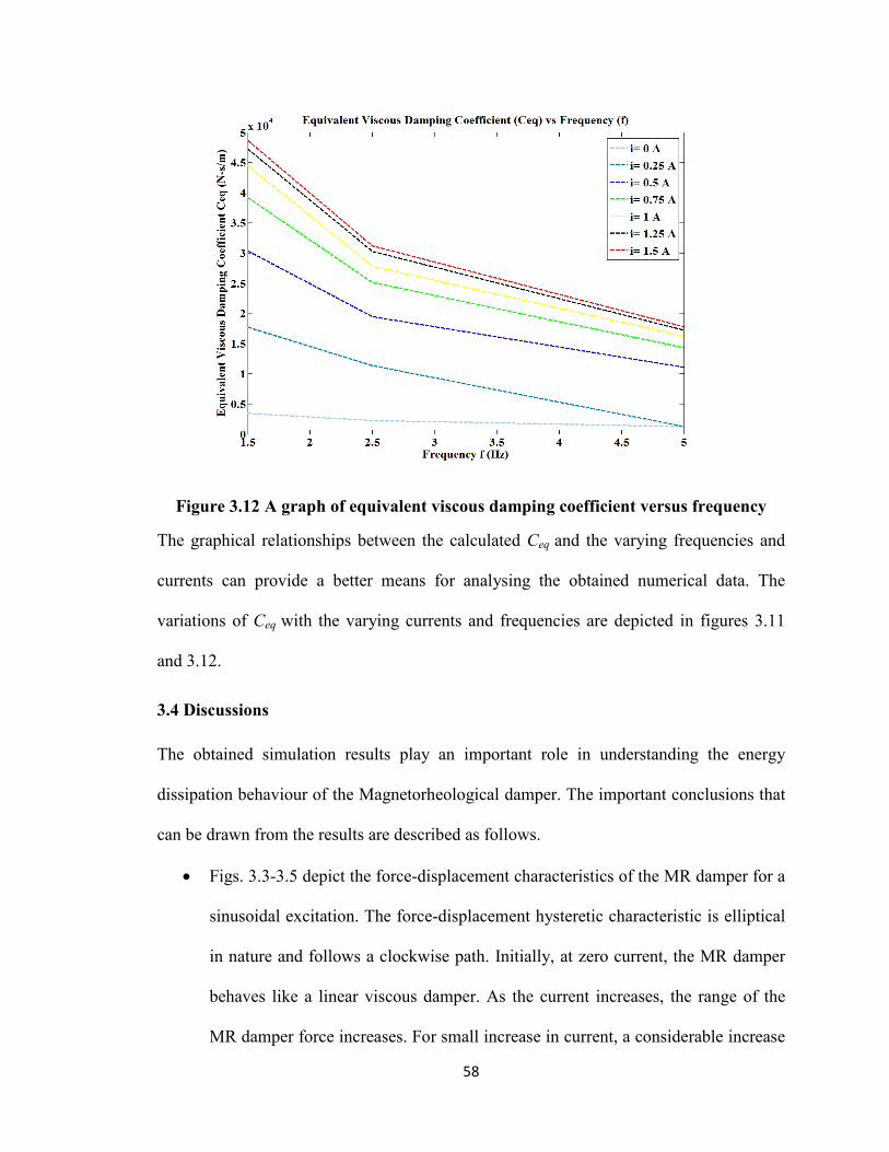
58
Figure 3.12 A graph of equivalent viscous damping coefficient versus frequency
The graphical relationships between the calculated Ceq and the varying frequencies and
currents can provide a better means for analysing the obtained numerical data. The
variations of Ceq with the varying currents and frequencies are depicted in figures 3.11
and 3.12.
3.4 Discussions
The obtained simulation results play an important role in understanding the energy
dissipation behaviour of the Magnetorheological damper. The important conclusions that
can be drawn from the results are described as follows.
• Figs. 3.3-3.5 depict the force-displacement characteristics of the MR damper for a
sinusoidal excitation. The force-displacement hysteretic characteristic is elliptical
in nature and follows a clockwise path. Initially, at zero current, the MR damper
behaves like a linear viscous damper. As the current increases, the range of the
MR damper force increases. For small increase in current, a considerable increase
59
in the damper force can be observed from the simulation results. It is necessary to
depict the force-displacement characteristics of the MR damper accurately, as this
characteristic is important in calculating the dissipated energy by integrating the
area under the elliptical loop.
• The energy dissipation characteristics of the MR damper for sinusoidal excitations
can be observed from the figs. 3.6-3.8. It can be seen that the amount of energy
dissipated in one cycle increases with increase in frequency. The energy
dissipation curves follow a sinusoidal pattern. The current also has a significant
effect on the dissipated energy. From the numerical values summarized in tables
3.1-3.3, it can be concluded that the rate of energy dissipation increases with
small increase in current levels. The highest amount of energy is dissipated when
the input frequency is 5 Hz and a current of 1.5 A is applied in a circuit.
• From the obtained numerical data, the graphical relationships depicting the
variation of the dissipated energy with the increasing current and frequency levels
are plotted which can be seen from figs. 3.9 and 3.10. For each input frequency,
the energy dissipated increases initially linearly for small values of currents.
However, the relationship is no longer linear when the current increases above 0.5
A. A sharp rise in the dissipated energy can be observed for the current levels
smaller than 1 A. As soon as the current increases above 1 A, the rise in the
dissipated energy is not sharp towards the end of the cycle. Figure 3.10 depicts the
plot of the dissipated energy against the frequency variations. The energy
dissipation behaviour follows a linear pattern with increasing frequencies.
60
The numerical values of the calculated equivalent viscous damping coefficients
are presented in tables 3.4-3.6. Based on this numerical data, the graphs of the
equivalent viscous damping coefficient, Ceq, are plotted against the increasing
levels of the current and the frequency. Figure 3.10 depicts the relationship
between the equivalent viscous damping coefficient and the current. For the
highest frequency of 5 Hz, the value of the Ceq obtained is the lowest at 0 A. As
the current increases, the Ceq value also increases for each operating frequency.
The highest values of the Ceq are obtained for the lowest frequency of 1.5 Hz. The
relationship between the varying levels of the frequency and the Ceq can be
observed from figure 3.11.
3.5 Summary
This chapter dealt with the analysis of the energy dissipation behavior of the
Magnetorheological dampers using Spencer model. The basic principles of the energy
dissipation analysis were reviewed initially, followed by deriving the equations for
calculating the dissipated energy over one complete cycle by the MR damper. For this
purpose, the force-displacement characteristics of the MR damper were plotted using
Spencer dynamic model. From the obtained force-displacement characteristics, the
dissipated energy was calculated for each operating frequency and current level. In order
to linearize the MR damper, the equivalent viscous damping coefficients were calculated.
The graphical relationships between the dissipated energy and the varying currents and
frequencies were established.
61
Moreover, the graphs depicting the relationship of the equivalent viscous damping
coefficient with varying frequencies and currents were also plotted.
The results obtained in the present chapter as well as the previous chapter validate
the applicability of the Spencer model for modeling the dynamic behaviour of the MR
dampers. The model could analyze the energy dissipation behaviors which are extremely
important to understand before using the MR dampers for the vibration mitigation
applications.
62
CHAPTER 4
SEMI-ACTIVE CONTROL OF AIRCRAFT LANDING GEAR
SYSTEM USING H∞ AND LINEAR QUADRATIC REGULATOR
(LQR) CONTROL APPROACH
4.1 Introduction
Most of the non-fatal aircraft accidents occur during landing. The landing gear plays an
important role by acting as an intermediate cushioning element between the aircraft body
and the runway. During the touchdown, large magnitude vibrations may get induced in
the aircraft fuselage through the landing gear because of the harsh landing conditions.
The landing gear shock absorbers must absorb the impact kinetic energy to maximum
extent and dissipate this energy as quickly as possible in order to prevent large magnitude
vibrations from getting transmitted to the fuselage. The oleo-pneumatic shock absorbers
used in today’s aircraft are the most efficient means of accomplishing such reduction in
vibrations. Also, they exhibit good rate of energy dissipation. Along with the vertical
energy dissipation during the impact, the landing gear must also be able to provide the
required stability and maneuverability after the impact, which requires variable damping.
However, the oleo-pneumatic shock absorber is unable to provide variable damping.
Consistent attempts have been made to implement the semi-active control strategies in
aircraft landing gears to obtain the improved rate of energy dissipation during landing [1],
[2].
It is evident from the reviewed literature that the semi-active suspension systems
have the advantage over the conventional passive and the active suspension systems.
63
Semi-active systems are robust, easy to build and are more efficient. Moreover, these
systems eliminate the need for high power actuators. In early semi-active suspension
systems, the goal of developing the required damping force could be achieved by varying
the orifice area of the conventional damper thereby resisting the fluid flow according to
the damping requirements. By using the Magnetorheological damper as an actuating
mechanism, an efficient semi-active system can be built as these dampers can provide the
controllable forces for nominal current thereby eliminating the need for large power
supply [86]. Moreover, there are numerous mathematical models available for modeling
the hysteretic dynamic behavior and the energy dissipation behavior of the MR damper.
As evident from the previous chapters, Spencer model could describe the non-linear
dynamic behavior of the MR damper satisfactorily thereby facilitating the design of the
controller.
Various mathematical models of the aircraft system are available for the vibration
analysis depending upon the particular landing gear configuration. Landing gear systems
are classified depending upon the number of wheels carried by each landing gear and the
pattern in which the wheels are arranged. Most of the aircraft have the tri-cycle landing
gear configuration with two main landing gears at the back and one nose landing gear at
the front. The number of wheels per landing gear is dependent on the aircraft weight and
the loading conditions [2] .Hua-Lin et al [20], Wang et al. [27], Sivakumar & Haran [28]
and Zapateiro et al [29], simulated two degrees of freedom (DOFs) aircraft model for the
vibration analysis during landing impact. The advantage of this model is the simplicity
and the ease with which a control strategy can be developed. This model takes into
account only the vertical motion of the aircraft after landing. However, during landing,
64
the aircraft also undergoes pitch and roll motions which must be identified in the analysis
from the stability point of view. Ghiringhelli and Gauldi [61], [60] simulated a multi-
body aircraft model to analyze the response during the impact.
In this chapter, a methodology is developed for building the semi-active MR suspension
for the aircraft landing gear system. A brief description of the contents of this
methodology is as follows.
• Three degrees of freedom (3 DOF) aircraft model is developed that takes into
consideration the bounce, pitch and roll motions of the aircraft during the landing
impact. The aircraft has a tri-cycle landing gear configuration with one wheel per
landing gear.
• Initially, the equations of motion for a 3 DOF aircraft with a passive suspension
system are derived and the vibration analysis is carried out during the landing
impact for different sink velocities. The purpose of this analysis is to validate the
developed model.
• This is followed by the development of a semi-active suspension for a 3 DOF
aircraft model for the purpose of suppressing the excessive fuselage vibrations
during landing. For building the efficient semi-active landing gear suspension,
MR damper is used as an actuation mechanism for generating the required
damping force for each landing scenario and the damper characteristics are
defined by Spencer model. Two different control approaches, namely, the Linear
Quadratic Regulator (LQR) and the robust H∞ are adopted for developing the
semi-active controlled suspension system.
65
4.2 System Dynamics and Modeling
Today’s aircraft are equipped with the conventional oleo-pneumatic dampers which have
a good rate of energy dissipation. However, these dampers are not able to provide
variable damping forces according to the different operating conditions which can reduce
the damper efficiency over its lifetime. The implementation of semi-active dampers in the
aircraft landing gears would be able to provide the variable rate of energy dissipation.
Moreover, by adjusting the damping force to a desirable range, it is possible to control
the excessive vibrations from getting transmitted to the aircraft fuselage, especially
during the landing phase. For other aircraft operational phases such as taxiing, a lower
damping force is sufficient which can be easily adjusted just by reducing the current.
In this study, a 3 DOF aircraft model is developed for the analysis of the dynamic
behavior of the aircraft during the landing impact. As the aircraft has a tri-cycle landing
gear system, it is assumed that the MR damper replaces the conventional oleo-pneumatic
damper in all the three landing gears. According to the methodology suggested by
Batterbee et al [10] for the design of the MR damper based landing gear, the total force
generated inside the damper is a combination of the gas spring force, a viscous damping
force and a controllable MR force. The gas spring force acts as a spring element and also
provides the necessary stiffness in order to support the aircraft weight. The current
flowing inside the magnetic circuit embedded in a damper does not completely magnetize
the full volume of the MR fluid. The volume of the fluid which remains unaffected acts
as a viscous fluid with Newtonian behavior thus providing the viscous damping effect.
By magnetizing the specific volume of the MR fluid, a controllable MR force can be
achieved. This force is the only adjustable damping force which can be achieved
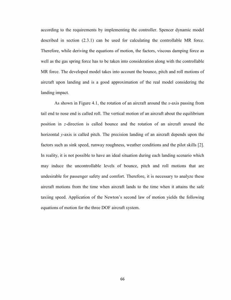
66
according to the requirements by implementing the controller. Spencer dynamic model
described in section (2.3.1) can be used for calculating the controllable MR force.
Therefore, while deriving the equations of motion, the factors, viscous damping force as
well as the gas spring force has to be taken into consideration along with the controllable
MR force. The developed model takes into account the bounce, pitch and roll motions of
aircraft upon landing and is a good approximation of the real model considering the
landing impact.
As shown in Figure 4.1, the rotation of an aircraft around the x-axis passing from
tail end to nose end is called roll. The vertical motion of an aircraft about the equilibrium
position in z-direction is called bounce and the rotation of an aircraft around the
horizontal y-axis is called pitch. The precision landing of an aircraft depends upon the
factors such as sink speed, runway roughness, weather conditions and the pilot skills [2].
In reality, it is not possible to have an ideal situation during each landing scenario which
may induce the uncontrollable levels of bounce, pitch and roll motions that are
undesirable for passenger safety and comfort. Therefore, it is necessary to analyze these
aircraft motions from the time when aircraft lands to the time when it attains the safe
taxiing speed. Application of the Newton’s second law of motion yields the following
equations of motion for the three DOF aircraft system.
67
Figure 4.1 Schematic of 3 DOF aircraft model
(4.1)
(4.2)
(4.3)
where, m, Ix and Iy are the mass of aircraft fuselage, mass moment of inertia about x-axis
and mass moment of inertia about y-axis, respectively. Angle θ represents the angle of
1 1 2 2
3 3 1 1
2 2 3 3
1 2 3
( ) ( )
( ) ( )
( ) ( )
f i r r i
r l i f i
r r i r l i
mz k z l z k z l h zk z l h z c z l z
c z l h z c z l h zF F F
ϕ ϕ θ
ϕ θ ϕ
ϕ θ ϕ θ
+ − − + + − − +
+ + − + − − +
+ − − + + + −= − − −
2 2 3 3
2 2 3 3
3 2
( ) ( )
( ) ( )x r r r i l r l i
r r r i l r l i
l r
I k h z l h z k h z l h z
c h z l h z c h z l h zF h F h
θ ϕ θ ϕ θ
ϕ θ ϕ θ
− + − − − + + −
− + − − − + + −= −
1 1 2 2
3 3 1 1
2 2 3 3
2 3 1
( ) ( )
( ) ( )
( ) ( )( )
y f f i r r r i
r r l i f f i
r r r i r r r i
r f
I k l z l z k l z l h zk l z l h z c l z l z
c l z l h z c l z l h zF F l F l
ϕ ϕ ϕ θ
ϕ θ ϕ
ϕ θ ϕ θ
− − − − + − −
− + + − − − − −
+ − − − + + −= + −
68
roll whereas φ represents the angle of pitch at the time of landing, k1, k2 and k3 represent
the spring constants of the nose landing gear shock absorber, the left main landing gear
shock absorber and the right main landing gear shock absorber, respectively. Constants
c1, c2 and c3 represent the damping coefficients for nose landing gear shock absorber, left
main landing gear shock absorber and right main landing gear shock absorber,
respectively. The distance of the nose landing gear from center of gravity (C.G.) is
represented by lf whereas lr represents the distance of main landing gear from C.G. hl is
the distance of the left main landing gear from the center point and hr is the distance of
the right main landing gear from the center point. The MR damper forces corresponding
to the nose gear, the left main landing gear and the right main landing gear are
represented by F1, F2 and F3, respectively.
4.2.1 Formulation of the MR damper forces
The Magnetorheological damper is implemented as an actuation mechanism for
developing the semi-active suspension system. The MR damper generates the required
forces according to the operating conditions. The MR damper forces F1, F2 and F3 in
equations (4.1)-(4.3), correspond to the nose gear, the left main gear and the right main
gear and act as control input. To formulate the MR damper force in each landing gear,
Spencer dynamic model is used. The dynamic equations of the model are derived as
explained in section 2.3.1 and the parameters are selected from [87] for describing the
dynamic behavior of the MR damper. Spencer model described by Yang et al [87] has a
large force producing capacity of 200 KN. Since the required forces for absorbing the
high impact energy during the aircraft landing are higher, a large capacity MR damper
model is selected in order to build an efficient semi-active landing gear suspension.
69
However, for accurately predicting the MR damper behaviour, Yang et al [87] adopted a
curve fitting approach for establishing a relationship between the current and the MR
damper force instead of using the non-linear current function formulated in equation
(2.2). Referring to the model described in section 2.3.1 and in [87], the overall model
formulation can be done as follows.
(4.4)
(4.5)
(4.6)
3 2( ) 16566 87071 168326 15114i i i iα = − + + (4.7)
3 20 ( ) 437097 1545407 1641376 457741c i i i i= − + + (4.8)
3 2( ) 936310 5334183 48788640 2791630rc i i i i= − + + − (4.9)
The force generated by the MR dampers embedded in the main gears and the nose
gear is given by equation (4.4) which depends on the parameters α, c0 and cr. As
explained previously, the parameter related to the MR fluid yield stress is designated by α
and it is a third order polynomial function of current which is presented in equation (4.7).
The viscous damping coefficient at larger velocities is represented by c0. The dashpot
represented by cr is included in the model to account for the roll-off effect, which is
observed at low velocities. The relationship between the damping coefficient c0 and cr
and the current i is represented by the third order polynomial function as shown in
equations (4.8) and (4.9), respectively. The parameters of the selected Spencer model are
summarized in the following table.
0 0( ) ( ) ( )iD rF p c z q k z q k z zα= + − + − + −
11( ) ( )n np p p z q z q p A z qγ β−= − − − − + −
( )0 00
( )1
rq p c k z qz
c cα= + + −
+
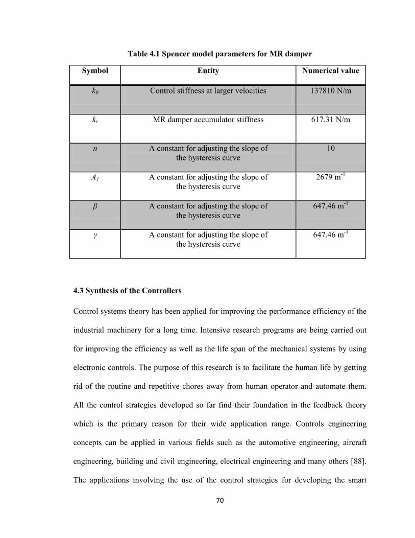
70
Table 4.1 Spencer model parameters for MR damper
Symbol Entity Numerical value
k0 Control stiffness at larger velocities 137810 N/m
kr MR damper accumulator stiffness 617.31 N/m
n A constant for adjusting the slope of the hysteresis curve
10
A1 A constant for adjusting the slope of the hysteresis curve
2679 m-1
β A constant for adjusting the slope of the hysteresis curve
647.46 m-1
γ A constant for adjusting the slope of the hysteresis curve
647.46 m-1
4.3 Synthesis of the Controllers
Control systems theory has been applied for improving the performance efficiency of the
industrial machinery for a long time. Intensive research programs are being carried out
for improving the efficiency as well as the life span of the mechanical systems by using
electronic controls. The purpose of this research is to facilitate the human life by getting
rid of the routine and repetitive chores away from human operator and automate them.
All the control strategies developed so far find their foundation in the feedback theory
which is the primary reason for their wide application range. Controls engineering
concepts can be applied in various fields such as the automotive engineering, aircraft
engineering, building and civil engineering, electrical engineering and many others [88].
The applications involving the use of the control strategies for developing the smart
71
dampers for the vehicles and civil structures have gained a tremendous importance in
recent past. A few implementations of the control strategies for developing the smart
aircraft suspensions have also been reported. However, none of the aircraft has been
equipped with such system till date.
In reality, the mechanical systems are represented in the form of mathematical
models for the ease of analysis. The model cannot predict the behavior of the actual
system accurately. In case of uncertainties in the operating conditions, the behavior of the
model can be different from the actual system. This fact has to be taken into
consideration while designing the control laws for a particular system which accounts for
the robustness analysis. Robustness refers to the stability of the system under
disturbances. Therefore, it is necessary to develop a robust controller for the system in
order to predict its behavior as accurately as possible under varying disturbances in actual
practice [89].
Linear quadratic regulator (LQR) and the H∞ control strategies are amongst the
most widely used control strategies for developing the semi-active suspension system for
road vehicles [90]-[92]. Kumar and Vijayarangan [91] implemented the LQR controller
for a quarter car model by considering the ride quality, road holding and suspension
travel as the performance criterion. Similar approach can also be implemented to design a
semi-active landing gear system for aircraft. Son et al. [93] used a model based H∞
controller for semi-active vehicle suspension to improve ride quality for irregular road
disturbances and proved the effectiveness of H∞ controller for reducing the vertical
accelerations of a sprung mass over wide range of excitation conditions. In addition, the
application of the robust controller for developing a shimmy damper was also reported
72
[94]. The H∞ controller also proved to be a better control strategy for a semi-active
landing gear suspension [29] because of its ability to deal with the uncertainties and
nonlinearities in a systematic way.
In this analysis, two control approaches namely, the linear quadratic regulator
(LQR) and the H∞ are adopted for controlling the bounce of the landing aircraft subjected
to disturbances for the purpose of improving the landing performance during each
landing scenario for the passenger safety. During each landing scenario, the vibrations are
inevitably transferred to the fuselage which may affect passenger safety. The
transmissibility of vibrations depends upon the effectiveness of the damper. The
performance of the passive damper is poor during hard landing scenarios. The semi-
active controlled suspension system can reduce the fuselage vibrations for larger sink
velocities during hard landing scenarios. The controller approaches aim at minimizing the
bounce velocity of the fuselage. For facilitating the formulation of the design of the
controllers, a state-space approach is adopted which is explained in the following section.
4.3.1 Formulation of the H∞ controller using state-space approach
For the systems involving complicated dynamics, the task of controller design becomes
critical. A state-space modeling approach can provide a solution to simplify the
complicated dynamics for the ease of controller design. The state-space approach is a
time domain modeling which can be applied to multivariable systems and also time-
variant systems. The basic principle behind this modeling technique is to represent a
physical system as a set of first order differential equations. The state of a system
describes the condition of that system at any given time. For describing the dynamic
behavior of a system at any given time, it is necessary to represent the system as a set of
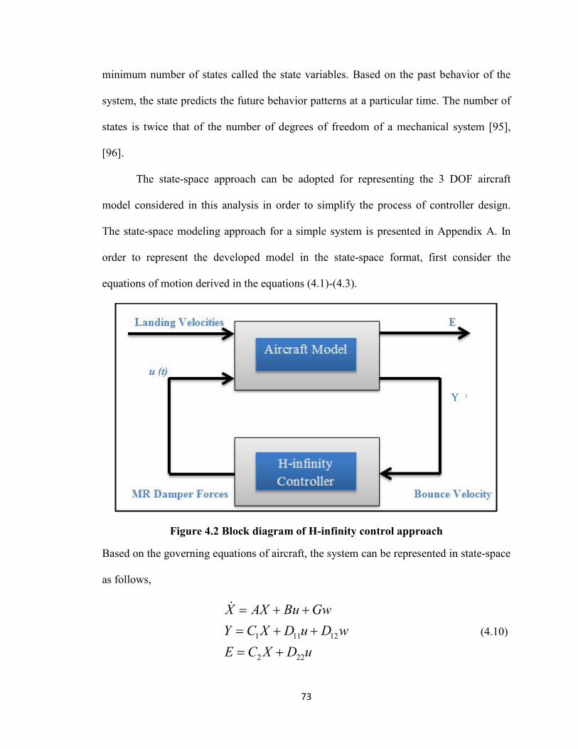
73
minimum number of states called the state variables. Based on the past behavior of the
system, the state predicts the future behavior patterns at a particular time. The number of
states is twice that of the number of degrees of freedom of a mechanical system [95],
[96].
The state-space approach can be adopted for representing the 3 DOF aircraft
model considered in this analysis in order to simplify the process of controller design.
The state-space modeling approach for a simple system is presented in Appendix A. In
order to represent the developed model in the state-space format, first consider the
equations of motion derived in the equations (4.1)-(4.3).
Figure 4.2 Block diagram of H-infinity control approach
Based on the governing equations of aircraft, the system can be represented in state-space
as follows,
(4.10) 1 11 12
2 22
X AX Bu GwY C X D u D wE C X D u
= + += + += +
Y
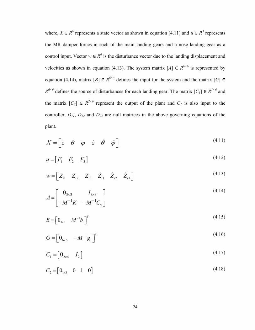
74
where, X ∈ R6 represents a state vector as shown in equation (4.11) and u ∈ R3 represents
the MR damper forces in each of the main landing gears and a nose landing gear as a
control input. Vector w ∈ R6 is the disturbance vector due to the landing displacement and
velocities as shown in equation (4.13). The system matrix [A] ∈ R6×6 is represented by
equation (4.14), matrix [B] ∈ R6×3 defines the input for the system and the matrix [G] ∈
R6×6 defines the source of disturbances for each landing gear. The matrix [C1] ∈ R1×6 and
the matrix [C2] ∈ R2×6 represent the output of the plant and C1 is also input to the
controller, D11, D12 and D22 are null matrices in the above governing equations of the
plant.
(4.11)
[ ]1 2 3u F F F= (4.12)
1 2 3 1 2 3i i i i i iw Z Z Z Z Z Z =
(4.13)
3 3 3 31 1
0
v
IA
M K M C× ×− −
=
− −
(4.14)
13 3 10
TB M b−
× = (4.15)
16 6 10
TG M g−
× = − (4.16)
[ ]1 2 4 20C I×= (4.17)
[ ]2 1 30 0 1 0C ×= (4.18)
X z zθ ϕ θ ϕ =
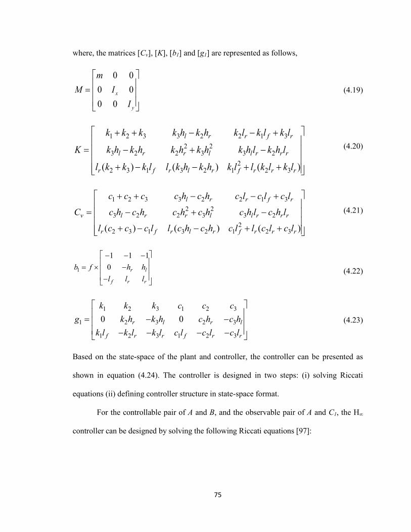
75
where, the matrices [Cv], [K], [b1] and [g1] are represented as follows,
0 00 00 0
x
y
mM I
I
=
(4.19)
1 2 3 3 2 2 1 32 2
3 2 2 3 3 22
2 3 1 3 2 1 2 3( ) ( ) ( )
l r r f r
l r r l l r r r
r f r l r f r r r
k k k k h k h k l k l k l
K k h k h k h k h k h l k h l
l k k k l l k h k h k l l k l k l
+ + − − +
= − + −
+ − − + +
(4.20)
1 2 3 3 2 2 1 32 2
3 2 2 3 3 22
2 3 1 3 2 1 2 3( ) ( ) ( )
l r r f r
v l r r l l r r r
r f r l r f r r r
c c c c h c h c l c l c l
C c h c h c h c h c h l c h l
l c c c l l c h c h c l l c l c l
+ + − − +
= − + −
+ − − + +
(4.21)
1
1 1 10 r l
f r r
b f h hl l l
− − − = × − −
(4.22)
1 2 3 1 2 3
1 2 3 2 3
1 2 3 1 2 3
0 0r l r l
f r r f r r
k k k c c cg k h k h c h c h
k l k l k l c l c l c l
= − − − − − −
(4.23)
Based on the state-space of the plant and controller, the controller can be presented as
shown in equation (4.24). The controller is designed in two steps: (i) solving Riccati
equations (ii) defining controller structure in state-space format.
For the controllable pair of A and B, and the observable pair of A and C1, the H∞
controller can be designed by solving the following Riccati equations [97]:
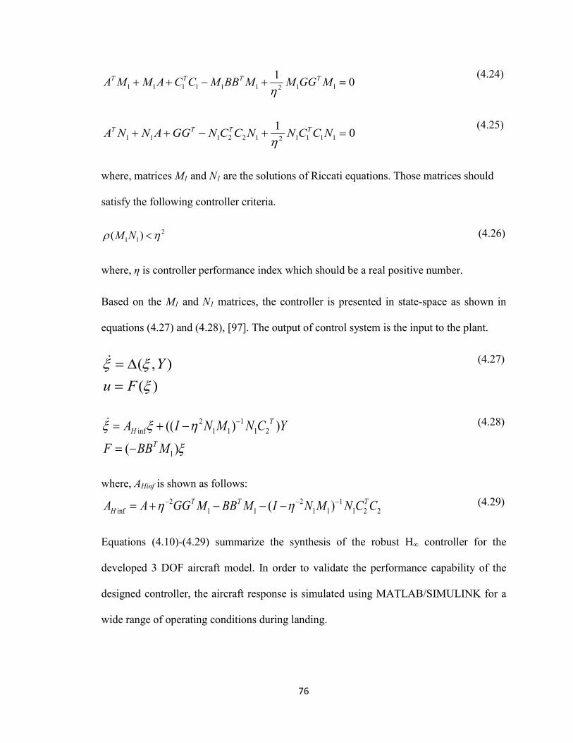
76
(4.24)
(4.25)
where, matrices M1 and N1 are the solutions of Riccati equations. Those matrices should
satisfy the following controller criteria.
(4.26)
where, η is controller performance index which should be a real positive number.
Based on the M1 and N1 matrices, the controller is presented in state-space as shown in
equations (4.27) and (4.28), [97]. The output of control system is the input to the plant.
(4.27)
(4.28)
where, AHinf is shown as follows:
(4.29)
Equations (4.10)-(4.29) summarize the synthesis of the robust H∞ controller for the
developed 3 DOF aircraft model. In order to validate the performance capability of the
designed controller, the aircraft response is simulated using MATLAB/SIMULINK for a
wide range of operating conditions during landing.
1 1 1 1 1 1 1 12
1 0T T T TA M M A C C M BB M M GG Mη
+ + − + =
1 1 1 2 2 1 1 1 1 12
1 0T T T TA N N A GG N C C N N C C Nη
+ + − + =
21 1( )M Nρ η<
( , )( )
Yu Fξ ξ
ξ= ∆=
2 1inf 1 1 1 2
1
(( ) )
( )
TH
T
A I N M N C YF BB Mξ ξ η
ξ
−= + −
= −
2 2 1inf 1 1 1 1 1 2 2( )T T T
HA A GG M BB M I N M N C Cη η− − −= + − − −
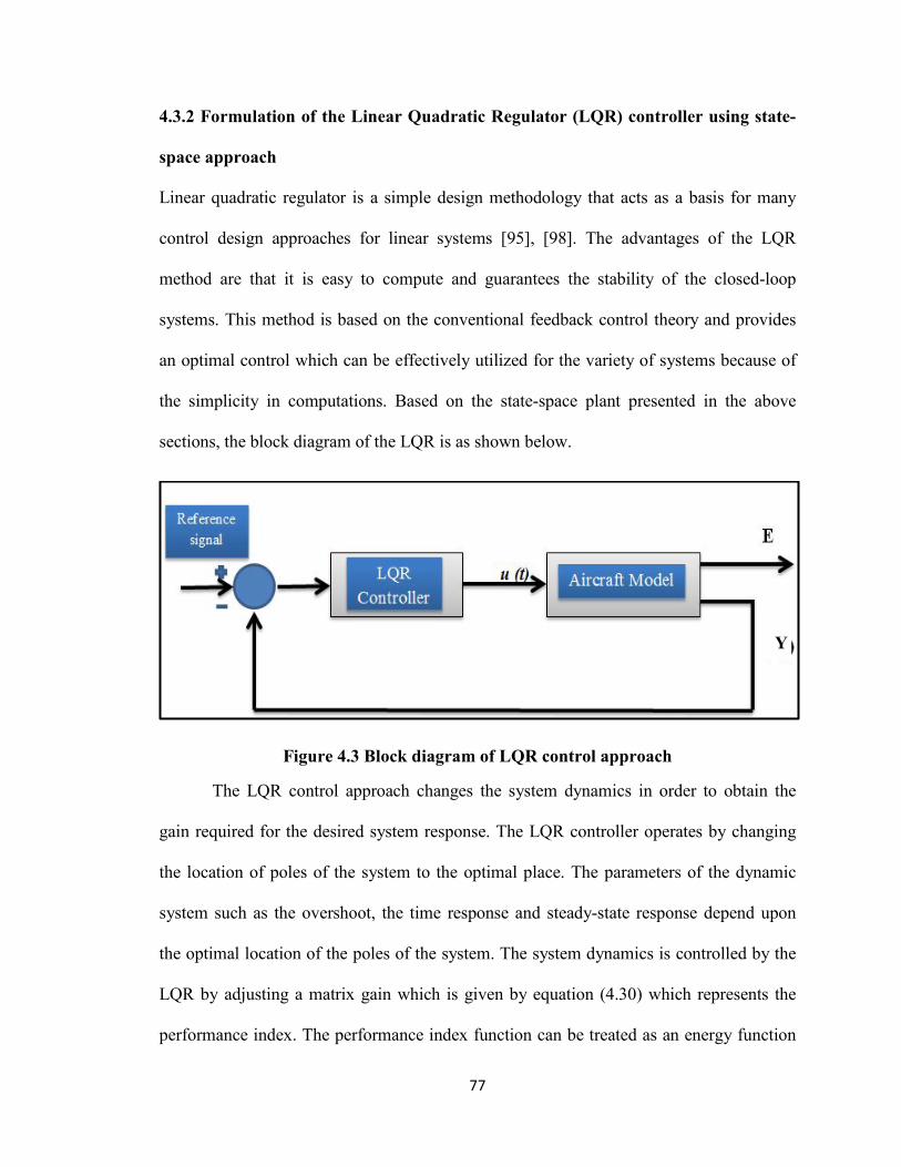
77
4.3.2 Formulation of the Linear Quadratic Regulator (LQR) controller using state-
space approach
Linear quadratic regulator is a simple design methodology that acts as a basis for many
control design approaches for linear systems [95], [98]. The advantages of the LQR
method are that it is easy to compute and guarantees the stability of the closed-loop
systems. This method is based on the conventional feedback control theory and provides
an optimal control which can be effectively utilized for the variety of systems because of
the simplicity in computations. Based on the state-space plant presented in the above
sections, the block diagram of the LQR is as shown below.
Figure 4.3 Block diagram of LQR control approach
The LQR control approach changes the system dynamics in order to obtain the
gain required for the desired system response. The LQR controller operates by changing
the location of poles of the system to the optimal place. The parameters of the dynamic
system such as the overshoot, the time response and steady-state response depend upon
the optimal location of the poles of the system. The system dynamics is controlled by the
LQR by adjusting a matrix gain which is given by equation (4.30) which represents the
performance index. The performance index function can be treated as an energy function
Y
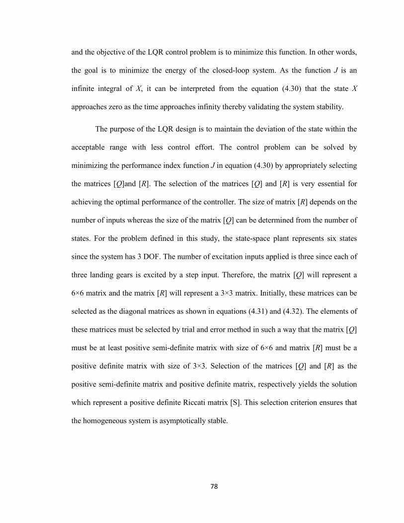
78
and the objective of the LQR control problem is to minimize this function. In other words,
the goal is to minimize the energy of the closed-loop system. As the function J is an
infinite integral of X, it can be interpreted from the equation (4.30) that the state X
approaches zero as the time approaches infinity thereby validating the system stability.
The purpose of the LQR design is to maintain the deviation of the state within the
acceptable range with less control effort. The control problem can be solved by
minimizing the performance index function J in equation (4.30) by appropriately selecting
the matrices [Q]and [R]. The selection of the matrices [Q] and [R] is very essential for
achieving the optimal performance of the controller. The size of matrix [R] depends on the
number of inputs whereas the size of the matrix [Q] can be determined from the number of
states. For the problem defined in this study, the state-space plant represents six states
since the system has 3 DOF. The number of excitation inputs applied is three since each of
three landing gears is excited by a step input. Therefore, the matrix [Q] will represent a
6×6 matrix and the matrix [R] will represent a 3×3 matrix. Initially, these matrices can be
selected as the diagonal matrices as shown in equations (4.31) and (4.32). The elements of
these matrices must be selected by trial and error method in such a way that the matrix [Q]
must be at least positive semi-definite matrix with size of 6×6 and matrix [R] must be a
positive definite matrix with size of 3×3. Selection of the matrices [Q] and [R] as the
positive semi-definite matrix and positive definite matrix, respectively yields the solution
which represent a positive definite Riccati matrix [S]. This selection criterion ensures that
the homogeneous system is asymptotically stable.
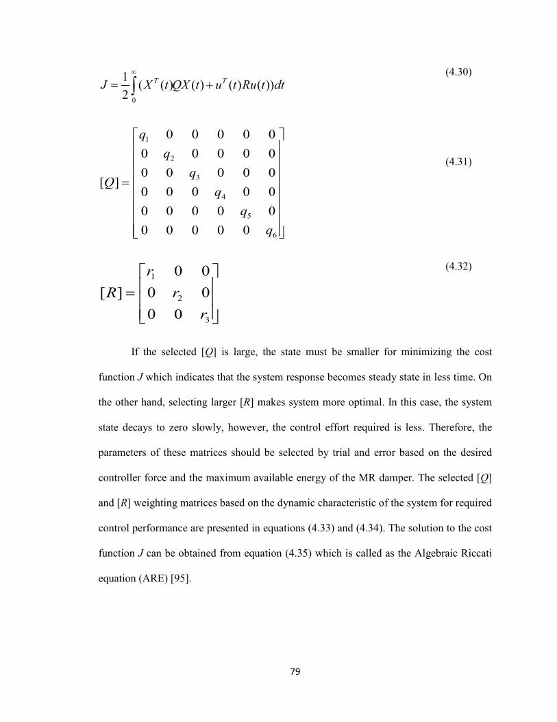
79
(4.30)
(4.31)
(4.32)
If the selected [Q] is large, the state must be smaller for minimizing the cost
function J which indicates that the system response becomes steady state in less time. On
the other hand, selecting larger [R] makes system more optimal. In this case, the system
state decays to zero slowly, however, the control effort required is less. Therefore, the
parameters of these matrices should be selected by trial and error based on the desired
controller force and the maximum available energy of the MR damper. The selected [Q]
and [R] weighting matrices based on the dynamic characteristic of the system for required
control performance are presented in equations (4.33) and (4.34). The solution to the cost
function J can be obtained from equation (4.35) which is called as the Algebraic Riccati
equation (ARE) [95].
0
1 ( ( ) ( ) ( ) ( ))2
T TJ X t QX t u t Ru t dt∞
= +∫
1
2
3
4
5
6
0 0 0 0 00 0 0 0 00 0 0 0 0
[ ]0 0 0 0 00 0 0 0 00 0 0 0 0
q
=
1
2
3
0 0[ ] 0 0
0 0
rR r
r
=
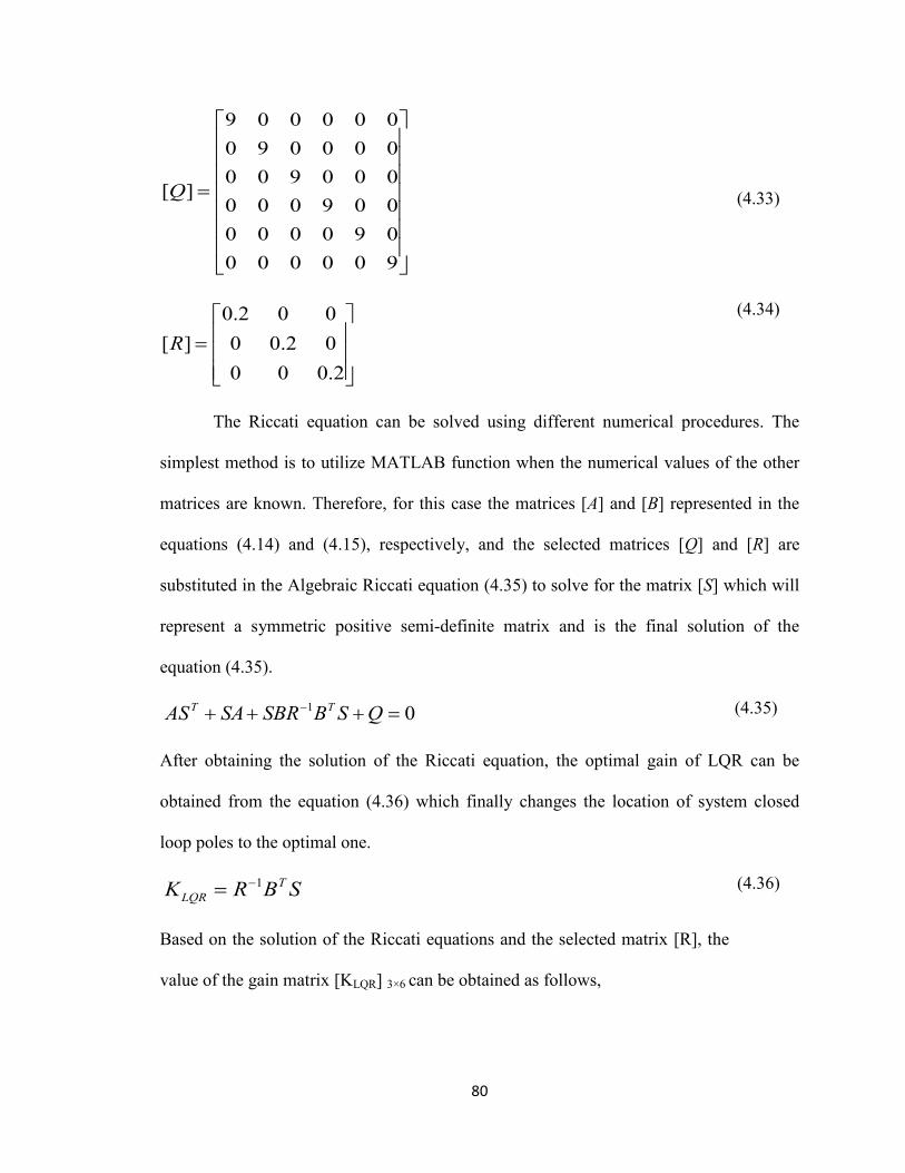
80
(4.33)
(4.34)
The Riccati equation can be solved using different numerical procedures. The
simplest method is to utilize MATLAB function when the numerical values of the other
matrices are known. Therefore, for this case the matrices [A] and [B] represented in the
equations (4.14) and (4.15), respectively, and the selected matrices [Q] and [R] are
substituted in the Algebraic Riccati equation (4.35) to solve for the matrix [S] which will
represent a symmetric positive semi-definite matrix and is the final solution of the
equation (4.35).
1 0T TAS SA SBR B S Q−+ + + = (4.35)
After obtaining the solution of the Riccati equation, the optimal gain of LQR can be
obtained from the equation (4.36) which finally changes the location of system closed
loop poles to the optimal one.
1 TLQRK R B S−=
(4.36)
Based on the solution of the Riccati equations and the selected matrix [R], the
value of the gain matrix [KLQR] 3×6 can be obtained as follows,
9 0 0 0 0 00 9 0 0 0 00 0 9 0 0 0
[ ]0 0 0 9 0 00 0 0 0 9 00 0 0 0 0 9
Q
=
0.2 0 0[ ] 0 0.2 0
0 0 0.2R
=
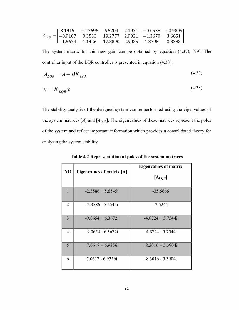
81
KLQR = �3.1915 −1.3696 6.5204 2.1971 −0.0538 −0.9809−0.9107 0.3533 19.2777 2.9021 −1.3670 3.6651−1.5674 1.1426 17.8890 2.9025 1.3795 3.8388
�
The system matrix for this new gain can be obtained by equation (4.37), [99]. The
controller input of the LQR controller is presented in equation (4.38).
LQR LQRA A BK= −
(4.37)
LQRu K x=
(4.38)
The stability analysis of the designed system can be performed using the eigenvalues of
the system matrices [A] and [ALQR]. The eigenvalues of these matrices represent the poles
of the system and reflect important information which provides a consolidated theory for
analyzing the system stability.
Table 4.2 Representation of poles of the system matrices
NO Eigenvalues of matrix [A] Eigenvalues of matrix
[ALQR]
1 -2.3586 + 5.6545i -35.5666
2 -2.3586 - 5.6545i -2.5244
3 -9.0654 + 6.3672i -4.8724 + 5.7544i
4 -9.0654 - 6.3672i -4.8724 - 5.7544i
5 -7.0617 + 6.9356i -8.3016 + 5.3904i
6 7.0617 - 6.9356i -8.3016 - 5.3904i
82
In equation (4.38), KLQR represents the optimal pole placement gain which shifts
the poles of system to the left half plane close to real axis. As long as the poles of the
system are in left half plane, the system is said to be asymptotically stable. For the case
analyzed in this study, it can be observed from the following table that the system poles lie
in left half plane which ensures system stability during landing procedure. Therefore, it
becomes necessary in LQR problem to identify the eigenvalues of the system matrices for
stability analysis under different inputs. The following table identifies the eigenvalues of
the system matrices before and after the application of control.
4.4 Summary
In the presented chapter, the equations of motion for a 3 DOF aircraft model are derived
considering the bounce, pitch and roll motions. A methodology is presented for
developing the semi-active suspension system for the aircraft model implementing two
different control strategies. The landing gear is equipped with the magnetorheological
damper replacing the existing Oleo-pneumatic damper. The MR damper provides an
effective actuation mechanism by providing the required damping forces for different
operating conditions. The dynamic behavior of the MR damper is analyzed using Spencer
model and the parameters of the model are selected from the literature. For designing the
robust controller, a state-space modeling approach is adopted and the mathematical
equations for synthesizing the robust H∞ controller and the LQR controller are derived.
The remaining part of the study will deal with analyzing the performance of the
developed semi-active MR landing gear. In the next chapter, initially, the performance of
the robust H∞ controller is compared with the LQR controller for a particular sink velocity
with the goal of selecting the best control approach amongst the two. Later, the vibration
83
response of the aircraft for the uncertainties during landing is simulated to validate the
applicability of the designed semi-active system in worst landing scenarios.
84
CHAPTER 5
PERFORMANCE ANALYSIS OF THE AIRCRAFT WITH SEMI-
ACTIVE MAGNETORHEOLOGICAL LANDING GEAR
5.1 Introduction
The primary objective of this study is to develop a methodology for designing a semi-
active suspension for the aircraft landing gear for improving the passenger safety during
the aircraft operations. The goal of designing a smart suspension system for the aircraft
landing gear was achieved through the numerical methodologies adopted in the previous
chapters.
This chapter deals with the validation of the designed semi-active system for the
developed 3 DOF model through simulation approach. Initially, the vibration response of
the passive system is compared with the semi-active system designed using both the
control approaches presented in chapter 4 for a particular sink velocity. Later, the
performance of the controllers is compared for the same sink velocity but taking into
consideration the runway unevenness, which would provide a basis for the selection of
the appropriate controller out of the two suggested ones. Once the selection process of the
control approaches is completed, it is used for controlling the vibrations of the aircraft for
higher landing velocities considering the runway roughness and other adverse operating
conditions. Moreover, the analysis also takes into consideration the pilot inaccuracies
which sometimes may cause damage during landing.
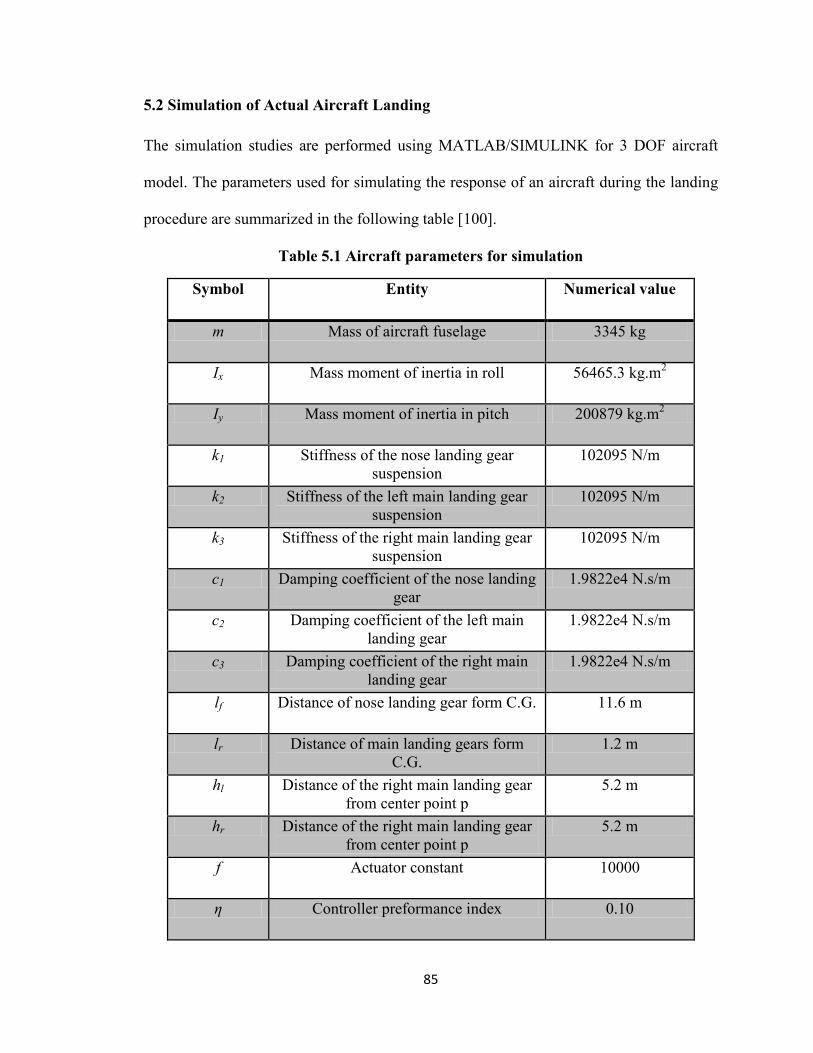
85
5.2 Simulation of Actual Aircraft Landing
The simulation studies are performed using MATLAB/SIMULINK for 3 DOF aircraft
model. The parameters used for simulating the response of an aircraft during the landing
procedure are summarized in the following table [100].
Table 5.1 Aircraft parameters for simulation
Symbol Entity Numerical value
m Mass of aircraft fuselage 3345 kg
Ix Mass moment of inertia in roll 56465.3 kg.m2
Iy Mass moment of inertia in pitch 200879 kg.m2
k1 Stiffness of the nose landing gear suspension
102095 N/m
k2 Stiffness of the left main landing gear suspension
102095 N/m
k3 Stiffness of the right main landing gear suspension
102095 N/m
c1 Damping coefficient of the nose landing gear
1.9822e4 N.s/m
c2 Damping coefficient of the left main landing gear
1.9822e4 N.s/m
c3 Damping coefficient of the right main landing gear
1.9822e4 N.s/m
lf Distance of nose landing gear form C.G. 11.6 m
lr Distance of main landing gears form C.G.
1.2 m
hl Distance of the right main landing gear from center point p
5.2 m
hr Distance of the right main landing gear from center point p
5.2 m
f Actuator constant 10000
η Controller preformance index 0.10
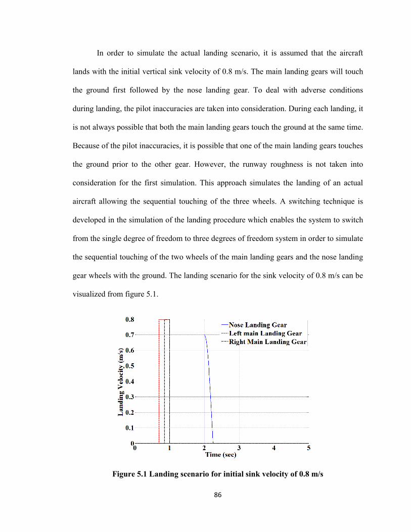
86
In order to simulate the actual landing scenario, it is assumed that the aircraft
lands with the initial vertical sink velocity of 0.8 m/s. The main landing gears will touch
the ground first followed by the nose landing gear. To deal with adverse conditions
during landing, the pilot inaccuracies are taken into consideration. During each landing, it
is not always possible that both the main landing gears touch the ground at the same time.
Because of the pilot inaccuracies, it is possible that one of the main landing gears touches
the ground prior to the other gear. However, the runway roughness is not taken into
consideration for the first simulation. This approach simulates the landing of an actual
aircraft allowing the sequential touching of the three wheels. A switching technique is
developed in the simulation of the landing procedure which enables the system to switch
from the single degree of freedom to three degrees of freedom system in order to simulate
the sequential touching of the two wheels of the main landing gears and the nose landing
gear wheels with the ground. The landing scenario for the sink velocity of 0.8 m/s can be
visualized from figure 5.1.
Figure 5.1 Landing scenario for initial sink velocity of 0.8 m/s
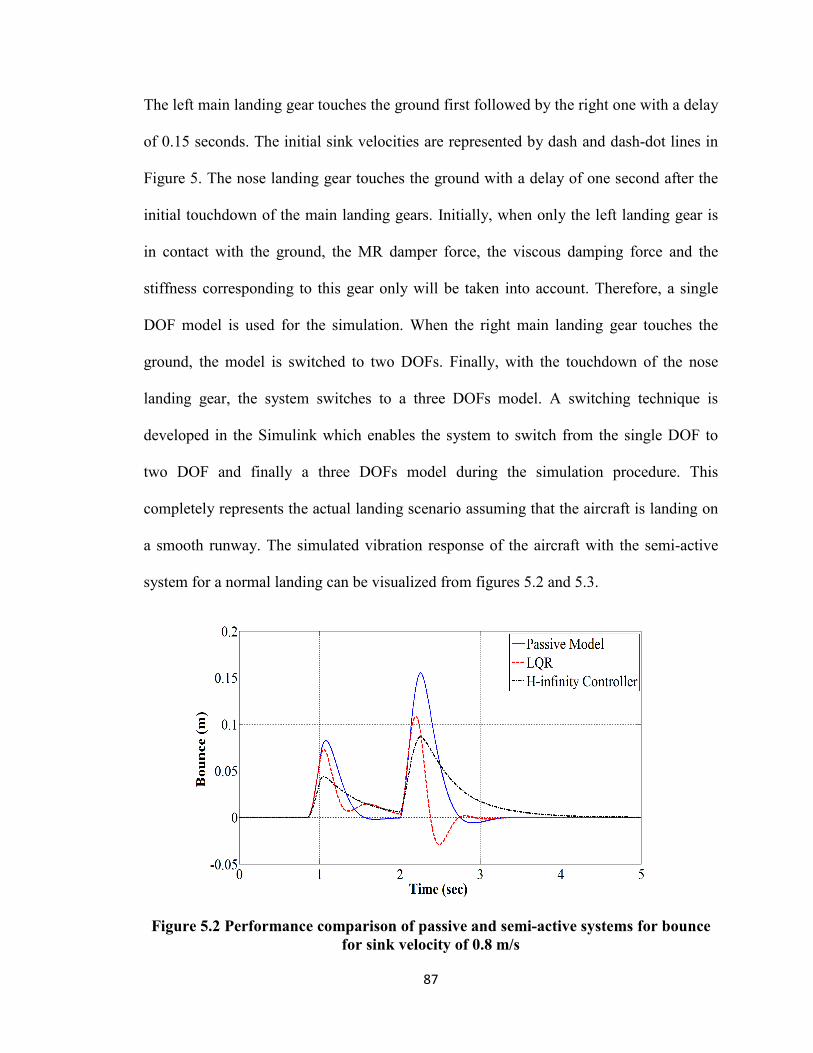
87
The left main landing gear touches the ground first followed by the right one with a delay
of 0.15 seconds. The initial sink velocities are represented by dash and dash-dot lines in
Figure 5. The nose landing gear touches the ground with a delay of one second after the
initial touchdown of the main landing gears. Initially, when only the left landing gear is
in contact with the ground, the MR damper force, the viscous damping force and the
stiffness corresponding to this gear only will be taken into account. Therefore, a single
DOF model is used for the simulation. When the right main landing gear touches the
ground, the model is switched to two DOFs. Finally, with the touchdown of the nose
landing gear, the system switches to a three DOFs model. A switching technique is
developed in the Simulink which enables the system to switch from the single DOF to
two DOF and finally a three DOFs model during the simulation procedure. This
completely represents the actual landing scenario assuming that the aircraft is landing on
a smooth runway. The simulated vibration response of the aircraft with the semi-active
system for a normal landing can be visualized from figures 5.2 and 5.3.
Figure 5.2 Performance comparison of passive and semi-active systems for bounce for sink velocity of 0.8 m/s
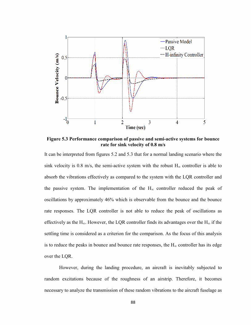
88
Figure 5.3 Performance comparison of passive and semi-active systems for bounce rate for sink velocity of 0.8 m/s
It can be interpreted from figures 5.2 and 5.3 that for a normal landing scenario where the
sink velocity is 0.8 m/s, the semi-active system with the robust H∞ controller is able to
absorb the vibrations effectively as compared to the system with the LQR controller and
the passive system. The implementation of the H∞ controller reduced the peak of
oscillations by approximately 46% which is observable from the bounce and the bounce
rate responses. The LQR controller is not able to reduce the peak of oscillations as
effectively as the H∞. However, the LQR controller finds its advantages over the H∞ if the
settling time is considered as a criterion for the comparison. As the focus of this analysis
is to reduce the peaks in bounce and bounce rate responses, the H∞ controller has its edge
over the LQR.
However, during the landing procedure, an aircraft is inevitably subjected to
random excitations because of the roughness of an airstrip. Therefore, it becomes
necessary to analyze the transmission of these random vibrations to the aircraft fuselage as
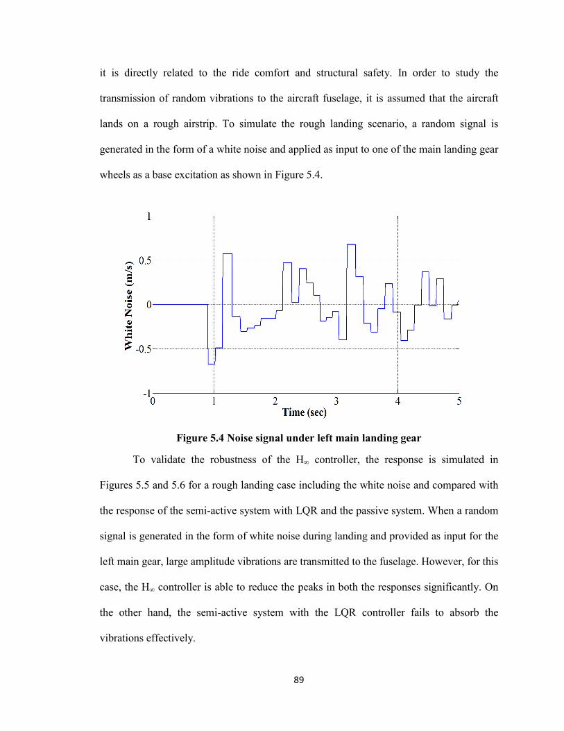
89
it is directly related to the ride comfort and structural safety. In order to study the
transmission of random vibrations to the aircraft fuselage, it is assumed that the aircraft
lands on a rough airstrip. To simulate the rough landing scenario, a random signal is
generated in the form of a white noise and applied as input to one of the main landing gear
wheels as a base excitation as shown in Figure 5.4.
Figure 5.4 Noise signal under left main landing gear
To validate the robustness of the H∞ controller, the response is simulated in
Figures 5.5 and 5.6 for a rough landing case including the white noise and compared with
the response of the semi-active system with LQR and the passive system. When a random
signal is generated in the form of white noise during landing and provided as input for the
left main gear, large amplitude vibrations are transmitted to the fuselage. However, for this
case, the H∞ controller is able to reduce the peaks in both the responses significantly. On
the other hand, the semi-active system with the LQR controller fails to absorb the
vibrations effectively.
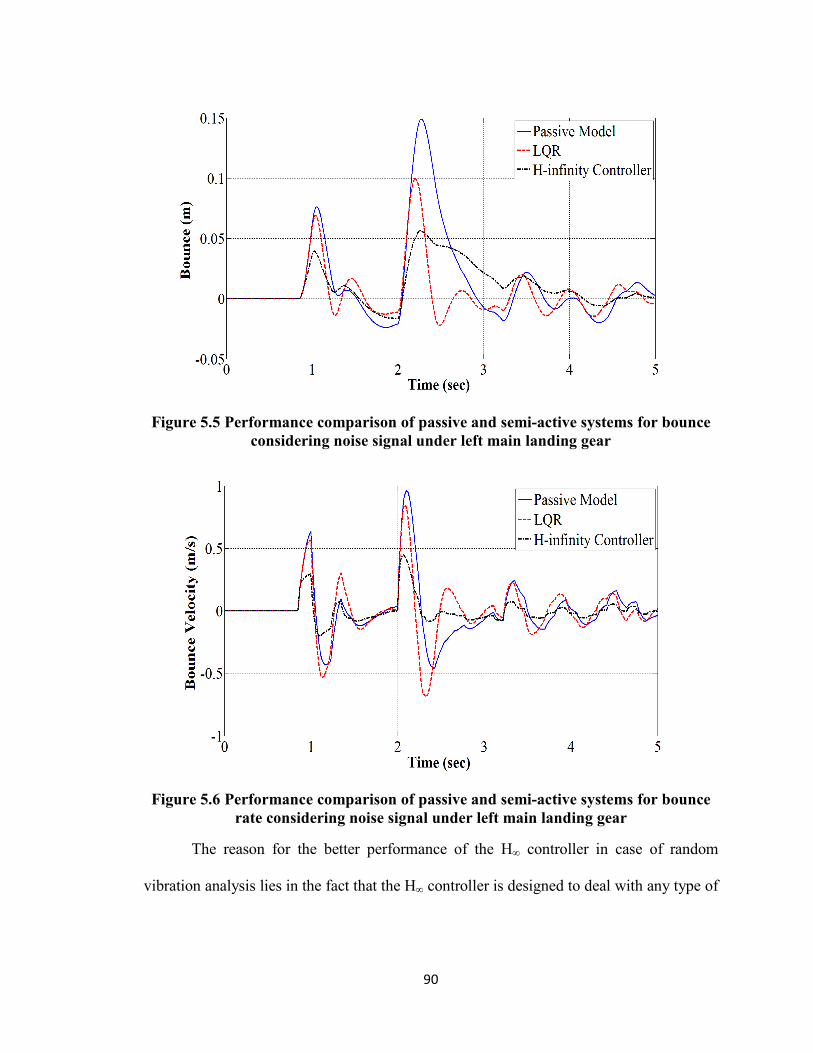
90
Figure 5.5 Performance comparison of passive and semi-active systems for bounce considering noise signal under left main landing gear
Figure 5.6 Performance comparison of passive and semi-active systems for bounce rate considering noise signal under left main landing gear
The reason for the better performance of the H∞ controller in case of random
vibration analysis lies in the fact that the H∞ controller is designed to deal with any type of
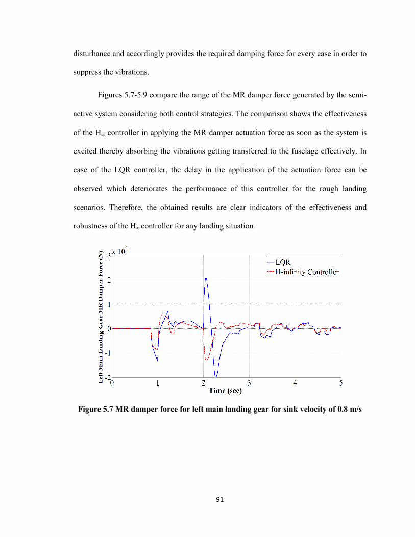
91
disturbance and accordingly provides the required damping force for every case in order to
suppress the vibrations.
Figures 5.7-5.9 compare the range of the MR damper force generated by the semi-
active system considering both control strategies. The comparison shows the effectiveness
of the H∞ controller in applying the MR damper actuation force as soon as the system is
excited thereby absorbing the vibrations getting transferred to the fuselage effectively. In
case of the LQR controller, the delay in the application of the actuation force can be
observed which deteriorates the performance of this controller for the rough landing
scenarios. Therefore, the obtained results are clear indicators of the effectiveness and
robustness of the H∞ controller for any landing situation.
Figure 5.7 MR damper force for left main landing gear for sink velocity of 0.8 m/s
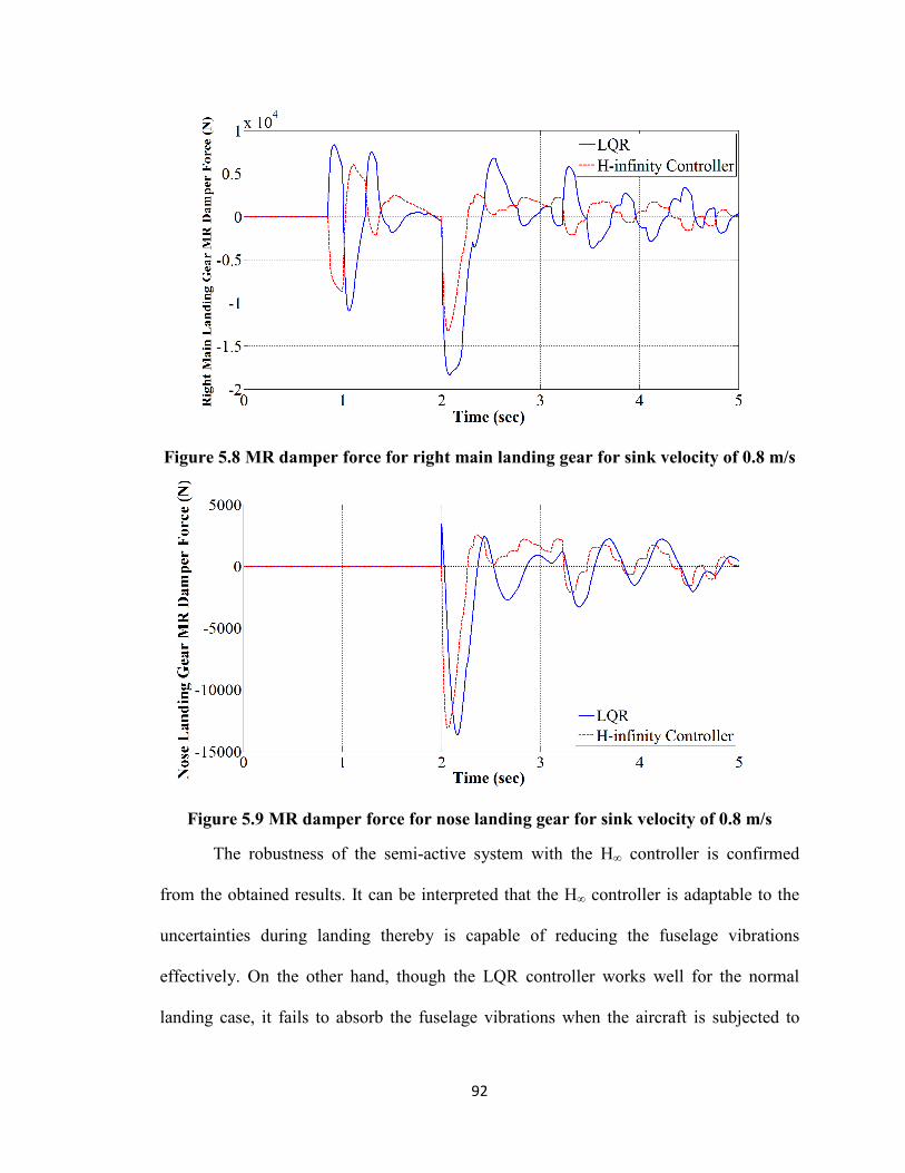
92
Figure 5.8 MR damper force for right main landing gear for sink velocity of 0.8 m/s
Figure 5.9 MR damper force for nose landing gear for sink velocity of 0.8 m/s
The robustness of the semi-active system with the H∞ controller is confirmed
from the obtained results. It can be interpreted that the H∞ controller is adaptable to the
uncertainties during landing thereby is capable of reducing the fuselage vibrations
effectively. On the other hand, though the LQR controller works well for the normal
landing case, it fails to absorb the fuselage vibrations when the aircraft is subjected to
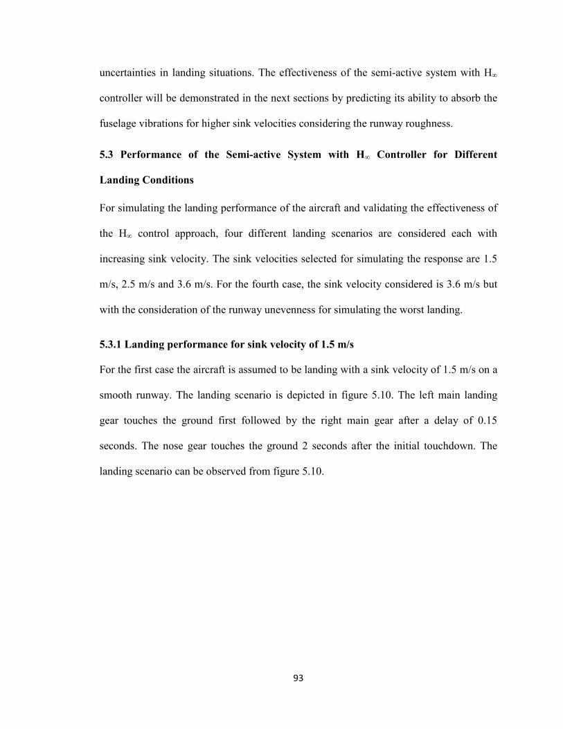
93
uncertainties in landing situations. The effectiveness of the semi-active system with H∞
controller will be demonstrated in the next sections by predicting its ability to absorb the
fuselage vibrations for higher sink velocities considering the runway roughness.
5.3 Performance of the Semi-active System with H∞ Controller for Different
Landing Conditions
For simulating the landing performance of the aircraft and validating the effectiveness of
the H∞ control approach, four different landing scenarios are considered each with
increasing sink velocity. The sink velocities selected for simulating the response are 1.5
m/s, 2.5 m/s and 3.6 m/s. For the fourth case, the sink velocity considered is 3.6 m/s but
with the consideration of the runway unevenness for simulating the worst landing.
5.3.1 Landing performance for sink velocity of 1.5 m/s
For the first case the aircraft is assumed to be landing with a sink velocity of 1.5 m/s on a
smooth runway. The landing scenario is depicted in figure 5.10. The left main landing
gear touches the ground first followed by the right main gear after a delay of 0.15
seconds. The nose gear touches the ground 2 seconds after the initial touchdown. The
landing scenario can be observed from figure 5.10.
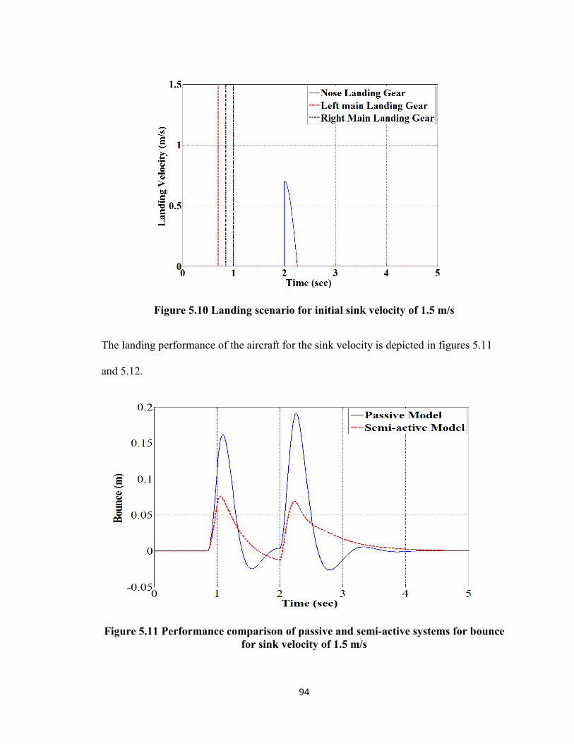
94
Figure 5.10 Landing scenario for initial sink velocity of 1.5 m/s
The landing performance of the aircraft for the sink velocity is depicted in figures 5.11
and 5.12.
Figure 5.11 Performance comparison of passive and semi-active systems for bounce for sink velocity of 1.5 m/s
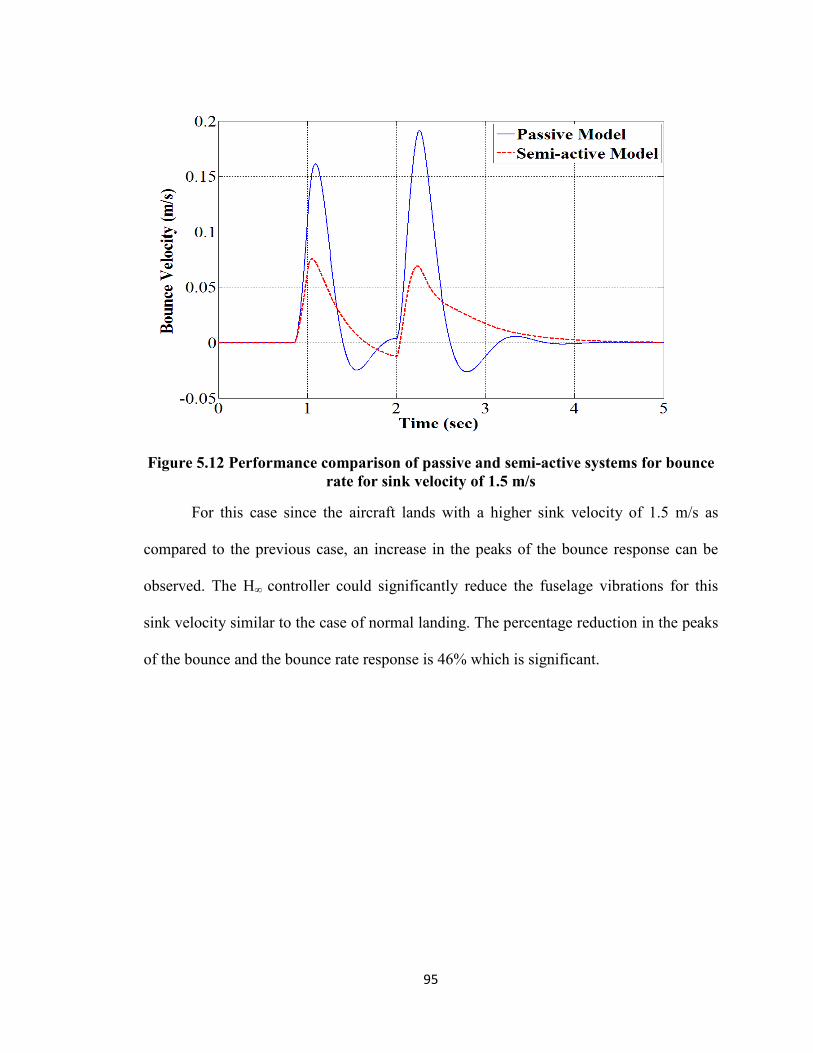
95
Figure 5.12 Performance comparison of passive and semi-active systems for bounce rate for sink velocity of 1.5 m/s
For this case since the aircraft lands with a higher sink velocity of 1.5 m/s as
compared to the previous case, an increase in the peaks of the bounce response can be
observed. The H∞ controller could significantly reduce the fuselage vibrations for this
sink velocity similar to the case of normal landing. The percentage reduction in the peaks
of the bounce and the bounce rate response is 46% which is significant.
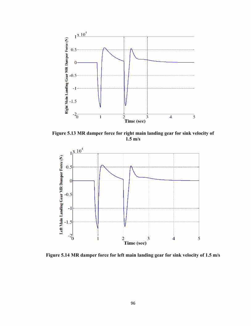
96
Figure 5.13 MR damper force for right main landing gear for sink velocity of 1.5 m/s
Figure 5.14 MR damper force for left main landing gear for sink velocity of 1.5 m/s
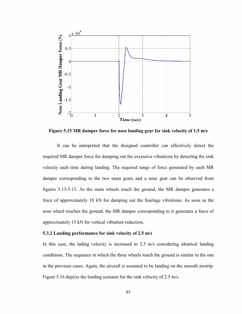
97
Figure 5.15 MR damper force for nose landing gear for sink velocity of 1.5 m/s
It can be interpreted that the designed controller can effectively detect the
required MR damper force for damping out the excessive vibrations by detecting the sink
velocity each time during landing. The required range of force generated by each MR
damper corresponding to the two main gears and a nose gear can be observed from
figures 5.13-5.15. As the main wheels touch the ground, the MR damper generates a
force of approximately 18 kN for damping out the fuselage vibrations. As soon as the
nose wheel touches the ground, the MR damper corresponding to it generates a force of
approximately 15 kN for vertical vibration reduction.
5.3.2 Landing performance for sink velocity of 2.5 m/s
In this case, the lading velocity is increased to 2.5 m/s considering identical landing
conditions. The sequence in which the three wheels touch the ground is similar to the one
in the previous cases. Again, the aircraft is assumed to be landing on the smooth airstrip.
Figure 5.16 depicts the landing scenario for the sink velocity of 2.5 m/s.
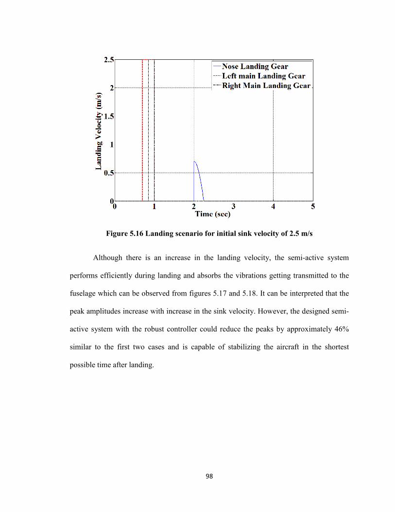
98
Figure 5.16 Landing scenario for initial sink velocity of 2.5 m/s
Although there is an increase in the landing velocity, the semi-active system
performs efficiently during landing and absorbs the vibrations getting transmitted to the
fuselage which can be observed from figures 5.17 and 5.18. It can be interpreted that the
peak amplitudes increase with increase in the sink velocity. However, the designed semi-
active system with the robust controller could reduce the peaks by approximately 46%
similar to the first two cases and is capable of stabilizing the aircraft in the shortest
possible time after landing.
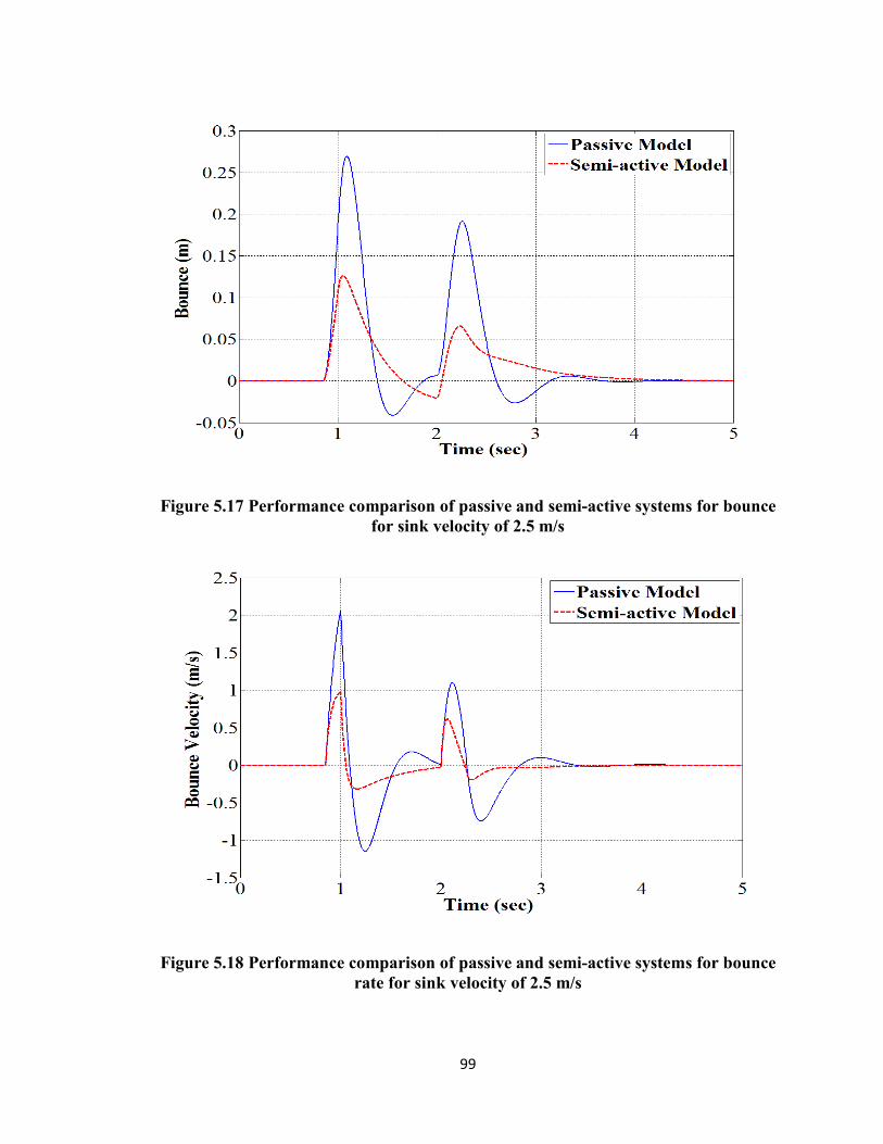
99
Figure 5.17 Performance comparison of passive and semi-active systems for bounce for sink velocity of 2.5 m/s
Figure 5.18 Performance comparison of passive and semi-active systems for bounce rate for sink velocity of 2.5 m/s
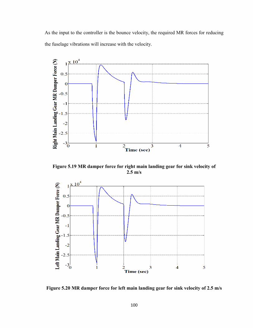
100
As the input to the controller is the bounce velocity, the required MR forces for reducing
the fuselage vibrations will increase with the velocity.
Figure 5.19 MR damper force for right main landing gear for sink velocity of 2.5 m/s
Figure 5.20 MR damper force for left main landing gear for sink velocity of 2.5 m/s
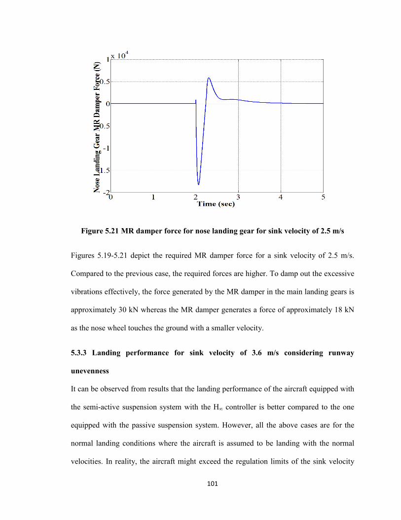
101
Figure 5.21 MR damper force for nose landing gear for sink velocity of 2.5 m/s
Figures 5.19-5.21 depict the required MR damper force for a sink velocity of 2.5 m/s.
Compared to the previous case, the required forces are higher. To damp out the excessive
vibrations effectively, the force generated by the MR damper in the main landing gears is
approximately 30 kN whereas the MR damper generates a force of approximately 18 kN
as the nose wheel touches the ground with a smaller velocity.
5.3.3 Landing performance for sink velocity of 3.6 m/s considering runway
unevenness
It can be observed from results that the landing performance of the aircraft equipped with
the semi-active suspension system with the H∞ controller is better compared to the one
equipped with the passive suspension system. However, all the above cases are for the
normal landing conditions where the aircraft is assumed to be landing with the normal
velocities. In reality, the aircraft might exceed the regulation limits of the sink velocity
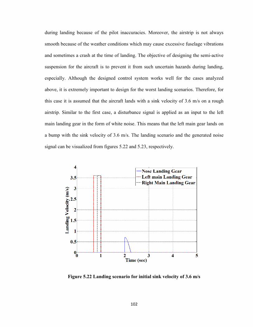
102
during landing because of the pilot inaccuracies. Moreover, the airstrip is not always
smooth because of the weather conditions which may cause excessive fuselage vibrations
and sometimes a crash at the time of landing. The objective of designing the semi-active
suspension for the aircraft is to prevent it from such uncertain hazards during landing,
especially. Although the designed control system works well for the cases analyzed
above, it is extremely important to design for the worst landing scenarios. Therefore, for
this case it is assumed that the aircraft lands with a sink velocity of 3.6 m/s on a rough
airstrip. Similar to the first case, a disturbance signal is applied as an input to the left
main landing gear in the form of white noise. This means that the left main gear lands on
a bump with the sink velocity of 3.6 m/s. The landing scenario and the generated noise
signal can be visualized from figures 5.22 and 5.23, respectively.
Figure 5.22 Landing scenario for initial sink velocity of 3.6 m/s
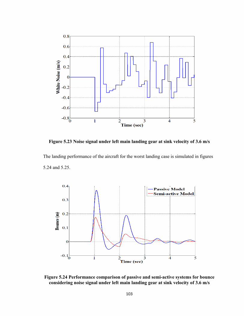
103
Figure 5.23 Noise signal under left main landing gear at sink velocity of 3.6 m/s
The landing performance of the aircraft for the worst landing case is simulated in figures
5.24 and 5.25.
Figure 5.24 Performance comparison of passive and semi-active systems for bounce considering noise signal under left main landing gear at sink velocity of 3.6 m/s
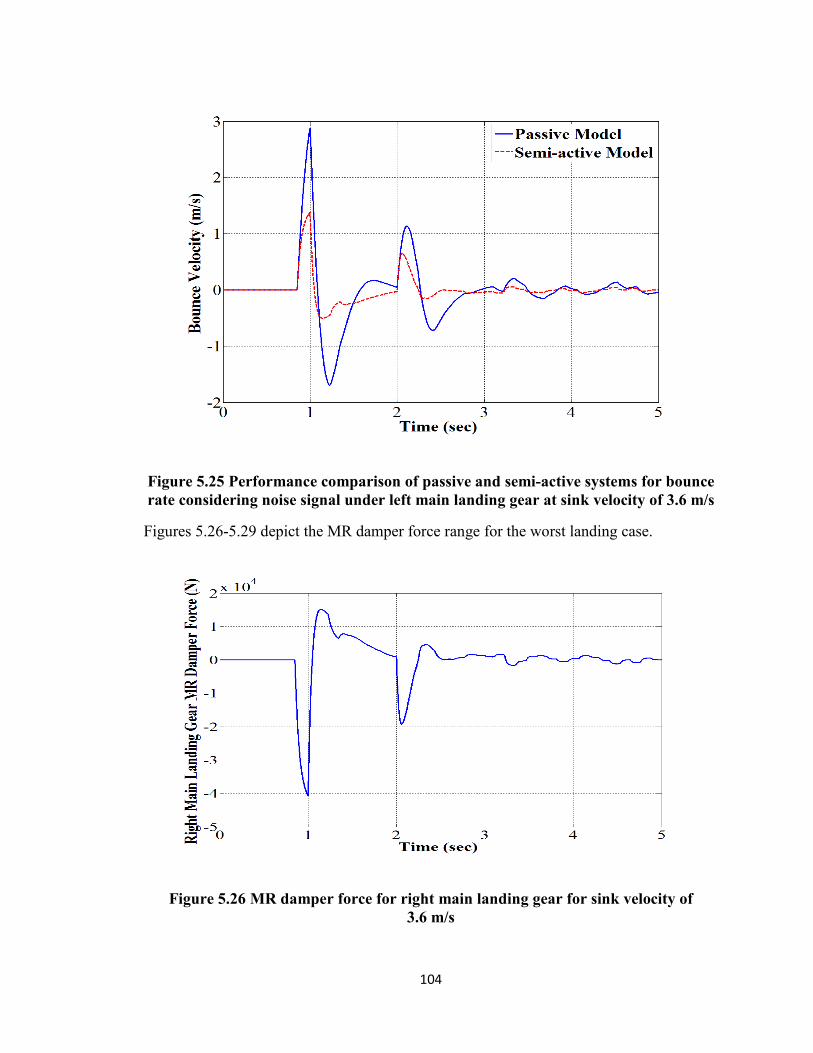
104
Figure 5.25 Performance comparison of passive and semi-active systems for bounce rate considering noise signal under left main landing gear at sink velocity of 3.6 m/s
Figures 5.26-5.29 depict the MR damper force range for the worst landing case.
Figure 5.26 MR damper force for right main landing gear for sink velocity of 3.6 m/s
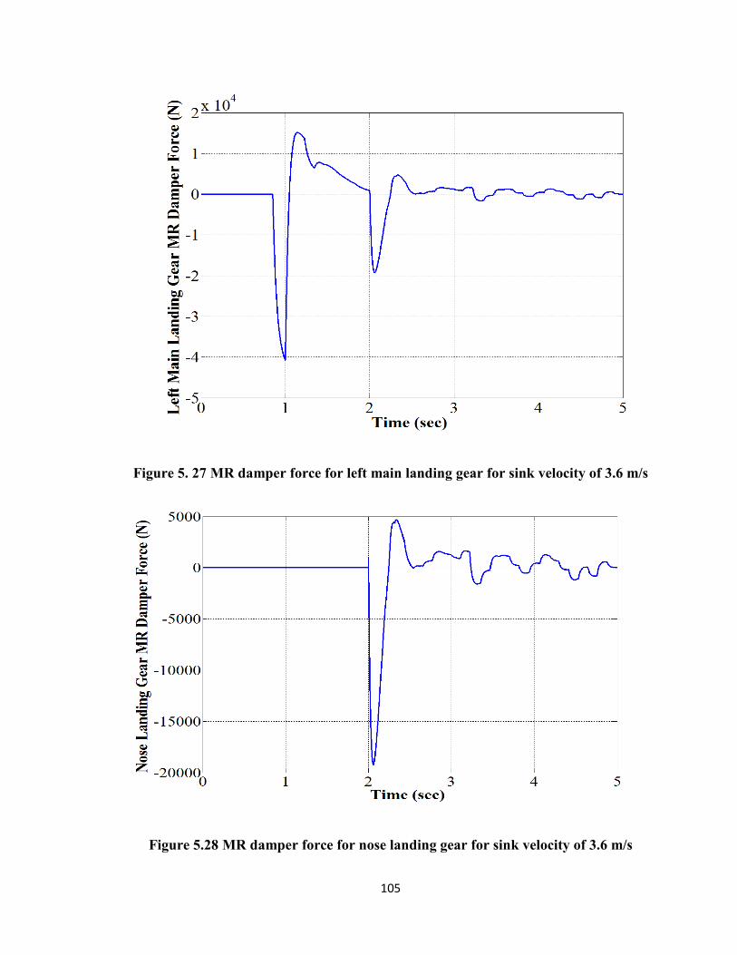
105
Figure 5. 27 MR damper force for left main landing gear for sink velocity of 3.6 m/s
Figure 5.28 MR damper force for nose landing gear for sink velocity of 3.6 m/s
106
The bounce and the bounce rate responses depicted in the figures 5.24 and 5.25,
respectively, clearly indicate the effectiveness of the designed semi-active system for the
adverse landing conditions. The amplitude of the peaks increased as the aircraft landed on
a rough airstrip with comparatively higher landing velocity. However, for the worst case
landing also, the H∞ controller could damp out the vibrations getting transmitted to the
fuselage effectively. It can be observed from figures 5.26-5.28 that the required MR
damper forces have increased compared to the previous cases of landing. The MR
dampers embedded in two main landing gears and a nose gears are required to generate a
force of approximately 40 kN and 20 kN respectively, to supress the fuselage vibrations
during the possible worst landing case described above. Moreover, the aircraft takes
considerably less time to stabilize after the initial impact.
It can be interpreted from the results that the designed semi-active suspension
with the H∞ controller is adaptable to the uncertainties during landing. The system can
effectively reduce the fuselage vibrations both for the normal landing as well as the worst
lading case. In real landing scenarios, if the aircraft exceeds its sink speed limit and lands
on a rough airstrip, there is a possibility of accident during landing. From the results it
can be observed that the designed system is able to supress the fuselage vibrations
significantly not only for higher sink velocities but also in case of the other disturbance
occurring during landing like runway roughness.
107
5.4 Summary
In this chapter, the performance analysis of the designed semi-active MR landing gear
system is carried out by taking into consideration different landing scenarios. The
simulated results prove that the use of robust H∞ controller can significantly reduce the
overshoot of the bounce and bounce rate responses which are related to the ride comfort
of the aircraft after the initial landing impact. However, it is possible to carry out the
LQR design at more than one operating points and attempt gain scheduling to further
optimize the performance. Using robust control approach, the overshoot and settling time
are significantly reduced. The simulation results prove the ability of the control strategy
to generate required MR damper force for the initial landing scenario irrespective of the
external environment. The robust analysis shows that the H∞ controller is more efficient
than the LQR not only for the ideal landing but also for the worst landing case. The H∞
controller can accurately predict the required force corresponding to the MR damper
current. Therefore, it can be interpreted that the semi-active MR damper suspension
system using the H∞ approach is able to absorb the excessive fuselage vibrations
effectively during each landing. By considerably reducing the rate of bounce for the
realistic landing scenario, the passenger safety and comfort are improved during the
landing operation.
108
CHAPTER 6
CONCLUSIONS AND FUTURE RECOMMENDATIONS
6.1 Thesis Contributions
This study focuses on the development of the semi-active suspensions for the aircraft
landing gears implementing a robust H∞ control strategy and an optimal Linear Quadratic
Regulator (LQR) control strategy. The primary goal of designing an intelligent
suspension is to supress the excessive vibrations that are transferred to the aircraft
fuselage during the landing phase which is considered as the most critical operational
phase. This issue is directly related to the passenger safety and comfort. Therefore, the
goal is to make the aircraft landing as smooth and as comfortable as possible. It is evident
from the literature that the Magnetorheological dampers can form the basis for
developing intelligent suspension systems for aircraft. The unique ability of these
dampers to provide a variable damping effect at nominal currents makes them very
attractive for the suspension applications. These dampers can provide a rapid interface
between the mechanical systems and the electronic controls. Moreover, in case of failure,
they have the capability to act as passive damping devices. Because of their unique
characteristics, the MR dampers and their applications in engineering has been the focus
of many research studies.
To fulfil the objectives of this study, a simulation approach was presented and a 3
DOF aircraft model was developed which took into consideration the bounce, pitch and
roll motions of the aircraft during landing. The aircraft was assumed to be equipped with
a conventional tri-cycle landing gear system with one wheel per landing gear. An actual
109
landing scenario was simulated using MATLAB/SIMULINK by providing a specific sink
velocity and a time delay between the touchdown of the main wheels and the nose wheel.
A semi-active Magnetorheological suspension system was developed using a robust H∞
controller and an optimal LQR controller and the response of the aircraft was analyzed
for different sink velocities during landing. The performance of the two controllers was
compared for a particular landing scenario for the purpose of selecting the appropriate
control approach. Finally, the applicability of the developed semi-active suspension
system with the robust controller was tested by subjecting the landing aircraft to runway
input. Based on the mathematical and the simulation studies done on the developed
model, following are the important contributions of this study.
• Based on the available Spencer model, the analysis of the energy dissipation
characteristics of the MR damper is carried out. The energy dissipation patterns
for different input frequencies are analyzed and the mathematical equations for
linearizing the MR damper through simulation approach are presented. The
relationship between the dissipated energy and the current is depicted through
simulations. Similarly, the relationship between the equivalent damping
coefficient and the current is also established. The analysis of the energy
dissipation patterns of the MR damper and the graphically depicted relationships
with the applied inputs can give a better understanding of the behaviour of the
damper in order to effectively use it for the variable damping applications.
• A 3 DOF aircraft model is developed for the vibration analysis which takes into
consideration the bounce, pitch and roll motions of the aircraft. Most of the
aircraft models developed in the previous studies were based on the conventional
110
quarter car model which could take into account only the vertical vibrations.
However, the model developed in this study could be used to present the real
aircraft equipped with a tri-cycle landing gear system. The effects of the roll and
pitch motions on the vertical motion are also taken into consideration though
these motions are not analyzed in this study. Since most of today’s passenger
aircraft use a conventional tri-cycle landing gear system, this model can be used
for the simulation studies of the prototypes.
• The most important contribution is the simulation of the actual landing scenario
for the developed 3 DOF aircraft model. A switching technique is developed in
SIMULINK which enables the system to switch from a single degree of freedom
to three degrees of freedom system in order to simulate the sequential touching of
the two wheels of the main landing gears and the nose landing gear wheel during
landing. This approach can provide a good approximation of the real landing
scenarios in case of pilot inaccuracies and the other uncertainties.
111
6.2 Conclusions
The proposed study focused on the two important aspects; analyzing the behavior of the
Magnetorheological dampers using parametric dynamic modeling approach and
developing the semi-active MR landing gear suspension using the robust H∞ and the LQR
control strategies for reducing the fuselage vibrations. Based on the work done in this
study, the important conclusions can be summarized as follows:
• The Magnetorheological dampers can provide an effective solution for developing
the semi-active suspensions for the aircraft. Although a few applications of these
dampers have been reported in vehicle engineering field, aircraft landing gears
have not been equipped with such damper. MR fluids have the ability to make
rapid and reversible transitions in their rheological properties. This fact makes the
MR damper a powerful device for achieving the variable damping in suspension
systems with minimal power requirements.
• Parametric dynamic modeling approach for studying the non-linear hysteretic
characteristics of the MR dampers is a simple and robust modeling approach. The
parametric modeling approach facilitates the numerical analysis as well as the
simulation for studying the dynamic behavior of the MR dampers.
• It can be interpreted from the force-velocity characteristics that the MR dampers
operate in two distinct regions namely, the post-yield and the pre-yield region.
The force-velocity characteristics show hysteretic behavior which has to be
predicted accurately for implementing the control laws. Spencer dynamic model
can accurately depict the behavior of the MR damper by characterizing the post-
112
yield and the pre-yield hysteresis. The mathematical equations of Spencer model
are easy to understand and implement in the simulation.
• The energy dissipation results were also simulated using Spencer model. The
model could accurately predict the energy dissipation patterns of the MR damper
for varying input frequencies.
• The MR damper can be an effective actuation mechanism for developing the
semi-active suspension for the aircraft landing gears. The semi-active MR landing
gear was developed using the H∞ and the LQR control strategies. The simulated
results showed that the use of robust H∞ controller can significantly reduce the
overshoot of the bounce and bounce rate response which is related to the ride
comfort of the aircraft after the initial landing impact.
• Using robust control approach, the overshoot and settling time are significantly
reduced. The simulation results proved the ability of the control strategy to
generate the required MR damper force for the initial landing scenario
irrespective of the external environment. The robust analysis showed that the H∞
controller is more efficient than the LQR not only for the ideal landing but also
for the rough landing case considering the uncertainties like runway roughness.
The H∞ controller can accurately predict the required MR damper force based on
the bounce velocity. Therefore, a semi-active MR landing gear suspension system
using the H∞ approach is able to suppress the excessive fuselage vibrations
effectively during each landing scenario. By considerably reducing the rate of
bounce for the realistic landing scenario, the passenger safety and comfort are
improved during the landing operation.
113
6.3 Future Recommendations
The analyses done in the research provided a stimulus for further extending the
dimensions of knowledge in the field of the aircraft landing and the passenger safety
associated with it. The concept of development of smart dampers for the aircraft landing
gears is amongst the emerging research topics which, if implemented considering the
engineering constraints, can effectively reduce the impact loads during the landing phase.
The primary focus of all the research programs is to make human life pleasant,
comfortable and safe. Considering the human life as the utmost important factor can give
a tremendous impetus for making progress in this research field.
This field has wide open scope, and some recommendations are made for the
future studies. A few of them are summarized as follows.
• In this study, a 3 DOF aircraft model is developed for the vibration analysis. A
model considering the additional yaw DOF can be developed in order to consider
the shimmy motion occurring during landing. The application of the smart MR
damper for shimmy control is also recommended.
• Since the primary objective is to improve the ride comfort and passenger safety, it
is necessary to model the human body sitting inside an aircraft as a spring-mass-
damper system for analyzing the vibration transmissibility to the human body
through the fuselage. The human body of a pilot inside a cockpit can be modeled
for the transmissibility analysis as the safety of the pilot is extremely important.
This analysis can provide an actual idea of the passenger comfort during landing.
• The smaller capacity and light weight MR dampers can be used for the aircraft
seats to attenuate the vibrations during the landing impact. However, this
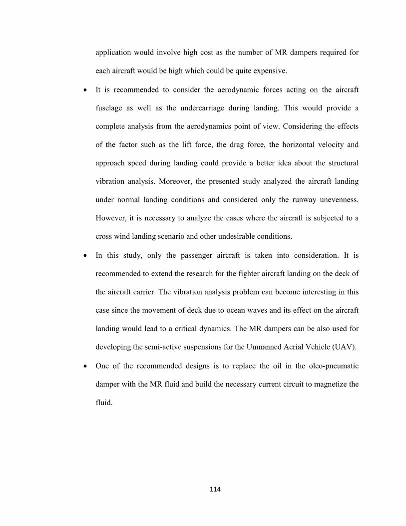
114
application would involve high cost as the number of MR dampers required for
each aircraft would be high which could be quite expensive.
• It is recommended to consider the aerodynamic forces acting on the aircraft
fuselage as well as the undercarriage during landing. This would provide a
complete analysis from the aerodynamics point of view. Considering the effects
of the factor such as the lift force, the drag force, the horizontal velocity and
approach speed during landing could provide a better idea about the structural
vibration analysis. Moreover, the presented study analyzed the aircraft landing
under normal landing conditions and considered only the runway unevenness.
However, it is necessary to analyze the cases where the aircraft is subjected to a
cross wind landing scenario and other undesirable conditions.
• In this study, only the passenger aircraft is taken into consideration. It is
recommended to extend the research for the fighter aircraft landing on the deck of
the aircraft carrier. The vibration analysis problem can become interesting in this
case since the movement of deck due to ocean waves and its effect on the aircraft
landing would lead to a critical dynamics. The MR dampers can be also used for
developing the semi-active suspensions for the Unmanned Aerial Vehicle (UAV).
• One of the recommended designs is to replace the oil in the oleo-pneumatic
damper with the MR fluid and build the necessary current circuit to magnetize the
fluid.
115
REFERENCES
[1] D. Howe, Aircraft loading and structural layout. London: Professional Engineering
Publishing, 2004.
[2] N. S. Currey, Aircraft landing gear design: Principles and practices. Washington
D.C.: American Institute of Aeronautics and Astronautics, Inc., 1988.
[3] Y. Xie et al., “Runway landing safety analysis: a case study of Atlanta Hartsfield
airport,” Proc. The 22nd IEEE Digital Avionics Systems Conference, vol. 1, pp. 1-12,
2003.
[4] H. Sheikhpour et al., “An approach on take-off and landing related aircraft accidents
involving new considerations,” International Conference on Traffic and
Transportation Engineering, Singapore, 2012, pp. 49-53.
[5] G. W. H. Van Es, “Running out of runway analysis of 35 years of landing overrun
accidents,” National Aerospace Laboratory NLR, Amsterdam, Rep. NLR-TP-2005-
498, 2005.
[6] F. Mirzatolooei and A. Bazzazi, “Analysis of orthopedic injuries in an airplane
landing disaster and a suggested mechanism of trauma,” European Journal of
Orthopaedic Surgery and Traumatology, vol. 23, pp. 257-262, 2013.
[7] H. Wentscher et al., “Fuselage vibration control using semi-active front gear,”
Advisory Group for Aerospace Research and Development North Atlantic Treaty
Organization (AGARD), Rep. R-800:5, 1996.
[8] A. Krauss, “The Design, qualification and maintenance of vibration-free landing
gear,” Daimler-Benz Aerospace AG, Munich, Rep. AGARD R-800, 1995.
116
[9] D. W. Young, “Aircraft landing gears-the past, present and future,” Proc. The
Institute of Mechanical Engineers, Part D: Journal of Automobile Engineering, vol.
200, pp. 75-92, 1986.
[10] D. C. Batterbee et al., “Magnetorheological landing gear: 1.a design methodology,”
Smart Materials and Structures, vol. 16, pp. 2429-2440, 2007.
[11] C. B. Asthana and R. B. Bhat, “Novel design of landing gear oleo strut damper
using fluid for aircraft and UAV’s,” Applied Mechanics and Materials, vol. 225, pp.
275-280, 2012.
[12] M. Khani, “MR damper for landing gear system,” MAsc thesis, Dept. Mechanical
and Industrial Engineering., Concordia University., Montreal, QC, Canada, 2010.
[13] W. Kruger et al., “Aircraft landing gear dynamics: simulation and control,” Vehicle
System Dynamics: International Journal of Vehicle Mechanics and Mobility, vol. 28,
pp. 119-158, 1997.
[14] H. H. Somm et al., “Adaptive landing gear for improved taxi performance,” Boeing
Aerospace Company, Seattle, Rep. AFFDL-TR-77-119, 1977.
[15] E. R. Wang, “Syntheses and analyses of semi-active control algorithms for a
Magnetorheological damper for vehicle suspensions,” Ph.D. dissertation, Dept.
Mechanical and Industrial Engineering., Concordia University., Montreal, QC,
Canada, 2005.
[16] D. L. Margolis, “A procedure for comparing passive, active and semi-active
approaches to vibration isolation,” Journal of the Franklin Institute, Vol. 315, pp.
225-238, 1983.
117
[17] H. Du et al., “Semi-active H∞ control of vehicle suspension with magneto-
rheological dampers,” Journal of Sound and Vibration, vol. 283, pp. 981-996, 2005.
[18] E. R. Wang et al., “Semi-active control of vehicle vibration with MR-dampers,”
Proc. 42nd IEEE Conference on Decision and Control, vol. 3, pp. 2270-2275, 2003.
[19] M. Zapateiro et al., “Semiactive control methodologies for suspension control with
magnetorheological dampers,” IEEE/ASME Trans. Mechatronics, vol. 17, pp. 370-
380, 2012.
[20] L. Hua-Lin et al., “Fuzzy PID control for landing gear based on magneto-
rheological (MR) damper,” International Conference on Apperceiving Computing
and Intelligence Analysis., Chengdu., 2009, pp. 22-25.
[21] D. H. Wang and W. H. Liao, “Magnetorheological fluid dampers: a review of
parametric modeling,” Smart Materials and Structures, vol. 20, pp. 1-34, 2011.
[22] J. D. Carlson, “Commercial Magnetorheological fluid device,” International
Journal of Modern Physics B, Vol. 10, pp. 2857-2865, 1996.
[23] M. R. Jolly et al., “Properties and applications of commercial magnetorheological
fluids,” Journal of Intelligent Material Systems and Structures, vol. 10, pp. 5-13,
1996.
[24] M. Aslam et al., “Review of magnetorheological (MR) fluids and its applications in
vibration control,” Journal of Marine Science and Application, Vol. 5, pp. 17-29,
2006.
[25] J. D. Carlson and J. L. Sproston, “Controllable fluids in 2000 status of ER and MR
fluid technology,” Proc. 7th International Conference on New Actuators., Bremen,
2000, pp. 126-130.
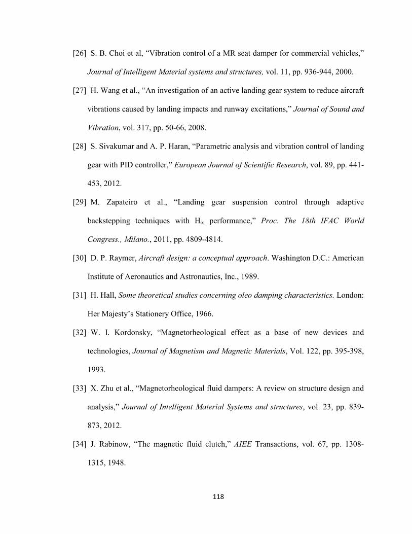
118
[26] S. B. Choi et al, “Vibration control of a MR seat damper for commercial vehicles,”
Journal of Intelligent Material systems and structures, vol. 11, pp. 936-944, 2000.
[27] H. Wang et al., “An investigation of an active landing gear system to reduce aircraft
vibrations caused by landing impacts and runway excitations,” Journal of Sound and
Vibration, vol. 317, pp. 50-66, 2008.
[28] S. Sivakumar and A. P. Haran, “Parametric analysis and vibration control of landing
gear with PID controller,” European Journal of Scientific Research, vol. 89, pp. 441-
453, 2012.
[29] M. Zapateiro et al., “Landing gear suspension control through adaptive
backstepping techniques with H∞ performance,” Proc. The 18th IFAC World
Congress., Milano., 2011, pp. 4809-4814.
[30] D. P. Raymer, Aircraft design: a conceptual approach. Washington D.C.: American
Institute of Aeronautics and Astronautics, Inc., 1989.
[31] H. Hall, Some theoretical studies concerning oleo damping characteristics. London:
Her Majesty’s Stationery Office, 1966.
[32] W. I. Kordonsky, “Magnetorheological effect as a base of new devices and
technologies, Journal of Magnetism and Magnetic Materials, Vol. 122, pp. 395-398,
1993.
[33] X. Zhu et al., “Magnetorheological fluid dampers: A review on structure design and
analysis,” Journal of Intelligent Material Systems and structures, vol. 23, pp. 839-
873, 2012.
[34] J. Rabinow, “The magnetic fluid clutch,” AIEE Transactions, vol. 67, pp. 1308-
1315, 1948.
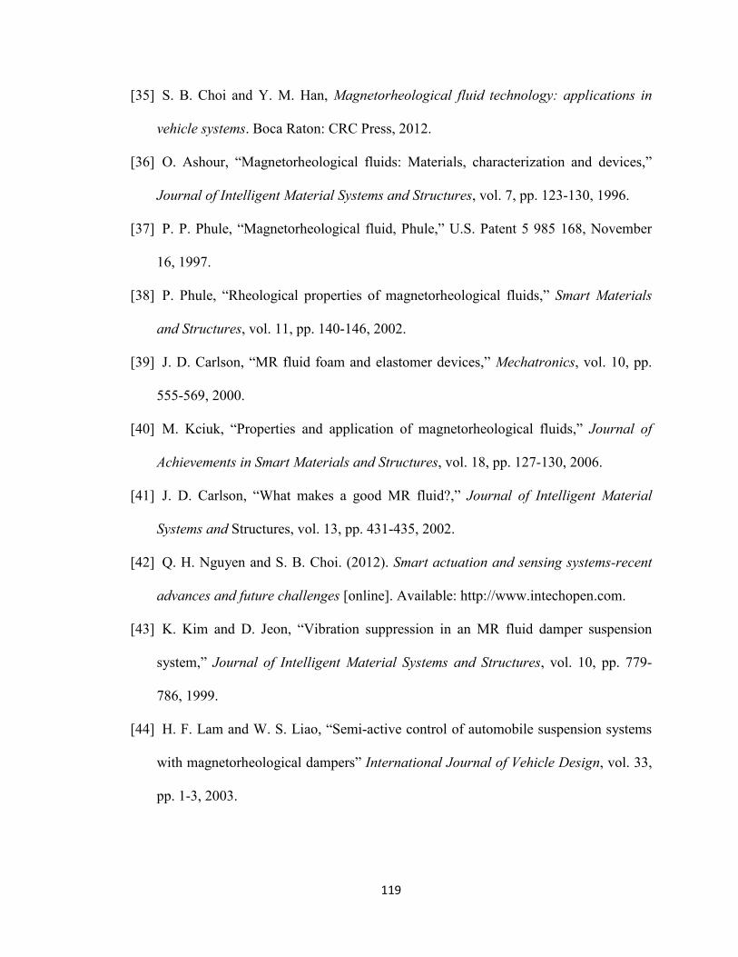
119
[35] S. B. Choi and Y. M. Han, Magnetorheological fluid technology: applications in
vehicle systems. Boca Raton: CRC Press, 2012.
[36] O. Ashour, “Magnetorheological fluids: Materials, characterization and devices,”
Journal of Intelligent Material Systems and Structures, vol. 7, pp. 123-130, 1996.
[37] P. P. Phule, “Magnetorheological fluid, Phule,” U.S. Patent 5 985 168, November
16, 1997.
[38] P. Phule, “Rheological properties of magnetorheological fluids,” Smart Materials
and Structures, vol. 11, pp. 140-146, 2002.
[39] J. D. Carlson, “MR fluid foam and elastomer devices,” Mechatronics, vol. 10, pp.
555-569, 2000.
[40] M. Kciuk, “Properties and application of magnetorheological fluids,” Journal of
Achievements in Smart Materials and Structures, vol. 18, pp. 127-130, 2006.
[41] J. D. Carlson, “What makes a good MR fluid?,” Journal of Intelligent Material
Systems and Structures, vol. 13, pp. 431-435, 2002.
[42] Q. H. Nguyen and S. B. Choi. (2012). Smart actuation and sensing systems-recent
advances and future challenges [online]. Available: http://www.intechopen.com.
[43] K. Kim and D. Jeon, “Vibration suppression in an MR fluid damper suspension
system,” Journal of Intelligent Material Systems and Structures, vol. 10, pp. 779-
786, 1999.
[44] H. F. Lam and W. S. Liao, “Semi-active control of automobile suspension systems
with magnetorheological dampers” International Journal of Vehicle Design, vol. 33,
pp. 1-3, 2003.
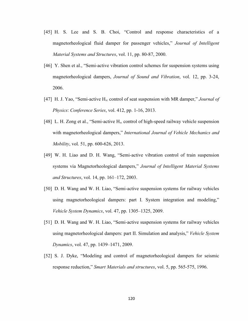
120
[45] H. S. Lee and S. B. Choi, “Control and response characteristics of a
magnetorheological fluid damper for passenger vehicles,” Journal of Intelligent
Material Systems and Structures, vol. 11, pp. 80-87, 2000.
[46] Y. Shen et al., “Semi-active vibration control schemes for suspension systems using
magnetorheological dampers, Journal of Sound and Vibration, vol. 12, pp. 3-24,
2006.
[47] H. J. Yao, “Semi-active H∞ control of seat suspension with MR damper,” Journal of
Physics: Conference Series, vol. 412, pp. 1-16, 2013.
[48] L. H. Zong et al., “Semi-active H∞ control of high-speed railway vehicle suspension
with magnetorheological dampers,” International Journal of Vehicle Mechanics and
Mobility, vol. 51, pp. 600-626, 2013.
[49] W. H. Liao and D. H. Wang, “Semi-active vibration control of train suspension
systems via Magnetorheological dampers,” Journal of Intelligent Material Systems
and Structures, vol. 14, pp. 161–172, 2003.
[50] D. H. Wang and W. H. Liao, “Semi-active suspension systems for railway vehicles
using magnetorheological dampers: part I. System integration and modeling,”
Vehicle System Dynamics, vol. 47, pp. 1305–1325, 2009.
[51] D. H. Wang and W. H. Liao, “Semi-active suspension systems for railway vehicles
using magnetorheological dampers: part II. Simulation and analysis,” Vehicle System
Dynamics, vol. 47, pp. 1439–1471, 2009.
[52] S. J. Dyke, “Modeling and control of magnetorheological dampers for seismic
response reduction,” Smart Materials and structures, vol. 5, pp. 565-575, 1996.
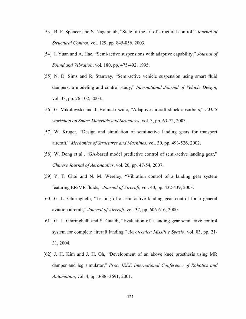
121
[53] B. F. Spencer and S. Nagarajaih, “State of the art of structural control,” Journal of
Structural Control, vol. 129, pp. 845-856, 2003.
[54] I. Yuan and A. Hac, “Semi-active suspensions with adaptive capability,” Journal of
Sound and Vibration, vol. 180, pp. 475-492, 1995.
[55] N. D. Sims and R. Stanway, “Semi-active vehicle suspension using smart fluid
dampers: a modeling and control study,” International Journal of Vehicle Design,
vol. 33, pp. 76-102, 2003.
[56] G. Mikulowski and J. Holnicki-szulc, “Adaptive aircraft shock absorbers,” AMAS
workshop on Smart Materials and Structures, vol. 3, pp. 63-72, 2003.
[57] W. Kruger, “Design and simulation of semi-active landing gears for transport
aircraft,” Mechanics of Structures and Machines, vol. 30, pp. 493-526, 2002.
[58] W. Dong et al., “GA-based model predictive control of semi-active landing gear,”
Chinese Journal of Aeronautics, vol. 20, pp. 47-54, 2007.
[59] Y. T. Choi and N. M. Wereley, “Vibration control of a landing gear system
featuring ER/MR fluids,” Journal of Aircraft, vol. 40, pp. 432-439, 2003.
[60] G. L. Ghiringhelli, “Testing of a semi-active landing gear control for a general
aviation aircraft,” Journal of Aircraft, vol. 37, pp. 606-616, 2000.
[61] G. L. Ghiringhelli and S. Gualdi, “Evaluation of a landing gear semiactive control
system for complete aircraft landing,” Aerotecnica Missili e Spazio, vol. 83, pp. 21-
31, 2004.
[62] J. H. Kim and J. H. Oh, “Development of an above knee prosthesis using MR
damper and leg simulator,” Proc. IEEE International Conference of Robotics and
Automation, vol. 4, pp. 3686-3691, 2001.
122
[63] H. Herr and A. Wilkenfeld, “User-adaptive control of a magnetorheological
prosthetic knee,” Industrial Robot: An International Journal, Vol. 30, pp. 42–55,
2003.
[64] W. H. Li, “Viscoelastic properties of MR fluids,” Smart Materials and Structure,
vol. 8, pp. 460-468, 1998.
[65] J. Wang and G. Meng, “Magnetorheological fluid devices: Principles,
characteristics and applications in mechanical engineering,” Proc. The Institution of
Mechanical Engineers, Part L: Journal of Materials Design and Applications, vol.
215, pp. 165-174, 2001.
[66] D. H. Wang and T. Wang, “Principle, design and modeling of an integrated relative
displacement self-sensing magnetorheological damper based on electromagnetic
induction,” Smart Materials and Structures, vol. 18, pp. 950-970, 2009.
[67] S. B. Choi et al., “A hysteresis model for the field-dependent damping force of a
Magnetorheological damper,’’ Journal of Sound and Vibration, vol. 245, pp. 375–
383, 2001.
[68] G. Jin et al., “Modeling MR-dampers: A nonlinear blackbox approach,” Proc. IEEE
American Control Conference, vol. 1, pp. 429–434, 2001.
[69] S. M. Savaresi et al., “Identification of semi-physical and black-box non-linear
models: the case of MR-dampers for vehicles control,” Automatica, vol. 41, pp. 113–
27, 2005.
[70] D. H. Wang and W. H. Liao, “Modeling and control of magnetorheological fluid
dampers using neural networks,” Smart Materials and Structures, vol. 14, pp. 111–
126, 2005.
123
[71] N. M. Werely et al., “Idealized hysteresis modeling of electrorheological and
magnetorheological dampers,” Journal of Intelligent Material Systems and
Structures, pp. 642-649, 1998.
[72] R. Stanway et al., “Application of electrorheological fluids in vibration control: A
Survey, ” Smart Materials and Structures, Vol. 5, pp. 464-482, 1996.
[73] E. R. Wang et al., “Modeling the hysteretic characteristics of a magnetorheological
fluid damper,” Proc. Institution of Mechanical Engineers, Part D: Journal of
Automobile Engineering, vol. 217, pp. 537-550, 2003.
[74] X. Q. Ma et al., “Modeling hysteretic characteristics of MR-fluid damper and model
validation,” Proc. 41st IEEE Conf. on Decision and Control, vol. 2, pp.1675–1680,
2002.
[75] X. Q. Ma, “Relative assessments of current dependent models for magneto-
rheological fluid dampers,” Proc. IEEE International Conference on Networking,
Sensing and Control., Ft. Lauderdale, 2006, pp. 510–515.
[76] B. F. Spencer Jr. et al., “Phenomenological model of a magnetorheological
damper,” Journal of Engineering Mechanics, vol. 123, pp. 230-238, 1997.
[77] A. Dominguez et al., “A new dynamic hysteresis model for magnetorheological
dampers,” Smart Materials and Structures, vol. 15, pp. 1179–1189, 2006.
[78] A. Dominguez et al., “Semi-active vibration control of adaptive structures using
magnetorheological dampers,” AIAA Journal, vol. 44, pp. 1563–1571, 2006.
[79] X. Q. Ma et al., “Development and relative assessments of models for
characterizing the current dependent hysteresis properties of magnetorheological
124
fluid dampers,” Journal of Intelligent Material Systems and Structures, Vol. 18, pp.
487–502, 2007.
[80] X. Q. MA, “Dynamic characterization of a Magnetorheological fluid damper and
synthesis of a semi-active suspension seat,” Ph.D. dissertation, Dept. Mechanical and
Industrial Engineering., Concordia University., Montreal, QC, Canada, 2005.
[81] F. Ikhouane and J. Rodelar, “On the hysteretic Bouc-wen model,” Nonlinear
Dynamics, vol. 42, pp. 63-78, 2005.
[82] W. H. Liao and C. Y. Lai, “Harmonic analysis of a magnetorheological damper for
vibration control,” Smart Materials and Structures, vol.11, pp.288–296, 2002.
[83] B. Sapinski, “Linearized characterization of a magnetorheological fluid damper,”
Mechanics, vol. 24, pp. 144-149, 2005.
[84] W. H. Li et al., “Testing and steady state modeling of a linear MR damper under
sinusoidal loading,” Smart Materials and Structures, vol. 9, pp. 95–102, 2000.
[85] L. Pang et al., “Analysis and testing of a linear stroke Magnetorheological damper,”
Proc. The AIAA/ASME/AHS Adaptive Structures Forum, vol. CP9803, pp. 2841-
2856, 1998.
[86] G. Z. Yao, “MR damper and its application for semi-active control of vehicle
suspension system,” Mechatronics, vol. 12, pp. 963-973, 2002.
[87] G. Yang, et al., “Large-scale MR fluid dampers: modeling and dynamic
performance considerations,” Engineering Structures, vol. 24, pp. 309-323, 2002.
[88] R. C. Dorf and R. H. Bishop, Modern control systems. New Jersey: Prentice Hall,
2008.
125
[89] A. A. Stoorvogel, The H∞ control problem: a state-space approach. New Jersey:
Prentice Hall, 1992.
[90] A. F. Jarhomi and A. Zabihollah, “Linear quadratic regulator and Fuzzy controller
application in full-car model of suspension system with magnetorheological shock
Absorber,” IEEE/ASME Conference on Mechatronics and Embedded Systems and
Applications (MESA), Qingdao, 2010, pp. 522-528.
[91] M. S. Kumar and S. Vijayarangan, “Design of LQR controller for active suspension
system,” Indian Journal of Engineering and Material Sciences, vol. 13, pp. 173-179,
2006.
[92] A. H. Shirdel et al., “Comparison of H∞ and optimized-LQR controller in active
suspension system,” in The Second International Conference on Computational
Intelligence, Modeling and Simulation., Bali, 2010, pp. 241-246.
[93] H. Y. Son et al., “A robust controller design for performance improvement of a
semi-active suspension systems,” Proc. The IEEE International Symposium on
Industrial Electronics, vol. 3, pp. 1458-1461, 2001.
[94] M. S. Fallah et al., “Robust model predictive control of shimmy vibration in aircraft
landing gears,” AIAA Journal of Aircraft, vol. 45, pp. 1872-1880, 2008.
[95] W. S. Levine, The controls handbook (volume 1). Mumbai: Jaico Publishing House,
1999.
[96] R. S. Burns, Advance controls engineering. Oxford: Butterworth Heinemann, 2001.
[97] J. C. Doyle et al., “State-space solutions to standard H2 and H∞ control problems,”
IEEE Trans.on Automatic Control, pp. 831-846, 1989.
126
[98] J. J. D’ Azzo and C. H. Houpis, Linear control system analysis and design:
Conventional and modern. New York: McGraw-Hill Book Company, 1981.
[99] A. F. Jahromi et al., “Ride control of passenger cars with semiactive suspension
system using a linear quadratic regulator and hybrid optimization algorithm,” Proc.
International Conference on Aerospace, Mechanical, Automotive and Materials
Engineering (ICAMAME 2012), vol. 67, pp. 896-902, 2012.
[100] D. H. Perry, Measurements of the moments of inertia of the Avro 707B aircraft.
London: Her Majesty’s Stationery Office, 1963.
[101] H. H. Tsang et al., “Simplified inverse dynamic models for MR fluid dampers,”
Engineering Structures, vol. 28, pp. 327-341, 2006.
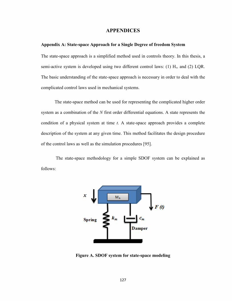
127
APPENDICES
Appendix A: State-space Approach for a Single Degree of freedom System
The state-space approach is a simplified method used in controls theory. In this thesis, a
semi-active system is developed using two different control laws: (1) H∞ and (2) LQR.
The basic understanding of the state-space approach is necessary in order to deal with the
complicated control laws used in mechanical systems.
The state-space method can be used for representing the complicated higher order
system as a combination of the N first order differential equations. A state represents the
condition of a physical system at time t. A state-space approach provides a complete
description of the system at any given time. This method facilitates the design procedure
of the control laws as well as the simulation procedures [95].
The state-space methodology for a simple SDOF system can be explained as
follows:
Figure A. SDOF system for state-space modeling
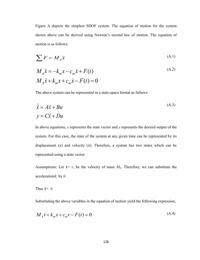
128
Figure A depicts the simplest SDOF system. The equation of motion for the system
shown above can be derived using Newton’s second law of motion. The equation of
motion is as follows:
(A.1)
(A.2)
The above system can be represented in a state-space format as follows:
(A.3)
In above equations, x represents the state vector and y represents the desired output of the
system. For this case, the state of the system at any given time can be represented by its
displacement (𝑥) and velocity (�̇�). Therefore, a system has two states which can be
represented using a state vector.
Assumptions: Let �̇�= v, be the velocity of mass MA. Therefore, we can substitute the
acceleration�̈�, by �̇�.
Thus �̈�= �̇�
Substituting the above variables in the equation of motion yield the following expression,
(A.4)
AF M x=∑
( )( ) 0
A m m
A m m
M x k x c x F tM x k x c x F t
= − − ++ + − =
x Ax Buy Cx Du= += +
( ) 0A m mM v k x c v F t+ + − =
129
The variable y represents the output of the system which is the displacement of the mass
MA for this case.
Therefore we have, 𝑦 = 𝑥
Finally, to determine the elements of the matrices in the state-space plant, following
equations can be used.
(A.5)
(A.6)
Referring to the state-space equation (A.3), the system in state-space can be represented
as follows:
(A.7)
In above equation, the matrices [A], [B] and [C] represent the system matrix, the input
matrix and the output matrix, respectively. The dimensions of these matrices can be
determined from the number of states, the inputs and outputs of the system.
Let N represents the number of states, R represents the number of inputs and P represents
the number of outputs of the system. The dimensions of the matrices can be defined as
follows.
x v=
1 ( )m m
A A A
k cv x v F tM M M
− −= + +
( )
( )
x xA BF t
v v
xy C DF t
v
= +
= +
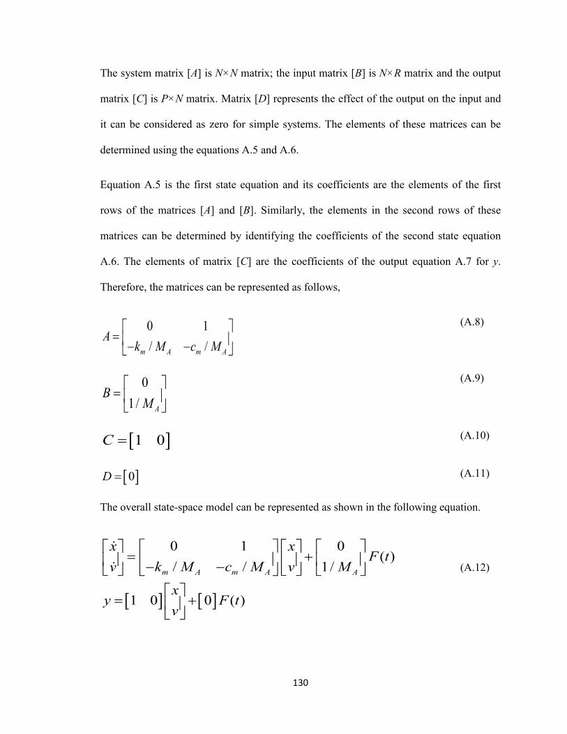
130
The system matrix [A] is N×N matrix; the input matrix [B] is N×R matrix and the output
matrix [C] is P×N matrix. Matrix [D] represents the effect of the output on the input and
it can be considered as zero for simple systems. The elements of these matrices can be
determined using the equations A.5 and A.6.
Equation A.5 is the first state equation and its coefficients are the elements of the first
rows of the matrices [A] and [B]. Similarly, the elements in the second rows of these
matrices can be determined by identifying the coefficients of the second state equation
A.6. The elements of matrix [C] are the coefficients of the output equation A.7 for y.
Therefore, the matrices can be represented as follows,
(A.8)
(A.9)
(A.10)
(A.11)
The overall state-space model can be represented as shown in the following equation.
(A.12)
0 1/ /m A m A
Ak M c M
= − −
01/ A
BM
=
[ ]1 0C =
[ ]0D =
[ ] [ ]
0 1 0( )
/ / 1/
1 0 0 ( )
m A m A A
x xF t
k M c M Mv v
xy F t
v
= + − −
= +
131
A state-space model can be represented in MATLAB using the inbuilt function and the
required response for a particular input signal can be achieved. A similar methodology is
adopted for a 3 DOF model used in this study which simplified the simulation
procedures.
132
Appendix B: Publications Revevant to Thesis work
In this section, the publications relevant to the study completed in this thesis are
presented. Following are the abstracts of the two conference papers relevant to this thesis.
1.
Optimally Adaptive Oleo Strut Damping for Aircraft and UAV Using MR Fluid
Authors: Ajinkya A. Gharapurkar, Dr. Chandra B. Asthana and Dr. Rama B. Bhat
1st Annual International Conference on Industrial and Systems Engineering, 24-27 June 2013, Athens, Greece
ABSTRACT
It would be most desirable to have the same oleo strut perform optimally during widely
different landing conditions of an aircraft and Unmanned Aerial Vehicle (UAV). These
landing conditions may impose different requirements such as controlling vertical
acceleration in a desired manner. As the atmospheric conditions change and the axial load
on the strut changes during compression, the ability to control the damping force as
function of time would be of great advantage. In this paper, it is shown that by using MR
fluid in the oleo strut, it is possible to achieve optimal damping performance in every
particular landing situation. Three different forces act along a conventional oleo strut
which are: that due to the compression/expansion of gas, that due to the passing of fluid
through the orifice and that due to the viscous force. The first is the spring force while the
second and the third are the damping forces. The second is proportional to the square of
compression/extension rate and the third is proportional to just the rate of
compression/extension. Incorporating a metering pin that can change the orifice diameter
in a prescribed fashion can change the damping force to some extent within limits. By
using MR fluid in a conventional oleo strut the damping force can be altered in a desired
133
manner. A simulation model for a SDOF aircraft system is developed and a landing
scenario at a particular sink velocity is simulated. The parameters controlling the
behavior of MR fluid damper are tuned to get the optimal performance during landing.
2.
Semi-Active Control of Aircraft Landing Gear System Using H-infinity Control Approach
Authors: Ajinkya A. Gharapurkar, Ali Fellah Jahromi, Dr. Rama B. Bhat and Dr.
Wen-Fang-Xie
The 2nd International Conference on Connected Vehicles & Expo (ICCVE 2013), 2013, Las Vegas, USA
ABSTARCT
The landing of an aircraft is one of the most critical operations because it directly affects
the passenger safety and comfort. During landing, the aircraft fuselage undergoes
excessive vibrations that cause the safety and the comfort problem and hence need to be
suppressed quickly. A semi-active control system of a landing gear suspension by using
Magnetorheological damper can solve the problem of excessive vibrations effectively. In
this paper, a switching technique is developed in the simulation of the landing procedure
which enables the system to switch from the single degree of freedom to three degrees of
freedom system in order to simulate the sequential touching of the two wheels of the
main landing gears and the nose landing gear wheels with the ground. A semi-active
Magnetorheological damper is developed using two different control strategies namely,
the Linear Quadratic Regulator and the H∞. Spencer model is used to predict the dynamic
behavior of the Magnetorheological damper. The results of the designed controllers are
compared to study the performance of the controllers in reducing the overshoot of the
bounce response as well as the bounce rate response. The simulation results validated the
134
improved performance of the robust controller compared to the optimal control strategy
when the aircraft is subjected to the disturbances during landing.
Appendix C: Calculation of current relative to MR damper force
The output of the MR damper is the MR damper force, while the input of the MR damper
model is a current signal function of time i (t). Therefore, a current signal corresponding
to the damping force should be calculated. The inverse dynamic model of the MR damper
using Spencer mathematical model is studied by Tsang et al. [101]. The mathematical
relation between the force and the current is represented in equation.
1 ( )
1 2
1( ) ln 1 3aj j b i t tF Fi t e j
d d− −∆
− = − + = −
where, Fa1-3 represents the actual force which can be measured during each iteration (Δt).
F1-3 presents the MR damper forces which are computed by the controller and defined by
equation derived by Spencer for the hysteretic damping force FD. The coefficients of the
MR damper model d1 and d2 can be calculated by using the curve fitting approach based
on the experimental results.


![arXiv:1407.0927v1 [cs.SE] 3 Jul 2014Landing-Gear Extended Landing-Gear Retracted Landing-Gear Box Landing Wheel Door Figure 1: Landing Gear System such as airport runways [11]. Three](https://static.fdocuments.in/doc/165x107/5e9397289f16a23cdf089611/arxiv14070927v1-csse-3-jul-2014-landing-gear-extended-landing-gear-retracted.jpg)