Robust Regression in Stata · Why is Low E ciency a Problem? An ine cient (yet unbiased) estimator...
44
Robust Regression in Stata Ben Jann University of Bern, [email protected] 10th German Stata Users Group meeting Berlin, June 1, 2012 Ben Jann (University of Bern) Robust Regression in Stata Berlin, 01.06.2012 1 / 34
Transcript of Robust Regression in Stata · Why is Low E ciency a Problem? An ine cient (yet unbiased) estimator...

Robust Regression in Stata
Ben Jann
University of Bern, [email protected]
10th German Stata Users Group meeting
Berlin, June 1, 2012
Ben Jann (University of Bern) Robust Regression in Stata Berlin, 01.06.2012 1 / 34

Outline
Introduction
Estimators for Robust Regression
Stata Implementation
Example
Ben Jann (University of Bern) Robust Regression in Stata Berlin, 01.06.2012 2 / 34

Introduction
Least-squares regression is a major workhorse in applied research.
It is mathematically convenient and has great statistical properties.
As is well known, the LS estimator is
I BUE (best unbiased estimator) under normally distributed errors
I BLUE (best linear unbiased estimator) under non-normal error
distributions
Furthermore, it is very robust in a technical sense (i.e. it is easily
computable under almost any circumstance).
Ben Jann (University of Bern) Robust Regression in Stata Berlin, 01.06.2012 3 / 34

Introduction
However, under non-normal errors better (i.e. more efficient)
(non-linear) estimators exist.
I For example, efficiency of the LS estimator can be poor if the error
distribution has fat tails (such as, e.g., the t-distribution with few
degrees of freedom).
In addition, the properties of the LS estimator only hold under the
assumption that the data comply to the suggested data generating
process.
I This may be violated, for example, if the data are “contaminated” by
a secondary process (e.g. coding errors).
Ben Jann (University of Bern) Robust Regression in Stata Berlin, 01.06.2012 4 / 34

Why is Low Efficiency a Problem?
An inefficient (yet unbiased) estimator gives the right answer on
average over many samples.
Most of the times, however, we only have one specific sample.
An inefficient estimator has a large variation from sample to sample.
This means that the estimator tends to be too sensitive to the
particularities of the given sample.
As a consequence, results from an inefficient estimator can be
grossly misleading in a specific sample.
Ben Jann (University of Bern) Robust Regression in Stata Berlin, 01.06.2012 5 / 34

Why is Low Efficiency a Problem?
Consider data from model
Y = β1 + β2X + e with β1 = β2 = 0 and e ∼ t(2)0
.1.2
.3.4
Density
-4 -2 0 2 4
t(2)normal
Ben Jann (University of Bern) Robust Regression in Stata Berlin, 01.06.2012 6 / 34

Why is Low Efficiency a Problem?
Consider data from model
Y = β1 + β2X + e with β1 = β2 = 0 and e ∼ t(2)
0.1
.2.3
.4Density
-4 -2 0 2 4
t(2)normal
2012-06-03
Robust Regression in Stata
Why is Low Efficiency a Problem?
. two (function y = normalden(x), range(-4 4) lw(*2) lp(dash)) ///¿ (function y = tden(2,x) , range(-4 4) lw(*2)) ///¿ , ytitle(Density) xtitle(””) ysize(3) ///¿ legend(order(2 ”t(2)” 1 ”normal”) col(1) ring(0) pos(11))

Why is Low Efficiency a Problem?
-50
510
1520
Y
0 2 4 6 8 10X
LS M MM
Sample 1
-8-6
-4-2
02
Y
0 2 4 6 8 10X
LS M MM
Sample 2
Ben Jann (University of Bern) Robust Regression in Stata Berlin, 01.06.2012 7 / 34

Why is Low Efficiency a Problem?
-50
510
1520
Y
0 2 4 6 8 10X
LS M MM
Sample 1
-8-6
-4-2
02
Y
0 2 4 6 8 10X
LS M MM
Sample 2
2012-06-03
Robust Regression in Stata
Why is Low Efficiency a Problem?
. drop ˙all
. set obs 31obs was 0, now 31
. generate x = (˙n-1)/3
. forvalues i = 1/2 –2. local seed: word `i´ of 669 7763. set seed `seed´4. generate y = 0 + 0 * x + rt(2)5. quietly robreg m y x6. predict m7. quietly robreg mm y x8. predict mm9. two (scatter y x, msymbol(Oh) mcolor(*.8)) ///
¿ (lfit y x, lwidth(*2)) ///¿ (line m mm x, lwidth(*2 *2) lpattern(shortdash dash)) ///¿ , nodraw name(g`i´, replace) ytitle(”Y”) xtitle(”X”) ///¿ title(Sample `i´) scale(*1.1) ///¿ legend(order(2 ”LS” 3 ”M” 4 ”MM”) rows(1))10. drop y m mm11. ˝
. graph combine g1 g2

Why is Contamination a Problem?
Assume that the data are generated by two processes.
I A main process we are interested in.
I A secondary process that “contaminates” the data.
The LS estimator will then give an answer that is an “average” of
both processes.
Such results can be meaningless because they represent neither the
main process nor the secondary process (i.e. the LS results are
biased estimates for both processes).
It might be sensible to have an estimator that only picks up the main
processes. The secondary process can then be identified as deviation
from the first (by looking at the residuals).
Ben Jann (University of Bern) Robust Regression in Stata Berlin, 01.06.2012 8 / 34

Hertzsprung-Russell Diagram of Star Cluster CYG OB1
3.5
4.0
4.5
5.0
5.5
6.0
6.5
Log
light
inte
nsity
3.43.63.84.04.24.44.6Log temperature
LS M MM
(Exa
mp
lefr
om
Ro
uss
ee
uw
an
dL
ero
y1
98
7:2
7-2
8)
Ben Jann (University of Bern) Robust Regression in Stata Berlin, 01.06.2012 9 / 34

Hertzsprung-Russell Diagram of Star Cluster CYG OB1
3.5
4.0
4.5
5.0
5.5
6.0
6.5
Log
light
inte
nsity
3.43.63.84.04.24.44.6Log temperature
LS M MM
(Exa
mp
lefr
om
Ro
uss
ee
uw
an
dL
ero
y1
98
7:2
7-2
8)
2012-06-03
Robust Regression in Stata
Hertzsprung-Russell Diagram of Star Cluster CYG OB1
. use starsCYG, clear
. quietly robreg m log˙light log˙Te
. predict m
. quietly robreg mm log˙light log˙Te
. predict mm
. two (scatter log˙light log˙Te, msymbol(Oh) mcolor(*.8)) ///¿ (lfit log˙light log˙Te, lwidth(*2)) ///¿ (line m log˙Te, sort lwidth(*2) lpattern(shortdash)) ///¿ (line mm log˙Te if log˙Te¿3.5, sort lwidth(*2) lpattern(dash)) ///¿ , xscale(reverse) xlabel(3.4(0.2)4.7, format(%9.1f)) ///¿ xtitle(”Log temperature”) ylabel(3.5(0.5)6.5, format(%9.1f)) ///¿ ytitle(”Log light intensity”) ///¿ legen(order(2 ”LS” 3 ”M” 4 ”MM”) rows(1) ring(0) pos(12))

Efficiency of Robust Regression
Efficiency under non-normal errors
I A robust estimator should be efficient if the the errors do not follow a
normal distribution.
Relative efficiency
I In general, robust estimators should be relatively efficient for a wide
range of error distributions (including the normal distribution).
I For a given error distribution, the “relative efficiency” of a robust
estimator can be determined as follows:
RE =variance of the maximum-likelihood estimator
variance of the robust estimator
I Interpretation: Fraction of sample with which the ML estimator is still
as efficient as the robust estimator.
Gaussian efficiency
I Efficiency of a robust estimator under normal errors (compared to the
LS estimator, which is equal to the ML estimator in this case).
Ben Jann (University of Bern) Robust Regression in Stata Berlin, 01.06.2012 10 / 34

Breakdown Point of Robust Regression
Robust estimators should be resistant to a certain degree of data
contamination.
Consider a mixture distribution
Fε = (1− ε)Fθ + εG
where Fθ is the main distribution we are interested in and G is a
secondary distribution that contaminates the data.
The breakdown point ε∗ of an estimator θ̂(Fε) is the largest value
for ε, for which θ̂(Fε) as a function of G is bounded.
I This is the maximum fraction of contamination that is allowed before
θ̂ can take on any value depending on G .
The LS estimator has a breakdown point of zero (as do many of the
fist generation robust regression estimators).
Ben Jann (University of Bern) Robust Regression in Stata Berlin, 01.06.2012 11 / 34

First Generation Robust Regression Estimators
A number of robust regression estimators have been developed as
generalizations of robust estimators of location.
In the regression context, however, these estimators have a low
breakdown point if the design matrix X is not fixed.
The best known first-generation estimator is the so called
M-estimator by Huber (1973).
An extension are so called GM- or bounded influence estimators
that, however, do not really solve the low breakdown point problem.
Ben Jann (University of Bern) Robust Regression in Stata Berlin, 01.06.2012 12 / 34

First Generation Robust Regression Estimators
The M-estimator is defined as
β̂M = arg minβ̂
n∑i=1
ρ
(Yi − XTi β̂
σ
)
where ρ is a suitable “objective function”.
Assuming σ to be known, the M-estimate is found by solving
n∑i=1
ψ
(Yi − XTi β̂
σ
)Xi = 0
where ψ is the first derivative of ρ.
Ben Jann (University of Bern) Robust Regression in Stata Berlin, 01.06.2012 13 / 34

First Generation Robust Regression Estimators
Different choices for ρ lead to different variants of M-estimators.
For example, setting ρ(z) = 12z
2 we get the LS estimator. This
illustrates that LS is a special case of the M-estimator.
ρ and ψ of the LS estimator look as follows:
01
23
45
!(z)
-3 -2 -1 0 1 2 3z
-4-2
02
4"(z)
-3 -2 -1 0 1 2 3z
Ben Jann (University of Bern) Robust Regression in Stata Berlin, 01.06.2012 14 / 34

First Generation Robust Regression Estimators
Different choices for ρ lead to different variants of M-estimators.
For example, setting ρ(z) = 12z
2 we get the LS estimator. This
illustrates that LS is a special case of the M-estimator.
ρ and ψ of the LS estimator look as follows:
01
23
45
!(z)
-3 -2 -1 0 1 2 3z
-4-2
02
4"(z)
-3 -2 -1 0 1 2 3z
2012-06-03
Robust Regression in Stata
First Generation Robust Regression Estimators
. two function y = .5*xˆ2, range(-3 3) xlabel(-3(1)3) ///¿ ytitle(”–&rho˝(z)”) xtitle(z) nodraw name(rho, replace)
. two function y = x, range(-3 3) xlabel(-3(1)3) yline(0, lp(dash)) ///¿ ytitle(”–&psi˝(z)”) xtitle(z) nodraw name(psi, replace)
. graph combine rho psi, ysize(2.5) scale(*2)

First Generation Robust Regression Estimators
To get an M-estimator that is more robust to outliers than LS we
have to define ρ so that it grows slower than the ρ of LS.
In particular, it seems reasonable to chose ρ such that ψ is bounded
(ψ is roughly equivalent to the influence of a data point).
A possible choice is to set ρ(z) = |z |. This leads to the median
regression (a.k.a. L1-estimator, LAV, LAD).
01
23
!(z)
-3 -2 -1 0 1 2 3z
-1-.5
0.5
1"(z)
-3 -2 -1 0 1 2 3z
Ben Jann (University of Bern) Robust Regression in Stata Berlin, 01.06.2012 15 / 34

First Generation Robust Regression Estimators
To get an M-estimator that is more robust to outliers than LS we
have to define ρ so that it grows slower than the ρ of LS.
In particular, it seems reasonable to chose ρ such that ψ is bounded
(ψ is roughly equivalent to the influence of a data point).
A possible choice is to set ρ(z) = |z |. This leads to the median
regression (a.k.a. L1-estimator, LAV, LAD).
01
23
!(z)
-3 -2 -1 0 1 2 3z
-1-.5
0.5
1"(z)
-3 -2 -1 0 1 2 3z
2012-06-03
Robust Regression in Stata
First Generation Robust Regression Estimators
. two function y = abs(x), range(-3 3) xlabel(-3(1)3) ///¿ ytitle(”–&rho˝(z)”) xtitle(z) nodraw name(rho, replace)
. two function y = sign(x), range(-3 3) xlabel(-3(1)3) yline(0, lp(dash)) ///¿ ytitle(”–&psi˝(z)”) xtitle(z) nodraw name(psi, replace)
. graph combine rho psi, ysize(2.5) scale(*2)

First Generation Robust Regression Estimators
Unfortunately, the LAV-estimator has low gaussian efficiency
(63.7%).
This lead Huber (1964) to define an objective function that
combines the good efficiency of LS and the robustness of LAV.
Huber’s ρ and ψ are given as:
ρH(z) =
{12z
2 if |z | ≤ kk |z | − 1
2k2 if |z | > k
and ψH(z) =
k if z > k
z if |z | ≤ k−k if z < −k
Parameter k determines the gaussian efficiency of the estimator. For
example, for k = 1.35 gaussian efficiency is 95%.
I approaches LS if k →∞I approaches LAV if k → 0
Ben Jann (University of Bern) Robust Regression in Stata Berlin, 01.06.2012 16 / 34

First Generation Robust Regression Estimators
01
23
!(z)
-3 -2 -1 0 1 2 3z
-2-1
01
2"(z)
-3 -2 -1 0 1 2 3z
Ben Jann (University of Bern) Robust Regression in Stata Berlin, 01.06.2012 17 / 34

First Generation Robust Regression Estimators
01
23
!(z)
-3 -2 -1 0 1 2 3z
-2-1
01
2"(z)
-3 -2 -1 0 1 2 3z
2012-06-03
Robust Regression in Stata
First Generation Robust Regression Estimators
. local k 1.345
. two function y = cond(abs(x)¡=`k´ , .5*xˆ2 , `k´*abs(x) - 0.5*`k´ˆ2), ///¿ range(-3 3) xlabel(-3(1)3) ///¿ ytitle(”–&rho˝(z)”) xtitle(z) nodraw name(rho, replace)
. two function y = cond(abs(x)¡=`k´ , x, sign(x)*`k´), ///¿ range(-3 3) xlabel(-3(1)3) yline(0, lp(dash)) ///¿ ytitle(”–&psi˝(z)”) xtitle(z) nodraw name(psi, replace)
. graph combine rho psi, ysize(2.5) scale(*2)
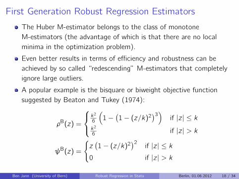
First Generation Robust Regression Estimators
The Huber M-estimator belongs to the class of monotone
M-estimators (the advantage of which is that there are no local
minima in the optimization problem).
Even better results in terms of efficiency and robustness can be
achieved by so called “redescending” M-estimators that completely
ignore large outliers.
A popular example is the bisquare or biweight objective function
suggested by Beaton and Tukey (1974):
ρB(z) =
k2
6
(1−
(1− (z/k)2
)3)
if |z | ≤ kk2
6 if |z | > k
ψB(z) =
{z(
1− (z/k)2)2
if |z | ≤ k0 if |z | > k
Ben Jann (University of Bern) Robust Regression in Stata Berlin, 01.06.2012 18 / 34

First Generation Robust Regression Estimators
0.2
.4.6
.81
!(z)
-3 -2 -1 0 1 2 3z
-1-.5
0.5
1"(z)
-3 -2 -1 0 1 2 3z
Again, k determines gaussian efficiency (e.g. 95% for k = 4.69).
Optimization has local minima. Therefore, the bisquare M is often
used with starting values from Huber M (as in Stata’s rreg).
Ben Jann (University of Bern) Robust Regression in Stata Berlin, 01.06.2012 19 / 34

First Generation Robust Regression Estimators
0.2
.4.6
.81
!(z)
-3 -2 -1 0 1 2 3z
-1-.5
0.5
1"(z)
-3 -2 -1 0 1 2 3z
Again, k determines gaussian efficiency (e.g. 95% for k = 4.69).
Optimization has local minima. Therefore, the bisquare M is often
used with starting values from Huber M (as in Stata’s rreg).
2012-06-03
Robust Regression in Stata
First Generation Robust Regression Estimators
. local k 2.5
. two fun y = cond(abs(x)¡=`k´, `k´ˆ2/6*(1-(1- (x/`k´)ˆ2)ˆ3), `k´ˆ2/6), ///¿ range(-3 3) xlabel(-3(1)3) ///¿ ytitle(”–&rho˝(z)”) xtitle(z) nodraw name(rho, replace)
. two function y = cond(abs(x)¡=`k´, x*(1- (x/`k´)ˆ2)ˆ2, 0), ///¿ range(-3 3) xlabel(-3(1)3) yline(0, lp(dash)) ///¿ ytitle(”–&psi˝(z)”) xtitle(z) nodraw name(psi, replace)
. graph combine rho psi, ysize(2.5) scale(*2)

First Generation Robust Regression Estimators
Computation of M-estimators
I M-estimators can be computed using an IRWLS algorithm (iteratively
reweighted least squares).
I The procedure iterates between computing weights from given
parameters and computing parameters from given weights until
convergence.
I The error variance is computed from the residuals using some robust
estimator of scale such as the (normalized) median absolute deviation.
Breakdown point of M-estimators
I M-estimators such as LAV, Huber, or bisquare are robust to
Y -outliers (as long as a robust estimate for σ is used).
I However, if X -outliers with high leverage are possible, then the
breakdown point drops to zero and not much is gained compared to
LS.
Ben Jann (University of Bern) Robust Regression in Stata Berlin, 01.06.2012 20 / 34

Second Generation Robust Regression Estimators
A number of robust regression estimators have been proposed to
tackle the problem of a low breakdown point in case of X outliers.
Early examples are LMS (least median of squares) and LTS (least
trimmed squares) (Rousseeuw and Leroy 1987).
LMS minimizes the median of the squared residuals
β̂LMS = arg minβ̂
MED(r(β̂)21, . . . , r(β̂)
2n)
and has a breakdown point of approximately 50%.
I It finds the “narrowest” band through the data that contains at least
50% of the data.
Ben Jann (University of Bern) Robust Regression in Stata Berlin, 01.06.2012 21 / 34

Second Generation Robust Regression Estimators
The LTS estimator follows a similar idea, but also takes into
account how the data are distributed within the 50% band.
It minimizes the variance of the 50% smallest residuals:
β̂LTS = arg minβ̂
h∑i=1
r(β̂)2(i) with h = bn/2c+ 1
where r(β̂)(i) are the ordered residuals.
LMS and LTS are attractive because of their high breakdown point
and their nice interpretation.
However, gaussian efficiency is terrible (0% and 7%, respectively).
Furthermore, estimation is tedious (jumpy objective function; lots of
local minima).
Ben Jann (University of Bern) Robust Regression in Stata Berlin, 01.06.2012 22 / 34

Second Generation Robust Regression Estimators
A better alternative is the so called S-estimator.
Similar to LS, the S-estimator minimizes the variance of the
residuals. However, it uses a robust measure for the variance.
It is defined as
β̂S = arg minβ̂
σ̂(r(β̂))
where σ̂(r) is an M-estimator of scale, found as the solution of
1
n − p
n∑i=1
ρ
(Yi − xTi β̂
σ̂
)= δ
with δ as a suitable constant to ensure consistency.
Ben Jann (University of Bern) Robust Regression in Stata Berlin, 01.06.2012 23 / 34
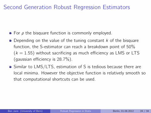
Second Generation Robust Regression Estimators
For ρ the bisquare function is commonly employed.
Depending on the value of the tuning constant k of the bisquare
function, the S-estimator can reach a breakdown point of 50%
(k = 1.55) without sacrificing as much efficiency as LMS or LTS
(gaussian efficiency is 28.7%).
Similar to LMS/LTS, estimation of S is tedious because there are
local minima. However the objective function is relatively smooth so
that computational shortcuts can be used.
Ben Jann (University of Bern) Robust Regression in Stata Berlin, 01.06.2012 24 / 34

Second Generation Robust Regression Estimators
The gaussian efficiency of the S-estimator is still unsatisfactory.
The problem is that in case of gaussian errors too much information
is thrown away.
High efficiency while preserving a high breakdown point is possible by
combining an S- and an M-estimator.
This is the so called MM-estimator. It works as follows:
1 Retrieve an initial estimate for β and an estimate for σ using the
S-estimator with a 50% breakdown point.2 Apply a redescending M-estimator (bisquare) using β̂S as starting
values (while keeping σ̂ fixed).
Ben Jann (University of Bern) Robust Regression in Stata Berlin, 01.06.2012 25 / 34

Second Generation Robust Regression Estimators
The higher the efficiency of the M-estimator in the second step, the
higher the maximum bias due to data contamination. An efficiency
of 85% is suggested as a good compromise (k = 3.44).
However, it can also be sensible to try different values to see how
the estimates change depending on k .
Ben Jann (University of Bern) Robust Regression in Stata Berlin, 01.06.2012 26 / 34

Second Generation Robust Regression Estimators
Brazil: Xingu
Brazil: Yanomamo
KenyaPapua New Guinea
9010
011
012
013
0M
edia
n sy
stol
ic b
lood
pre
ssur
e (m
m/H
g)
0 50 100 150 200 250Median urinary sodium (mmol/24h)
SMM-70MM-85
(In
ters
alt
Co
op
era
tive
Re
sea
rch
Gro
up
19
88
;F
ree
dm
an
/P
eti
tti
20
02
)
Ben Jann (University of Bern) Robust Regression in Stata Berlin, 01.06.2012 27 / 34

Second Generation Robust Regression Estimators
Brazil: Xingu
Brazil: Yanomamo
KenyaPapua New Guinea
9010
011
012
013
0M
edia
n sy
stol
ic b
lood
pre
ssur
e (m
m/H
g)
0 50 100 150 200 250Median urinary sodium (mmol/24h)
SMM-70MM-85
(In
ters
alt
Co
op
era
tive
Re
sea
rch
Gro
up
19
88
;F
ree
dm
an
/P
eti
tti
20
02
)
2012-06-03
Robust Regression in Stata
Second Generation Robust Regression Estimators
. use intersalt/intersalt, clear
. qui robreg s msbp mus
. predict s
. qui robreg mm msbp mus
. predict mm85
. qui robreg mm msbp mus, eff(70)
. predict mm70
. two (scatter msbp mus if mus¿60, msymbol(Oh) mcolor(*.8)) ///¿ (scatter msbp mus if mus¡60, msymbol(Oh) mlabel(centre)) ///¿ (line s mus, sort lwidth(*2)) ///¿ (line mm70 mus, sort lwidth(*2) lpattern(shortdash)) ///¿ (line mm85 mus, sort lwidth(*2) lpattern(dash)) ///¿ , ytitle(”`: var lab msbp´”) ///¿ legen(order(3 ”S” 4 ”MM-70” 5 ”MM-85”) cols(1) ring(0) pos(4))

Stata Implementation
Official Stata has the rreg command.
I It is essentially an M-estimator (Huber follwed by bisquare), but also
includes an initial step that removes high-leverage outliers (based on
Cook’s D). Nonetheless, it has a low breakdown point.
High breakdown estimators are provided by the robreg user
command.
I Supports MM, M, S, LMS, and LTS estimation.
I Provides robust standard errors for MM, M, and S estimation.
I Implements a fast algorithm for the S-estimator.
I Provides options to set efficiency and breakdown point.
I Available from SSC.
Ben Jann (University of Bern) Robust Regression in Stata Berlin, 01.06.2012 28 / 34

Stata Implementation
Ben Jann (University of Bern) Robust Regression in Stata Berlin, 01.06.2012 29 / 34

Example: Online Actions of Mobile Phones. robreg mm price rating startpr shipcost duration nbids minincr
Step 1: fitting S-estimate
enumerating 50 candidates (percent completed)0 20 40 60 80 100..................................................
refining 2 best candidates ... done
Step 2: fitting redescending M-estimate
iterating RWLS estimate ........................................... done
MM-Regression (85% efficiency) Number of obs = 99Subsamples = 50Breakdown point = .5M-estimate: k = 3.443686S-estimate: k = 1.547645Scale estimate = 32.408444Robust R2 (w) = .62236093Robust R2 (rho) = .22709915
Robustprice Coef. Std. Err. z P¿—z— [95% Conf. Interval]
rating .8862042 .274379 3.23 0.001 .3484312 1.423977startpr .0598183 .0618122 0.97 0.333 -.0613313 .1809679
shipcost -2.903518 1.039303 -2.79 0.005 -4.940515 -.8665216duration -1.86956 1.071629 -1.74 0.081 -3.969914 .2307951
nbids .6874916 .7237388 0.95 0.342 -.7310104 2.105994minincr 2.225189 .5995025 3.71 0.000 1.050185 3.400192˙cons 519.5566 23.51388 22.10 0.000 473.4702 565.6429
(Da
tafr
om
Die
km
an
ne
ta
l.2
00
9)
Ben Jann (University of Bern) Robust Regression in Stata Berlin, 01.06.2012 30 / 34

Example: Online Actions of Mobile Phones
ls rreg m lav mm85
rating 0.671** 0.830*** 0.767*** 0.861*** 0.886**(0.211) (0.190) (0.195) (0.233) (0.274)
startpr 0.0552 0.0830* 0.0715 0.0720 0.0598(0.0462) (0.0416) (0.0538) (0.0511) (0.0618)
shipcost -2.549* -2.939** -2.924** -3.154** -2.904**(1.030) (0.927) (1.044) (1.140) (1.039)
duration -0.200 -1.078 -0.723 -1.112 -1.870(1.264) (1.138) (1.217) (1.398) (1.072)
nbids 1.278 1.236* 1.190 0.644 0.687(0.677) (0.610) (0.867) (0.750) (0.724)
minincr 3.313*** 2.445*** 2.954** 2.747** 2.225***(0.772) (0.695) (1.060) (0.854) (0.600)
˙cons 505.8*** 505.4*** 505.7*** 513.7*** 519.6***(29.97) (26.98) (26.64) (33.16) (23.51)
N 99 99 99 99 99
Standard errors in parentheses* p¡0.05, ** p¡0.01, *** p¡0.001
Ben Jann (University of Bern) Robust Regression in Stata Berlin, 01.06.2012 31 / 34

Example: Online Actions of Mobile Phones
ls rreg m lav mm85
rating 0.671** 0.830*** 0.767*** 0.861*** 0.886**(0.211) (0.190) (0.195) (0.233) (0.274)
startpr 0.0552 0.0830* 0.0715 0.0720 0.0598(0.0462) (0.0416) (0.0538) (0.0511) (0.0618)
shipcost -2.549* -2.939** -2.924** -3.154** -2.904**(1.030) (0.927) (1.044) (1.140) (1.039)
duration -0.200 -1.078 -0.723 -1.112 -1.870(1.264) (1.138) (1.217) (1.398) (1.072)
nbids 1.278 1.236* 1.190 0.644 0.687(0.677) (0.610) (0.867) (0.750) (0.724)
minincr 3.313*** 2.445*** 2.954** 2.747** 2.225***(0.772) (0.695) (1.060) (0.854) (0.600)
˙cons 505.8*** 505.4*** 505.7*** 513.7*** 519.6***(29.97) (26.98) (26.64) (33.16) (23.51)
N 99 99 99 99 99
Standard errors in parentheses* p¡0.05, ** p¡0.01, *** p¡0.001
2012-06-03
Robust Regression in Stata
Example: Online Actions of Mobile Phones
. quietly reg price rating startpr shipcost duration nbids minincr
. eststo ls
. quietly rreg price rating startpr shipcost duration nbids minincr
. eststo rreg
. quietly robreg m price rating startpr shipcost duration nbids minincr
. eststo m
. quietly qreg price rating startpr shipcost duration nbids minincr
. eststo lav
. quietly robreg mm price rating startpr shipcost duration nbids minincr
. eststo mm85
. esttab ls rreg m lav mm85, compress se mti nonum
ls rreg m lav mm85
rating 0.671** 0.830*** 0.767*** 0.861*** 0.886**(0.211) (0.190) (0.195) (0.233) (0.274)
startpr 0.0552 0.0830* 0.0715 0.0720 0.0598(0.0462) (0.0416) (0.0538) (0.0511) (0.0618)
shipcost -2.549* -2.939** -2.924** -3.154** -2.904**(1.030) (0.927) (1.044) (1.140) (1.039)
duration -0.200 -1.078 -0.723 -1.112 -1.870(1.264) (1.138) (1.217) (1.398) (1.072)
nbids 1.278 1.236* 1.190 0.644 0.687(0.677) (0.610) (0.867) (0.750) (0.724)
minincr 3.313*** 2.445*** 2.954** 2.747** 2.225***(0.772) (0.695) (1.060) (0.854) (0.600)
˙cons 505.8*** 505.4*** 505.7*** 513.7*** 519.6***(29.97) (26.98) (26.64) (33.16) (23.51)
N 99 99 99 99 99
Standard errors in parentheses* p¡0.05, ** p¡0.01, *** p¡0.001

Example: Online Actions of Mobile Phones
-100
010
020
030
0Pa
rtial
Res
idua
l
0 10 20 30 40 50minincr
LS
-100
010
020
030
0Pa
rtial
Res
idua
l
0 10 20 30 40 50minincr
MM
Ben Jann (University of Bern) Robust Regression in Stata Berlin, 01.06.2012 32 / 34

Example: Online Actions of Mobile Phones
-100
010
020
030
0Pa
rtial
Res
idua
l
0 10 20 30 40 50minincr
LS
-100
010
020
030
0Pa
rtial
Res
idua
l
0 10 20 30 40 50minincr
MM
2012-06-03
Robust Regression in Stata
Example: Online Actions of Mobile Phones
. quietly reg price rating startpr shipcost duration nbids minincr
. predict ls˙cpr(option xb assumed; fitted values)(6 missing values generated)
. replace ls˙cpr = price - ls˙cpr + ˙b[minincr]*minincr(188 real changes made, 89 to missing)
. generate ls˙fit = ˙b[minincr]*minincr
. quietly robreg mm price rating startpr shipcost duration nbids minincr
. predict mm˙cpr(6 missing values generated)
. replace mm˙cpr = price - mm˙cpr + ˙b[minincr]*minincr(188 real changes made, 89 to missing)
. generate mm˙fit = ˙b[minincr]*minincr
. two (scatter ls˙cpr minincr if minincr¡40, ms(Oh) mc(*.8) jitter(1)) ///¿ (scatter ls˙cpr minincr if minincr¿40) ///¿ (line ls˙fit minincr, sort lwidth(*2)) ///¿ , title(LS) ytitle(Partial Residual) legend(off) ///¿ name(ls, replace) nodraw
. two (scatter mm˙cpr minincr if minincr¡40, ms(Oh) mc(*.8) jitter(1)) ///¿ (scatter mm˙cpr minincr if minincr¿40) ///¿ (line mm˙fit minincr, sort lwidth(*2)) ///¿ , title(MM) ytitle(Partial Residual) legend(off) ///¿ name(mm, replace) nodraw
. graph combine ls mm

Conclusions
High breakdown-point robust regression is now available in Stata.
Should we use it?
I Some people recommend using robust regression instead of classic
methods.
I However, I see it more as a diagnostic tool, yet less tedious then
classic regression diagnostics.
I A good advice is to use classic methods for most of the work, but
then check the models using robust regression.
I If there are differences, then go into details.
Outlook
I Robust GLM
I Robust fixed effects and instrumental variables regression
I Robust multivariate methods
I ...
Ben Jann (University of Bern) Robust Regression in Stata Berlin, 01.06.2012 33 / 34

References
Beaton, A.E., J.W. Tukey. 1974. The fitting of power series, meaning polynomials,
illustrated on band-spectroscopic data. Technometrics 16(2): 147-185.
Diekmann, A., B. Jann, D. Wyder. 2009. Trust and Reputation in Internet Auctions.
Pp. 139-165 in: K.S. Cook, C. Snijders, V. Buskens, C. Cheshire (ed.). eTrust. Forming
Relationships in the Online World. New York: Russell Sage Foundation.
Freedman, D.A., D.B. Petitti. 2002. Salt, blood pressure, and public policy.
International Journal of Epidemiology 31: 319-320.
Huber, P.J. 1964. Robust estimation of a location parameter. The Annals of
Mathematical Statistics, 35(1): 73-101.
Huber, P.J. 1973. Robust regression: Asymptotics, conjectures and monte carlo. The
Annals of Statistics 1(5): 799-821.
Intersalt Cooperative Research Group. 1988. Intersalt: an international study of
electrolyte excretion and blood pressure: results for 24 hour urinary sodium and
potassium excretion. British Medical Journal 297 (6644): 319-328.
Maronna, R.A., D.R. Martin, V.J. Yohai. 2006. Robust Statistics. Theory and Methods.
Chichester: Wiley.
Rousseeuw, P.J., A.M. Leroy. 1987. Robust Regression and Outlier Detection. New
York: Wiley.
Ben Jann (University of Bern) Robust Regression in Stata Berlin, 01.06.2012 34 / 34