1

Robust Real Time Pattern Matching usingBayesian Sequential Hypothesis Testing

Ofir Pele and Michael Werman

Abstract— This paper describes a method for robustreal time pattern matching. We first introduce a family ofimage distance measures, the “Image Hamming DistanceFamily”. Members of this family are robust to occlusion,small geometrical transforms, light changes and non-rigid deformations. We then present a novel Bayesianframework for sequential hypothesis testing on finite pop-ulations. Based on this framework, we design an optimalrejection/acceptance sampling algorithm. This algorithmquickly determines whether two images are similar withrespect to a member of the Image Hamming DistanceFamily. We also present a fast framework that designsa near-optimal sampling algorithm. Extensive experimen-tal results show that the sequential sampling algorithmperformance is excellent. Implemented on a Pentium 43GHz processor, detection of a pattern with 2197 pixels,in 640x480 pixel frames, where in each frame the patternrotated and was highly occluded, proceeds at only 0.022seconds per frame.

Index Terms— Pattern matching, template matching,pattern detection, image similarity measures, Hammingdistance, real time, sequential hypothesis testing, compos-ite hypothesis, image statistics, Bayesian statistics, finitepopulations

I. INTRODUCTION

M ANY applications in image processing andcomputer vision require finding a particular

pattern in an image,pattern matching. To be use-ful in practice, pattern matching methods must beautomatic, generic, fast and robust.

Pattern matching is typically performed by scan-ning the entire image, and evaluating a distancemeasure between the pattern and a local rectangularwindow. The method proposed in this paper is appli-cable to any pattern shape, even a non-contiguousone. We use the notion of “window” to cover allpossible shapes.

First, we introduce a family of image distancemeasures called the “Image Hamming Distance

O. Pele and M. Werman are with the The Hebrew University ofJerusalem e-mail:ofirpele,werman@cs.huji.ac.il

Manuscript received ; revised

Family”. A distance measure in this family is thenumber of non-similar corresponding features be-tween two images. Members of this family arerobust to occlusion, small geometrical transforms,light changes and non-rigid deformations.

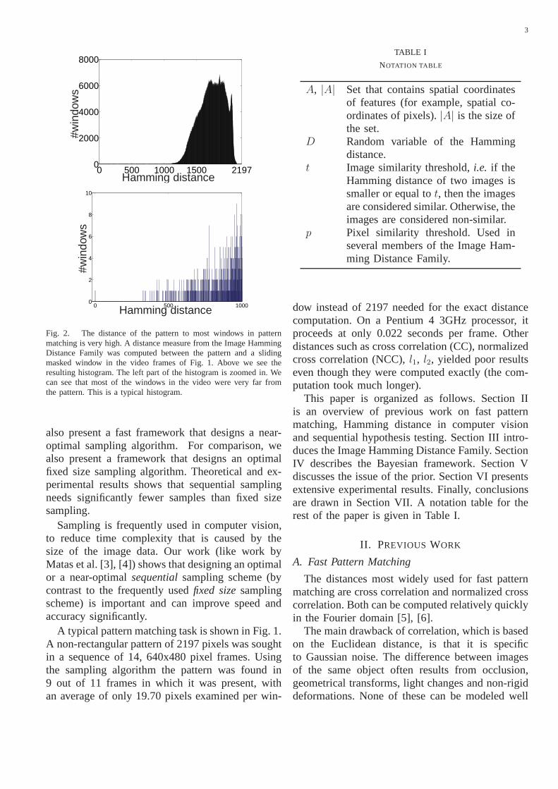
Second, we show how to quickly decide whethera window is similar to the pattern with respectto a member of the “Image Hamming DistanceFamily”. The trivial, but time consuming solution isto compute the exact distance between the patternand the window by going over all the correspondingfeatures (the simplest feature is a pixel). We presentan algorithm that samples corresponding featuresand accumulates the number of non-similar features.The speed of this algorithm is based on the factthat the distance between two non-similar imagesis usually very large whereas the distance betweentwo similar images is usually very small (see Fig.2). Therefore, for non-similar windows the sum willgrow extremely fast and we will be able to quicklydecide that they are non-similar. As the event ofsimilarity in pattern matching is so rare (see Fig.2), we can afford to pay the price of going over allthe corresponding features in similar windows. Notethat the algorithm does not attempt to estimate thedistances for non-similar windows. The algorithmonly decides that these windows, with a very highprobability (for example, 99.9%), are non-similar.The reduction in running time is due to the fact thatthis unnecessary information is not computed.

The idea of sequential sampling [1] or sequentialsampling a distance is not new [2]. The major con-tribution in our work is a novel efficient Bayesianframework for hypothesis testing on finite popula-tions. Given allowable bounds on the probabilityof error (false negatives and false positives) theframework designs a sampling algorithm that hasthe minimum expected running time. This is donein an offline phase for each pattern size. An onlinephase uses the sampling algorithm to quickly findpatterns. In order to reduce offline running time we

2

(a)

(b) (c) (d)

Fig. 1. Real time detection of a rotating and highly occludedpattern.(a) A non-rectangular pattern of 2197 pixels. Pixels not belonging to the mask are in black. (b) Three 640x480 pixel frames out of fourteenin which the pattern was sought. (c) The result. Most similarmasked windows are marked in white. (d) Zoom in of the occurrences of thepattern in the frames. Pixels not belonging to the mask are inblack.The SEQUENTIAL algorithm proceeds at only 0.022 seconds per frame. Offline running time - time spent on the parameterization of theSEQUENTIAL algorithm (with P-SPRT, see Section IV-D) was 0.067 seconds. Note that the distance is robust to out of plane rotations andocclusion. Using other distances such as CC, NCC,l2, l1 yielded poor results. In particular they all failed to find the pattern in the last frame.We emphasize that no motion consideration was taken into account in computation. The algorithm ran on all windows. Full size images areavailable at:http://www.cs.huji.ac.il/∼ofirpele/hs/all images.zip

3

0 500 1000 1500 21970

2000

4000

6000

8000

Hamming distance

#win

dow

s

0 500 10000

2

4

6

8

10

Hamming distance

#win

dow

s

Fig. 2. The distance of the pattern to most windows in patternmatching is very high. A distance measure from the Image HammingDistance Family was computed between the pattern and a slidingmasked window in the video frames of Fig. 1. Above we see theresulting histogram. The left part of the histogram is zoomed in. Wecan see that most of the windows in the video were very far fromthe pattern. This is a typical histogram.

also present a fast framework that designs a near-optimal sampling algorithm. For comparison, wealso present a framework that designs an optimalfixed size sampling algorithm. Theoretical and ex-perimental results shows that sequential samplingneeds significantly fewer samples than fixed sizesampling.

Sampling is frequently used in computer vision,to reduce time complexity that is caused by thesize of the image data. Our work (like work byMatas et al. [3], [4]) shows that designing an optimalor a near-optimalsequentialsampling scheme (bycontrast to the frequently usedfixed sizesamplingscheme) is important and can improve speed andaccuracy significantly.

A typical pattern matching task is shown in Fig. 1.A non-rectangular pattern of 2197 pixels was soughtin a sequence of 14, 640x480 pixel frames. Usingthe sampling algorithm the pattern was found in9 out of 11 frames in which it was present, withan average of only 19.70 pixels examined per win-

TABLE I

NOTATION TABLE

A, |A| Set that contains spatial coordinatesof features (for example, spatial co-ordinates of pixels).|A| is the size ofthe set.

D Random variable of the Hammingdistance.

t Image similarity threshold,i.e. if theHamming distance of two images issmaller or equal tot, then the imagesare considered similar. Otherwise, theimages are considered non-similar.

p Pixel similarity threshold. Used inseveral members of the Image Ham-ming Distance Family.

dow instead of 2197 needed for the exact distancecomputation. On a Pentium 4 3GHz processor, itproceeds at only 0.022 seconds per frame. Otherdistances such as cross correlation (CC), normalizedcross correlation (NCC),l1, l2, yielded poor resultseven though they were computed exactly (the com-putation took much longer).

This paper is organized as follows. Section IIis an overview of previous work on fast patternmatching, Hamming distance in computer visionand sequential hypothesis testing. Section III intro-duces the Image Hamming Distance Family. SectionIV describes the Bayesian framework. Section Vdiscusses the issue of the prior. Section VI presentsextensive experimental results. Finally, conclusionsare drawn in Section VII. A notation table for therest of the paper is given in Table I.

II. PREVIOUS WORK

A. Fast Pattern Matching

The distances most widely used for fast patternmatching are cross correlation and normalized crosscorrelation. Both can be computed relatively quicklyin the Fourier domain [5], [6].

The main drawback of correlation, which is basedon the Euclidean distance, is that it is specificto Gaussian noise. The difference between imagesof the same object often results from occlusion,geometrical transforms, light changes and non-rigiddeformations. None of these can be modeled well

4

with a Gaussian distribution. For a further discus-sion on Euclidean distance as a similarity measuresee [7]–[10]. Note that although the Hamming dis-tance is not specific to Gaussian noise as thel2norm, it is robust to Gaussian noise (see Fig. 3).Normalized cross correlation is invariant to additiveand multiplicative gray level changes. However, nat-ural light changes include different effects, such asshading, spectral reflectance, etc. In addition, whena correlation is computed in the transform domain,it can only be used with rectangular patterns andusually the images are padded so that their heightand width are dyadic.

Lucas and Kanade [11] employed the spatial in-tensity gradients of images to find a good match us-ing a Newton-Raphson type of iteration. The methodis based on Euclidean distance and it assumes thatthe two images are already in approximate registra-tion.

Local descriptors have been used recently forobject recognition [12]–[17]. The matching is doneby first extracting the descriptors and then matchingthem. Although fast, our approach is faster. Inaddition, there are cases where the local descriptorsapproach is not successful (see Fig. 7). If one knowsthat the object view does not change drastically,the invariance of the local descriptors can affectperformance and robustness [17]. In this work wedecided to concentrate on pixel values or simplerelation of pixels as features. Combining the se-quential sampling algorithm approach with the localdescriptors approach is an interesting extension ofthis work.

Recently there have been advances in the fieldof fast object detection using a cascade of rejectors[18]–[21]. Viola and Jones [20] demonstrated theadvantages of such an approach. They achieved realtime frontal face detection using a boosted cascadeof simple features. Avidan and Butman [21] showedthat instead of looking at all the pixels in the image,one can choose several representative pixels forfast rejection of non-face images. In this work wedo not deal with classification problems but ratherwith a pattern matching approach. Our approachdoes not include a learning phase. The learningphase makes classification techniques impracticalwhen many different patterns are sought or whenthe sought pattern is given online,e.g.in the case ofpatch-based texture synthesis [22], pattern matchingin motion estimation, etc.

Hel-Or and Hel-Or [23] used a rejection schemefor fast pattern matching with projection kernels.Their method is applicable to any norm distance,and was demonstrated on the Euclidean distance.They compute the Walsh-Hadamard basis projec-tions in a certain order. For the method to work fastthe first Walsh-Hadamard basis projections (accord-ing to the specific order) need to contain enoughinformation to discriminate most images. Ben-Artziet al. [24] proposed a faster projection schemecalled “Gray-Code Kernels”. Ben-Yehuda et al. [25]extended the Hel-Or pattern matching method tohandle non-rectangular patterns by decompositionof the pattern into several dyadic components.

Cha [26] uses functions that are lower boundsto the sum of absolute differences, and are fastto compute. They are designed to eliminate non-similar images fast. The first function he suggests isthe h-distance:

∑r−1k=0 |

∑kl=0(Gl(Im1) − Gl(Im2))|,

where Gl(Im) is the number of pixels with graylevel l in the intensity histogram of the image,Im,andr is the number of gray levels, usually 256. Thetime complexity is O(r). The second function hesuggests is the absolute value of difference betweensums of pixels:|

∑Im1(x, y) −

∑Im2(x, y)|. The

method is restricted to thel1 norm and assumes thatthese functions can reject most of the images fast.

One of the first rejection schemes was proposedby Barnea and Silverman [2]. They suggested theSequential Similarity Detection Algorithms - SSDA.The method accumulates the sum of absolute dif-ferences of the intensity values in both images andapplies a threshold criterion - if the accumulatedsum exceeds a threshold, which can increase withthe number of pixels, they stop and returnnon-similar. The order of the pixels is chosen randomly.After n iterations, the algorithm stops and returnssimilar. They suggested three heuristics for findingthe thresholds for thel1 norm. This method is veryefficient but has one main drawback. None of theheuristics for choosing the thresholds guarantees abound on the error rate. As a result the SSDA wassaid to be inaccurate [27]. Our work is a variation ofthe SSDA. We use a member of the Image HammingDistance Family instead of thel1 norm. We alsodesign a sampling scheme with proven error boundsand optimal running time. As the SSDA uses thel1norm, in each figure where thel1 norm yields poorresults (see Figs. 1, 4, 5 and 6) the SSDA also yieldspoor results.

5

(a)

(b) (c)

(a-zoom)

(d)

Fig. 3. Real time detection of a specific face in a noisy image of a crowd.(a) A rectangular pattern of 1089 pixels. (b) A noisy versionof the original 640x480 pixel image. The pattern that was taken from the originalimage was sought in this image. The noise is Gaussian with a mean of zero and a standard deviation of 25.5. (c) The result image. The singlesimilar masked window is marked in white. (d) The occurrenceof the pattern in the zoomed in image. TheSEQUENTIAL algorithm proceedsat only 0.019 seconds per frame. Offline running time - time spent on the parameterization of theSEQUENTIAL algorithm (with P-SPRT,see Section IV-D) was 0.018 seconds. Note that although the Hamming distance is not specific to Gaussian noise as thel2 norm, it is robustto Gaussian noise. The image is copyright by Ben Schumin and was downloaded from:http://en.wikipedia.org/wiki/Image:July 4 crowd at Vienna Metro station.jpg. Full size images are available at:http://www.cs.huji.ac.il/∼ofirpele/hs/all images.zip

Mascarenhas et al. [28], [29] used Wald’s Se-quential Probability Ratio Test (SPRT) [1] as thesampling scheme. Two models were suggested forthe random variable of the distance of the samplek. The first converts the images to binary and thenP (k) is binomially distributed. The second assumesthat the images are Gaussian distributed; henceP (k)is also Gaussian distributed. The likelihood ratio isdefined as:λ(k) = P (k|images are non-similar)

P (k|images are similar) . The SPRTsamples both images as long as:A < λ(k) < B.Whenλ(k) ≤ A the SPRT stops and returnssimilar.When λ(k) ≥ B the SPRT stops and returnsnon-similar. Let the bounds on the allowable error ratesbe P (false positive) = β, P (false negative) = α.Wald’s [1] approximation forA andB is A = β

1−α

, B = 1−β

α.

There are several problems with their method.Converting images to binary results in a loss ofinformation. In addition, gray levels are far frombeing Gaussian distributed [30]–[33]. Our methoddoes not assume any prior on the images. Mas-carenhas et al. assume that all similar images haveexactly the same pairwise small distance, whereasany two non-similar images have exactly the samelarge distance, an assumption that is faulty. Ourframework gets a prior on the distribution of imagedistances as input. The classical SPRT can go oninfinitely. There are ways to truncate it [34], butthey are not optimal. By contrast, we designed an

optimal rejection/acceptance sampling scheme witha restricted number of samples.

B. Hamming Distance in computer vision

Hamming Distance in computer vision [35]–[41]has usually been applied to a binary image, ordinar-ily a binary transform of a gray level image. Ionescuand Ralescu’s crisp version of the “fuzzy Hammingdistance” [39] is an exception, where a thresholdfunction is applied to decide whether two colors aresimilar.

A comprehensive review of local binary featuresof images and their usage for 2D Object detectionand recognition can be found in Amit’s book [35].Amit suggests using the Hough transform [42] tofind arrangements of the local binary features. InAppendix II we show how the Hough transformcan be used to compute the Hamming distance ofa pattern with all windows of an image. We alsoshow that the expected time complexity for eachwindow isO(|A|−E[D]), where|A| is the numberof pixels in the pattern’s set of pixels andD is therandom variable of the Hamming distance betweena random window and a random pattern. For thepattern matching in Fig. 1,E[D] = 1736.64, |A| =2197. Thus, the average work for each windowusing the Hough transform is460.36, much higherthan the19.70 needed using our approach, but muchless than comparing all the corresponding pixels.

6

Bookstein et al. [40] proposed the “GeneralizedHamming Distance” for object recognition on bi-nary images. The distance extends the Hammingconcept to give partial credit for near misses.They suggest a dynamic programming algorithmto compute it. The time complexity isO(|A| +∑

Im1∑

Im2), where|A| is the number of pixelsand

∑Im is the number of ones in the binary

image,Im. Our method is sub-linear. Another dis-advantage is that their method only copes with nearmisses in the horizontal direction. We suggest usingthe Local Deformationsmethod (see Section III) tohandle near misses in all directions.

C. Sequential Hypothesis Testing

Sequential tests are hypothesis tests in which thenumber of samples is not fixed but rather is arandom variable. This area has been an active fieldof research in statistics since its initial developmentby Wald [1]. A mathematical review can be foundin Siegmund [34].

There have been many applications of samplingin computer vision to reduce time complexity thatis caused by the size of the image data. However,most have been applied with a sample of fixed size.Exceptions are [2]–[4], [28], [29], [43]–[45]. Thesampling schemes that were used are Wald’s SPRT[1] for simple hypotheses, or a truncated version ofthe SPRT (which is not optimal) or estimation ofthe thresholds. The Matas and Chum method [3]for reducing the running time of RANSAC [46] isan excellent example of the importance of optimaldesign of sampling algorithms.

There are several differences between the abovemethods and the one presented here. The first is thatin the pattern matching problem, the hypotheses arecomposite and not simple. LetD be the randomvariable of the Hamming distance between a randomwindow and a random pattern. Instead of testingthe simple hypothesisD = d1 against the simplehypothesisD = d2, we need to test the compositehypothesisD ≤ t against the composite hypothesisD > t. This problem is solved by using a prioron the distribution of the Hamming distance anddeveloping a framework that designs an optimalsampling algorithm with respect to the prior. Thesecond difference is that the efficiency of the designof the optimal sampling algorithm is also taken intoconsideration. In addition, we present a fast algo-rithm that designs a near-optimal sampling scheme.

Finally, as a by-product, our approach returns theexpected running time and the expected error rate.

III. I MAGE HAMMING DISTANCE FAMILY

A distance measure from the Image HammingDistance Family is the number of non-similar cor-responding features between two images, where thedefinition of a feature and similarity vary betweenmembers of the family. Below is a formal definitionand several examples.

A. Formal Definition

sim(Im1, Im2, (x, y)m) → 0, 1 is the similar-ity function, 1 is for non-similar, 0 is for similar,where Im1, Im2 are images and(x, y)m are thespatial coordinates of a feature. In all our examplesm is 1 or 2. If m = 1 we are testing for similaritybetween pixels. Ifm = 2 we are testing forsimilarity between pairs of pixels (see “MonotonicRelations” in Section. III-B for an example). Weusually omitm for simplicity.

HammingDistanceA(Im1, Im2) =∑(x,y)m∈A sim(Im1, Im2, (x, y)m) is the Hamming

distance between the set of spatial coordinatesA

applied to the imagesIm1, Im2. Note that thespatial coordinates inA do not need to form arectangular window in the image. In fact they donot need to form a connected region.

B. Examples

In all following examples theδ function returns1 for true and 0 for false.

“Thresholded Absolute Difference”sim(Im1, Im2, (x, y)) =

δ(|(Im1(x, y)) − (Im2(x, y))| > p)

The distance is similar to Gharavi and Mills’sPDC distance [47].

“Thresholdedl2 norm in L*a*b color space”sim(Im1, Im2, (x, y)) =

δ(||L*a*b* (Im1(x, y)) − L*a*b* (Im2(x, y))||2 > p)

The L*a*b* color space was shown to be ap-proximately perceptually uniform [48]. This meansthat colors which appear similar to an observer arelocated close to each other in the L*a*b* coordinatesystem.i.e. by thresholding the Euclidean distancebetween the two〈L∗, a∗, b∗〉 vectors, the function

7

tests whether two color pixels are perceptually sim-ilar. Note that if the color is more important, we canmultiply the L∗ channel with a coefficient smallerthan one.

“Monotonic Relations”

The features used in this distance are pairs ofpixels. The pair[Im1(x1, y1), Im1(x2, y2)] is con-sidered similar to[Im2(x1, y1), Im2(x2, y2)] if thesame relation holds between them. For example,assuming WLOG thatIm1(x1, y1) > Im1(x2, y2)for all pairs of coordinates[(x1, y1), (x2, y2)] in A,the similarity function can be:

sim(Im1, Im2, [(x1, y1), (x2, y2)]) =δ(Im2(x1, y1) ≤ Im2(x2, y2))

This distance is invariant to noises that pre-serve monotonic relations. Thus it is robust tolight changes (see Figs. 4 and 5). The distance isequivalent to the Hamming distance on the Zabihand Woodfill censustransform [36]. We suggestthat for a specific pattern, a reasonable choice forA = [(x1, y1), (x2, y2)] are pairs of indices thatcorrespond to edges;i.e. points that are spatiallyproximal with large intensity difference. Such pairsare discriminative because of image smoothness.

“Local Deformations”

Local Deformationsis an extension to distancemeasures of the Image Hamming Distance Fam-ily which makes them invariant to local deforma-tions, e.g. non-rigid deformations (see Fig. 6). Letsim(Im1, Im2, (x, y)m) be the similarity functionof the original Hamming distance measure. Letε =(εx, εy) be a shift. Let(Im)ε(x, y) = Im(x+εx, y+εy). We denote byΓ the set of allowable shifts. TheLocal Deformationsvariant similarity function ofthis Hamming distance measure is:

sim(Im1, Im2, (x, y)m) =minε∈Γ sim(Im1, (Im2)ε, (x, y)m)

Brunelli and Poggio [49] used a similar techniqueto make CC more robust.

C. Advantages

Members of the Image Hamming Distance Fam-ily can be invariant to light changes, small deforma-tions, etc. Invariance is achieved by “plugging in”the appropriate similarity function.

Members of the Image Hamming Distance Fam-ily have an inherent robustness to outlier noise, forexample, out of plane rotation, shading, spectralreflectance, occlusion, etc. Using the Hamming dis-tance, outliers up to the image similarity thresholdt are disregarded. Norms such as the Euclideanadd irrelevant information; namely, the differencebetween the intensity values of such pixels and theimage.

The Euclidean norm is most suited to deal withGaussian noise. The difference between images ofthe same object often results from occlusion, ge-ometrical transforms, light changes and non-rigiddeformations. None of these can be modeled wellwith a Gaussian distribution.

Although it might seem that members of theImage Hamming Distance Family are not robustbecause the similarity function of a featuresim isa threshold function, it is in fact robust because itis a sum of such functions.

Finally, the simplicity of the Image HammingDistance Family allows us to develop a tractableBayesian framework that is used to design an opti-mal rejection/acceptance sampling algorithm. Afterwe design the sampling algorithm offline, it canquickly determine whether two images are similar.

IV. SEQUENTIAL FRAMEWORK

We first present theSEQUENTIAL algorithm thatassesses similarity by a sequential test. Then weevaluate its performance and show how to find theoptimal parameters for theSEQUENTIAL algorithm.Finally we illustrate how to quickly find near-optimal parameters for theSEQUENTIAL algorithm.

A. TheSEQUENTIAL algorithm

The SEQUENTIAL algorithm, Alg. 1, uses a de-cision matrix M . M [k, n] is the decision aftersamplingk non-similar corresponding features outof a total ofn sampled corresponding features. Thedecision can beNS=return non-similar, S=returnsimilar or C=continue sampling. The last column|A| cannot beC as the test has to end there, see thediagram in Fig. 8. We random sample uniformly aswe do not want to make any assumptions about thenoise. Note that as we sample without replacement,the algorithm always returnssimilar or non-similar

8

(a)

(b) (c) (d)

Fig. 4. Monotonic RelationsHamming distance is robust to light changes and small out of plane and in plane rotations.(a) A non-rectangular pattern of 7569 pixels (631 edge pixelpairs). Pixels not belonging to the mask are in black. (b) A 640x480 pixel imagein which the pattern was sought. (c) The result image. All similar masked windows are marked in white. (d) The two found occurrences ofthe pattern in the image. Pixels not belonging to the mask arein black. TheSEQUENTIAL algorithm proceeds at only 0.021 seconds. Offlinerunning time - time spent on the parameterization of theSEQUENTIAL algorithm (with P-SPRT, see Section IV-D) and finding the edgepixels was 0.009 seconds. Note the substantial differencesin shading between the pattern and its two occurrences in theimage. Also notethe out of plane (mostly the head) and in plane rotations of the maras (the animals in the picture). Using other distances such as CC, NCC,l2, l1 yielded poor results. In particular the closest window using CC, l2, l1 was far from the maras. Using NCC the closest window wasnear the right mara but it found many false positives before finding the left mara. The pairs that were used are pairs of pixels belonging toedges,i.e. pixels that have a neighbor pixel, where the absolute intensity value difference is greater than 80. Two pixels,(x2, y2), (x1, y1)are considered neighbors if theirl∞ distance:max(|x1 − x2|, |y1 − y2|) is smaller or equal to 2. There are 631 such pairs in the pattern.Similar windows are windows where at least 25% of their pairsexhibit the same relation as in the pattern. Full size imagesare available at:http://www.cs.huji.ac.il/∼ofirpele/hs/all images.zip

(a)

(b) (c) (d)

(a-zoom)

Fig. 5. Monotonic RelationsHamming distance is robust to light changes and occlusion.(a) A non-rectangular pattern of 2270 pixels (9409 edge pixel pairs). Pixels not belonging to the mask are in black. (b) A 640x480 pixelimage in which the pattern was sought. (c) The result image. The single similar masked window is marked in white. (d) The occurrencesof the pattern in the image zoomed in. Pixels not belonging tothe mask are in black. TheSEQUENTIAL algorithm proceeds at only 0.037seconds. Offline running time - time spent on the parameterization of theSEQUENTIAL algorithm (with P-SPRT, see Section IV-D) andfinding the edge pixels was 1.219 seconds. Note the considerable differences in the light between the pattern and the occurrences of thepattern in the image, especially the specular reflection in the pattern. Also note the difference in the spotting of the frogs and the differencein the pose of the legs (the top right leg is not visible in the image). Using other distances such as CC, NCC,l2, l1 yielded poor results.In particular the closest window using CC, NCC,l2, l1 was far from the frog. The pairs that were used are pairs of pixels belonging toedges,i.e. pixels that have a neighbor pixel, where the absolute intensity value difference is greater than 80. Two pixels,(x2, y2), (x1, y1)are considered neighbors if theirl∞ distance:max(|x1 − x2|, |y1 − y2|) is smaller or equal to 5. There are 9409 such pairs in the pattern.Similar windows are windows where at least 25% of their pairsexhibit the same relation as in the pattern. Full size imagesare available at:http://www.cs.huji.ac.il/∼ofirpele/hs/all images.zip

9

(a)

(b) (c)

(a-zoom)

(d)

Fig. 6. Local Deformationsis robust to non-rigid deformations.(a) A non-rectangular pattern (snake skin) of 714 pixels. Pixels not belonging to the mask are in black. (b) A 640x480 pixel image in whichthe pattern was sought. (c) The result image. All similar masked (adjacent) windows are marked in white. (d) Most similaroccurrence ofthe pattern in the zoomed-in image. Pixels not belonging to the mask are in black. TheSEQUENTIAL algorithm proceeds at only 0.064seconds. Offline running time - time spent on the parameterization of theSEQUENTIAL algorithm (with P-SPRT, see Section IV-D) was0.007 seconds. Using other distances such as CC, NCC,l2, l1 yielded poor results. In particular the closest window using CC, NCC,l2, l1was far from the snake skin. SIFT descriptor matching [13], also yielded poor results (see Fig. 7). The distance that was used is theLocalDeformationsvariant of theThresholded Absolute Differencedistance with a threshold of 20. The group of shifts isΓ = ±1,±1, i.e.8-neighbors. Similar windows are windows where at least 5% of their pixels (or neighbors) have anl1 distance smaller or equal to 20. Fullsize images are available at:http://www.cs.huji.ac.il/∼ofirpele/hs/all images.zip

(SIFT-1) (SIFT-5)

Fig. 7. SIFT descriptor matching [13] on the pattern matching in Fig. 6. The pattern in the left part of each figure is zoomed. (SIFT-1)The correspondences between the eleven SIFT descriptors inthe pattern and the most similar SIFT descriptors in the image. Note that allcorrespondences are false. (SIFT-5) The correspondences between the eleven SIFT descriptors in the pattern and the fivemost similar SIFTdescriptors in the image (each one to five correspondence groups has a different symbol). Note that only one correspondence is true. It isthe fifth most similar correspondence of the descriptor and is marked with a circle.

after at most|A| samples. Bear in mind that it ispossible to add more kinds of decisions1.

The framework computes the optimal decisionmatrix offline. Then, the algorithm can quickly de-cide whether a pattern and a window are similar,i.e.if their Hamming distance is smaller or equal to the

1e.g.the computation of the exact distance that reduces the runningtime overhead of the checks on the decision matrix entries (the ifsin the algorithm). However, in practice this did not improveresults.

image similarity threshold,t. Note that the optimaldecision matrix does not have to be computed foreach new pattern. It should be computed once fora given prior on the distribution of the distances,desired error bounds and the size of patterns. Forexample, if the task is finding30×30 patterns, thenit is enough to compute the decision matrix once.

10

C C C C C C C CC C

NS SC C C C C CNS NS C S

NS C C C C CNS CC S S

NS C C C C CNS CC S

NS C C C CNS CC S

NS C C CNS CNS S

C C SNS NS NS

NS NS NS

2119181711 12 13 14 15 16 200 1 2 3 4 5 6 7 8 9 10

01

23

45

67

89

10

SC C C C C

SC C C CC C

SC C C C C C C CC C

S

NS C C C

CC C C

C

n = #corresponding features sampled

k=

#n

on

-sim

ilar

corr

esp

on

din

gfe

atu

res

sam

ple

d

Fig. 8. Graphical representation of the decision matrixM which is used in theSEQUENTIAL algorithm (Alg. 1). In each step the algorithmsamples corresponding features and goes right if they are similar or right and up if they are non-similar. If the algorithm touches a redNS point, it returnsnon-similar, with the risk of a false negative error. If the algorithm touches a greenS point, it returnssimilar, withthe risk of a false positive error. In this example, the size of the pattern,|A| is 21 and the threshold for image similarity,t is 9. Notethat theSEQUENTIAL algorithm parameterized with this decision matrix requires at least three non-similar corresponding features to returnnon-similar and at least ten similar corresponding features to returnsimilar.

Algorithm 1 SEQUENTIALM (pattern, window, A)k ⇐ 0for n = 0 to |A| do

if M [k, n] = NS thenreturn non-similar

if M [k, n] = S thenreturn similar

random sample uniformly and without replace-ment (x, y)m from A

\\ add 1 if features are non-similark ⇐ k + sim(pattern, window, (x, y)m)

B. Evaluating performance of a fixed decision ma-trix

In order to find the optimal decision matrix forthe SEQUENTIAL algorithm, we first evaluate theperformance of the algorithm for a fixed decisionmatrix. The performance of the algorithm is definedby its expected number of samples and its errorprobabilities:

EM(#samples) = Expected number of

samples (proportional to running time).PM(false negative) = Probability of re-turning non-similaron similar windows.PM(false positive) = Probability of return-ing similar on non-similar windows.

We denote byek,n the event of samplingk non-similar corresponding features out of a total ofn sampled corresponding features, in any specificorder (for example, where the non-similar corre-sponding features are sampled first). Note that allorders of sampling have the same probability. Aswe sample without replacement we get:

P (ek,n|D = d) =

(∏k−1i=0

d−i|A|−i

)(∏n−k−1i=0

|A|−d−i

|A|−k−i

)if (d ≥ k)&

(|A| − d ≥ n − k)

0 otherwise(1)

The naive computation ofP (ek,n|D = d) for eachk, n and d runs in O(|A|4). In order to reducetime complexity to O(|A|3), we use a dynamic

11

programming algorithm to compute the intermediatesums,ΩS[k, n] and ΩNS[k, n] (see Eq. 2) for eachk and n where P (D = d) is the prior on thedistribution of the Hamming distance (see SectionV).

ΩS[k, n] =t∑

d=0

P (ek,n|D = d)P (D = d)

ΩNS [k, n] =|A|∑

d=t+1

P (ek,n|D = d)P (D = d)

(2)

In each step theSEQUENTIAL algorithm sam-ples spatial coordinates of a feature(x, y)m andadds sim(pattern, window, (x, y)m) to the sampledissimilarity sumk. Define a specific run of thealgorithm as a sequence of random variables:s1, s2, . . . where sn ∈ 0, 1 is the result ofsim(pattern, window, (x, y)m) in iteration numbern. Let ΨM [k, n] be the number of different se-quences ofs1, s2, . . . , sn with k ones andn − k

zeros which will not cause theSEQUENTIAL al-gorithm that uses the decision matrixM to stopat an iteration smaller thann. Graphically (seeFig. 8) ΨM [k, n] is the number of paths from thepoint (0, 0) to the point(k, n) that do not touch astopping point (S,NS). Alg. 2 computesΨM withtime complexity of O(|A|2).

Algorithm 2 computeΨM

Ψ[0...|A|, 0...|A|] ⇐ 0k ⇐ 0 n ⇐ 0while M [k, n] = C do

Ψ[k, n] ⇐ 1n ⇐ n + 1

Ψ[k, n] ⇐ 1for n = 1 to |A| do

for k = n to 1 doif M [k, n − 1] = C then

Ψ[k, n] ⇐ Ψ[k, n] + Ψ[k, n − 1]if M [k − 1, n − 1] = C then

Ψ[k, n] ⇐ Ψ[k, n] + Ψ[k − 1, n − 1]return Ψ

Now we can compute (see full derivation inAppendix III) the error probabilities and expectednumber of samples explicitly using a prior on thedistribution of the Hamming distance ,P (D = d)(see Section V):

PM(false negative) =

∑(k,n):

M(k,n)=NS

Ψ[k, n]ΩS[k, n]

P (D ≤ t)

(3)

PM(false positive) =

∑(k,n):

M(k,n)=S

Ψ[k, n]ΩNS[k, n]

P (D > t)(4)

EM (#samples) = (5)∑

(k,n):M(k,n)∈S,NS

Ψ[k, n](ΩS [k, n] + ΩNS[k, n])n

(6)

C. Finding the optimal decision matrix

Our goal is to find the decision matrix,M thatminimizes expected number of samples given allow-able bounds on the error probabilities,α, β:

arg minM

EM(#samples)

s.t :

PM(false negative) ≤ α

PM(false positive) ≤ β

(7)

Instead of solving Eq. 7 directly we assign twonew weights:w0 for a false negative error event andw1 for a false positive error event,i.e. we now lookfor the decision matrix,M that solves Eq. 8:

arg minM

loss(M, w0, w1) s.t :

loss(M, w0, w1) = EM (#samples) +

PM (false positive)P (D > t)w1+

PM (false negative)P (D ≤ t)w0

(8)

Following the solution of Eq. 8 we show howto use it to solve Eq. 7. We solve Eq. 8 using thebackward induction technique [50]. The backwardinduction algorithm, Alg. 3 is based on the principlethat the best decision in each step is the one withthe smallest expected addition to the loss function.In Appendix IV we show how to explicitly computethe expected additive loss of each decision in eachstep.

If we find error weights,w0, w1 such that thedecision matrix, M that solves Eq. 8 has er-ror probabilities, PM(false negative) = α and

12

Algorithm 3 backward(w0, w1)for k = 0 to |A| do

M [k, |A|] ⇐ arg mindecision∈NS,SE[addLoss(decision)|k, |A|]

for n = |A| − 1 to 0 dofor k = 0 to n do

M [k, n] ⇐ arg mindecision∈NS,S,CE[addLoss(decision)|k, n]

return M

PM(false positive) = β, then we have also foundthe solution to the original minimization problemEq. 7. See Appendix V, Theorem 1 for the proof.

In order to find the error weights,w0, w1 whichyield a solution with errors as close as possible tothe requested errors (α for false negative andβfor false positive) we perform a search (Alg. 4).The search can be done on the 2D rectanglew0 ∈[0, |A|

αP (D≤t)] , w1 ∈ [0, |A|

βP (D>t)] as it is guaranteed

that there is a solution in this rectangle with smallenough errors (see Appendix V, Theorem 2). Notethat increasing the error weightsw0 andw1 can onlyincrease the expected number of samples; thus thereis no need to search beyond this rectangle.

Alg. 4 returns a decision matrix with minimumexpected number of samples compared to all otherdecision matrices with fewer or equal error rates(see Appendix V, Theorem 1). However, as thesearch is on two parameters, the search for therequested errors can fail. In practice, the searchalways returns errors which are very close to therequested errors. In addition, if we restrict one ofthe errors to be zero, the search is on one parameter,hence a binary search returns a solution with errorsas close as possible to the requested errors. If Alg.4 fails to return a decision matrix with errors closeto the requested errors, an exhaustive search of theerror weights,w0, w1 with high resolution can beperformed.

D. Finding a near-optimal decision matrix using P-SPRT

Above, we showed how to find the optimal de-cision matrix. The search is done offline for eachcombination of desired error bound, size of patternand prior and not for each sought pattern. However,this process is time consuming. In this section wedescribe an algorithm that quickly finds a near-optimal decision matrix.

Algorithm 4 searchOpt(α, β)

minw0 ⇐ 0 maxw0 ⇐|A|

αP (D≤t)

minw1 ⇐ 0 maxw1 ⇐|A|

βP (D>t)repeat

midw0 ⇐minw0 +maxw0

2

midw1 ⇐minw1 +maxw1

2M ⇐ backward(midw0, midw1)

computeΨM

PM(false negative) ⇐1

P (D≤t)

∑(k,n):

M(k,n)=NS

ΨM [k, n]ΩS[k, n]

PM(false positive) ⇐1

P (D>t)

∑(k,n):

M(k,n)=S

ΨM [k, n]ΩNS[k, n]

if PM(false negative) > α thenminw0 ⇐ midw0

elsemaxw0 ⇐ midw0

if PM(false positive) > β thenminw1 ⇐ midw1

elsemaxw1 ⇐ midw1

until |PM (false negative)−α|+ |PM (false positive)−β| < ε

return M

Our goal is again to find the decision matrix thatminimizes the expected running time, given boundson the error probabilities (see Eq. 7). We presenta near-optimal solution based on Wald’s SequentialProbability Ratio Test (SPRT) [1]. We call this testthe “Prior based Sequential Probability Ratio Test”,P-SPRT.

The classical SPRT [1] is a test between twosimple hypotheses,i.e. hypotheses that specify thepopulation distribution completely. For example, letD be the random variable of the Hamming distancebetween a random window and a random pattern.A test of simple hypotheses isD = d1 againstD = d2. However, we need to test the compositehypothesisD ≤ t against the composite hypothesisD > t. This problem is solved by using a prior onthe distribution of the Hamming distance,D.

We now define the likelihood ratio. We denote byek,n the event of samplingk non-similar correspond-ing features out of a total ofn sampled correspond-ing features, in any specific order (for example,

13

where the non-similar corresponding features aresampled first). Note that all orders of sampling havethe same probability. The likelihood ratio,λ(ek,n)is (see full derivation in Appendix VI):

λ(ek,n) =

(P (D ≤ t)

P (D > t)

)∑|A|

d=t+1 P (ek,n, D = d)∑t

d=0 P (ek,n, D = d)

(9)The P-SPRT samples both images as long as:

A < λ(ek,n) < B. Whenλ(ek,n) ≤ A the P-SPRTstops and returnssimilar. Whenλ(ek,n) ≥ B the P-SPRT stops and returnsnon-similar. Let the boundson the allowable error rates beP (false positive) =β, P (false negative) = α. Wald’s [1] approximationfor A andB is A = β

1−αandB = 1−β

α.

The near-optimal character of the SPRT wasfirst proved by Wald and Wolfowitz [51]. For anaccessible proof see Lehmann [52]. The proof isfor simple hypotheses. However, replacing the like-lihood ratio in the Lehmann proof with the priorbased likelihood ratio (see Eq. 9) shows that theP-SPRT is a near-optimal solution to Eq. 7.

The SPRT and P-SPRT are near-optimal andnot optimal, because of the “overshoot” effect,i.e.because the sampling is of discrete quantities, andfinding a P-SPRT with the desired error rates maynot be possible. In our experiments Wald’s approxi-mations gave slightly lower error rates and a slightlylarger expected sample size. An improvement can bemade by searchingA andB for an error closer to thedesired error bound. This can be done withO(|A|2)time complexity andO(|A|) memory complexity foreach step of the search. However, we have no boundon the number of steps that needs to be made in thesearch. In practice, Wald approximations give goodresults.

The search for the optimal decision matrix isequivalent to a search for two monotonic increasinglines. First is the line of acceptance (see Fig. 8green S line); i.e. if the SEQUENTIAL algorithmtouches this line it returnssimilar. Second is theline of rejection (see Fig. 8 redNS line); i.e. if theSEQUENTIAL algorithm touches this line it returnsnon-similar. Note that unlike the optimal solution,the P-SPRT solution cannot contain more than twokinds of complementary decisions (in our case -returningsimilar or returningnon-similar).

We now describe an algorithm (Alg. 5) thatcomputes the line of rejection inO(|A|2) time

complexity andO(|A|) memory complexity. Thecomputation of the line of acceptance is similar.For each number of samples,n, we test whetherthe height of the point of rejection can stay thesame as it was for the last stage, or whether itshould increase by one. For this purpose we needto compare the likelihood ratio with the thresholdB. In order to compute the likelihood ratio fast,we keep a cache of the probability of being inthe next rejection point and that the true distanceis equal to d. The cache is stored in the arrayP (ek,n, D = d) for each distanced. Thus its sizeis |A|+ 1. In Appendix VI we describe the explicitderivation of the cache initialization and updaterules. For numerical stability, the cache in Alg. 5can be normalized. In our implementation we storeP (D = d|ek,n) instead ofP (D = d, ek,n).

Algorithm 5 computeRejectionLine(|A|, α, β, P [D])

B ⇐ 1−β

α

\\ Never reject after 0 samplesrejectionLine[0] ⇐ 1\\ Try (1,1) as first rejection pointk ⇐ 1for d = 0 to |A| do

P (ek,n, D = d) ⇐ d|A|

P (D = d)

for n = 1 to |A| dolikelihoodRatio⇐(

P (D≤t)P (D>t)

) (∑|A|

d=t+1P (ek,n,D=d)∑t

d=0P (ek,n,D=d)

)

if likelihoodRatio> B thenfor d = 0 to |A| do

P (ek,n, D = d) ⇐P (ek,n, D = d)P (next 0|ek,n, D = d)

elsefor d = 0 to |A| do

P (ek,n, D = d) ⇐P (ek,n, D = d)P (next 1|ek,n, D = d)

k ⇐ k + 1rejectionLine[n] ⇐ k

return rejectionLine

E. Implementation note

The fastest version of our algorithm is a versionof the SEQUENTIAL algorithm that does not checkits position in a decision matrix. Instead, it onlychecks whether the number of non-similar featuressampled so far is equal to the minimum row number

14

in the appropriate column in the decision matrixthat is equal toNS. In other words, we simplycheck whether we have only touch the upper re-jection line (see Fig. 8 red line ofNS). If wefinish sampling all the corresponding features andwe have not touched the upper line, the window isunquestionably similar. In fact, the exact Hammingdistance is automatically obtained in such cases.There is a negligible increase in the average numberof samples, as we do not stop on similar windowsas soon as they are definitely similar. However, theevent of similarity is so rare that the reduction inthe running time of processing each sample, reducesthe total running time.

V. PRIOR

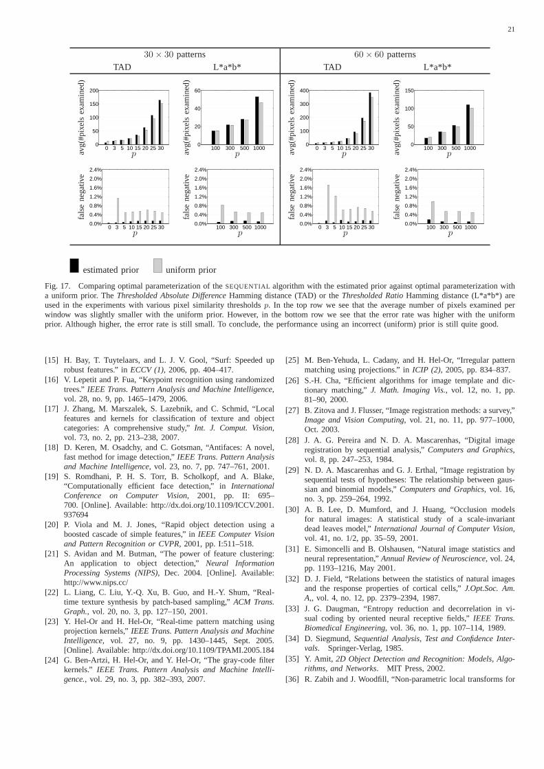
The proposed frameworks are Bayesian,i.e. theyuse a prior on the distribution of the distancesbetween two natural images,P (D = d). The priorcan be estimated, offline, by computing the exactdistance between various patterns and windows.Another option is to use a non-informative prior,i.e. a uniform prior in which the probability for eachpossible distance is equal. Fig. 9 and Fig. 10 showthat the true distribution of distances is not uniform.Nevertheless, Fig. 17 shows that even though weuse an incorrect (uniform) prior to parameterizethe algorithm, we obtain good results. It shouldbe stressed that other fast methods assume certaincharacteristics of images. For example, Hel-Or andHel-Or [23] assume that the first Walsh-Hadamardbasis projections (according to their specific order)contain enough information to discriminate mostimages. Mascarenhas et al. [28], [29] assume thatimages are binary or Gaussian distributed. In ad-dition, they assume that all similar images haveexactly the same pairwise small distance, while alltwo non-similar images have exactly the same largedistance. By explicitly using a prior our method ismore general.

For each distance measure and pattern size, weestimated the prior using a database of 480 naturalimages. First, outlier noise was added to each image.To simulate such noise we chose a different image atrandom from the test database and replaced between0% to 50% (the value was chosen uniformly),with replacement, of the original image pixels withpixels from the different image in the same relativeposition.

For each image we computed the set of distancesbetween two patterns (each a not too smooth ran-domly chosen 2D window from the image before theaddition of the noise) and a sliding window over thenoisy image. The prior that was used is a mixturemodel of this histogram and a uniform prior (witha very small probability for uniformity). We used amixture model as we had almost no observations ofsmall distances.

Fig. 9 shows that priors of the same Hammingdistance for different pattern sizes are similar. Fig.10 shows that as the distance measure becomesmore invariant, the distances are smaller.

0 50 100 150 2000

0.2

0.4

0.6

0.8

1

d=Hamming DistanceP

(D≤

d)

0 200 400 600 8000

0.2

0.4

0.6

0.8

1

d=Hamming Distance

P(D

≤d)

(a) (b)

0 500 1000 1500 20000

0.2

0.4

0.6

0.8

1

d=Hamming Distance

P(D

≤d)

0 1000 2000 30000

0.2

0.4

0.6

0.8

1

d=Hamming Distance

P(D

≤d)

(c) (d)

Fig. 9. Estimated cumulative PDFs of priors ofThresholded AbsoluteDifferenceHamming distance with pixel similarity threshold equal 20(pixels with intensity difference greater than 20 are considered non-similar) for patterns size: (a)15 × 15 (b) 30 × 30 (c) 45 × 45 (d)60 × 60. Note that the shapes of the priors are similar.

VI. EXPERIMENTAL RESULTS

The proposed frameworks were tested on realimages and patterns. The results show that theSEQUENTIAL algorithm is fast and accurate, withor without noise.

Recall that there are two kinds of errors: falsenegative (the event of returningnon-similar on asimilar window), and false positive (the event ofreturningsimilar on a non-similar window). A win-dow is defined as similar to the pattern if and only ifthe Hamming distance between the window and thepattern is smaller or equal to the image similaritythreshold,t. Note that in all the experiments (Figs.1, 3, 4, 5 and 6) the similar windows are alsovisually similar to the pattern.

15

0 1000 2000 30000

0.2

0.4

0.6

0.8

1

d=Hamming Distance

P(D

≤d)

0 1000 2000 30000

0.2

0.4

0.6

0.8

1

d=Hamming Distance

P(D

≤d)

(a) (b)

0 1000 2000 30000

0.2

0.4

0.6

0.8

1

d=Hamming Distance

P(D

≤d)

0 1000 2000 30000

0.2

0.4

0.6

0.8

1

d=Hamming Distance

P(D

≤d)

(c) (d)

Fig. 10. Estimated cumulative PDFs priors ofThresholdedl2 normin L*a*b color spaceHamming distance for60 × 60 patterns, withpixel similarity threshold equal: (a) 100 (b) 300 (c) 500 (d)1000.Note that as the distance measure becomes more invariant (with ahigher pixel similarity threshold), the distances are smaller.

We set the false positive error bound to zero in allexperiments. Setting it to a higher value decreasesthe running time mostly for similar windows. Asit is assumed that similarity between pattern andimage is a rare event, the speedup caused by ahigher bound on the false positive is negligible. Weset the false negative error bound to 0.1%;i.e. outof 1000 similar windows, only one is expected to beclassified as non-similar. Note that this small errorrate enables the large reduction in the running time.

A typical pattern matching task is shown in Fig. 1.A non-rectangular pattern of 2197 pixels was soughtin a sequence of 14, 640x480 pixel frames. Wesearched for windows with aThresholded AbsoluteDifference Hamming distance lower or equal to0.4× 2197, i.e. less than 40% outlier noise such asout of plane rotation, shading, spectral reflectance,occlusion, etc. Two pixels were considered non-similar if their absolute intensity difference wasgreater than 20,i.e. p = 20. The SEQUENTIAL

algorithm was parameterized with P-SPRT (see Sec-tion IV-D), a uniform prior and false negative errorbound of 0.1%. Using the parameterizedSEQUEN-TIAL algorithm, the pattern is found in 9 out of 11frames in which it was present, with an average ofonly 19.70 pixels examined per window instead of2197 needed for the exact distance computation. Ona Pentium 4 3GHz processor, detection of the pat-tern proceeds at 0.022 seconds per frame. The false

positive error rate was 0%. The false negative errorrate was 0.28%. Note that due to image smoothness,there are several similar windows in each framenear the sought object. The errors were mostly dueto missing one of these windows. Although weuse an incorrect (uniform) prior to parameterizethe algorithm, we obtain excellent results. Otherdistances such as cross correlation (CC), normalizedcross correlation (NCC),l1, l2, yielded poor resultseven though they were computed exactly (the com-putation took much longer).

More results are given in Figs. 3, 4, 5 and 6. Allof these results are on 640x480 pixel images and usethe SEQUENTIAL algorithm that was parameterizedwith P-SPRT (see Section IV-D), a uniform priorand false negative error bound of 0.1%. Theseresults are also summarized in Table II. Comparisonof the results using the estimated prior and theuniform prior is given in Fig. 11.

2 3 4 5 60

10

20

30

40

50

Fig.avg(

#fea

ture

ssa

mpl

ed)

2 3 4 5 60.0%

0.4%

0.8%

1.2%

1.6%

Fig.

fals

ene

gativ

e

(a) (b)

estimated prior uniform prior

Fig. 11. Comparing optimal parameterization of theSEQUENTIAL

algorithm with the estimated prior against optimal parameterizationwith a uniform prior in all figure experiments. In (a) the averagenumber of features sampled per window was slightly smaller withthe uniform prior. However, in (b) the error rate was higher with theuniform prior. Although higher, the error rate was still usually small.Thus, the performance using an incorrect (uniform) prior isstill quitegood.

Note that the parameters (pixel similarity thresh-old, p and relative image similarity threshold,t

|A|)

are the same for each kind of distance. These param-eters were chosen as they yield good performancefor images experimentally. They do not necessarilygive the best results. For example, on Fig. 3, usingThresholded Absolute DifferenceHamming distancewith pixel similarity threshold,p equal 100 and theimage similarity threshold,t equal 0, theSEQUEN-TIAL algorithm ran only 0.013 seconds. The averagenumber of pixels examined per window was only2.85 instead of 1089 needed for the exact distancecomputation. The false negative error rate was 0%.

16

Another parameter that can be tuned is which pairsof pixels should setA contain when we use theMonotonic RelationsHamming distance. In all theexperiments that use this distance, the pairs thatwere used are pairs of pixels belonging to edges,i.e.pixels that have a neighbor pixel, where the absoluteintensity value difference is greater than 80. In allthe experiments (except the experiment in Fig. 5)two pixels are considered neighbors if they are inthe same5 × 5 neighborhood. In the experimentin Fig. 5, two pixels are considered neighbors ifthey are in the same11× 11 neighborhood becausepairs in the5 × 5 neighborhood did not describethe pattern well. Thus, all parameters can be tunedfor a specific pattern matching task. However, ourwork shows that for each of the proposed membersof the Image Hamming Distance Family there is astandard set of parameters that usually yield goodperformance.

To illustrate the performance of Bayesian sequen-tial sampling, we also conducted extensive randomtests. The random tests were conducted mainly toillustrate the characteristics of theSEQUENTIAL

algorithm and to compare its parameterization meth-ods.

A test database (different from the trainingdatabase that was used to estimate priors) of 480natural images was used. We consider similar win-dows as windows with a Hamming distance smalleror equal to 50% of their size;e.g.a 60×60 windowis considered similar to a60 × 60 pattern if theHamming distance between them is smaller/equalto 1800.

For comparison we also developed an optimalfixed size sampling algorithm,FIXED SIZE (see Ap-pendix I). Each test of theFIXED SIZE algorithmor the SEQUENTIAL algorithm in Figs. 15, 16 and17 was conducted using a different combination ofmembers of the Image Hamming Distance Fam-ily and different sizes of patterns. For each suchcombination a prior was estimated (see SectionV). In order to parameterize theFIXED SIZE andthe SEQUENTIAL algorithms, we used either theestimated prior or a uniform prior.

Each test of the parameterized algorithms wasconducted by performing 9600 iterations (20 timesfor each image) as follows:

• A random not too smooth 2D window patternwas chosen from one of the images,Im, fromthe test database.

• Outlier noise was added to the image,Im. Tosimulate such noise we chose a different imageat random from the test database and replacedbetween 0% to 50% (the value was chosenuniformly), with replacement, of the originalimage (i.e. Im) pixels with pixels from thedifferent image in the same relative position.

• The pattern was sought for in the noisy image,using the parameterizedSEQUENTIAL algo-rithm or the parameterizedFIXED SIZE algo-rithm.

In each test the false negative error rate and the av-erage number of pixels examined per window werecalculated. Overall, the results can be summarizedas follows:

1) Even with very noisy images theSEQUEN-TIAL algorithm is very fast and accurate.For example, the average number of pixelssampled for pattern matching on60 × 60patterns with additive noise of up to 20 (eachpixel gray value change can range from -20 to+20) and outlier noise of up to 50% was only92.9, instead of 3600. The false negative errorrate was only 0.09% (as mentioned above,the false positive error rate bound was always0%).

2) The SEQUENTIAL algorithm is much fasterthan theFIXED SIZE algorithm, with the sameerror rates. In addition, usually theSEQUEN-TIAL algorithm is less sensitive to incorrectpriors (see Fig. 15).

3) The performance of the near-optimal solution,P-SPRT, is good (see Fig. 16).

4) The average number of features examinedper window is slightly smaller with the uni-form prior. However, the error rate is higher(although still small). Thus, there is not asubstantial difference in performance whenusing an incorrect (uniform) prior (see Figs.11,17).

To further illustrate the robustness of the methodwe conducted another kind of experiment. Five im-age transformations were evaluated: small rotation;small scale change; image blur; JPEG compression;and illumination. The names of the datasets usedarerotation; scale; blur; jpeg; andlight respectively.The blur, jpeg and light datasets were from theMikolajczyk and Schmid paper [14]. Our method isrobust to small but not large geometrical transforms.

17

TABLE II

SUMMARY OF FIGURE RESULTS

Fig. (a) (b) (c) (d) (e) (f) (g)Distance |A| = Max False Average Offline Onlinetype Set Diff Negative Features Time Time

Size (%) (%) Sampled (seconds)(seconds)

1 20TAD(1) 2197 40 0.28 19.70 0.067 0.0223 20TAD(1) 1089 40 1.68 12.07 0.018 0.0194 MR(2) 631 25 0.30 35.28 0.009 0.0215 MR(2) 9409 25 0.45 39.98 1.219 0.0376 LD-20TAD(3) 714 5 0.20 16.98 0.007 0.064

(a) Distance types:1) 20TAD - Thresholded Absolute Difference, with threshold(p) of 20.2) MR - Monotonic Relations.3) LD-20TAD - Local Deformationsvariant ofThresholded Absolute Difference, with threshold(p) of 20.

(b) Size of the set of spatial coordinates of features,i.e. number of pixels inThresholded Absolute Differencedistances, or number of pairs

of pixels in Monotonic RelationsHamming distance.

(c) Maximum percentage of pixels, or pairs of pixels, that can be different in similar windows. For example, in Fig. 1, similar windows

Hamming distance is less than( 40100

)2197 = 878.

(d) The false negative error rate (percentage of similar windows that the algorithm returned as non-similar). For example, in Fig. 1, on

average out of 10000 similar windows, 28 were missed. Note that due to image smoothness, there were several similar windows in each

image near each sought object. The errors were mostly due to missing one of these windows.

(e) Average number of pixels sampled inThresholded Absolute Differencedistances, or average number of pairs of pixels sampled in

Monotonic RelationsHamming distances.

(f) Running time of the parameterization of theSEQUENTIAL algorithm. In addition, inMonotonic Relationsdistances it also includes the

running time of finding the pairs of pixels that belong to edges.

(g) Running time of pattern detection using theSEQUENTIAL algorithm, where each image is 640x480 pixels in size.

Thus, it did not perform well on the geometricalchanges datasets from the Mikolajczyk and Schmidpaper [14]. We created two datasets with smallgeometrical transforms: ascaledataset that contains22 images with an artificial scale change from 0.9to 1.1 in jumps of 0.01; and arotation datasetthat contains 22 images with an artificial in-planerotation from -10 to 10 in jumps of 1 (see forexample Fig. 14).

For each collection, ten rectangular patterns werechosen from the image with no transformation. Thepairs that were used in the set of each pattern werepairs of pixels belonging to edges,i.e. pixels thathad a neighbor pixel, where the absolute intensityvalue difference was greater than 80. Two pixels,(x2, y2), (x1, y1) are considered neighbors if theirl∞ distance:max(|x1 − x2|, |y1 − y2|) is smalleror equal to 2. We searched for windows with aMonotonic RelationsHamming distance lower orequal to0.25 × |A|. In each image we considered

only the window with the minimum distance assimilar, because we knew that the pattern occurredonly once in the image. TheSEQUENTIAL algorithmwas parameterized using P-SPRT (see Section IV-D) with input of a uniform prior and a false negativeerror bound of 0.1%. We repeated each search of apattern in an image 1000 times.

We defined two new notions of performance: missdetection error rate and false detection error rate.As we know the true homographies between theimages, we know where the pattern pixels are inthe transformed image. We denote a correct matchas one that covers at least 80% of the transformedpattern pixels. A false match is one that coversless than 80% of the transformed pattern pixels.Note that there is also an event of no detectionat all if the SEQUENTIAL algorithm does not findany window with aMonotonic RelationsHammingdistance lower or equal to0.25 × |A|. The missdetection error rate is the percentage of searches

18

of a pattern in an image that does not yield acorrect match. The false detection error rate is thepercentage of searches of a pattern in an imagethat yields a false match. Note that in the randomtests that illustrated the performance of the Bayesiansequential sampling, it was not possible to use theseerror notions. In these tests we used a large numberof patterns that were chosen randomly, thus wecould not guarantee that the patterns did not occurmore than once in these test images.

In the light and jpeg tests, the performance wasperfect; i.e. 0% miss detection rate and 0% falsedetection rate. In theblur test, only one patternwas not found correctly in the most blurred image(see Fig. 14). The miss detection rate and falsedetection rate for this specific case was 99.6%. In allother patterns and images in theblur test, the missdetection rate and false detection rate was 0%. Inthe scaletest, there was only one pattern with falsedetection in two images with scale 0.9 and 0.91. Inthe rotation test, there was only one pattern withfalse detection in images with rotation smaller than-2 or larger than +2. Miss detection rates in thescaleandrotation tests (see Fig. 12) were dependenton the pattern. If the scale change or rotation wasnot too big, the pattern was found correctly.

The average number of pair of pixels that theSEQUENTIAL algorithm sampled per window wasnot larger than 45 in all of the above tests. Theaverage was 29.38 and the standard deviation was4.22. In general, the number of samples decreasedwith image smoothness;e.g.it decreased with imageblur, lack of light and JPEG compression (seefor example Fig. 13). Note that theSEQUENTIAL

algorithm using theMonotonic RelationsHammingdistance stops as soon as there are not enough edgepairs of pixels in the same spatial position as inthe pattern. Smoothness decreases the number ofedge pairs of pixels; thus it decreases the averagenumber of samples that theSEQUENTIAL algorithmsamples.

Finally, Table III compares the running time ofthe two kinds of offline phases.i.e. it compares therunning time of finding the optimal decision matrix(see Section IV-C) with the running time of find-ing the P-SPRT (near-optimal) decision matrix (seeSection IV-D). Thus finding the P-SPRT decisionmatrix is an order of magnitude faster. All runs wereconducted on a Pentium 4 3GHz processor.

Miss Detection Rate 100% <1% 0%

scale

pat

tern

nu

mb

er

0.9 0.92 0.94 0.96 0.98 1 1.02 1.04 1.06 1.08 1.1

123456789

10

0.4

0.2

(a)

rotation

pat

tern

nu

mb

er

-10 -8 -6 -4 -2 0 2 4 6 8 10

123456789

10

0.50.3

(b)

Fig. 12. (a) Miss detection error rates on thescale test. (b) Missdetection error rates on therotation test.

12345678910

JPEG compression level

#av

gsa

mp

les

0 1 2 3 4 55

10

15

20

25

30

35

Fig. 13. Average number of pairs of pixels that theSEQUENTIAL

algorithm sampled per window in thejpeg test.

VII. CONCLUSIONS

This paper introduced the “Image HammingDistance Family”. We also presented a Bayesianframework for sequential hypothesis testing on fi-nite populations that designs optimal sampling al-gorithms. Finally, we detailed a framework thatquickly designs a near-optimal sampling algorithm.We showed that the combination of an optimal ora near-optimal sampling algorithm and members ofthe Image Hamming Distance Family gives a robust,real time, pattern matching method.

Extensive random tests show that theSEQUEN-TIAL algorithm performance is excellent. TheSE-QUENTIAL algorithm is much faster than theFIXED SIZE algorithm with the same error rates. Inaddition, theSEQUENTIAL algorithm is less sensi-

19

TABLE III

OFFLINE RUNNING TIME COMPARISON

|A| - features’ coordinates set size 500 1000 1500 2000 2500 3000

Offline P-SPRT (seconds) 0.005 0.018 0.042 0.075 0.14 0.17Offline optimal (seconds) 7.510 49.220 154.520 653.890 2012.40 3504.97

(a)

(b)

Fig. 14. (a) The single false detection event on theblur test. (b) Anexample of detection on therotation test. The image is 5 artificiallyin-plane rotated.

tive to incorrect priors. The performance of the near-optimal solution, P-SPRT, is good. It is noteworthythat performance using an incorrect (uniform) priorto parameterize theSEQUENTIAL algorithm is stillquite good.

The technique explained in this paper was de-scribed in an image pattern matching context. How-ever we emphasize that this is an example appli-cation. Sequential hypothesis tests on finite popula-tions are used in quality control (e.g.[53]) , sequen-tial mastery testing (e.g. [54], [55]) and possiblymore fields. Thus the method can be used as is toproduce optimal sampling schemes in these fields.

The project homepage is at:http://www.cs.huji.ac.il/∼ofirpele/hs

ACKNOWLEDGMENT

We thank Professor Ester Samuel-Cahn for an en-lightening discussion, Refael Vivanti for optimiza-tion and coding assistance and to Liat Pele, AmichaiZisken, Ori Maoz, Amit Gruber, Amnon Aaronsohn,Aviv Hurvitz, Eran Maryuma and Refael Vivanti forproofreading.

REFERENCES

[1] A. Wald, Sequential Analysis. Wiley, New York, 1947.[2] D. I. Barnea and H. F. Silverman, “A class of algorithms for

fast digital image registration,”IEEE Trans. Computer, vol. 21,no. 2, pp. 179–186, Feb. 1972.

[3] J. Matas and O. Chum, “Randomized ransac with sequentialprobability ratio test,” inProc. IEEE International Conferenceon Computer Vision (ICCV), vol. 2, October 2005, pp. 1727–1732.

[4] J. Sochman and J. Matas, “Waldboost - learning for timeconstrained sequential detection,” inProc. of Conference onComputer Vision and Pattern Recognition (CVPR), vol. 2, June2005, pp. 150–157.

[5] P. E. Anuta, “Spatial registration of multispectral andmultitem-poral digital imagery using fast fourier transform,”IEEE Trans.Geoscience Electronics, vol. 8, pp. 353–368, 1970.

[6] J. P. Lewis, “Fast normalized cross-correlation,” Sept. 021995. [Online]. Available: http://www.idiom.com/∼zilla/Work/nvisionInterface/nip.pdf

[7] A. J. Ahumada, “Computational image quality metrics: Areview.” Society for Information Display International Sympo-sium, vol. 24, pp. 305–308, 1998.

[8] B. Girod, Digital Images and Human Vision, ”Whats wrongwith the mean-squared error?”. MIT press, 1993, ch. 15.

[9] A. M. Eskicioglu and P. S. Fisher, “Image quality measuresand their performance,”IEEE Trans. Communications, vol. 43,no. 12, pp. 2959–2965, 1995.

[10] S. Santini and R. C. Jain, “Similarity measures,”IEEE Trans.Pattern Analysis and Machine Intelligence, vol. 21, no. 9, pp.871–883, Sept. 1999.

[11] B. D. Lucas and T. Kanade, “An iterative image registrationtechnique with an application to stereo vision,” inImageUnderstanding Workshop, 1981, pp. 121–130.

[12] J. Matas, O. Chum, M. Urban, and T. Pajdla, “Robust widebaseline stereo from maximally stable extremal regions,” inProceedings of the British Machine Vision Conference, vol. 1,London, UK, September 2002, pp. 384–393.

[13] D. G. Lowe, “Distinctive image features from scale-invariantkeypoints,” Int. J. Comput. Vision, vol. 60, no. 2, pp. 91–110,2004.

[14] K. Mikolajczyk and C. Schmid, “A performance evaluation oflocal descriptors,”IEEE Trans. Pattern Analysis and MachineIntelligence, vol. 27, no. 10, pp. 1615–1630, 2005.

20

30 × 30 patterns 60 × 60 patterns

estimated prior uniform prior estimated prior uniform prior

0 3 5 10 15 20 25 300

100

200

300

pavg(

#pix

els

exam

ined

)

0 3 5 10 15 20 25 300

100

200

300

pavg(

#pix

els

exam

ined

)

0 3 5 10 15 20 25 300

200

400

600

800

pavg(

#pix

els

exam

ined

)

0 3 5 10 15 20 25 300

200

400

600

800

pavg(

#pix

els

exam

ined

)

0 3 5 10 15 20 25 300.0%

0.1%

0.2%

p

fals

ene

gativ

e

0 3 5 10 15 20 25 300.0%

0.4%

0.8%

1.2%

1.6%

2.0%

p

fals

ene

gativ

e

0 3 5 10 15 20 25 300.0%

0.1%

0.2%

p

fals

ene

gativ

e

0 3 5 10 15 20 25 300.0%

0.4%

0.8%

1.2%

1.6%

2.0%

p

fals

ene

gativ

e

FIXED SIZE algorithm SEQUENTIAL algorithm

Fig. 15. Comparing theFIXED SIZE algorithm with theSEQUENTIAL algorithm. Both algorithms were parametrized using the estimatedor the uniform prior. TheSEQUENTIAL algorithm is much faster than theFIXED SIZE algorithm, with the same error rates. In addition, theSEQUENTIAL algorithm is less sensitive to incorrect (uniform) priors.In the top row we see that the average number of pixels examined perwindow was smaller using theSEQUENTIAL algorithm. In the bottom row we see that the error rate was thesame in both algorithms. Wecan also see that theSEQUENTIAL algorithm is less sensitive to incorrect (uniform) priors (note that when the pixel similarity threshold isequal to 0, 3 and 5 the number of samples using theFIXED SIZE algorithm increases when using the uniform prior). All tests were conductedusing theThresholded Absolute DifferenceHamming distance with various pixel similarity thresholdsp.

30 × 30 patterns 60 × 60 patternsTAD L*a*b* TAD L*a*b*

0 3 5 10 15 20 25 300

50

100

150

pavg(

#pix

els

exam

ined

)

100 300 500 10000

20

40

60

pavg(

#pix

els

exam

ined

)

0 3 5 10 15 20 25 300

100

200

300

400

pavg(

#pix

els

exam

ined

)

100 300 500 10000

50

100

pavg(

#pix

els

exam

ined

)

0 3 5 10 15 20 25 300.0%

0.1%

0.2%

0.3%

p

fals

ene

gativ

e

100 300 500 10000.0%

0.1%

0.2%

0.3%

p

fals

ene

gativ

e

0 3 5 10 15 20 25 300.0%

0.1%

0.2%

0.3%

p

fals

ene

gativ

e

100 300 500 10000.0%

0.1%

0.2%

0.3%

p

fals

ene

gativ

e

P-SPRT OPT

Fig. 16. Comparing the two parameterizations of theSEQUENTIAL algorithm: optimal and P-SPRT. TheThresholded Absolute DifferenceHamming distance (TAD) or theThresholded RatioHamming distance (L*a*b*) are used in the experiments with various pixel similaritythresholdsp. All parameterizations were done with the estimated prior.P-SPRT samples a little more, with slightly smaller error rates.

21

30 × 30 patterns 60 × 60 patterns

TAD L*a*b* TAD L*a*b*

0 3 5 10 15 20 25 300

50

100

150

200

pavg(

#pix

els

exam

ined

)

100 300 500 10000

20

40

60

pavg(

#pix

els

exam

ined

)

0 3 5 10 15 20 25 300

100

200

300

400

pavg(

#pix

els

exam

ined

)

100 300 500 10000

50

100

150

pavg(

#pix

els

exam

ined

)

0 3 5 10 15 20 25 300.0%

0.4%

0.8%

1.2%

1.6%

2.0%

2.4%

p

fals

ene

gativ

e

100 300 500 10000.0%

0.4%

0.8%

1.2%

1.6%

2.0%

2.4%

p

fals

ene

gativ

e

0 3 5 10 15 20 25 300.0%

0.4%

0.8%

1.2%

1.6%

2.0%

2.4%

p

fals

ene

gativ

e

100 300 500 10000.0%

0.4%

0.8%

1.2%

1.6%

2.0%

2.4%

p

fals

ene

gativ

e

estimated prior uniform prior

Fig. 17. Comparing optimal parameterization of theSEQUENTIAL algorithm with the estimated prior against optimal parameterization witha uniform prior. TheThresholded Absolute DifferenceHamming distance (TAD) or theThresholded RatioHamming distance (L*a*b*) areused in the experiments with various pixel similarity thresholds p. In the top row we see that the average number of pixels examined perwindow was slightly smaller with the uniform prior. However, in the bottom row we see that the error rate was higher with the uniformprior. Although higher, the error rate is still small. To conclude, the performance using an incorrect (uniform) prior is still quite good.

[15] H. Bay, T. Tuytelaars, and L. J. V. Gool, “Surf: Speeded uprobust features.” inECCV (1), 2006, pp. 404–417.

[16] V. Lepetit and P. Fua, “Keypoint recognition using randomizedtrees.”IEEE Trans. Pattern Analysis and Machine Intelligence,vol. 28, no. 9, pp. 1465–1479, 2006.

[17] J. Zhang, M. Marszalek, S. Lazebnik, and C. Schmid, “Localfeatures and kernels for classification of texture and objectcategories: A comprehensive study,”Int. J. Comput. Vision,vol. 73, no. 2, pp. 213–238, 2007.

[18] D. Keren, M. Osadchy, and C. Gotsman, “Antifaces: A novel,fast method for image detection,”IEEE Trans. Pattern Analysisand Machine Intelligence, vol. 23, no. 7, pp. 747–761, 2001.

[19] S. Romdhani, P. H. S. Torr, B. Scholkopf, and A. Blake,“Computationally efficient face detection,” inInternationalConference on Computer Vision, 2001, pp. II: 695–700. [Online]. Available: http://dx.doi.org/10.1109/ICCV.2001.937694

[20] P. Viola and M. J. Jones, “Rapid object detection using aboosted cascade of simple features,” inIEEE Computer Visionand Pattern Recognition or CVPR, 2001, pp. I:511–518.

[21] S. Avidan and M. Butman, “The power of feature clustering:An application to object detection,”Neural InformationProcessing Systems (NIPS), Dec. 2004. [Online]. Available:http://www.nips.cc/

[22] L. Liang, C. Liu, Y.-Q. Xu, B. Guo, and H.-Y. Shum, “Real-time texture synthesis by patch-based sampling,”ACM Trans.Graph., vol. 20, no. 3, pp. 127–150, 2001.

[23] Y. Hel-Or and H. Hel-Or, “Real-time pattern matching usingprojection kernels,”IEEE Trans. Pattern Analysis and MachineIntelligence, vol. 27, no. 9, pp. 1430–1445, Sept. 2005.[Online]. Available: http://dx.doi.org/10.1109/TPAMI.2005.184

[24] G. Ben-Artzi, H. Hel-Or, and Y. Hel-Or, “The gray-code filterkernels.” IEEE Trans. Pattern Analysis and Machine Intelli-gence., vol. 29, no. 3, pp. 382–393, 2007.

[25] M. Ben-Yehuda, L. Cadany, and H. Hel-Or, “Irregular patternmatching using projections.” inICIP (2), 2005, pp. 834–837.

[26] S.-H. Cha, “Efficient algorithms for image template anddic-tionary matching,”J. Math. Imaging Vis., vol. 12, no. 1, pp.81–90, 2000.

[27] B. Zitova and J. Flusser, “Image registration methods:a survey,”Image and Vision Computing, vol. 21, no. 11, pp. 977–1000,Oct. 2003.

[28] J. A. G. Pereira and N. D. A. Mascarenhas, “Digital imageregistration by sequential analysis,”Computers and Graphics,vol. 8, pp. 247–253, 1984.

[29] N. D. A. Mascarenhas and G. J. Erthal, “Image registration bysequential tests of hypotheses: The relationship between gaus-sian and binomial models,”Computers and Graphics, vol. 16,no. 3, pp. 259–264, 1992.

[30] A. B. Lee, D. Mumford, and J. Huang, “Occlusion modelsfor natural images: A statistical study of a scale-invariantdead leaves model,”International Journal of Computer Vision,vol. 41, no. 1/2, pp. 35–59, 2001.

[31] E. Simoncelli and B. Olshausen, “Natural image statistics andneural representation,”Annual Review of Neuroscience, vol. 24,pp. 1193–1216, May 2001.

[32] D. J. Field, “Relations between the statistics of natural imagesand the response properties of cortical cells,”J.Opt.Soc. Am.A,, vol. 4, no. 12, pp. 2379–2394, 1987.

[33] J. G. Daugman, “Entropy reduction and decorrelation invi-sual coding by oriented neural receptive fields,”IEEE Trans.Biomedical Engineering, vol. 36, no. 1, pp. 107–114, 1989.

[34] D. Siegmund,Sequential Analysis, Test and Confidence Inter-vals. Springer-Verlag, 1985.

[35] Y. Amit, 2D Object Detection and Recognition: Models, Algo-rithms, and Networks. MIT Press, 2002.

[36] R. Zabih and J. Woodfill, “Non-parametric local transforms for

22

computing visual correspondence,” inECCV, 1994, pp. 151–158.

[37] B. Cyganek, “Comparison of nonparametric transformationsand bit vector matching for stereo correlation.” inIWCIA, 2004,pp. 534–547.

[38] Q. Lv, M. Charikar, and K. Li, “Image similarity search withcompact data structures,” inCIKM. New York, NY, USA:ACM Press, 2004, pp. 208–217.

[39] M. Ionescu and A. Ralescu, “Fuzzy hamming distance in acontent-based image retrieval system,” inFUZZ-IEEE, 2004.

[40] A. Bookstein, V. A. Kulyukin, and T. Raita, “Generalizedhamming distance,”Inf. Retr., vol. 5, no. 4, pp. 353–375, 2002.

[41] A. Abhyankar, L. A. Hornak, and S. Schuckers, “Biorthogonal-wavelets-based iris recognition,” A. K. Jain and N. K. Ratha,Eds., vol. 5779, no. 1. SPIE, 2005, pp. 59–67. [Online].Available: http://link.aip.org/link/?PSI/5779/59/1

[42] P. Hough, “A method and means for recognizing complexpatterens,”U.S. Patent 3,069,654, 1962.

[43] S. D. Blostein and T. S. Huang, “Detecting small, movingobjects in image sequences using sequential hypothesis testing,”IEEE Trans. Signal Processing, vol. 39, no. 7, pp. 1611–1629,1991.

[44] D. Shaked, O. Yaron, and N. Kiryati, “Deriving stoppingrulesfor the probabilistic hough transform by sequential analysis,”Comput. Vis. Image Underst., vol. 63, no. 3, pp. 512–526, 1996.

[45] A. Amir and M. Lindenbaum, “A generic grouping algorithmand its quantitative analysis.”IEEE Trans. Pattern Analysis andMachine Intelligence., vol. 20, no. 2, pp. 168–185, 1998.

[46] M. A. Fischler and R. C. Bolles, “Random sample consensus: aparadigm for model fitting with applications to image analysisand automated cartography,”Commun. ACM, vol. 24, no. 6, pp.381–395, 1981.

[47] H. Gharavi and M. Mills, “Blockmatching motion estima-tion algorithms-new results,”IEEE Trans. Circuits Syst. VideoTechn., vol. 37, no. 5, pp. 649–651, 1990.

[48] G. Wyszecki and W. S. Stiles,Color Science: Concepts andMethods, Quantitative Data and Formulae. Wiley, 1982.

[49] R. Brunelli and T. Poggio, “Face recognition: Featuresversustemplates,”IEEE Trans. Pattern Analysis and Machine Intelli-gence., vol. 15, no. 10, pp. 1042–1052, 1993.

[50] Z. Govindarajulu,Sequential Statistical Procedures. AcademicPress, 1975, pp. 534–536.

[51] A. Wald and J. Wolfowitz, “Optimum character of the sequen-tial probability ratio test,”Ann. Math. Stat., vol. 19, pp. 326–339, 1948.

[52] E. L. Lehmann,Testing Statistical Hypotheses. John Wiley &Sons, 1959, pp. 104–110.

[53] H.-J. Mittag and H. Rinne,Statistical Methods of QualityAssurance. Chapman and Hall, 1993.

[54] H. J. Vos, “A bayesian sequential procedure for determiningthe optimal number of interrogatory examples for concept-learning,” Computers in Human Behavior, vol. 23, no. 1, pp.609–627, January 2007.

[55] C. Lewis and K. Sheehan, “Using bayesian decision theoryto design a computerized mastery test,”Applied PsychologicalMeasurement, vol. 14, no. 4, pp. 367–386, 1990.

Ofir Pele received the BSc degree in computerscience and life science and the MSc degreein computer science from the Hebrew Univer-sity of Jerusalem, Israel, in 2003 and 2005,respectively. He is currently a PhD student incomputer science at the Hebrew University ofJerusalem. His research interests include com-puter vision, sequential analysis and Bayesianstatistics.

Michael Werman Ph.D. 1986, The HebrewUniversity, currently professor of computerscience at The Hebrew University. His researchhas is mainly in designing computer algo-rithms and mathematical tools for analyzing,understanding and synthesizing pictures.

23

APPENDIX IFIXED SIZE FRAMEWORK

We first present theFIXED SIZE algorithm thattests for similarity using a fixed size sample. Thenwe evaluate its performance. Finally we show howto find the optimal parameters for theFIXED SIZE

algorithm.

A. TheFIXED SIZE algorithm

The FIXED SIZE algorithm has threshold param-etersl, u and a fixed sample sizen. The frameworkcomputes optimall, u and n offline. Then, thealgorithm can quickly decide whether a pattern anda window are similar;i.e. if their Hamming distanceis smaller or equal to the image similarity threshold,t.

The algorithm samplesn corresponding featuresfrom the pattern and the window, computes theirHamming distance and decides according to theresult whether to returnsimilar, non-similar or tocompute the exact distance.

Algorithm 6 FIXED SIZEl,u,n,t(pattern,window, A)k ⇐ 0for i = 1 to n do

random sample uniformly and without replace-ment (x, y)m from A

k ⇐ k + sim(pattern, window, (x, y)m)if k ≤ l then

return similarif k ≥ u then

return non-similarreturn (HammingDistanceA(pattern, window)) ≤ t

B. Evaluating performance for fixed parametersl, u, n

The performance of the algorithm is defined by itsexpected number of examined features and its errorprobabilities. The computation is similar to the onein the SEQUENTIAL algorithm (see Section IV):

Pl,u,n(false negative) =

∑nk=u

(n

k

)ΩS[k, n]

P (D ≤ t)(10)

Pl,u,n(false positive) =

∑lk=0

(n

k

)ΩNS[k, n]

P (D > t)(11)

El,u,n(#examined features) =

n + P (compute exact)(|A| − n) =

n +u−1∑

k=l+1

(n

k

)(ΩS[k, n] + ΩNS [k, n])(|A| − n)

(12)

C. Finding optimal parametersl, u, n for the algo-rithm

We first find optimal thresholdsl, u for a givensample size,n. Our goal is to minimize the expectednumber of examined features given bounds on theerror probabilities,α, β:

arg minl,u

El,u(#examined features)

s.t :

Pl,u(false negative) ≤ α

Pl,u(false positive) ≤ β

Fixed number of samplesn

(13)

Pl,u(false negative) (Eq. 10) monotonically de-creases with the thresholdu (the number of non-negative summands decreases).Pl,u(false positive)(Eq. 11) monotonically increases with the thresholdl (the number of non-negative summands increases).El,u(#examined features) (Eq. 12) monotonicallydecreases with the thresholdu and monotonicallyincreases with the thresholdl. Thus, we wantl tobe as large as possible, andu to be as small aspossible.

The algorithm that chooses the optimalu, Alg.7, starts by takingu = n + 1 and decreases it untilPl,u(false negative) is too high. The algorithm thatchooses optimall, Alg. 8 starts by takingl = −1and increases it untilPl,u(false positive) is too high.

Algorithm 7 opt u(n, t, α, P )err ⇐ 0nCk ⇐ 1 The current n choose kfor k = n to 0 do

err ⇐ err + nCk × ΩS [k,n]P (D≤t)

if err > α thenreturn k + 1

nCk ⇐ nCk ×(

kn−k+1

)

return k

24

Algorithm 8 otp l(n, t, β, P )err ⇐ 0nCk ⇐ 1 The current n choose kfor k = 0 to n do

err ⇐ err + nCk × ΩNS [k,n]P (D>t)

if err > β thenreturn k − 1

nCk ⇐ nCk ×(

n−kk+1

)

return k

In order to find the optimaln we compute optimall, u and the expected number of examined featuresfor eachn = 1 . . . |A|. Finally, we choose thenthat minimizes the expected number of examinedfeatures. Note that the search can be terminatedas soon as the current minimum of the expectednumber of examined features is smaller thann.

The intermediate sumsΩS [k, n] and ΩNS[k, n](see Eq. 2) are computed for all possiblek andn with a dynamic programming algorithm with atime complexity of O(|A|3). The algorithms thatcompute optimall, u for eachn (Algs. 8, 7) havea time complexity of O(|A|). These algorithms runa maximum of |A| times. Thus, finding optimaln, l, u has a time complexity of O(|A|3). It should benoted that the search for the optimal parameters isdone offline. The user can employ theFIXED SIZE

algorithm parameterized with the optimall, u, n, toquickly detect patterns in images.

APPENDIX IIHOUGH TRANSFORM COMPUTATION OF

HAMMING DISTANCE

For simplicity we show how to use the Houghtransform [42] to compute theThresholded AbsoluteDifference Hamming Distance (see Section III-B)between a pattern and all windows in a 256 graylevel image. The generalization to other membersof the Image Hamming Distance Family is easy. Wealso analyze its time complexity.

List of symbols:A = Set that contains spatial coordinatesof pixels. |A| is the size of this set.RIm = Number of rows in large image.CIm = Number of columns in large image.L = A 256 array that contains lists of allpixel coordinates in the pattern that aresimilar to a specific gray value.

p = Pixel similarity threshold of theThresholded Absolute DifferenceHam-ming Distance.H = The Thresholded Absolute DifferenceHamming Distance Map,i.e. H[r, c] istheThresholded Absolute DifferenceHam-ming Distance between the pattern and thewindow of the imageIm whose top leftpixel is [r, c].

Algorithm 9 HoughTAD(pattern,image,p)L[0 . . . 255] ⇐ empty list of indices.for (x, y) ∈ A do

for g = (pattern[x, y]−p) to (pattern[x, y]+p)do

L[g].insert([x, y])H[0 . . . RIm, 0 . . . CIm] ⇐ |A|for r = 1 to RIm do

for c = 1 to CIm dofor it = (L[image[r, c]].begin) to(L[image[r, c]].end) do

H[r−it.r, c−it.c] ⇐ H[r−it.r, c−it.c]−1

The first stage of Algorithm 9 which computesthe array of lists, L has a time complexity ofO(|A|p). The second stage which computes theHamming distance map, H has an expected timecomplexity of O(RImCIm(|A| − E[D])), whereD is the random variable of the Hamming dis-tance. Total expected time complexity isO(|A|p +RImCIm(|A|−E[D])). Average expected time com-plexity per window isO( |A|p

CImRIm+ |A| − E[D]).

Since usually |A|pCImRIm

is negligible the averageexpected time complexity per window isO(|A| −E[D])

APPENDIX IIICOMPUTATION OF PROBABILITIES OF THE

SEQUENTIAL ALGORITHM

List of symbols:• M = SEQUENTIAL algorithm decision matrix.

M [k, n] is the algorithm decision after sam-pling k non-similar corresponding features outof a total ofn sampled corresponding features.The decision can beNS=return non-similar,S=returnsimilar or C=continue sampling. Seethe graphical representation in Fig. 8.

• D = Random variable of the Hamming dis-tance.

25

• t = Image similarity threshold,i.e. if the Ham-ming distance of two images is smaller orequal to t, then the images are consideredsimilar. Otherwise, the images are considerednon-similar.

• ΨM [k, n] = Number of paths from the point(0, 0) to the point(k, n) that do not touch astopping point (S, NS) in Fig. 8 on page 10.

• ek,n= The event of samplingk non-similarcorresponding features out of a total ofn

sampled corresponding features, in any spe-cific order (for example, where the non-similarcorresponding features are sampled first). Notethat all orders of sampling have the sameprobability. See Eq. 1 on page 10.

• ΩS[k, n], ΩNS[k, n] = Intermediate sums de-fined in Eq. 2 on page 11.

PM (false negative) (14)

= PM (returnnon-similar|images are similar) (15)

= PM (returnnon-similar|D ≤ t) (16)

=

|A|∑

d=0

PM (returnnon-similar, D = d|D ≤ t) (17)

=1

P (D ≤ t)

t∑

d=0

PM (returnnon-similar, D = d) (18)

=1

P (D ≤ t)

t∑

d=0

∑

(k,n):M(k,n)=NS

Ψ[k, n]P (ek,n, D = d)

(19)

=1

P (D ≤ t)

∑

(k,n):M(k,n)=NS

Ψ[k, n]

t∑

d=0

P (ek,n, D = d)

(20)

=1

P (D ≤ t)

∑

(k,n):M(k,n)=NS

Ψ[k, n]ΩS[k, n] (21)

PM (false positive) (22)

= PM (returnsimilar|images are non-similar) (23)

= PM (returnsimilar|D > t) (24)

=

|A|∑

d=0

PM (returnsimilar, D = d|D > t) (25)

=1

P (D > t)

|A|∑

d=t+1

PM (returnsimilar, D = d) (26)

=1

P (D > t)

|A|∑

d=t+1

∑

(k,n):M(k,n)=S

Ψ[k, n]P (ek,n, D = d)

(27)

=1

P (D > t)

∑

(k,n):M(k,n)=S

Ψ[k, n]

|A|∑

d=t+1

P (ek,n, D = d)

(28)

=1

P (D > t)

∑

(k,n):M(k,n)=S

Ψ[k, n]ΩNS [k, n] (29)

EM [#samples] (30)

=

|A|∑

d=0

EM [#samples, D = d] (31)

=

|A|∑

d=0

∑

(k,n):M(k,n)∈S,NS

Ψ[k, n]P (ek,n, D = d)n (32)

=∑

(k,n):M(k,n)∈S,NS

Ψ[k, n](ΩS [k, n] + ΩNS [k, n])n (33)

APPENDIX IVCOMPUTATION OF EXPECTED ADDITIVE LOSS IN

THE BACKWARD INDUCTION ALGORITHM

Let w1 and w0 be the loss weights for falsepositive error and false negative error respectively.The expected additive loss for each decision giventhat we sampledn samples, out of whichk werenon-similar is:

E[addLoss(S)|k, n] = P (D > t|ek,n)w1 (34)

=P (D > t, ek,n)

P (ek,n)w1 (35)

=

∑|A|d=t+1 P (D = d, ek,n)∑|A|

d=0 P (D = d, ek,n)w1 (36)

=ΩNS [k, n]

ΩS [k, n] + ΩNS [k, n]w1 (37)

E[addLoss(NS)|k, n] = P (D ≤ t|ek,n)w0 (38)

=P (D ≤ t, ek,n)

P (ek,n)w0 (39)

=

∑t

d=0 P (D = d, ek,n)∑|A|

d=0 P (D = d, ek,n)w0 (40)

=ΩS [k, n]

ΩS [k, n] + ΩNS [k, n]w0 (41)

26

E[addLoss(C)|k, n] = (42)

=1 + P (next feature similar|ek,n)addLossOpt(k, n + 1)+(43)

P (next feature non-similar|ek,n)addLossOpt(k + 1, n + 1)(44)

=1 +P (next feature similar, ek,n)

P (ek,n)addLossOpt(k, n + 1)+

(45)

P (next feature non-similar, ek,n)

P (ek,n)addLossOpt(k + 1, n + 1)

(46)

=1 +P (ek,n+1)

P (ek,n)addLossOpt(k, n + 1)+ (47)

P (ek+1,n+1)

P (ek,n)addLossOpt(k + 1, n + 1) (48)

=1 +ΩS [k, n + 1] + ΩNS[k, n + 1]

ΩS [k, n] + ΩNS[k, n]addLossOpt(k, n + 1)+

(49)

ΩS [k + 1, n + 1] + ΩNS[k + 1, n + 1]

ΩS [k, n] + ΩNS[k, n]× (50)

addLossOpt(k + 1, n + 1) (51)

APPENDIX VBACKWARD INDUCTION SOLUTION THEOREMS

Theorem 1:Let M∗ be a decision matrix whichis the solution to Eq. 8. Then it is the solution tothe original minimization problem Eq. 7 withα =PM∗(false negative) andβ = PM∗(false positive).

Proof: Let M ′ be another decision matrix ofthe same size and smaller/equal error probabilities.Then:

loss(M∗, w0, w1)

= PM∗(false negative)P (D ≤ t)w0+ (52)

PM∗(false positive)P (D > t)w1+

EM∗ [#samples]

≤ PM ′ (false negative)P (D ≤ t)w0+ (53)

PM ′ (false positive)P (D > t)w1+

EM ′ [#samples]

≤ PM∗(false negative)P (D ≤ t)w0+ (54)

PM∗(false positive)P (D > t)w1+ (55)

EM ′ [#samples]

m

EM∗ [#samples] ≤ EM ′ [#samples]

Explanations:(52) Definition of theloss function (Eq. 8)(53) M∗ is optimal (Eq. 8)(54) PM ′(false negative) ≤ PM∗(false negative)

(55) PM ′(false positive) ≤ PM∗(false positive)

Theorem 2:Let M∗ be the optimal decision ma-trix returned by Alg. 3 for somew0, w1. If w0 =

|A|αP (D≤t)

then PM∗(false negative) ≤ α. If w1 =|A|

βP (D>t)thenPM∗(false positive) ≤ β

Proof: Let M ′ be a decision matrix such thatthe SEQUENTIAL algorithm parametrized with italways returns the true answer by sampling all thecorresponding features. Then:

|A| = Loss(M ′, w0, w1) (56)

≥ Loss(M∗, w0, w1) (57)

≥ PM∗(false negative)P (D ≤ t)w0 (58)

= PM∗(false negative)P (D ≤ t)|A|

αP (D ≤ t)(59)

m

PM∗(false negative) ≤ α

Explanations:(56) loss for taking all samples(57) M∗ is optimal(58) part of sum of non-negatives

(59) w0 = |A|αP (D≤t)

The proof of if w1 = |A|βP (D>t)

thenPM∗(false positive) ≤ β is similar.

APPENDIX VICOMPUTATION OF PROBABILITIES FOR THE

P-SPRTFRAMEWORK

The likelihood ratio derivation:

λ(ek,n) =P (ek,n|D > t)

P (ek,n|D ≤ t)(60)

=

∑|A|d=t+1 P (ek,n, D = d|D > t)∑t

d=0 P (ek,n, D = d|D ≤ t)(61)

=

∑|A|d=t+1

P (ek,n,D=d,D>t)P (D>t)∑t

d=0P (ek,n,D=d,D<t)

P (D≤t)

(62)

=

(P (D ≤ t)

P (D > t)

)(∑|A|d=t+1 P (ek,n, D = d)∑t

d=0 P (ek,n, D = d)

)

(63)

Explanations:(61) disjoint and complementary events

27

(62) conditional probability definition

The initialization of the cache (in Alg. 5) is:

P (e1,1, D = d) = P (e1,1|D = d)P (D = d) (64)

=d

|A|P (D = d) (65)

The update of the cache (in Alg. 5), whereb = 0or 1, is:

P (ek+b,n+1, D = d) (66)

= P (D = d)P (ek+b,n+1|D = d) (67)

= P (D = d)P (ek,n|D = d)P (next b|ek,n, D = d) (68)

= P (ek,n, D = d)P (next b|ek,n, D = d) (69)

where:

P (next 0|ek,n, D = d) (70)

= min

(1,

max(0, ((|A| − d) − (n − k))

)

|A| − n

)(71)

P (next 1|ek,n, D = d) (72)

= min

(1,

max(0, (d − k)

)

|A| − n

)(73)