Robust Nonlinear Design of Three Axes Missile Autopilot ... 2.pdf · Robust Nonlinear Design of...
13
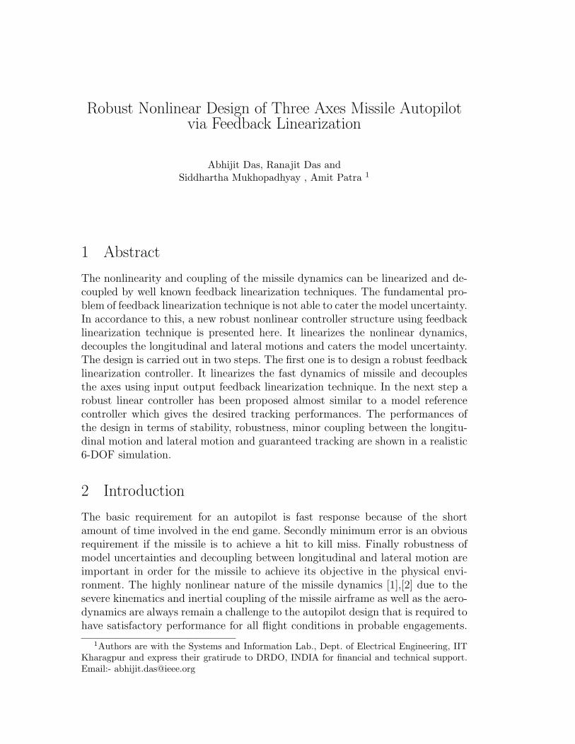
Robust Nonlinear Design of Three Axes Missile Autopilot via Feedback Linearization Abhijit Das, Ranajit Das and Siddhartha Mukhopadhyay , Amit Patra 1 1 Abstract The nonlinearity and coupling of the missile dynamics can be linearized and de- coupled by well known feedback linearization techniques. The fundamental pro- blem of feedback linearization technique is not able to cater the model uncertainty. In accordance to this, a new robust nonlinear controller structure using feedback linearization technique is presented here. It linearizes the nonlinear dynamics, decouples the longitudinal and lateral motions and caters the model uncertainty. The design is carried out in two steps. The first one is to design a robust feedback linearization controller. It linearizes the fast dynamics of missile and decouples the axes using input output feedback linearization technique. In the next step a robust linear controller has been proposed almost similar to a model reference controller which gives the desired tracking performances. The performances of the design in terms of stability, robustness, minor coupling between the longitu- dinal motion and lateral motion and guaranteed tracking are shown in a realistic 6-DOF simulation. 2 Introduction The basic requirement for an autopilot is fast response because of the short amount of time involved in the end game. Secondly minimum error is an obvious requirement if the missile is to achieve a hit to kill miss. Finally robustness of model uncertainties and decoupling between longitudinal and lateral motion are important in order for the missile to achieve its objective in the physical envi- ronment. The highly nonlinear nature of the missile dynamics [1],[2] due to the severe kinematics and inertial coupling of the missile airframe as well as the aero- dynamics are always remain a challenge to the autopilot design that is required to have satisfactory performance for all flight conditions in probable engagements. 1 Authors are with the Systems and Information Lab., Dept. of Electrical Engineering, IIT Kharagpur and express their gratirude to DRDO, INDIA for financial and technical support. Email:- [email protected]
-
Upload
dinhkhuong -
Category
Documents
-
view
235 -
download
2
Transcript of Robust Nonlinear Design of Three Axes Missile Autopilot ... 2.pdf · Robust Nonlinear Design of...
Robust Nonlinear Design of Three Axes Missile Autopilotvia Feedback Linearization
Abhijit Das, Ranajit Das andSiddhartha Mukhopadhyay , Amit Patra 1
1 Abstract
The nonlinearity and coupling of the missile dynamics can be linearized and de-coupled by well known feedback linearization techniques. The fundamental pro-blem of feedback linearization technique is not able to cater the model uncertainty.In accordance to this, a new robust nonlinear controller structure using feedbacklinearization technique is presented here. It linearizes the nonlinear dynamics,decouples the longitudinal and lateral motions and caters the model uncertainty.The design is carried out in two steps. The first one is to design a robust feedbacklinearization controller. It linearizes the fast dynamics of missile and decouplesthe axes using input output feedback linearization technique. In the next step arobust linear controller has been proposed almost similar to a model referencecontroller which gives the desired tracking performances. The performances ofthe design in terms of stability, robustness, minor coupling between the longitu-dinal motion and lateral motion and guaranteed tracking are shown in a realistic6-DOF simulation.
2 Introduction
The basic requirement for an autopilot is fast response because of the shortamount of time involved in the end game. Secondly minimum error is an obviousrequirement if the missile is to achieve a hit to kill miss. Finally robustness ofmodel uncertainties and decoupling between longitudinal and lateral motion areimportant in order for the missile to achieve its objective in the physical envi-ronment. The highly nonlinear nature of the missile dynamics [1],[2] due to thesevere kinematics and inertial coupling of the missile airframe as well as the aero-dynamics are always remain a challenge to the autopilot design that is required tohave satisfactory performance for all flight conditions in probable engagements.
1Authors are with the Systems and Information Lab., Dept. of Electrical Engineering, IITKharagpur and express their gratirude to DRDO, INDIA for financial and technical support.Email:- [email protected]

Classically, missile autopilots are designed using linear control approaches. Tra-ditional approach is to first linearize the missile short period dynamics for eachaxis about an operating condition, and then to apply linear control theory tosynthesize a feedback controller. This process is repeated at multiple operatingconditions and the controllers are then scheduled with respect to the flight con-ditions. The assumptions hold insignificant at high angle of attack because oflack of knowledge in huge model i.e. aerodynamic parameter uncertainties andcoupling. Aerodynamic considerations such as high maneuverability is must tointercept the modern threat profiles. Severe coupling due to high unwanted rolldisturbance torque at high angle of attack is the most concern in homing headmissile in view of:
1. May cause track loss of the missile homing head as seeker is having limitedgimbal freedom from physical considerations.
2. High side force disturbance may lead to control saturation of the actuationservo system.
A natural idea for handling the nonlinear dynamics is to design the autopilot onthe basis of the more accurate nonlinear model, thus leading to nonlinear autopi-lots. One of such strategies is well known feedback linearization approach whichuses the feedback and or coordinates transform to linearize the nonlinear system.Then it addresses the design issues on the linearized system thus obtained. Back-ground on the application of feedback linearization technique to missile autopilotproblem can be found in References. [3],[4] present a three axe missile autopi-lot design using classical linear time invariant control and static and dynamicapproximate input output linearizing feedback control. [5] examined the closedloop stability of an air to air missile with a dynamic inversion controller using atwo timescale separation. [6],[7] and [8] presented the linearizing transformationtechnique to the autopilot design of air to air missile systems. [9] investigatesthe feasibilities of autopilot design for highly maneuverable bank to turn mis-sile using feedback linearization based approach. All these paper works showthe comparable performances for well known model. But model uncertainty is achallenge. In the approach of the research, the nonlinear controller is designedcorresponds to a basic application of linearizing techniques combined with inputoutput linearization and time scale separation. The fast dynamics (inner loop)are linearized based on the input- output feedback linearization of the missiledynamics eventually the slow dynamics (outer loop) is designed in order to berobust with regards to uncertainties. The main feature of the research is the con-sideration of a three-axis time variant nonlinear missile model. The aerodynamicparameters are used into a look up table and as a function of mach no, angle ofattack and maneuver plane roll orientation. Sensors and actuators modeling withphysical limit are also taken into account. The objective of the present research isto design a three axes nonlinear autopilot that decoupled the roll pitch and yaw
2

axis and cater significant model uncertainties. At the same time, the autopilotperformances in terms of BW, rise time and damping are satisfactory.
3 Plant Dynamics
The nonlinear differential equations for the missile model are given as [1],[2],{u=rv−qw+ 1
m[TX−QSCDO]+gx
v=pw−ru+ 1m
[TY +QS{CS−ClςδY + D2VM
(−Cyβ β−Cyrr)}]+gy
w=wu−pv+ 1m
[Tz+QS{CN−ClηδP + D2VM
(−Czqq−Czαα)}]+gz
(1)
{p= 1
IXX[−IXXp+TMX+QSD{ D
2VMCLP p−ClξδR+Cl}]
q= 1IY Y
[−IY Y q+TMY −(IXX−IY Y )pr+QSD{−CmηδP +Cmp+ D2VM
(Cmqq+Cmαα)}]
r= 1Izz
[−Izzr+TMZ−(IY Y −IXX)pq+QSD{CmςδY +Cny+ D2VM
(Cnrr−Cmβ β)}](2)
Where, the aerodynamic coefficients are used in terms of look up table and the no-menclatures are given as: CD0 = axial force or drag coefficient, CN = Normal For-ce Coefficient, Cmp = Pitching Moment Coefficient, CS = Side Force Coefficientand CL = Rolling Moment Coefficient. All are used as a function of f (M, αR, φa).Here, αR = Resultant angle of attack and φa = Maneuver plane roll orientation.The control force and moment effectiveness are function of Mach number andcontrol deflection δ and used as a lookup table. CLξ = Roll control moment effec-tiveness, CLη and CLζ are Pitch and Yaw control force effectiveness respectively.
And moment coefficients Cmς = −CLς(Xcpδ−Xcg)
Dand Cmη = CLη
(Xcpδ−Xcg)
D. Let the
state, output and the input vectors be defined as X =[
u v w p q r]T
,
Y =[
p q r]T
and U =[
δR δP δY
]TThe plant model can be represented
asX = f (X) + g (X) U
Y = h(X)(3)
Where,
f (X) =
f1
f2
f2
f4
f5
f6
=
rv − qw + 1m
[TX −QSCDO] + gx
pw − ru + 1m
[TY + QS{CS + D2VM
(−Cyββ − Cyrr)}] + gy
wu− pv + 1m
[Tz + QS{CN + D2VM
(−Czqq − Czαα)}] + gz1
IXX[−IXXp + TMX + QSD{ D
2VMCLP p + Cl}]
1IY Y
[−IY Y q + TMY − (IXX − IY Y )pr + QSD{Cmp + D2VM
(Cmqq + Cmαα)}]1
Izz[−Izzr + TMZ − (IY Y − IXX)pq + QSD{Cny + D
2VM(Cnrr − Cmββ)}]
3

and
g (X) =
0 0 0
0 0 QSClς/m0 −QSClη/m 0
−QSDClξ/IXX0 0
0 −QSDCmη/IY Y0
0 0 QSDCmς/IZZ
3.1 Application of feedback linearization
The central idea of the feedback linearization is to algebraically transform a non-linear system dynamics into a linear form by using state feedback, with inputstate linearization corresponding to complete linearization and input output li-nearization to partial linearization. The theory is well known and available intext books [10],[11]. Here the design methodology is presented only. The systemunder consideration is described by
X(t) = f(X(t)) + g(X(t))U(t)
Y (t) = h(X(t))(4)
Where, X(t) is the n−dimensional plant state, U(t) is m−dimensional plantinput and Y (t) is m−dimensional plant output. f : Rn → Rn, g : Rn → Rn×Rm
is m− and h : Rn → Rm are smooth functions. The input output feedbacklinearization of 3.1 can be performed if there exist constants ρ1, ρ2, ....., ρm andinput output mapping of the form
y(ρ1)1 (t)
y(ρ2)2 (t)
.
.
y(ρm)m (t)
= B (X (t)) + A (X (t))
u1 (t)u2 (t)
.
.um (t)
(5)
Where, ui, yi, i = 1, ...,m are components of U and Y , B : Rn → Rm and A :Rn → Rm × Rm are smooth with A(X(t)) invertible. For if this is the case, thefollowing feedback control
U (t) = A−1 (X (t)) [V (t)−B (X (t))] (6)
Where, V (t) =[
V1 (t) V2 (t) . . Vm (t)]T ∈ Rm yields
y(ρi)i (t) = Vi (t) , i = 1, 2, ...,m (7)
Since the new input Vi only affects the output Yi, (3.1) is called a decouplingcontrol law and the invertible matrix A(X) is called the decoupling matrix of thesystem. On the basis of it, single input, single output linear control techniquescan be utilized to achieve the desired objectives.
4
3.1.1 Design formulation
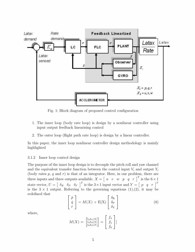
The design is carried out using a two time scale assumption to separate thedynamics as shown in Fig.1.
Fig. 1: Block diagram of proposed control configuration
1. The inner loop (body rate loop) is design by a nonlinear controller usinginput output feedback linearising control
2. The outer loop (flight path rate loop) is design by a linear controller.
In this paper, the inner loop nonlinear controller design methodology is mainlyhighlighted
3.1.2 Inner loop control design
The purpose of the inner loop design is to decouple the pitch roll and yaw channeland the equivalent transfer function between the control input Vi and output Yi
(body rates p, q and r) is that of an integrator. Here, in our problem, there are
three inputs and three outputs available. X =[
u v w p q r]T
is the 6×1
state vector, U =[
δR δP δY
]Tis the 3×1 input vector and Y =
[p q r
]T
is the 3 × 1 output. Referring to the governing equations (1),(2), it may beredefined that p
qr
= M(X) + E(X)
δR
δP
δY
(8)
where,
M(X) =
[Lfh1(X)Lfh2(X)Lfh3(X)
]=
f4
f5
f6
]
5

and the decoupling matrix
E(X) =
Lg1h1 Lg2
h1 Lg3h1
Lg1h2 Lg2
h2 Lg3h2
Lg1h3 Lg2
h3 Lg3h3
=
−QSDClξ/IXX0 0
0 −QSDCmη/IY Y0
0 0 QSDCmς/IZZ
The 3×3 matrix E(X) is invertible over the region. Then the input transformation[12],[13].
U =
δR
δP
δY
= E−1
v1 − Lr1f h1
v2 − Lr2f h2
v3 − Lr3f h3
or δR
δP
δY
= −E−1M + E−1[
v1v2v3
](9)
The above three equations of the simple form[
p q r]T
=[
v1 v2 v3
]T.
Hence the control law decouples the longitudinal motion and lateral motion. Inpractice, the system description is rarely known exactly. The model uncertaintyis not able to cater by the feedback linearization control law as shown in 9. Thefeedback linearization can only be performed based on nominal plant. Now ourobjective is how to control the plant uncertainty. After a lot of literature survey, itis found that various robust schemes have been proposed to account for the modeluncertainty for the state input linearizable system and input output linearizablesystem. Basically after feedback linearized plant, a robust controller is designedto handle the plant uncertainty. In this research, a robust feedback linearizationscheme based on model reference adaptive control is proposed to cater the modeluncertainty. The scheme shows significant performances and this is one of themain contributions of this research. The derivation of the scheme is presented inthe following section. The robustness of the scheme will be presented through alot of 6−DOF simulation.
3.2 Robust feedback linearization control
For simplicity, let we denote the nominal plant (model) output is YN and actualplant output is Y . The output equation may be expressed as
Y = M (X) + E (X) U
YN = MN (XN) + EN (XN) U(10)
The model uncertainty is included in M(X) and E(X). The input output re-lationship of the nominal plant as discussed earlier is YN = VN , where therelationship between the linear control VN and the plant input U is given byU = E−1
N [VN −MN ]. Our objective is to derive a new linear control V and the
6

relationship between this new input V to FBLC and actual plant input U suchthat it will linearize and decouple the output equation in the form Y = V . Nowdoing some mathematical formulation, we can express V in terms of VN and aswell as in terms of U as follows
V − VN = Y − YN ⇒ VN = V −(Y − YN
)(11)
Hence, the control input is obtained as
U = E−1N
[V −
(Y − YN
)−MN
](12)
The inner loop block diagram with robust feedback linearization control law isshown in Fig.2. The same input signal U goes to model as well as plant. The actual
output is compared with the expected output and the error signal(Y − YN
)is
feedback to the reference input V . Hence, the equivalent transfer function betweenthe input signal V and the actual output Y is just like an integrator. It may benoted that under perturbed cases also, the robust scheme holds the linearity anddecoupling properties.
Fig. 2: Modified robust feedback linearization controller
The inner loop of the dynamic inversion control law controls the fast states p,q and r. This loop calculates the virtual control surface deflection commands[
v1 v2 v3
]from the rate commands given
[pd qq rd
]by the slow dyna-
mics[
φ fz fy
]. The desired dynamics used are given by p = k4 (pd − p) , q =
k5 (qd − q) and r = k6 (rd − r) , where k4, k5 and k6 are design parameters. Hencemay be written that v1
v2
v3
=
k4 (pd − p)k5 (qd − q)k6 (rd − r)
(13)
7

3.3 Outer loop design
Here the basic assumption is that the coupling between the force and controldeflections is relative small in comparison with the coupling between the momentand control deflection [1]. Hence, it is neglected. The linearized plant transferfunctions between rate and latax are derived as
fz
q=−Vm
(1− s2
ω2z
)(1 + Tαs)
,fy
r=
Vm
(1− s2
ω2z
)(1 + Tαs)
andφ
p=
1
s
The gains k1, k2, k3 are designed to satisfy the desired specifications of autopilotas demanded by the guidance loop.
4 Simulation results
The design is thoroughly validated in a full scale 6−DOF platform consideringall the plant parameter variations. A conventional linear three loop lateral auto-pilot and a PI type roll autopilot are also designed to show the potential of thenonlinear autopilot performance as a comparison. All the cases, the nominal aswell as off nominal cases, the performances of the nonlinear autopilot are carriedout in two stages.
1. Performances of the nonlinear autopilot by applying step body rate deman-ds (inner loop performances).
2. Performance of the nonlinear autopilot by applying step latax demands(outer loop performances).
The performances are compared with linear controller and discussed in the follo-wing section.
4.1 Autopilot performances by applying step body rate demands
In 6-DOF, body rate is forced and are applied to inner loop as demand for differenttime intervals for different channels. Fig.3 shows that body rate response of thenonlinear controller for nominal condition when the pitch body rate is demandedat 10.5 sec, yaw rate is demanded at 12.3 sec and roll rate is demanded at 11.3sec. It may be pointed out from the Figure that the ignition of body rate in onechannel is not affects the other two channels. It proves the evidence of decoupling.The autopilot response is almost critically damped in nature and time constant(0.05 sec) indicates the band width of the order of 4Hz. It again validates thelinear controller design. Fig.4 shows the same with disturbance condition andcompared with the performances obtained with conventional linear controller.Here also it may found that the nonlinear controller decouples the longitudinal
8

Fig. 3: Body rate profiles with forced body rate demand
Fig. 4: A comparative performances with forced body rate demand
and lateral motion. Where, linear controller fails to decouple the motions. We
9

may note from Fig.4 that severe coupling for linear controller when simultaneouspitch and yaw maneuver is present.
4.2 Autopilot performances by applying step latax demands
Latax demand is forced as a outer loop demand for pitch and yaw channel,whereas, roll channel demand is zero. A step Pitch latax demand of 40m/s2is applied at 10.5 sec where as, a step yaw latax demand of 5m/s2 is appliedat 12.3 sec. The corresponding latax profiles are shown in Fig.5 The body rate
Fig. 5: Autopilot Performances for step latax demand
profiles are shown in Fig.6. Here, also significant amount of decoupling amongthe three axes may be found compared to linear controller. The roll rate is almostsilent for the nonlinear controller which is the main objective of the design. Thecontrol deflection profiles are shown in Fig.7.
5 Conclusion
This paper demonstrates the design of a nonlinear controller using feedback linea-rization technique for the missile control problem associated with severe couplingof longitudinal and lateral motion and significant plant uncertainty. The nonline-ar autopilot design methodology is carried out in two time scale separation. The
10

Fig. 6: Body rate profiles for step latax demand
Fig. 7: Control deflection for step latax demand
11

design is validated here through a full scale 6−DOF simulation. A comparison isalso made with linear traditional controller. Comparing the 6−DOF simulationresults, the following salient features of the new nonlinear controller design maybe noted:
1. It decouples the roll, pitch and yaw channel.
2. The roll rate is fairly close to zero during maneuver phases. The FBLCreduces the roll induced yaw rate and control requirement and hence controlsaturation.
3. The autopilot response (both latax as well as body rate) is significantlyfaster. Quick correction is possible.
REFERENCES
[1] P. Garnell and D. J. East, Guided Weapon Control System. PergamonPress,2nd Ed.,Oxford, 1980.
[2] A. L. Greensite, Analysis and Design of Space Vehicle Flight Control Sy-stems. Pergamon Press,2nd Ed.,Oxford, 1970.
[3] E. Devaud, J.-P. Harcaut, and H. Siguerdidjane, “Three-axes missile autopi-lot design: From linear to nonlinear control strategies,” Journal of Guidance,Control, and Dynamics, vol. 24, no. 1, pp. 64–71, January-February 2001.
[4] ——, “Various strategies to design a three axes missile autopilot,” AIAA,no. 3976, 1999.
[5] C. Schumacher and P. Khargonekar, “Stability analysis of a missile controlsystem with a dynamic inversion controller,” Journal of Guidance, Controland Dynamics, vol. 21, June 1998.
[6] M. Tahk, M. M. Brigges, and P. Menon, “Application of plant inversionvia state feedback to missile autopilot design,” Procedings of the 27th IEEEConference on Decesion and Control, pp. 730–735, December 1988.
[7] P. Menon and M. Yousefpor, “Design of nonlinear autopilots for high angleof attack missiles,” Optimal Synthesis, 1996.
[8] P. Menon, V. Iragavarapu, and E. Ohlmeyer, “Nonlinear missile autopilotusing time scale separation,” AIAA, vol. 96-3765, 1997.
[9] J. Huang, C. F. Lin, J. R. Cloutier, J. H. Evers, and C. D. Souza, “Ro-bust feedback linearization approach to autopilot design,” Proc. IEEE Conf.Contr. Applicat., vol. 1, pp. 220–225, 1992.
12

[10] J.-J. E. Slotine and W. Li, Applied Nonlinear Control. Prentice Hall, 1991.
[11] A. Isidori, Nonlinear Control Systems: an introduction. Berlin: Springer-Verlag, 1989.
[12] A. Das, R. Das, S. Mukhopadhyay, and A. Patra, “Nonlinear autopilot andobserver design for a surface-to-surface, skid-to-turn missile,” Second Indiaannual conference, Proceedings of the IEEE INDICON 2005, pp. 304 – 308,11-13 December 2005.
[13] ——, “Sliding mode controller along with feedback linearization for a nonli-near missile model,” 1st International Symposium on Systems and Controlin Aerospace and Astronautics, 19-21 January 2006.
13