Robust Network Compressive Sensing Lili Qiu UT Austin NSF Workshop Nov. 12, 2014.
24
Robust Network Compressive Sensing Lili Qiu UT Austin NSF Workshop Nov. 12, 2014
-
Upload
dwain-singleton -
Category
Documents
-
view
220 -
download
0
Transcript of Robust Network Compressive Sensing Lili Qiu UT Austin NSF Workshop Nov. 12, 2014.

Robust Network Compressive Sensing
Lili QiuUT Austin
NSF WorkshopNov. 12, 2014

Network Matrices and Applications
• Network matrices– Traffic matrix– Loss matrix– Delay matrix– Channel State Information (CSI) matrix– RSS matrix
2
3
Q: How to fill in missing values in a matrix?
1
3
2router
flow 1
flow 3
flow 2
link 2link 1
link 3
flow 1
flow 2
flow 3
time 1 time 2 …
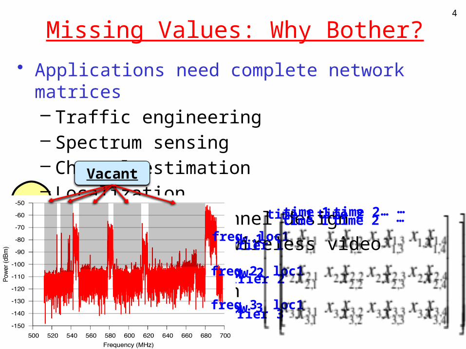
• Applications need complete network matrices– Traffic engineering– Spectrum sensing– Channel estimation– Localization– Multi-access channel design– Network coding, wireless video coding– Anomaly detection– Data aggregation– …
Missing Values: Why Bother?4
subcarrier 1
subcarrier 2
subcarrier 3
time 1 time 2 …
Vacant
freq ,loc1
freq 2, loc1
freq 3, loc1
time 1 time 2 …
5
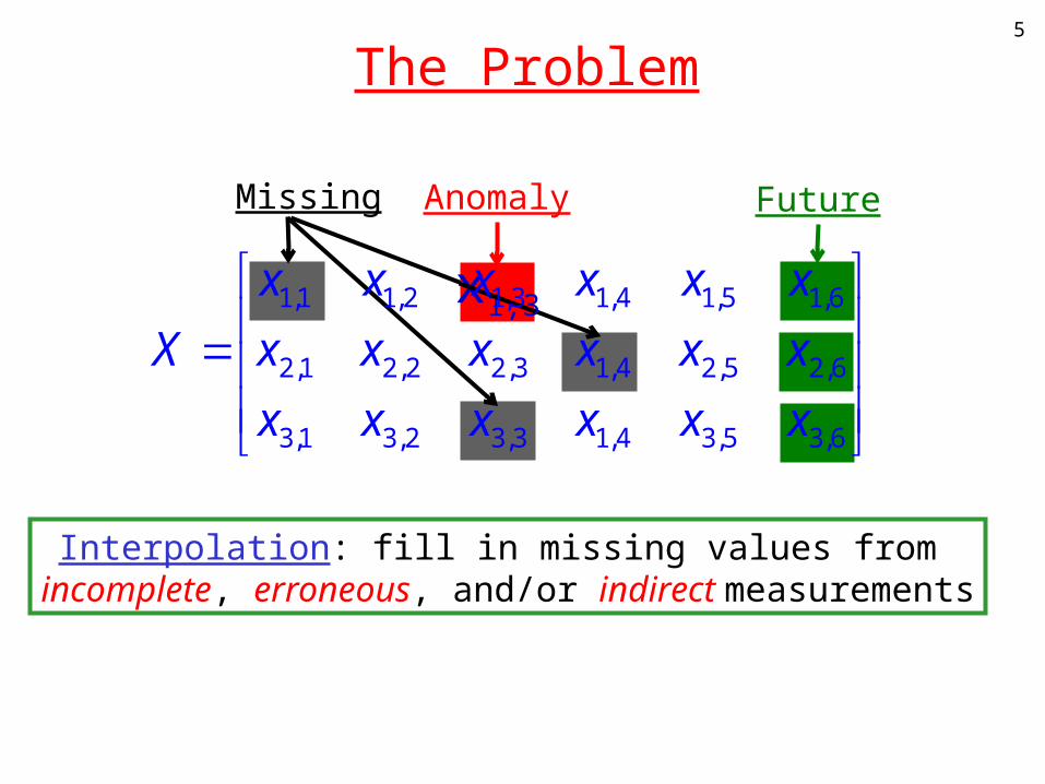
The Problem
6,3
6,2
6,1
5,3
5,2
5,1
4,13,32,3
4,13,22,2
4,13,12,1
1,3
1,2
1,1
x
x
x
x
x
x
xxx
xxx
xxx
x
x
x
X
Interpolation: fill in missing values from incomplete, erroneous, and/or indirect measurements
Anomaly FutureMissing
x1,3
State of the Art
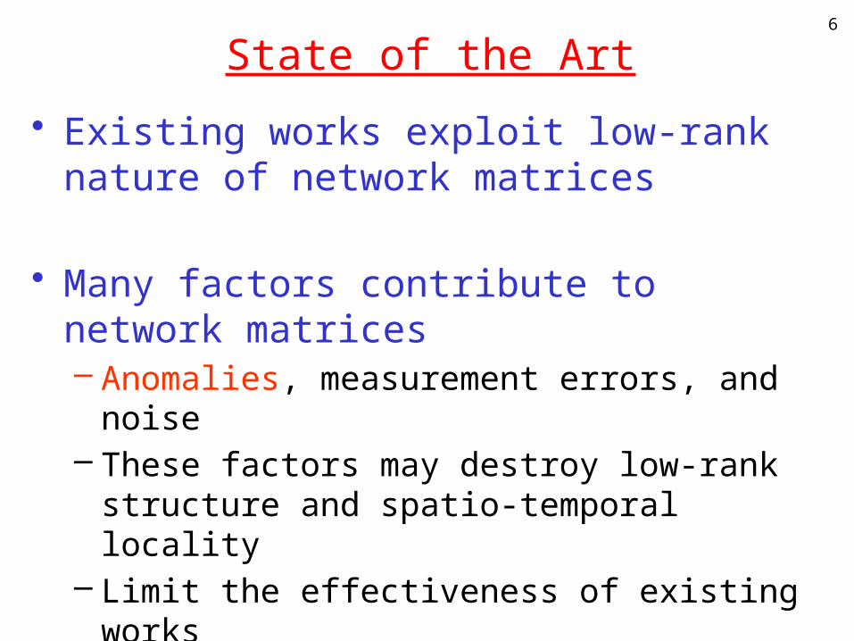
• Existing works exploit low-rank nature of network matrices
• Many factors contribute to network matrices– Anomalies, measurement errors, and noise– These factors may destroy low-rank
structure and spatio-temporal locality– Limit the effectiveness of existing works
6

Network Matrices
Network Date Duration Size (flows/links x #timeslot)
3G traffic 11/2010 1 day 472 x 144
WiFi traffic 1/2013 1 day 50 x 118
Abilene traffic 4/2003 1 week 121 x 1008
GEANT traffic 4/2005 1 week 529 x 672
1 channel CSI 2/2009 15 min. 90 x 9000
Multi. Channel CSI
2/2014 15 min. 270 x 5000
Cister RSSI 11/2010 4 hours 16 x 10000
CU RSSI 8/2007 500 frames 895 x 500
Umich RSS 4/2006 30 min. 182 x 3127
UCSB Meshnet 4/2006 3 days 425 x 1527
7
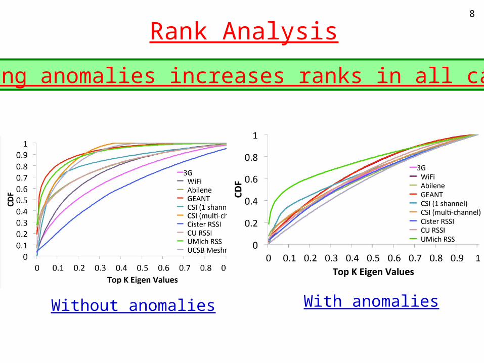
Rank Analysis8
Adding anomalies increases ranks in all cases.
Without anomalies With anomalies
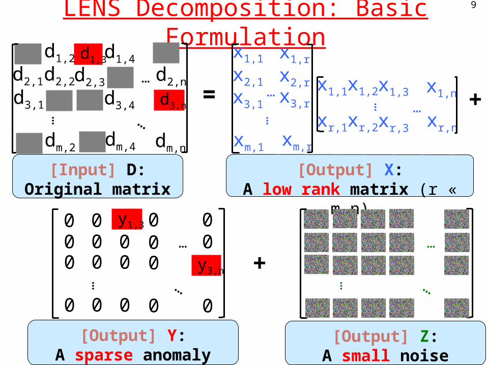
LENS Decomposition: Basic Formulation
9
= +
y1,30…
…
…y3,n
0 0 0000 00000 0
000 0 0
+
[Input] D:Original matrix
[Output] X:A low rank matrix (r «
m,n)
[Output] Y:A sparse anomaly
matrix
[Output] Z:A small noise
matrix
d1,3d1,2
…
…
…
d2,n
dm,n
d3,n
d1,4
d2,1 d2,2 d2,3
d3,1 d3,4
dm,2 dm,4
…
xm,r
xr,n
…
x1,1
x2,1
x3,1
xm,1
x3,r
x2,r
x1,r
x1,1
xr,1 xr,2
x1,2
xr,3
x1,3 x1,n… …
…
…
…

LENS Decomposition: Basic Formulation
• Formulate it as a convex opt. problem:
10
min:
subject to:
= + +d1,3
d1,2 d1,4
[Input] D:Original matrix
x1,2 x1,4
[Output] X:A low rank
matrix
0 0 y1,3 0
0 0 0 0
0 0 0 0
[Output] Y:A sparse anomaly matrix
[Output] Z:A small noise
matrix
α βσ
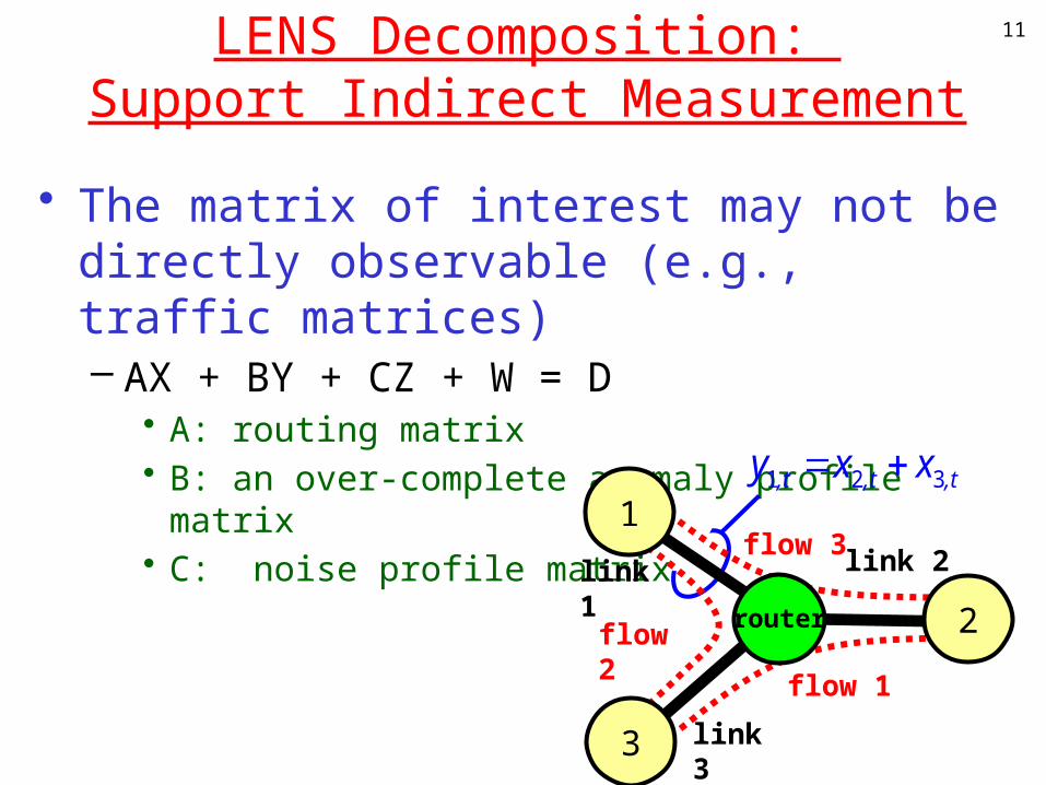
LENS Decomposition: Support Indirect Measurement
• The matrix of interest may not be directly observable (e.g., traffic matrices)– AX + BY + CZ + W = D
• A: routing matrix• B: an over-complete anomaly profile matrix• C: noise profile matrix
11
,t,t,t xxy 321 1
3
2router
flow 1
flow 3
flow 2
link 2link 1
link 3

LENS Decomposition: Account for Domain Knowledge
• Domain Knowledge– Temporal stability– Spatial locality– Initial solution
12
min:
subject to:
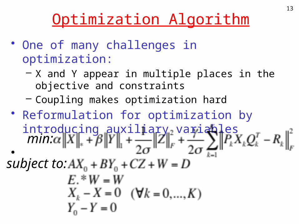
Optimization Algorithm
• One of many challenges in optimization:– X and Y appear in multiple places in the objective
and constraints– Coupling makes optimization hard
• Reformulation for optimization by introducing auxiliary variables
•
13
min:
subject to:

Optimization Algorithm• Alternating Direction Method (ADM)
– For each iteration, alternate among the optimization of the augmented Lagrangian function by varying each one of X, Xk, Y, Y0, Z, W, M, Mk, N while fixing the other variables
– Improve efficiency through approximate SVD
14

Setting Parameters
• • •
where (mX,nX) is the size of X, (mY,nY) is the size of Y, η(D) is the fraction of entriesneither missing or erroneous, θ is a control parameter that limitscontamination of dense measurement noise
15
min:α βσ σ
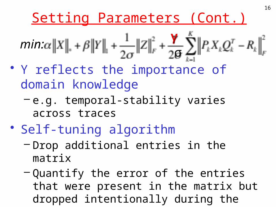
Setting Parameters (Cont.)
• ϒ reflects the importance of domain knowledge– e.g. temporal-stability varies across traces
• Self-tuning algorithm– Drop additional entries in the matrix– Quantify the error of the entries that were
present in the matrix but dropped intentionally during the search
– Pick ϒ that gives lowest error
16
min:σ
γ

17
Algorithms Compared
Algorithm Description
Baseline Baseline estimate via rank-2 approximation
SVD-base SRSVD with baseline removal
SVD-base +KNN Apply KNN after SVD-base
SRMF [SIGCOMM09] Sparsity Regularized Matrix Factorization
SRMF+KNN [SIGCOMM09]
Hybrid of SRMF and KNN
LENS Robust network compressive sensing
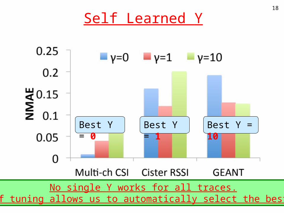
Self Learned ϒ18
Best ϒ = 0 Best ϒ = 1 Best ϒ = 10
No single ϒ works for all traces.Self tuning allows us to automatically select the best ϒ.

Interpolation under anomalies19
CU RSSI
LENS performs the best under anomalies.

Interpolation without anomalies20
CU RSSI
LENS performs the best even without anomalies.

Conclusion
• Main contributions– Important impact of anomalies in matrix
interpolation– Decompose a matrix into
• a low-rank matrix, • a sparse anomaly matrix, • a dense but small noise matrix
– An efficient optimization algorithm– A self-learning algorithm to automatically tune the
parameters• Future work
– Applying it to spectrum sensing, channel estimation, localization, etc.
21

22
Thank you!

Evaluation Methodology
• Metric– Normalized Mean Absolute Error for missing values
• Report the average of 10 random runs• Anomaly generation
– Inject anomalies to a varying fraction of entries with varying sizes
• Different dropping models
23

Summary of Other Results
• The improvement of LENS increases with anomaly sizes and # anomalies.
• LENS consistently performs the best under different dropping modes.
• LENS yields the lowest prediction error.
• LENS achieves higher anomaly detection accuracy.
24