Robust Navigation In GNSS DegradedEnvironment Using Graph Optimization

Ryan M. Watson and Jason N. Gross , West Virginia University

BiographyMr. Ryan M. Watson is a Graduate Research Assistant within the Navigation Laboratory in the Department of Mechanicaland Aerospace (MAE) Engineering at WVU and is pursuing his PhD in aerospace engineering. He completed his Master inaerospace engineering at WVU in 2017, with a thesis on the integration of Inertial Navigation in JPL’s RTGx Precise PointPositioning software. Mr. Watson earned his B.S. degree in mechanical engineering from WVU in 2014.

Dr. Jason N. Gross is an assistant professor at West Virginia University (WVU) were he directs WVU’s Navigation Laboratory.He received his Ph.D. in aerospace engineering from WVU in 2011 and the worked at the Jet Propulsion Laboratory (JPL) untilJanuary 2014. His research is focused on Guidance, Navigation & Control (GNC) technologies and he currently serves as anassociate member of the AIAA’s GNC technical committee. He is a member of the ION, the AIAA, and the IEEE.

AbstractRobust navigation in urban environments has received a considerable amount of both academic and commercial interest overrecent years. This is primarily due to large commercial organizations such as Google and Uber stepping into the autonomousnavigation market. Most of this research has shied away from Global Navigation Satellite System (GNSS) based navigation.The aversion to utilizing GNSS data is due to the degraded nature of the data in urban environment (e.g., multipath, poor satellitevisibility). The degradation of the GNSS data in urban environments makes it such that traditional (GNSS) positioning methods( e.g., extended Kalman filter, particle filters) perform poorly. However, recent advances in robust graph theoretic based sensorfusion methods, primarily applied to Simultaneous Localization and Mapping (SLAM) based robotic applications, can also beapplied to GNSS data processing. This paper will utilize one such method known as Incremental Smoothing and Mapping(ISAM2) in conjunction several robust optimization techniques to evaluate their applicability to robust GNSS data processing.The goals of this study are two-fold. First, for GNSS applications, we will experimentally evaluate the effectiveness of robustoptimization techniques within a graph theoretic estimation framework. Second, by releasing the software developed and datasets used for this study, we will introduce a new open-source front-end to the Georgia Tech Smoothing and Mapping (GTSAM)library for the purpose of integrating GNSS pseudorange observations.

IntroductionTraditionally, GNSS data is not utilized to its full potential for autonomously navigating vehicles in urban environments. This islargely ascribable to the possibility of GNSS observables be degraded (e.g., multipath, poor satellite geometry) when confrontedwith an urban environment. However, the inclusion of GNSS data in such systems would provide substantial information totheir navigation algorithms. So, the ability to safely incorporate GNSS observables into existing inference algorithms, evenwhen confronted with environments that have the potential to degrade GNSS observables, is of obvious importance.

To overcome the aforementioned issues, we will leverage the advances made within the robotics community surround-ing graph-based simultaneous localization and mapping (SLAM) to efficiently and robustly process GNSS data. Within thiscommunity, the advances surrounding optimization have been made on two fronts: optimization speed and robustness. Forprocessing speed, the incremental smoothing and mapping (ISAM2) (Kaess et al., 2012) algorithm provides a real-time op-timization routine (Whelan et al., 2015) and, as such, will be utilized as the optimization framework for this study. Forrobust graph optimization, the literature can be divided into two broad subsets: traditional M-Estimators (Huber, 1981), andmore recent graph based robust methods (Sunderhauf and Protzel, 2012), (Agarwal et al., 2013), (Olson and Agarwal, 2012).

This paper will evaluate the effectiveness of the mentioned robust optimization techniques when applied specifically to GNSSpseudorange data processing.

The remainder of this paper is organized as follows. First, the technical approach utilized for this study is described, whichbegins with a discussion on factor graph optimization and then evolves into a discussion on how to make that optimization morerobust to erroneous data. Next, the experiential setup and collected data sets are discussed. Then, the results obtained using thepreviously described models and data sets are provided. Finally, the paper ends with concluding remarks and proposed stepsfor continued research.

1 Technical ApproachThis section provides concise overview of the sensor fusion approach utilized in this study. For the reasons mentioned above,it was decided to use a graph-theoretic approach for sensor fusion as opposed to the more common Kalman (Kalman, 1960) orparticle filters (Thrun, 2002). To describe our approach, first, the factor graph (Kschischang and Frey, 2001) is discussed. Then,the evolution from the factor graph to Incremental Smoothing and Mapping (ISAM2) (Kaess et al., 2012) is covered. Next,a discussion is provided on the incorporation of GNSS pseudorange observables into the factor graph framework. Finally, adiscussion is provided on methods to make these graph theoretic approaches more tolerant to measurement faults, specifically,in the context of GNSS.

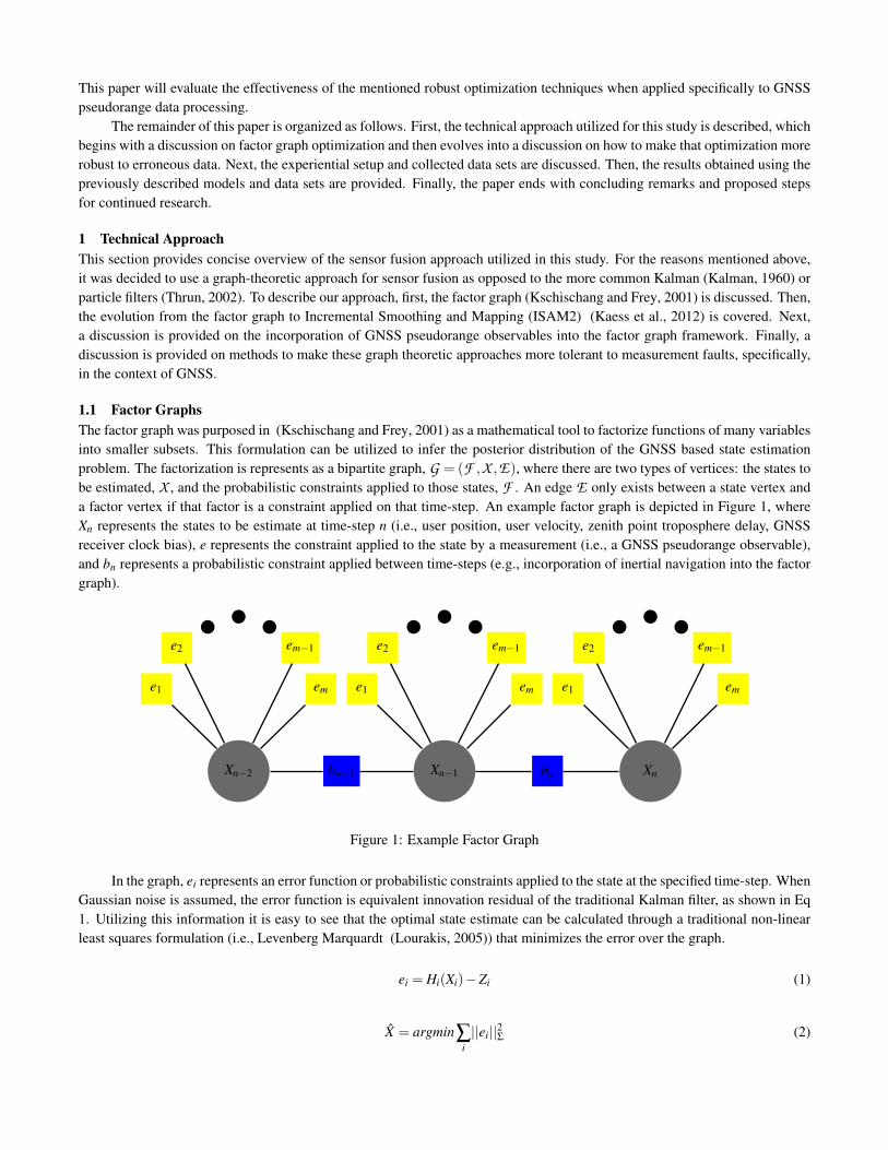
1.1 Factor GraphsThe factor graph was purposed in (Kschischang and Frey, 2001) as a mathematical tool to factorize functions of many variablesinto smaller subsets. This formulation can be utilized to infer the posterior distribution of the GNSS based state estimationproblem. The factorization is represents as a bipartite graph, G = (F ,X ,E), where there are two types of vertices: the states tobe estimated, X , and the probabilistic constraints applied to those states, F . An edge E only exists between a state vertex anda factor vertex if that factor is a constraint applied on that time-step. An example factor graph is depicted in Figure 1, whereXn represents the states to be estimate at time-step n (i.e., user position, user velocity, zenith point troposphere delay, GNSSreceiver clock bias), e represents the constraint applied to the state by a measurement (i.e., a GNSS pseudorange observable),and bn represents a probabilistic constraint applied between time-steps (e.g., incorporation of inertial navigation into the factorgraph).

Xn−2 Xn−1 Xn

e1

e2 em−1

em

bn−1

e1

e2 em−1

em

bn

e1

e2 em−1

em

Figure 1: Example Factor Graph

In the graph, ei represents an error function or probabilistic constraints applied to the state at the specified time-step. WhenGaussian noise is assumed, the error function is equivalent innovation residual of the traditional Kalman filter, as shown in Eq1. Utilizing this information it is easy to see that the optimal state estimate can be calculated through a traditional non-linearleast squares formulation (i.e., Levenberg Marquardt (Lourakis, 2005)) that minimizes the error over the graph.

ei = Hi(Xi)−Zi (1)

X = argmin∑i||ei||2Σ (2)

1.1.1 Incremental Smoothing and Mapping

The factor graph works great when post-processing data; however, it is a batch estimator and cannot effectively operate inreal-time when sufficiently large amounts of data have been incorporated into the graph (Indelmana et al., 2013). To overcomethis limitation, the Incremental Smoothing and Mapping formulation was developed (Kaess et al., 2012). This formulationmoves from an un-directed graphical structure known as the Bayes tree (Kaess et al., 2010). The additional informationincorporated into the graph allows the optimizer to re-linearize only the vertices that are affected by the incorporation of thenew measurement to the graph (e.g., most of the graph is left unchanged when a new pseudorange observable is incorporated).

1.1.2 Pseudorange Factor

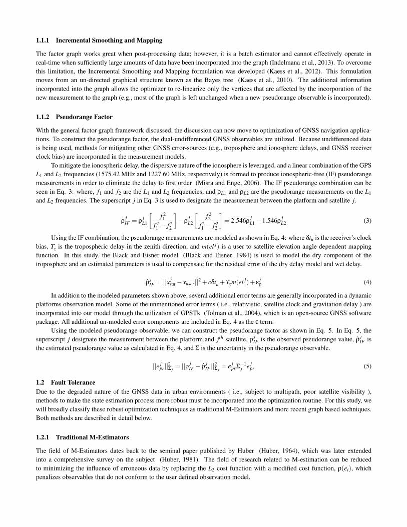
With the general factor graph framework discussed, the discussion can now move to optimization of GNSS navigation applica-tions. To construct the pseudorange factor, the dual-undifferenced GNSS observables are utilized. Because undifferenced datais being used, methods for mitigating other GNSS error-sources (e.g., troposphere and ionosphere delays, and GNSS receiverclock bias) are incorporated in the measurement models.

To mitigate the ionospheric delay, the dispersive nature of the ionosphere is leveraged, and a linear combination of the GPSL1 and L2 frequencies (1575.42 MHz and 1227.60 MHz, respectively) is formed to produce ionospheric-free (IF) pseudorangemeasurements in order to eliminate the delay to first order (Misra and Enge, 2006). The IF pseudorange combination can beseen in Eq. 3: where, f1 and f2 are the L1 and L2 frequencies, and ρL1 and ρL2 are the pseudorange measurements on the L1

and L2 frequencies. The superscript j in Eq. 3 is used to designate the measurement between the platform and satellite j.

ρjIF = ρ

jL1

[f 21

f 21 − f 2

2

]−ρ

jL2

[f 22

f 21 − f 2

2

]= 2.546ρ

jL1−1.546ρ

jL2 (3)

Using the IF combination, the pseudorange measurements are modeled as shown in Eq. 4: where δtu is the receiver’s clockbias, Tz is the tropospheric delay in the zenith direction, and m(el j) is a user to satellite elevation angle dependent mappingfunction. In this study, the Black and Eisner model (Black and Eisner, 1984) is used to model the dry component of thetroposphere and an estimated parameters is used to compensate for the residual error of the dry delay model and wet delay.

ρjIF = ||x j

sat − xuser||2 + cδtu +Tzm(el j)+ εjρ (4)

In addition to the modeled parameters shown above, several additional error terms are generally incorporated in a dynamicplatforms observation model. Some of the unmentioned error terms ( i.e., relativistic, satellite clock and gravitation delay ) areincorporated into our model through the utilization of GPSTk (Tolman et al., 2004), which is an open-source GNSS softwarepackage. All additional un-modeled error components are included in Eq. 4 as the ε term.

Using the modeled pseudorange observable, we can construct the pseudorange factor as shown in Eq. 5. In Eq. 5, thesuperscript j designate the measurement between the platform and jth satellite, ρ

jIF is the observed pseudorange value, ρ

jIF is

the estimated pseudorange value as calculated in Eq. 4, and Σ is the uncertainty in the pseudorange observable.

||e jpr||2Σ j

= ||ρ jIF − ρ

jIF ||

2Σ j

= e jprΣ−1j e j

pr (5)

1.2 Fault ToleranceDue to the degraded nature of the GNSS data in urban environments ( i.e., subject to multipath, poor satellite visibility ),methods to make the state estimation process more robust must be incorporated into the optimization routine. For this study, wewill broadly classify these robust optimization techniques as traditional M-Estimators and more recent graph based techniques.Both methods are described in detail below.

1.2.1 Traditional M-Estimators

The field of M-Estimators dates back to the seminal paper published by Huber (Huber, 1964), which was later extendedinto a comprehensive survey on the subject (Huber, 1981). The field of research related to M-estimation can be reducedto minimizing the influence of erroneous data by replacing the L2 cost function with a modified cost function, ρ(ei), whichpenalizes observables that do not conform to the user defined observation model.

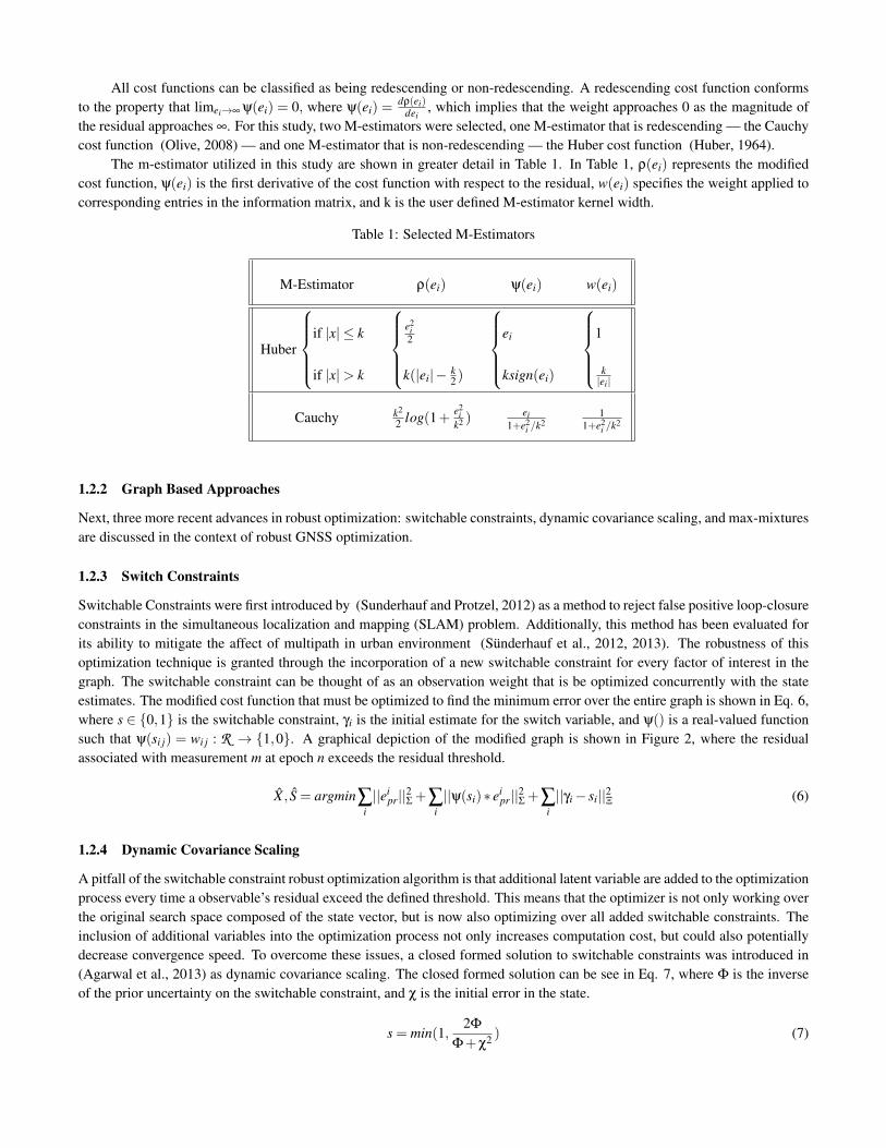
All cost functions can be classified as being redescending or non-redescending. A redescending cost function conformsto the property that limei→∞ ψ(ei) = 0, where ψ(ei) =

dρ(ei)dei

, which implies that the weight approaches 0 as the magnitude ofthe residual approaches ∞. For this study, two M-estimators were selected, one M-estimator that is redescending — the Cauchycost function (Olive, 2008) — and one M-estimator that is non-redescending — the Huber cost function (Huber, 1964).

The m-estimator utilized in this study are shown in greater detail in Table 1. In Table 1, ρ(ei) represents the modifiedcost function, ψ(ei) is the first derivative of the cost function with respect to the residual, w(ei) specifies the weight applied tocorresponding entries in the information matrix, and k is the user defined M-estimator kernel width.

Table 1: Selected M-Estimators

M-Estimator ρ(ei) ψ(ei) w(ei)

Huber

if |x| ≤ k

if |x|> k

e2

i2

k(|ei|− k2 )

ei

ksign(ei)

1

k|ei|

Cauchy k2

2 log(1+ e2i

k2 )ei

1+e2i /k2

11+e2

i /k2

1.2.2 Graph Based Approaches

Next, three more recent advances in robust optimization: switchable constraints, dynamic covariance scaling, and max-mixturesare discussed in the context of robust GNSS optimization.

1.2.3 Switch Constraints

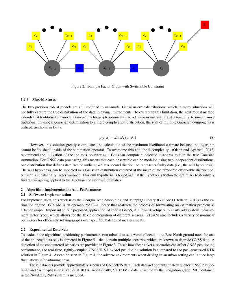
Switchable Constraints were first introduced by (Sunderhauf and Protzel, 2012) as a method to reject false positive loop-closureconstraints in the simultaneous localization and mapping (SLAM) problem. Additionally, this method has been evaluated forits ability to mitigate the affect of multipath in urban environment (Sunderhauf et al., 2012, 2013). The robustness of thisoptimization technique is granted through the incorporation of a new switchable constraint for every factor of interest in thegraph. The switchable constraint can be thought of as an observation weight that is be optimized concurrently with the stateestimates. The modified cost function that must be optimized to find the minimum error over the entire graph is shown in Eq. 6,where s ∈ {0,1} is the switchable constraint, γi is the initial estimate for the switch variable, and ψ() is a real-valued functionsuch that ψ(si j) = wi j : R → {1,0}. A graphical depiction of the modified graph is shown in Figure 2, where the residualassociated with measurement m at epoch n exceeds the residual threshold.

X , S = argmin∑i||ei

pr||2Σ +∑i||ψ(si)∗ ei

pr||2Σ +∑i||γi− si||2Ξ (6)

1.2.4 Dynamic Covariance Scaling

A pitfall of the switchable constraint robust optimization algorithm is that additional latent variable are added to the optimizationprocess every time a observable’s residual exceed the defined threshold. This means that the optimizer is not only working overthe original search space composed of the state vector, but is now also optimizing over all added switchable constraints. Theinclusion of additional variables into the optimization process not only increases computation cost, but could also potentiallydecrease convergence speed. To overcome these issues, a closed formed solution to switchable constraints was introduced in(Agarwal et al., 2013) as dynamic covariance scaling. The closed formed solution can be see in Eq. 7, where Φ is the inverseof the prior uncertainty on the switchable constraint, and χ is the initial error in the state.

s = min(1,2Φ

Φ+χ2 ) (7)

Xn−2 Xn−1 Xn

e1

e2 em−1

em

b1

e1

e2 em−1

em

b2

e1

e2 em−1

em

S1

Figure 2: Example Factor Graph with Switchable Constraint

1.2.5 Max-Mixtures

The two previous robust models are still confined to uni-modal Gaussian error distributions, which in many situations willnot fully capture the true distribution of the data in trying environments. To overcome this limitation, the next robust methodextends that traditional uni-modal Gaussian factor graph optimization to a Gaussian mixture model. Generally, to move from atraditional uni-modal Gaussian optimization to a more complication distribution, the sum of multiple Gaussian components isutilized, as shown in Eq. 8.

p(zi|x) = ΣiwiN (µi,Λi) (8)

However, this solution greatly complicates the calculation of the maximum likelihood estimate because the logarithmcannot be “pushed” inside of the summation operator. To overcome this additional complexity, (Olson and Agarwal, 2012)recommend the utilization of the the max operator as a Gaussian component selector to approximation the true Gaussiansummation. For GNSS data processing, this means that each observable can be modeled using two independent distributions:one distribution that defines data free of outliers, while a second distribution represents faulty data (i.e., the null hypothesis).The null hypothesis can be modeled as a Gaussian distribution centered at the mean of the error-free observable distribution,but with a substantially larger variance. This null hypothesis is tested against the hypothesis within the optimizer to iterativelyfind the weighting applied to the Jacobian and information matrix.

2 Algorithm Implementation And Performance2.1 Software ImplementationFor implementation, this work uses the Georgia Tech Smoothing and Mapping Library (GTSAM) (Dellaert, 2012) as the es-timation engine. GTSAM is an open-source C++ library that abstracts the process of formulating an estimation problem asa factor graph. Important to our proposed application of robust GNSS, it allows developers to easily add custom measure-ment factor types, which allows for the flexible integration of different sensors. GTSAM also includes a variety of nonlinearoptimizers for efficiently solving graphs over specified batches of measurements.

2.2 Experimental Data SetsTo evaluate the algorithms positioning performance, two urban data-sets were collected – the East-North ground trace for oneof the collected data-sets is depicted in Figure 5 – that contain multiple scenarios which are known to degrade GNSS data. Adepiction of the encountered scenarios are provided in Figure 3. To see how these adverse scenarios can affect GNSS positioningperformance, the real-time, tightly-coupled GNSS/INS NovAtel positioning solution is compared to the post-processed RTKsolution in Figure 4. As can be seen in Figure 4, the adverse environments when driving in an urban setting can induce largefluctuations in positioning error.

These data-sets provide approximately 4 hours of GNSS/INS data. Each data-set contains dual-frequency GNSS pseudo-range and carrier-phase observables at 10 Hz. Additionally, 50 Hz IMU data measured by the navigation grade IMU containedin the NovAtel SPAN system is included.

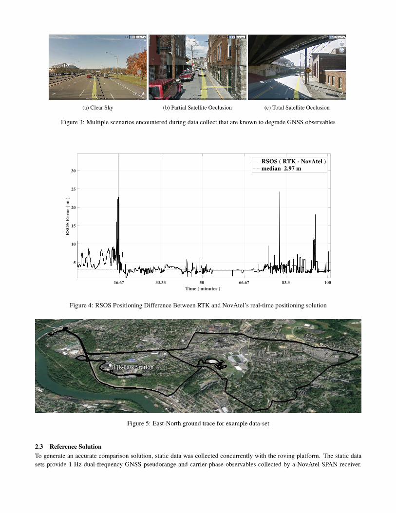
(a) Clear Sky (b) Partial Satellite Occlusion (c) Total Satellite Occlusion

Figure 3: Multiple scenarios encountered during data collect that are known to degrade GNSS observables

16.67 33.33 50 66.67 83.3 100

Time ( minutes )

5

10

15

20

25

30

RS

OS

Error (

m )

RSOS ( RTK - NovAtel )

median 2.97 m

Figure 4: RSOS Positioning Difference Between RTK and NovAtel’s real-time positioning solution

Figure 5: East-North ground trace for example data-set

2.3 Reference SolutionTo generate an accurate comparison solution, static data was collected concurrently with the roving platform. The static datasets provide 1 Hz dual-frequency GNSS pseudorange and carrier-phase observables collected by a NovAtel SPAN receiver.

This data is used to generate a Kalman filter/smoother Carrier-Phase Differential GPS (CP-DGPS) positioning solution withrespect to the local reference station. The CP-DGPS reference solution was calculated using RTKLIB (Takasu, 2009).

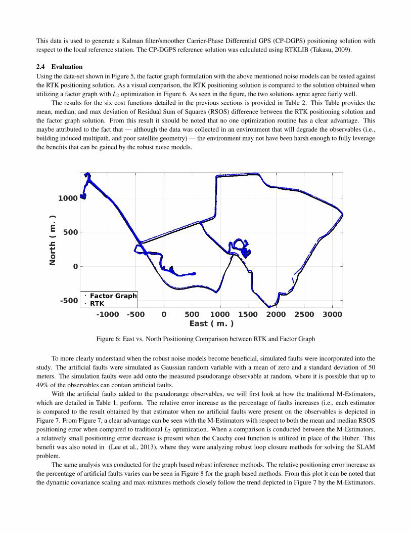
2.4 EvaluationUsing the data-set shown in Figure 5, the factor graph formulation with the above mentioned noise models can be tested againstthe RTK positioning solution. As a visual comparison, the RTK positioning solution is compared to the solution obtained whenutilizing a factor graph with L2 optimization in Figure 6. As seen in the figure, the two solutions agree agree fairly well.

The results for the six cost functions detailed in the previous sections is provided in Table 2. This Table provides themean, median, and max deviation of Residual Sum of Squares (RSOS) difference between the RTK positioning solution andthe factor graph solution. From this result it should be noted that no one optimization routine has a clear advantage. Thismaybe attributed to the fact that — although the data was collected in an environment that will degrade the observables (i.e.,building induced multipath, and poor satellite geometry) — the environment may not have been harsh enough to fully leveragethe benefits that can be gained by the robust noise models.

Figure 6: East vs. North Positioning Comparison between RTK and Factor Graph

To more clearly understand when the robust noise models become beneficial, simulated faults were incorporated into thestudy. The artificial faults were simulated as Gaussian random variable with a mean of zero and a standard deviation of 50meters. The simulation faults were add onto the measured pseudorange observable at random, where it is possible that up to49% of the observables can contain artificial faults.

With the artificial faults added to the pseudorange observables, we will first look at how the traditional M-Estimators,which are detailed in Table 1, perform. The relative error increase as the percentage of faults increases (i.e., each estimatoris compared to the result obtained by that estimator when no artificial faults were present on the observables is depicted inFigure 7. From Figure 7, a clear advantage can be seen with the M-Estimators with respect to both the mean and median RSOSpositioning error when compared to traditional L2 optimization. When a comparison is conducted between the M-Estimators,a relatively small positioning error decrease is present when the Cauchy cost function is utilized in place of the Huber. Thisbenefit was also noted in (Lee et al., 2013), where they were analyzing robust loop closure methods for solving the SLAMproblem.

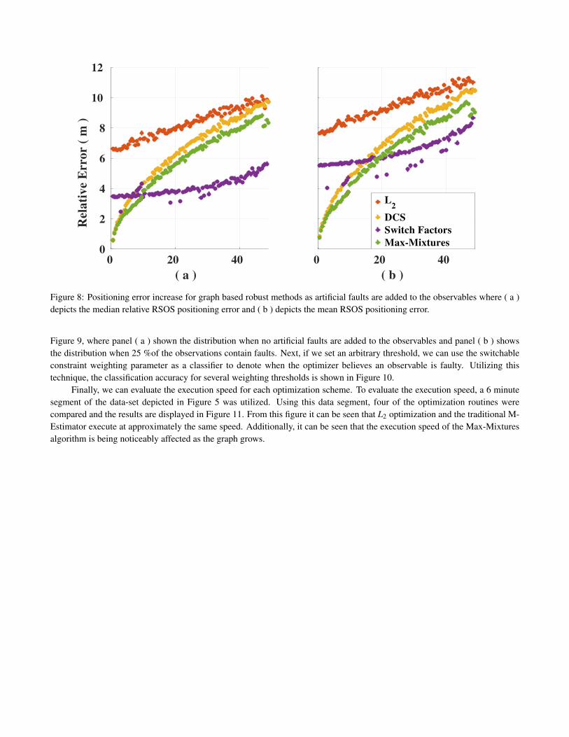
The same analysis was conducted for the graph based robust inference methods. The relative positioning error increase asthe percentage of artificial faults varies can be seen in Figure 8 for the graph based methods. From this plot it can be noted thatthe dynamic covariance scaling and max-mixtures methods closely follow the trend depicted in Figure 7 by the M-Estimators.

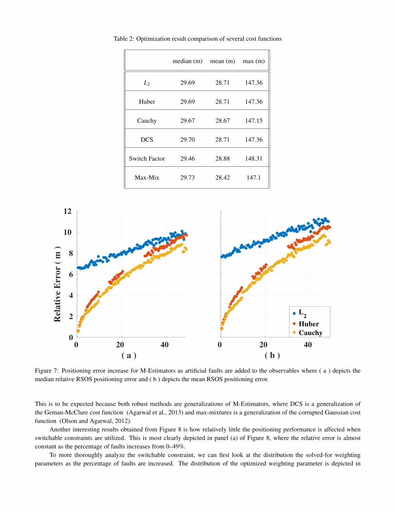
Table 2: Optimization result comparison of several cost functions

median (m) mean (m) max (m)

L2 29.69 28.71 147.36

Huber 29.69 28.71 147.36

Cauchy 29.67 28.67 147.15

DCS 29.70 28.71 147.36

Switch Factor 29.46 28.88 148.31

Max-Mix 29.73 28.42 147.1

0 20 40

( a )

0

2

4

6

8

10

12

Rela

tive E

rror (

m )

0 20 40

( b )

L2

Huber

Cauchy

Figure 7: Positioning error increase for M-Estimators as artificial faults are added to the observables where ( a ) depicts themedian relative RSOS positioning error and ( b ) depicts the mean RSOS positioning error.

This is to be expected because both robust methods are generalizations of M-Estimators, where DCS is a generalization ofthe Geman-McClure cost function (Agarwal et al., 2013) and max-mixtures is a generalization of the corrupted Gaussian costfunction (Olson and Agarwal, 2012).

Another interesting results obtained from Figure 8 is how relatively little the positioning performance is affected whenswitchable constraints are utilized. This is most clearly depicted in panel (a) of Figure 8, where the relative error is almostconstant as the percentage of faults increases from 0–49%.

To more thoroughly analyze the switchable constraint, we can first look at the distribution the solved-for weightingparameters as the percentage of faults are increased. The distribution of the optimized weighting parameter is depicted in

0 20 40

( a )

0

2

4

6

8

10

12

Rela

tive E

rror (

m )

0 20 40

( b )

L2

DCS

Switch Factors

Max-Mixtures

Figure 8: Positioning error increase for graph based robust methods as artificial faults are added to the observables where ( a )depicts the median relative RSOS positioning error and ( b ) depicts the mean RSOS positioning error.

Figure 9, where panel ( a ) shown the distribution when no artificial faults are added to the observables and panel ( b ) showsthe distribution when 25 %of the observations contain faults. Next, if we set an arbitrary threshold, we can use the switchableconstraint weighting parameter as a classifier to denote when the optimizer believes an observable is faulty. Utilizing thistechnique, the classification accuracy for several weighting thresholds is shown in Figure 10.

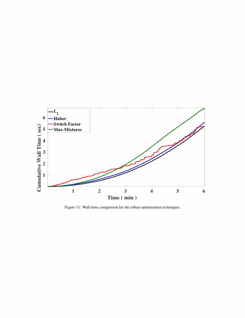
Finally, we can evaluate the execution speed for each optimization scheme. To evaluate the execution speed, a 6 minutesegment of the data-set depicted in Figure 5 was utilized. Using this data segment, four of the optimization routines werecompared and the results are displayed in Figure 11. From this figure it can be seen that L2 optimization and the traditional M-Estimator execute at approximately the same speed. Additionally, it can be seen that the execution speed of the Max-Mixturesalgorithm is being noticeably affected as the graph grows.

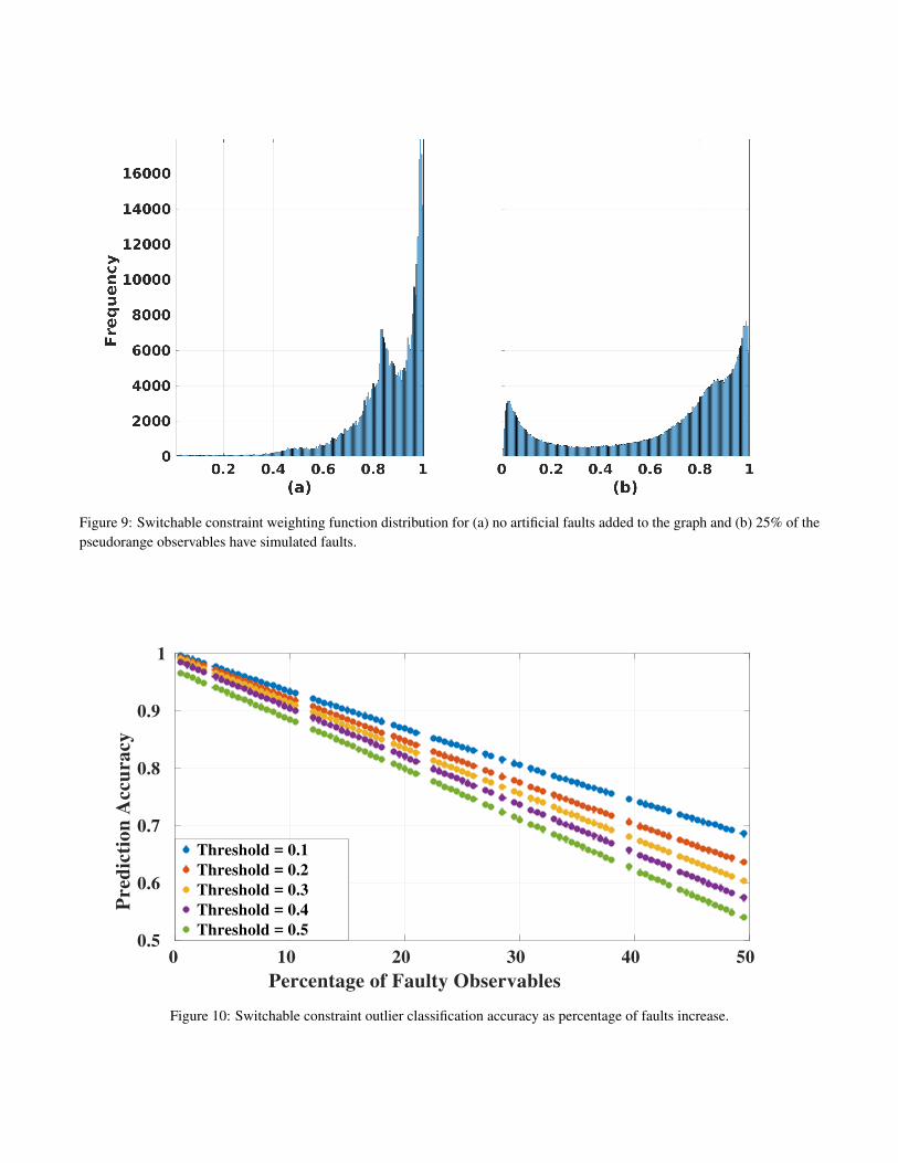
Figure 9: Switchable constraint weighting function distribution for (a) no artificial faults added to the graph and (b) 25% of thepseudorange observables have simulated faults.

0 10 20 30 40 50

Percentage of Faulty Observables

0.5

0.6

0.7

0.8

0.9

1

Pred

icti

on

Accu

racy

Threshold = 0.1

Threshold = 0.2

Threshold = 0.3

Threshold = 0.4

Threshold = 0.5

Figure 10: Switchable constraint outlier classification accuracy as percentage of faults increase.

1 2 3 4 5 6

Time ( min )

1

2

3

4

5

6

Cu

mu

lati

ve W

all

Tim

e (

sec)

L2

Huber

Switch Factor

Max-Mixtures

Figure 11: Wall-time comparison for the robust optimization techniques.

3 ConclusionFor autonomous navigation systems, there is a requirement that the system can robustly infer its desired states when confrontedwith adverse environments. To meet this requirement, we evaluated several robust optimization techniques from various fieldsfor the application of GNSS pseudorange data processing in an urban environment. From this analysis, it has been shown thattraditional M-Estimators can aid the optimization scheme when confronted with an adverse environment; however, it has alsobeen shown that including Switchable Constraints in the graph considerably outperforms the other methods implemented inthis study, specifically as the number of faulty observables increases.

Additionally, to allow the GNSS community to build upon the advances made within other research communities, the soft-ware developed and data sets used for this evaluation has been released publicly at https://github.com/wvu-navLab/RobustGNSS, which provides a GNSS front-end integrated with several robust noise models to the GTSAM library.

AcknowledgmentThe material in this report was approved for public release on the 26th of June 2017, case number 88ABW-2017-3109.

ReferencesP. Agarwal, G. Tipaldi, L. Spinello, C. Stachniss, and W. Burgard. Robust Map Optimization Using Dynamic Covariance

Scaling. In International Conference on Robotics and Automation, 2013.

H. Black and A. Eisner. Correcting Satellite Doppler Data for Tropospheric Effects. Journal of Geophysical Research, 89:2616, 1984.

F. Dellaert. Factor graphs and GTSAM: A hands-on introduction. Technical report, Georgia Institute of Technology, 2012.

P. Huber. Robust Estimation of a Location Parameter. The Annals of Mathematical Statistics, 35(1):73–101, 1964.

P. Huber. Robust Statistics. Wiley New York, 1981.

V. Indelmana, S. Williams, M. Kaess, and F. Dellaert. Information Fusion In Navigation Systems Via Factor Graph BasedIncremental Smoothing. In Robotics and Autonomous Systems, volume 61, 2013.

M. Kaess, V. Ila, R. Roberts, and F. Dellaert. The Bayes Tree: An Algorithmic Foundation for Probabilistic Robot Mapping.In Internation Workshop on the Algorithmic Foundations of Robotics, 2010.

M. Kaess, H. Johannsson, R. Roberts, V. Ila, J. Leonard, and F. Dellaert. iSAM2: Incremental Smoothing and Mapping Usingthe Bayes Tree. The International Journal of Robotics Research, 31(2), 2012.

R. E. Kalman. A New Approach to Linear Filtering and Prediction Problems. Transactions of the ASME–Journal of BasicEngineering, 82(Series D):35–45, 1960.

F. Kschischang and B. Frey. Factor Graphs and the Sum-Product Algorithm. In IEEE Transactions on Information Theory,volume 42, 2001.

G. H. Lee, F. Fraundorfer, and M. Pollefeys. Robust pose-graph loop-closures with expectation-maximization. In IntelligentRobots and Systems (IROS), 2013 IEEE/RSJ International Conference on, pages 556–563. IEEE, 2013.

M. Lourakis. A Brief Description of the Levenberg-Marquardt Algorithm Implemened by levmar. 2005.

P. Misra and P. Enge. Global Positioning System: Signals, Measurements and Performance Second Edition. Lincoln, MA:Ganga-Jamuna Press, 2006.

D. J. Olive. Applied Robust Statistics. Preprint M-02-006, 2008.

E. Olson and P. Agarwal. Inference on Networks of Mixtures for Robust Robot Mapping. 2012.

N. Sunderhauf and P. Protzel. Switchable Constraints for Robust Pose Graph SLAM. In Intelligent Robots and Systems, 2012.

N. Sunderhauf, M. Obst, G. Wanielik, and P. Protzel. Multipath mitigation in gnss-based localization using robust optimization.In Intelligent Vehicles Symposium (IV), 2012 IEEE, pages 784–789. IEEE, 2012.

N. Sunderhauf, M. Obst, S. Lange, G. Wanielik, and P. Protzel. Switchable constraints and incremental smoothing for onlinemitigation of non-line-of-sight and multipath effects. In Intelligent Vehicles Symposium (IV), 2013 IEEE, pages 262–268.IEEE, 2013.

T. Takasu. RTKLIB: Open Source Program Package for RTK-GPS. In FOSS4G 2009 Tokyo, Japan, November 2, 2009.

S. Thrun. Particle Filters in Robotics. In In Proceedings of Uncertainty in AI, 2002.

B. Tolman, R. B. Harris, T. Gaussiran, D. Munton, J. Little, R. Mach, S. Nelsen, and B. Renfro. The GPS Toolkit: OpenSource GPS Software. In Proceedings of the 16th International Technical Meeting of the Satellite Division of the Institute ofNavigation, Long Beach, California, 2004.

T. Whelan, M. Kaess, H. Johannsson, M. Fallon, J. Leonard, and J. McDonald. Real-Time Large-Scale Dense RGB-D SLAMWith Volumetric Fusion. The International Journal of Robotics Research, 34(4-5), 2015.