Robust Model Predictive Control:

A Survey

Alberto Bemporad and Manfred Morari

Automatic Control Laboratory, Swiss Federal Institute of Technology (ETH),Physikstrasse 3, CH-8092 Zurich, Switzerland,bemporad,morari@aut.ee.ethz.ch, http://control.ethz.ch/

Abstract. This paper gives an overview of robustness in Model Predictive Control(MPC). After reviewing the basic concepts of MPC, we survey the uncertaintydescriptions considered in the MPC literature, and the techniques proposed forrobust constraint handling, stability, and performance. The key concept of “closed-loop prediction” is discussed at length. The paper concludes with some commentson future research directions.

1 Introduction

Model Predictive Control (MPC), also referred to as Receding Horizon Con-trol and Moving Horizon Optimal Control, has been widely adopted in in-dustry as an effective means to deal with multivariable constrained controlproblems (Lee and Cooley 1997, Qin and Badgewell 1997). The ideas ofreceding horizon control and model predictive control can be traced back tothe 1960s (Garcia et al. 1989), but interest in this field started to surge onlyin the 1980s after publication of the first papers on IDCOM (Richalet etal. 1978) and Dynamic Matrix Control (DMC) (Cutler and Ramaker 1979,Cutler and Ramaker 1980), and the first comprehensive exposition of Gen-eralized Predictive Control (GPC) (Clarke et al. 1987a, Clarke et al. 1987b).Although at first sight the ideas underlying the DMC and GPC are simi-lar, DMC was conceived for multivariable constrained control, while GPCis primarily suited for single variable, and possibly adaptive control.

The conceptual structure of MPC is depicted in Fig. 1. The name MPCstems from the idea of employing an explicit model of the plant to be con-trolled which is used to predict the future output behavior. This predictioncapability allows solving optimal control problems on line, where trackingerror, namely the difference between the predicted output and the desiredreference, is minimized over a future horizon, possibly subject to constraintson the manipulated inputs and outputs. When the model is linear, then theoptimization problem is quadratic if the performance index is expressedthrough the `2-norm, or linear if expressed through the `1/`∞-norm. The

y(t)u(t)

PlantOptimizer

Reference

r(t)

OutputInput

Measurements

Fig. 1. Basic structure of Model Predictive Control

result of the optimization is applied according to a receding horizon philos-ophy: At time t only the first input of the optimal command sequence isactually applied to the plant. The remaining optimal inputs are discarded,and a new optimal control problem is solved at time t + 1. This idea isillustrated in Fig. 2. As new measurements are collected from the plant ateach time t, the receding horizon mechanism provides the controller withthe desired feedback characteristics.

The issues of feasibility of the on-line optimization, stability and perfor-mance are largely understood for systems described by linear models, as tes-tified by several books (Bitmead et al. 1990, Soeterboek 1992, Martın Sanchezand Rodellar 1996, Clarke 1994, Berber 1995, Camacho and Bordons 1995)and hundreds of papers (Kwon 1994)1. Much progress has been made onthese issues for nonlinear systems (Mayne 1997), but for practical appli-cations many questions remain, including the reliability and efficiency ofthe on-line computation scheme. Recently, application of MPC to hybridsystems integrating dynamic equations, switching, discrete variables, logicconditions, heuristic descriptions, and constraint prioritizations have beenaddressed by Bemporad and Morari (1999). They expanded the problem for-mulation to include integer variables, yielding a Mixed-Integer Quadratic orLinear Program for which efficient solution techniques are becoming avail-able.

A fundamental question about MPC is its robustness to model uncer-tainty and noise. When we say that a control system is robust we mean thatstability is maintained and that the performance specifications are met for aspecified range of model variations and a class of noise signals (uncertaintyrange). To be meaningful, any statement about “robustness” of a particu-lar control algorithm must make reference to a specific uncertainty range

1 Morari (1994) reports that a simple database search for “predictive control”generated 128 references for the years 1991-1993. A similar search for the years1991-1998 generated 2802 references.

Fig. 2. Receding horizon strategy: only the first one of the computed moves u(t)is implemented

as well as specific stability and performance criteria. Although a rich the-ory has been developed for the robust control of linear systems, very little isknown about the robust control of linear systems with constraints. Recently,this type of problem has been addressed in the context of MPC. This paperwill give an overview of these attempts to endow MPC with some robustnessguarantees. The discussion is limited to linear time invariant (LTI) systemswith constraints. While the use of MPC has also been proposed for LTIsystems without constraints, MPC does not have any practical advantagein this case. Many other methods are available which are at least equallysuitable.

2 MPC Formulation

In the research literature MPC is formulated almost always in the statespace. Let the model Σ of the plant to be controlled be described by thelinear discrete-time difference equations

Σ :

x(t+ 1) = Ax(t) +Bu(t), x(0) = x0,

y(t) = Cx(t)(1)

where x(t) ∈ Rn, u(t) ∈ Rm, y(t) ∈ Rp denote the state, control input, andoutput respectively. Let x(t + k, x(t), Σ) or, in short, x(t + k|t) denote theprediction obtained by iterating model (1) k times from the current statex(t).

A receding horizon implementation is typically based on the solution ofthe following open-loop optimization problem:

minU , u(t+ k|t)t+Nm−1

k=t

J(U, x(t), Np, Nm) = xT (Np)P0x(Np)

+

Np−1∑k=0

x′(t+ k|t)Qx(t+ k|t) +

Nm−1∑k=0

u′(t+ k|t)Ru(t+ k|t)

(2a)

subject toF1u(t+ k|t) ≤ G1

E2x(t+ k|t)+ F2u(t+ k|t) ≤ G2(2b)

and“stability constraints” (2c)

where, as shown in Fig. 2, Np denotes the length of the prediction hori-zon or output horizon, and Nm denotes the length of the control horizonor input horizon (Nm ≤ Np). When Np = ∞, we refer to this as the in-finite horizon problem, and similarly, when Np is finite, as a finite horizonproblem. For the problem to be meaningful we assume that the polyhedron(x, u) : F1u ≤ G1, E2x + F2u ≤ G2 contains the origin (x = 0, u = 0).The constraints (2c) are inserted in the optimization problem in order toguarantee closed-loop stability, and will be discussed in the sequel.

The basic MPC law is described by the following algorithm:

Algorithm 1:

1. Get the new state x(t)2. Solve the optimization problem (2)3. Apply only u(t) = u(t+ 0|t)4. t← t+ 1. Go to 1.

2.1 Some Important Issues

Feasibility Feasibility of the optimization problem (2) at each time t mustbe ensured. Typically one assumes feasibility at time t = 0 and chooses thecost function (2a) and the stability constraints (2c) such that feasibility ispreserved at the following time steps. This can be done, for instance, byensuring that the shifted optimal sequence u(t+ 1|t), . . . , u(t+Np|t), 0 isfeasible at time t + 1. Also, typically the constraints in (2b) which involve

state components are treated as soft constraints, for instance by adding theslack variable ε

E2x+ F2u ≤ G2 + ε

[1...1

], (3)

while pure input constraints F1u ≤ G1 are maintained as hard. Relaxing thestate constraints removes the feasibility problem at least for stable systems.Keeping the state constraints tight does not make sense from a practicalpoint of view because of the presence of noise, disturbances, and numericalerrors. As the inputs are generated by the optimization procedure, the inputconstraints can always be regarded as hard.

Stability In the MPC formulation (2) we have not specified the stabilityconstraints (2c). Below we review some of the popular techniques used inthe literature to “enforce” stability. They can be divided into two mainclasses. The first uses the value V (t) = J(U∗, x(t), Np, Nm) attained for the

minimizer U∗ , u∗(t + 1|t), . . . , u∗(t + Nm|t) of (2) at each time t asa Lyapunov function. The second explicitly requires that the state x(t) isshrinking in some norm.

• End (Terminal) Constraint (Kwon and Pearson 1977, Kwon and Pearson1978). The stability constraint (2c) is

x(t+Np|t) = 0 (4)

This renders the sequence U1 , u∗(t + 1|t), . . . , u∗(t + Nm|t), 0 fea-sible at time t+ 1, and therefore V (t+ 1) ≤ J(U1, x(t+ 1), Np, Nm) ≤J(U∗, x(t), Np, Nm) = V (t) is a Lyapunov function of the system (Keerthiand Gilbert 1988, Bemporad et al. 1994).The main drawback of using terminal constraints is that the controleffort required to steer the state to the origin can be large, especiallyfor short Np, and therefore feasibility is more critical because of (2b).The domain of attraction of the closed-loop (MPC+plant) is limited tothe set of initial states x0 that can be steered to 0 in Np steps whilesatisfying (2b), which can be considerably smaller then the set of initialstates steerable to the origin in an arbitrary number of steps. Also, per-formance can be negatively affected because of the artificial terminalconstraint. A variation of the terminal constraint idea has been pro-posed where only the unstable modes are forced to zero at the end ofthe horizon (Rawlings and Muske 1993). This mitigates some of thementioned problems.• Infinite Output Prediction Horizon (Keerthi and Gilbert 1988, Rawlings

and Muske 1993, Zheng and Morari 1995). For asymptotically stablesystems, no stability constraint is required if Np = +∞. The proof isagain based on a similar Lyapunov argument.

• Terminal Weighting Matrix (Kwon et al. 1983, Kwon and Byun 1989).By choosing the terminal weighting matrix P0 in (2a) as the solution ofa Riccati inequality, stability can be guaranteed without the addition ofstability constraints.• Invariant terminal set (Scokaert and Rawlings 1996). The idea is to

relax the terminal constraint (4) into the set-membership constraint

x(t+Np|t) ∈ Ω (5)

and set u(t + k|t) = FLQx(t + k|t), ∀k ≥ Nm, where FLQ is the LQfeedback gain. The set Ω is invariant under LQ regulation and such thatthe constraints are fulfilled inside Ω. Again, stability can be proved viaLyapunov arguments.• Contraction Constraint (Polak and Yang 1993a, Zheng 1995). Rather

then relying on the optimal cost V (t) as a Lyapunov function, the ideais to require explicitly that the state x(t) is decreasing in some norm

‖x(t+ 1|t)‖ ≤ α‖x(t)‖, α < 1 (6)

Following this idea, Bemporad (1998a) proposed a technique where sta-bility is guaranteed by synthesizing a quadratic Lyapunov function forthe system, and by requiring that the terminal state lies within a levelset of the Lyapunov function, similar to (5).

Computation The complexity of the solver for the optimization prob-lem (2) depends on the choice of the performance index and the stabil-ity constraint (2c). When Np = +∞, or the stability constraint has theform (4), or the form (5) and Ω is a polytope, the optimization problem (2)is a Quadratic Program (QP). Alternatively, one obtains a Linear Program(LP) by formulating the performance index (2a) in ‖ · ‖1 or ‖ · ‖∞ (Campoand Morari 1989). The constraint (6) is convex, and is quadratic or linear de-pending if ‖·‖2 or ‖·‖1/‖·‖∞ is chosen. When ‖·‖2 is used, second-order coneprogramming algorithms (Lobo et al. 1997) can be adopted conveniently.

3 Robust MPC — Problem Definition

The basic MPC algorithm described in the previous section assumes thatthe plant Σ0 to be controlled and the model Σ used for prediction andoptimization are the same, and no unmeasured disturbance is acting on thesystem. In order to talk about robustness issues, we have to relax thesehypotheses and assume that (i) the true plant Σ0 ∈ S, where S is a givenfamily of LTI systems, and/or (ii) an unmeasured noise w(k) enters thesystem, namely

Σ :

x(t+ 1) = Ax(t) +Bu(t) +Hw(t), x(0) = x0,

y(t) = Cx(t) +Kw(t)(7)

where w(t) ∈ W and W is a given set (usually a polytope).We will refer to robust stability, robust constraint fulfillment, and robust

performance of the MPC law if the respective property is guaranteed for allpossible Σ0 ∈ S, w(t) ∈ W .

As part of the modelling effort it is necessary to arrive at an appropriatedescription of the uncertainty, i.e. the sets S andW . This is difficult becausethere is very little experience and no systematic procedures are available.On one hand, the uncertainty description should be “tight”, i.e. it shouldnot include “extra” plants which do not exist in the real situation. On theother hand, there is a trade-off between realism and the resulting compu-tational complexity of the analysis and controller synthesis. In other words,the uncertainty description should lead to a simple (non-conservative) anal-ysis procedure to determine if a particular system with controller is stableand meets the performance requirements in the presence of the specifieduncertainty. Alternatively, a computationally tractable synthesis procedureshould exist to design a controller which is robustly stable and satisfies therobust performance specifications.

At present all the proposed uncertainty descriptions and associated anal-ysis/synthesis procedures do little more than provide different handle to theengineer to detect and avoid sensitivity problems. They do not address thetrade-off alluded to above, in a systematic manner.

For example, for simplicity some procedures consider only the uncer-tainty introduced by the set of unmeasured bounded inputs. There is theimplicit assumptions that the other model uncertainty is in some way cov-ered in this manner. There has been no rigorous analysis, however, to de-termine the exact relationship between the input setW and the covered setS — if such a relationship does indeed exist.

In the remaining part of the paper we will describe the different uncer-tainty descriptions which have been used in robust MPC, comment on therobustness analysis of standard (no uncertainty description) MPC, and givean overview of the problems associated with the synthesis of robust MPCcontrol laws.

4 Uncertainty Descriptions

Different uncertainty sets S, W have been proposed in the literature inthe context of MPC, and are mostly based on time-domain representations.Frequency-domain descriptions of uncertainty are not suitable for the formu-lation of robust MPC because MPC is primarily a time-domain technique.

4.1 Impulse/Step-Response

Uncertainties on the impulse-response or step-response coefficients providea practical description in many applications, as they can be easily deter-

Fig. 3. Step-response interval ranges (right) arising from an impulse-responsedescription (left)

mined from experimental tests, and allow a reasonably simple way to com-pute robust predictions. Uncertainty is described as range intervals overthe coefficients of the impulse- and/or step-response. In the simplest SISO(single-input single-output) case, this corresponds to set

Σ : y(t) =

N∑k=0

h(t)u(t− k) (8)

and

S = Σ : h−t ≤ h(t) ≤ h+t , t = 0, . . . , N (9)

where [h−t , h+t ] are given intervals. For N <∞, S is a set of FIR models.

A similar type of description can be used for step-response models

y(t) =

N∑k=0

s(t)[u(t− k)− u(t− k − 1)], s(t) ∈ [s−t , s+t ] (10)

Impulse- and step-response descriptions are only equivalent when thereis no uncertainty. If there is uncertainty they behave rather differently(Bemporad and Mosca 1998). In order to arrive at a tight uncertainty de-scription both may have to be used simultaneously and further constraintsmay have to be imposed on the coefficient variations as we will explain.

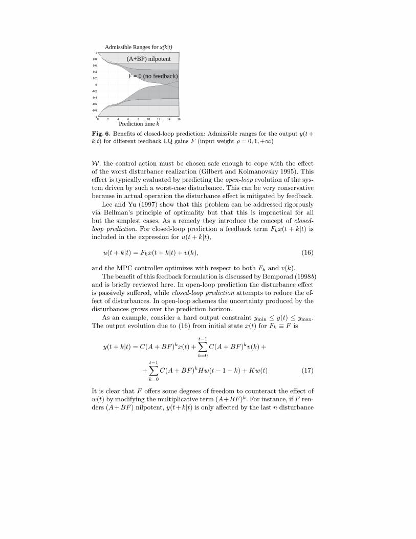
Consider Fig. 3, which depicts perturbations expressed only in termsof the impulse response. The resulting step-response uncertainty is verylarge as t → ∞. This may not be a good description of the real situation.Conversely, as depicted in Fig. 4, uncertainty expressed only in terms ofthe step response could lead to nonzero impulse-response samples at largevalues of t, for instance because the DC-gain from u to y is uncertain. Henceany a priori information about asymptotic stability properties would not beexploited.

Also, the proposed bounds would allow the step response to be highlyoscillatory, though the process may be known to be overdamped. Similarcomments apply to the impulse response. Thus this description may in-troduce high frequency model uncertainty artificially and may lead to a

Fig. 4. Impulse-response interval ranges (left) arising from a step-response de-scription (right)

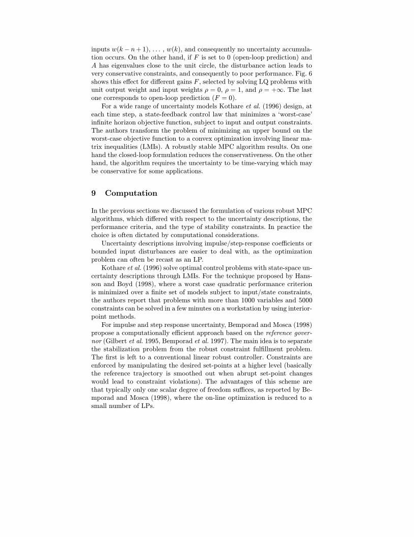
Fig. 5. Structured feedback uncertainty

conservative design. This deficiency can be alleviated by imposing a cor-relation between neighboring uncertain coefficients as proposed by Zheng(1995).

Another subtle point is that the uncertain FIR model (8) is usuallyunsuitable if the coefficients must be assumed to be time varying in theanalysis or synthesis. In this case, the model would predict output variationseven when the input is constant, which is usually undesirable. Writing themodel in the form

Σ : y(t) = y(t− 1) +

N∑k=0

h(t)[u(t− k)− u(t− k − 1)] (11)

removes this problem.In conclusion, simply allowing the step- or impulse-response coefficients

to vary within intervals is rarely a useful description of model uncertaintyunless additional precautions are taken. Nevertheless, compared to otherdescriptions, it leads to computationally simpler algorithms when adoptedin robust MPC design, as will be discussed in Sect. 9

4.2 Structured Feedback Uncertainty

A common paradigm for robust control consists of a linear time-invariantsystem with uncertainties in the feedback loop, as depicted in Fig. 5 (Kothareet al. 1996). The operator ∆ is block-diagonal, ∆ = diag∆1, . . . , ∆r,where each block ∆i represents either a memoryless time-varying matrix

with ‖∆i(t)‖2 = σ(∆i(t)) ≤ 1, ∀i = 1, . . . , r, t ≥ 0; or a convolution op-erator (e.g. a stable LTI system) with the operator norm induced by thetruncated `2-norm less than 1, namely

∑tj=0 p

′(j)p(j) ≤∑tj=0 q

′(j)q(j),∀t ≥ 0. When ∆i are stable LTI systems, this corresponds to the frequencydomain specification on the z-transform ∆i(z) ‖∆(z)‖H∞ < 1.

4.3 Multi-Plant

We refer to a multi-plant description when model uncertainty is parameter-ized by a finite list of possible plants (Badgwell 1997)

Σ ∈ Σ1, . . . , Σn (12)

When we allow the real system to vary within the convex hull defined bythe list of possible plants we obtain the so called polytopic uncertainty.

4.4 Polytopic Uncertainty

The set of models S is described as

x(t+ 1) = A(t)x(t) +B(t)u(t)y(t) = Cx(t)

[A(t) B(t)] ∈ Ω

and Ω = Co[A1 B1], . . . , [AM BM ], the convex hull of the “extreme”models [Ai Bi] is a polytope. As remarked by Kothare et al. (1996), poly-topic uncertainty is a conservative approach to model a nonlinear systemx(t+ 1) = f(x(k), u(k), k) when the Jacobian [∂f

∂x∂f∂u

] is known to lie in thepolytope Ω.

4.5 Bounded Input Disturbances

The uncertainty is limited to the unknown disturbance w ∈ W in (7), theplant Σ0 is assumed to be known (S = Σ0). Also, one assumes thatbounds on the disturbance are known, i.e. W is a given set. Although theassumption of knowing model Σ0 might seem restrictive, the description ofuncertainty by additive terms w(t) that are known to be bounded in somenorm is a reasonable choice, as shown in the recent literature on robustcontrol and identification (Milanese and Vicino 1993, Makila et al. 1995).

5 Robustness Analysis

We distinguish robustness analysis, i.e. analysis of the robustness proper-ties of standard MPC designed for a nominal model without taking into

account uncertainty, and synthesis of MPC algorithms which are robust byconstruction.

The robustness analysis of MPC control loops is more difficult than thesynthesis, where the controller is designed in such a way that it is robustlystabilizing. This is not unlike the situation in the nominal case where thestability analysis of a closed loop MIMO system with multiple constraintsis essentially impossible. On the other hand, the MPC technology leadsnaturally to a controller such that the closed loop system is guaranteed tobe stable. There is a need for analysis tools, however, because standard MPCalgorithms typically require less on-line computations, which is desirable forimplementation.

Indeed, there are very few analysis methods discussed in the literature.By using a contraction mapping theorem, Zafiriou (1990) derives a set ofsufficient conditions for nominal and robust stability of MPC. Because theconditions are difficult to check he also states some necessary conditions forthese sufficient conditions.

Genceli and Nikolaou (1993) give sufficient conditions for robust closed-loop stability and investigate robust performance of dynamic matrix control(DMC) systems with hard input/soft output constraints. The authors con-sider an `1-norm performance index, a terminal state condition as a stabilityconstraint, an impulse-response model with bounds on the variations of thecoefficients. They derive a robustness test in terms of simple inequalities tobe satisfied. This simplicity is largely lost in the extension to the MIMOcase.

Primbs and Nevistıc (1998) provide an off-line robustness analysis testof constrained finite receding horizon control which requires the solution ofa set of linear matrix inequalities (LMIs). The test is based on the so calledS-procedure and provides a (conservative) sufficient condition for V (t) tobe decreasing for all Σ ∈ S, ∀w(t) ∈ W . Both polytopic and structureduncertainty descriptions are considered. The authors also extend the ideato develop a robust synthesis method. It requires the solution of bilinearmatrix inequalities (BMIs) and is computationally demanding.

More recently, Primbs (1999) presented a new formulation of the analysistechnique which is less conservative. The idea is to express the (optimal)input u(t) obtained by the MPC law through the Lagrangian multipliersλ associated with the optimization problem (2a), and then to write theS-procedure in the [x, u, λ]-space.

6 Robust MPC Synthesis

In light of the discussion in Section 2.1, one has the following alternativeswhen synthesizing robust MPC laws:

1. Optimize performance of the nominal model or robust performance ?2. Enforce state constraints on the nominal model or robustly ?

3. Adopt an open-loop or a closed-loop prediction scheme ?4. How to guarantee robust stability ?

In the remaining part of the section we will discuss these questions.

6.1 Nominal vs. Robust Performance

The performance index (2a) depends on one particular model Σ and dis-turbance realization w(t). In an uncertainty framework, two strategies arepossible: (i) define a nominal model Σ and nominal disturbance w(t) = 0,and optimize nominal performance; or (ii) solve the min-max problem tooptimize robust performance

minU

maxΣ ∈ S

w(k + t)Np−1

k=0⊆ W

J(U, x(t), Σ, w(·)) (13)

Min-max robust MPC was first proposed by Campo and Morari (1987),and further developed by Allwright and Papavasiliou (1992) and Zhengand Morari (1993) for SISO FIR plants. Kothare et al. (1996) optimizerobust performance for polytopic/multi-model and structured feedback un-certainty, Scokaert and Mayne (1998) for input disturbances only, and Leeand Yu (1997) for linear time-varying and time-invariant state-space modelsdepending on a vector of parameters θ ∈ Θ, where Θ is either an ellipsoidor a polyhedron. However it has two possible drawbacks. The first one iscomputational: Solving the problem (13) is computationally much more de-manding than solving (2a) for a nominal model Σ, w(t) = 0. However, underslightly restrict assumptions on the uncertainty, quite efficient algorithmsare possible (Zheng 1995). The second one is that the control action maybe excessively conservative.

6.2 Input and State Constraints

In the presence of uncertainty, the constraints on the states variables (2b)can be enforced for all plant Σ ∈ S (robust constraint fulfillment) or for anominal system Σ only. One also has to distinguish between hard and softstate constraints, although the latter are preferable for the reasons discussedin Section 2.1. As command inputs are directly generated by the optimizer,input constraints do not present any additional difficulty relative to thenominal MPC case.

For uncertainty described in terms of w(t) ∈ W only, when the setW is apolyhedron, state constraints can be tackled through the theory of maximaloutput admissible sets MOAS developed by (Gilbert and Tan 1991), Gilbertet al. (1995). The theory provides tools to enforce hard constraints on statesdespite the presence of input disturbances, by computing the minimum out-put prediction horizon Np which guarantees robust constraint fulfillment.

Mayne and Schroeder (1997) and (Scokaert and Mayne 1998) use toolsfrom MOAS theory to synthesize robust minimum-time control on line. Thetechnique is based on the computation of the level sets of the value function,and deals with hard input/state constraints.

Bemporad and Garulli (1997) also consider the effect of the worst in-put disturbance over the prediction horizon, and enforce constraint ful-fillment for all possible disturbance realizations (output prediction hori-zons are again computed through algorithms inspired by MOAS theory).In addition, the authors consider the case when full state information isnot available. They use the so-called set-membership (SM) state estimation(Schweppe 1968, Bertsekas and Rhodes 1971), through recursive algorithmsbased on parallelotopic approximation of the state uncertainty set (Vicinoand Zappa 1996, Chisci et al. 1996).

When impulse-response descriptions are adopted, output constraints canbe easily related to the uncertainty intervals of the impulse-response coef-ficients. For embedding input and state constraint into LMIs, the reader isreferred to Kothare et al. (1996).

Robust fulfillment of state constraints can result in a very conservativebehavior. Such an undesirable effect can be mitigated by using closed-loopprediction (see Sect. 8). Alternatively, when violations of the constraints areallowed, it can be more convenient to impose constraint satisfaction on thenominal plant Σ only.

Although unconstrained MPC for uncertain systems has been investi-gated, we do not review this literature here, because many superior linearrobust control techniques are available.

7 Robust Stability

The minimum closed-loop requirement is robust stability, i.e., stability inthe presence of uncertainty. In MPC the various design procedures achieverobust stability in two different ways: indirectly by specifying the perfor-mance objective and uncertainty description in such a way that the optimalcontrol computations lead to robust stability; or directly by enforcing a typeof robust contraction constraint which guarantees that the state will shrinkfor all plants in the uncertainty set.

7.1 Min-max performance optimization

While the generalization (13) of nominal MPC to the robust case appearsnatural, it is not without pitfalls. The min-max formulation as proposedby Campo and Morari (1987) alone does not guarantee robust stability aswas demonstrated by Zheng (1995) through a counterexample. To ensurerobust stability the uncertainty must be assumed to be time varying. Thisadded conservativeness may be prohibitive for demanding applications.

7.2 Robust contraction constraint

For stable plants, Zheng (1995) introduces the stability constraint

‖x(t+ 1|t)‖P ≤ λ‖x(t)‖P , λ < 1. (14)

which forces the state to contract. When P 0 is chosen as the solution ofthe Lyapunov equation A′PA − P = −Q, Q 0, then this constraint canalways be met for some u (u(t + k) = 0 satisfies this constraint and anyconstraint on u). Zheng (1995) achieves robust stability by requiring thestate to contract for all plants in S. For the uncertain case constraint (14)is generalized by maximizing ‖x(t+ 1|t)‖P over Σ ∈ S.

For the multi-plant description, Badgwell (1997) proposes a robust MPCalgorithm for stable, constrained, linear plants that is a direct generalizationof the nominally stabilizing regulator presented by Rawlings and Muske(1993). By using Lyapunov arguments, robust stability can be proved whenthe following stability constraint is imposed for each plant in the set.

J(U, x(t), Σi) ≤ J(U∗1, x(t), Σi) (15)

This can be seen as a special case of the contraction constraint, whereJ(U, x(t), Σi) is the cost associated with the prediction model Σi for afixed pair (Np, Nm), and U1 , u∗(t|t− 1), . . . , u∗(t− 1 +Nm|t− 1), 0 isthe shifted optimal sequence computed at time t−1. Note that the stabilityconstraints (15) are quadratic.

7.3 Robustly Invariant Terminal Sets

Invariant ellipsoidal terminal sets have been proposed recently in the nom-inal context as relaxations of the terminal equality constraint mentioned inSection 2.1 (see for instance (Bemporad 1998a) and references therein). Suchtechniques can be extended to robust MPC formulations, for instance byusing the LMI techniques developed by Kothare et al. (1996). Invariant ter-minal ellipsoid inevitably lead to Quadratically Constrained Quadratic Pro-grams (QCQP), which can be solved through interior-point methods (Loboet al. 1997). Alternatively, one can determine polyhedral robustly terminalinvariant sets (Blanchini 1999), which would lead to linear constraints, andtherefore quadratic programming (QP), which is computationally cheaperthan QCQP, at least for small/medium size problems.

8 Closed-Loop Prediction

Let us consider the design of a predictive controller which guarantees thathard state constraints are met in the presence of input disturbances w(t). Inorder to achieve this task for every possible disturbance realization w(t) ∈

0 2 4 6 8 10 12 14 16-1

-0.8

-0.6

-0.4

-0.2

0

0.2

0.4

0.6

0.8

1

Admissible Ranges forx(k|t)Admissible Ranges forx(k|t)

Prediction timekPrediction timek

F = 0 (no feedback)

(A+BF) nilpotent

Fig. 6. Benefits of closed-loop prediction: Admissible ranges for the output y(t+k|t) for different feedback LQ gains F (input weight ρ = 0, 1,+∞)

W , the control action must be chosen safe enough to cope with the effectof the worst disturbance realization (Gilbert and Kolmanovsky 1995). Thiseffect is typically evaluated by predicting the open-loop evolution of the sys-tem driven by such a worst-case disturbance. This can be very conservativebecause in actual operation the disturbance effect is mitigated by feedback.

Lee and Yu (1997) show that this problem can be addressed rigorouslyvia Bellman’s principle of optimality but that this is impractical for allbut the simplest cases. As a remedy they introduce the concept of closed-loop prediction. For closed-loop prediction a feedback term Fkx(t + k|t) isincluded in the expression for u(t+ k|t),

u(t+ k|t) = Fkx(t+ k|t) + v(k), (16)

and the MPC controller optimizes with respect to both Fk and v(k).

The benefit of this feedback formulation is discussed by Bemporad (1998b)and is briefly reviewed here. In open-loop prediction the disturbance effectis passively suffered, while closed-loop prediction attempts to reduce the ef-fect of disturbances. In open-loop schemes the uncertainty produced by thedisturbances grows over the prediction horizon.

As an example, consider a hard output constraint ymin ≤ y(t) ≤ ymax.The output evolution due to (16) from initial state x(t) for Fk ≡ F is

y(t+ k|t) = C(A +BF )kx(t) +t−1∑k=0

C(A+BF )kv(k) +

+

t−1∑k=0

C(A+BF )kHw(t− 1− k) +Kw(t) (17)

It is clear that F offers some degrees of freedom to counteract the effect ofw(t) by modifying the multiplicative term (A+BF )k. For instance, if F ren-ders (A+BF ) nilpotent, y(t+k|t) is only affected by the last n disturbance

inputs w(k− n+ 1), . . . , w(k), and consequently no uncertainty accumula-tion occurs. On the other hand, if F is set to 0 (open-loop prediction) andA has eigenvalues close to the unit circle, the disturbance action leads tovery conservative constraints, and consequently to poor performance. Fig. 6shows this effect for different gains F , selected by solving LQ problems withunit output weight and input weights ρ = 0, ρ = 1, and ρ = +∞. The lastone corresponds to open-loop prediction (F = 0).

For a wide range of uncertainty models Kothare et al. (1996) design, ateach time step, a state-feedback control law that minimizes a ‘worst-case’infinite horizon objective function, subject to input and output constraints.The authors transform the problem of minimizing an upper bound on theworst-case objective function to a convex optimization involving linear ma-trix inequalities (LMIs). A robustly stable MPC algorithm results. On onehand the closed-loop formulation reduces the conservativeness. On the otherhand, the algorithm requires the uncertainty to be time-varying which maybe conservative for some applications.

9 Computation

In the previous sections we discussed the formulation of various robust MPCalgorithms, which differed with respect to the uncertainty descriptions, theperformance criteria, and the type of stability constraints. In practice thechoice is often dictated by computational considerations.

Uncertainty descriptions involving impulse/step-response coefficients orbounded input disturbances are easier to deal with, as the optimizationproblem can often be recast as an LP.

Kothare et al. (1996) solve optimal control problems with state-space un-certainty descriptions through LMIs. For the technique proposed by Hans-son and Boyd (1998), where a worst case quadratic performance criterionis minimized over a finite set of models subject to input/state constraints,the authors report that problems with more than 1000 variables and 5000constraints can be solved in a few minutes on a workstation by using interior-point methods.

For impulse and step response uncertainty, Bemporad and Mosca (1998)propose a computationally efficient approach based on the reference gover-nor (Gilbert et al. 1995, Bemporad et al. 1997). The main idea is to separatethe stabilization problem from the robust constraint fulfillment problem.The first is left to a conventional linear robust controller. Constraints areenforced by manipulating the desired set-points at a higher level (basicallythe reference trajectory is smoothed out when abrupt set-point changeswould lead to constraint violations). The advantages of this scheme arethat typically only one scalar degree of freedom suffices, as reported by Be-mporad and Mosca (1998), where the on-line optimization is reduced to asmall number of LPs.

10 Conclusions and Research Directions

While this review is not complete it reflects the state of the art. It is appar-ent that none of the methods presented is suitable for use in industry exceptmaybe in very special situations. The techniques are hardly an alternativeto ad hoc MPC tuning based on exhaustive simulations for ranges of oper-ating conditions. Choosing the right robust MPC technique for a particularapplication is an art and much experience is necessary to make it work —even on a simulation case study. Much research remains to be done, but theproblems are difficult. Some topics for investigation are suggested next.

Contraction constraints have been shown to be successful tools to getstability guarantees, but typically performance suffers. By forcing the stateto decrease in a somewhat arbitrary manner, the evolution is driven awayfrom optimality as measured by the performance index. The contraction con-straints which are in effect Lyapunov functions are only sufficient for stabil-ity. In principle, less restrictive criteria could be found. Integral QuadraticConstraints (Megretski and Rantzer 1997) could be embedded in robustMPC in order to deviate as little as possible from optimal performance butstill guarantee robust stability.

Robustly invariant terminal sets can be adopted as an alternative tocontraction constraints. As mentioned in Sect. 7, ellipsoids and polyhedracan be determined off-line, by utilizing tools from robustly invariant settheories (Blanchini 1999).

The benefits of closed-loop prediction were addressed in Sect. 8. Howeververy little research has been done toward the development of computation-ally efficient MPC algorithms.

Finally, the algorithms should be linked to appropriate identificationprocedures for obtaining the models and the associated uncertainty descrip-tions.

Acknowledgments

The authors thank Dr. James A. Primbs and Prof. Alexandre Megretski foruseful discussions. Alberto Bemporad was supported by the Swiss NationalScience Foundation.

References

Allwright, J. C. (1994). On min-max model-based predictive control. In: Advancesin Model-Based Predictive Control. pp. 415–426. Oxford Press Inc.,N. Y.. NewYork.

Allwright, J.C. and G.C. Papavasiliou (1992). On linear programming and robustmodel-predictive control using impulse-responses. Systems & Control Letters18, 159–164.

Badgwell, T. A. (1997). Robust model predictive control of stable linear systems.Int. J. Control 68(4), 797–818.

Bemporad, A. (1998a). A predictive controller with artificial Lyapunov functionfor linear systems with input/state constraints. Automatica 34(10), 1255–1260.

Bemporad, A. (1998b). Reducing conservativeness in predictive control of con-strained systems with disturbances. In: Proc. 37th IEEE Conf. on Decisionand Control. Tampa, FL. pp. 1384–1391.

Bemporad, A., A. Casavola and E. Mosca (1997). Nonlinear control of constrainedlinear systems via predictive reference management. IEEE Trans. AutomaticControl AC-42(3), 340–349.

Bemporad, A. and A. Garulli (1997). Predictive control via set-membership stateestimation for constrained linear systems with disturbances. In: Proc. Euro-pean Control Conf.. Bruxelles, Belgium.

Bemporad, A. and E. Mosca (1998). Fulfilling hard constraints in uncertain linearsystems by reference managing. Automatica 34(4), 451–461.

Bemporad, A. and M. Morari (1999). Control of systems integrat-ing logic, dynamics, and constraints. Automatica 35(3), 407–427.ftp://control.ethz.ch/pub/reports/postscript/AUT98-04.ps.

Bemporad, A., L. Chisci and E. Mosca (1994). On the stabilizing property of thezero terminal state receding horizon regulation. Automatica 30(12), 2013–2015.

Benvenuti, L. and L. Farina (1998). Constrained control for uncertain discrete-time linear systems. Int. J. Robust Nonlinear Control 8, 555–565.

Berber, R., Ed.) (1995). Methods of Model Based Process Control. Vol. 293of NATO ASI Series E: Applied Sciences. Kluwer Academic Publications.Dortrecht, Netherlands.

Bertsekas, D.P. and I.B. Rhodes (1971). Recursive state estimation for a set-membership description of uncertainty. IEEE Trans. Automatic Control16, 117–128.

Bitmead, R. R., M. Gevers and V. Wertz (1990). Adaptive Optimal Control. TheThinking Man’s GPC. International Series in Systems and Control Engineer-ing. Prentice Hall.

Blanchini, F. (1990). Control synthesis for discrete time systems with control andstate bounds in the presence of disturbances. J. of Optimization Theory andApplications 65(1), 29–40.

Blanchini, F. (1999). Set invariance in control — a survey. Automatica. In press.Camacho, E.F. and C. Bordons (1995). Model Predictive Control in the Process

Industry. Advances in Industrial Control. Springer Verlag.Campo, P.J. and M. Morari (1987). Robust model predictive control. In: Proc.

American Contr. Conf.. Vol. 2. pp. 1021–1026.Campo, P.J. and M. Morari (1989). Model predictive optimal averaging level con-

trol. AIChE Journal 35(4), 579–591.Chen, H., C. W. Scherer and F. Allgower (1997). A game theoretic approach to

nonlinear robust receding horizon control of constrained systems. In: Proc.American Contr. Conf.. Vol. 5. pp. 3073–3077.

Chisci, L., A. Garulli and G. Zappa (1996). Recursive state bounding by paral-lelotopes. Automatica 32(7), 1049–1056.

Clarke, D. W., C. Mohtadi and P. S. Tuffs (1987a). Generalized predictive control–I. The basic algorithm. Automatica 23, 137–148.

Clarke, D. W., C. Mohtadi and P. S. Tuffs (1987b). Generalized predictive control–II. Extensions and interpretations. Automatica 23, 149–160.

Clarke, D.W., Ed.) (1994). Advances in Model-Based Predictive Control. OxfordUniversity Press.

Cutler, C. R. and B. L. Ramaker (1979). Dynamic matrix control– A computercontrol algorithm. In: AIChE 86th National Meeting. Houston, TX.

Cutler, C. R. and B. L. Ramaker (1980). Dynamic matrix control– A computercontrol algorithm. In: Joint Automatic Control Conf.. San Francisco, Califor-nia.

De Nicolao, G., L. Magni and R. Scattolini (1996). Robust predictive control ofsystems with uncertain impulse response. Automatica 32(10), 1475–1479.

Garcia, C.E., D.M. Prett and M. Morari (1989). Model predictive control: Theoryand practice – a survey. Automatica.

Genceli, H. and M. Nikolaou (1993). Robust stability analysis of constrained `1-norm model predictive control. AIChE J. 39(12), 1954–1965.

Gilbert, E.G. and I. Kolmanovsky (1995). Discrete-time reference governors forsystems with state and control constraints and disturbance inputs. In: Proc.34th IEEE Conf. on Decision and Control. pp. 1189–1194.

Gilbert, E.G. and K. Tin Tan (1991). Linear systems with state and control con-straints: the theory and applications of maximal output admissible sets. IEEETrans. Automatic Control 36, 1008–1020.

Gilbert, E.G., I. Kolmanovsky and K. Tin Tan (1995). Discrete-time referencegovernors and the nonlinear control of systems with state and control con-straints. Int. J. Robust Nonlinear Control 5(5), 487–504.

Hansson, A. and S. Boyd (1998). Robust optimal control of linear discrete timesystems using primal-dual interior-point methods. In: Proc. American Contr.Conf.. Vol. 1. pp. 183–187.

Keerthi, S.S. and E.G. Gilbert (1988). Optimal infinite-horizon feedback controllaws for a general class of constrained discrete-time systems: stability andmoving-horizon approximations. J. Opt. Theory and Applications 57, 265–293.

Kothare, M.V., V. Balakrishnan and M. Morari (1996). Robust constrained modelpredictive control using linear matrix inequalities. Automatica 32(10), 1361–1379.

Kwon, W. H. (1994). Advances in predictive control: Theory and application. In:1st Asian Control Conf.. Tokyo. (updated in October, 1995).

Kwon, W.H., A.M. Bruckstein and T. Kailath (1983). Stabilizing state-feedbackdesign via the moving horizon method. Int. J. Control 37(3), 631–643.

Kwon, W.H. and A.E. Pearson (1977). A modified quadratic cost problem andfeedback stabilization of a linear system. IEEE Trans. Automatic Control22(5), 838–842.

Kwon, W.H. and A.E. Pearson (1978). On feedback stabilization of time-varyingdiscrete linear systems. IEEE Trans. Automatic Control 23, 479–481.

Kwon, W.H. and D. G. Byun (1989). Receding horizon tracking control as apredictive control and its stability properties. Int. J. Control 50(5), 1807–1824.

Lee, J. H. and Z. Yu (1997). Worst-case formulations of model predictive controlfor systems with bounded parameters. Automatica 33(5), 763–781.

Lee, J.H. and B. Cooley (1997). Recent advances in model predictive control.In: Chemical Process Control - V. Vol. 93, no. 316. pp. 201–216b. AICheSymposium Series - American Institute of Chemical Engineers.

Lee, K. H., W. H. Kwon and J. H. Lee (1996). Robust receding-horizon controlfor linear systems with model uncertainties. In: Proc. 35th IEEE Conf. onDecision and Control. pp. 4002–4007.

Lobo, M., L. Vandenberghe and S. Boyd (1997). Soft-ware for second-order cone programming. user’s guide.http://www-isl.stanford.edu/ boyd/SOCP.html.

Makila, P. M., J. R. Partington and T. K. Gustafsson (1995). Worst-case control-relevant identification. Automatica 31, 1799–1819.

Martın Sanchez, J.M. and J. Rodellar (1996). Adaptive Predictive Control. Inter-national Series in Systems and Control Engineering. Prentice Hall.

Mayne, D. Q. and W. R. Schroeder (1997). Robust time-optimal control of con-strained linear systems. Automatica 33(12), 2103–2118.

Mayne, D.Q. (1997). Nonlinear model predictive control: an assessment. In: Chem-ical Process Control - V. Vol. 93, no. 316. pp. 217–231. AIChe SymposiumSeries - American Institute of Chemical Engineers.

Megretski, A. and A. Rantzer (1997). System analysis via integral quadratic con-straints. IEEE Trans. Automatic Control 42(6), 819–830.

Milanese, M. and A. Vicino (1993). Information-based complexity and nonpara-metric worst-case system identification. Journal of Complexity 9, 427–446.

Morari, M. (1994). Model predictive control: Multivariable control technique ofchoice in the 1990s ?. In: Advances in Model-Based Predictive Control. pp. 22–37. Oxford University Press Inc.. New York.

Noh, S. B., Y. H. Kim, Y. I. Lee and W. H. Kwon (1996). Robust gener-alised predictive control with terminal output weightings. J. Process Control6(2/3), 137–144.

Polak, E. and T.H. Yang (1993a). Moving horizon control of linear systems withinput saturation and plant uncertainty–part 1. robustness. Int. J. Control58(3), 613–638.

Polak, E. and T.H. Yang (1993b). Moving horizon control of linear systems with in-put saturation and plant uncertainty–part 2. disturbance rejection and track-ing. Int. J. Control 58(3), 639–663.

Primbs, J.A. (1999). The analysis of optimization based controllers. In: Proc.American Contr. Conf.. San Diego, CA.

Primbs, J.A. and V. Nevistıc (1998). A framework for robustness analysis of con-strained finite receding horizon control. In: Proc. American Contr. Conf..pp. 2718–2722.

Qin, S.J. and T.A. Badgewell (1997). An overview of industrial model predictivecontrol technology. In: Chemical Process Control - V. Vol. 93, no. 316. pp. 232–256. AIChe Symposium Series - American Institute of Chemical Engineers.

Rawlings, J.B. and K.R. Muske (1993). The stability of constrained receding-horizon control. IEEE Trans. Automatic Control 38, 1512–1516.

Richalet, J., A. Rault, J.L. Testud and J. Papon (1978). Model predictive heuristiccontrol: applications to industrial processes. Automatica 14(5), 413–428.

Santis, E. De (1994). On positively invariant sets for discrete-time linear systemswith disturbance: an application of maximal disturbance sets. IEEE Trans.Automatic Control 39(1), 245–249.

Santos, L. O. and L. T. Biegler (1998). A tool to analyze robust stability for modelpredictive controllers. J. Process Control.

Schweppe, F.C. (1968). Recursive state estimation: unknown but bounded errorsand system inputs. IEEE Trans. Automatic Control 13, 22–28.

Scokaert, P.O.M. and D.Q. Mayne (1998). Min-max feedback model predic-tive control for constrained linear systems. IEEE Trans. Automatic Control43(8), 1136–1142.

Scokaert, P.O.M. and J.B. Rawlings (1996). Infinite horizon linear quadratic con-trol with constraints. In: Proc. IFAC. Vol. 7a-04 1. San Francisco, USA.pp. 109–114.

Soeterboek, R. (1992). Predictive Control - A Unified Approach. InternationalSeries in Systems and Control Engineering. Prentice Hall.

Vicino, A. and G. Zappa (1996). Sequential approximation of feasible parametersets for identification with set membership uncertainty. IEEE Trans. Auto-matic Control 41, 774–785.

Yang, T.H. and E. Polak (1993). Moving horizon control of nonlinear systemswith input saturation, disturbances and plant uncertainty. Int. J. Control58, 875–903.

Zafiriou, E. (1990). Robust model predictive control of processes with hard con-straints. Computers & Chemical Engineering 14(4/5), 359–371.

Zheng, A. and M. Morari (1993). Robust stability of constrained model predictivecontrol. In: Proc. American Contr. Conf.. Vol. 1. San Francisco, CA. pp. 379–383.

Zheng, A. and M. Morari (1994). Robust control of linear time-varying systemswith constraints. In: Proc. American Contr. Conf.. Vol. 3. pp. 2416–2420.

Zheng, A. and M. Morari (1995). Stability of model predictive control with mixedconstraints. IEEE Trans. Automatic Control 40, 1818–1823.

Zheng, A. and M. Morari (1998). Robust control of lineary systems with con-straints. Unpublished report.

Zheng, Z. Q. (1995). Robust Control of Systems Subject to Constraints. Ph.D.dissertation. California Institute of Technology. Pasadena, CA, U.S.A.