Robust Grid Registration for Non-Blind PSF Estimation Grid Registration for Non-Blind PSF Estimation...

Robust Grid Registration for Non-Blind PSF Estimation

Jonathan D. Simpkins and Robert L. Stevenson

University of Notre Dame, 275 Fitzpatrick Hall, Notre Dame, IN 46556, USA

ABSTRACT

Given a blurred image of a known test grid and an accurate estimate of the unblurred image, it has been demon-strated that the underlying blur kernel (or point-spread function, PSF) can be reliably estimated. Unfortunately,the estimate of the sharp image can be sensitive to common imperfections in the setup used to obtain the blurredimage, and errors in the image estimate result in an unreliable PSF estimate.

We propose a robust ad-hoc method to estimate a sharp prior image, given a blurry, noisy image of the testgrid from Joshi1 taken in imperfect lab and lighting conditions. The proposed algorithm is able to reliably rejectsuperfluous image content, can deal with spatially-varying lighting, and is insensitive to errors in alignment ofthe grid with the image plane.

We demonstrate the algorithms performance through simulation, and with a set of test images. We also showthat our grid registration algorithm leads to improved PSF estimation and deblurring, compared to an affineregistration using spatially invariant lighting correction.

Keywords: Image Registration, Point Spread Function, Deconvolution, Image Restoration

1. INTRODUCTION

In this paper, the accurate characterization of blurring in images is discussed. The noiseless observation O of ablurry image is typically modeled as an ideal prior image I, correlated with a (possibly spatially-varying) blurkernel P, where the blur kernel (or point-spread function, PSF) models the redistribution of light from an idealpoint source over some local area in the final image. If I and P are defined at the Bayer resolution of O, thenthis relationship is given as:

O(x, y) =

N∑i=−N

N∑j=−N

I(x+ i, x+ j)Px,y(i, j) (1)

Accurate knowledge of how the image was blurred allows for a more accurate analysis or restoration of theimage. Approaches to PSF estimation can be either blind (in which both the ideal prior image and the PSF areestimated simultaneously in an ill-posed problem), or non-blind (in which the image is of a known object, theprior image can be reliably estimated, and the problem is well-posed).

There are several parameterized PSF models in the literature, predominantly single-parameter, radially sym-metric models,2 such as a 2D Gaussian. However, Miks3 actually characterizes a common manufacturing error(optical decentricity) by the asymmetry of the measured PSF. A discretely-defined PSF has been proposed,1,4

which has no symmetry constraints, but also is not parameterized.

Although there have been several attempts to estimate the PSF based on images of distinct backlit aper-tures,5,6 these methods are very sensitive to manufacturing errors. By contrast, Joshi1 demonstrated that agrid pattern (Fig. 1) composed of circular arcs could be used to accurately estimate the PSF, and that this gridpattern was easily scalable and inexpensive to manufacture accurately.

Further author information: (Send correspondence to J.D.S)J.D.S: E-mail: [email protected].: E-mail: [email protected]

Visual Information Processing and Communication III, edited by Amir Said, Onur G. Guleryuz, Robert L. Stevenson, Proc. of SPIE-IS&T Electronic Imaging Vol. 8305, 83050I · © 2012 SPIE-IS&T

CCC code: 0277-786X/12/$18 · doi: 10.1117/12.909887

Proc. of SPIE-IS&T Vol. 8305 83050I-1

Downloaded From: http://proceedings.spiedigitallibrary.org/ on 08/13/2013 Terms of Use: http://spiedl.org/terms

Figure 1. A cropped section of the test grid from Joshi.1

Fundamental to the non-blind PSF estimation in Joshi1 is the accurate registration of the test grid with theobserved blurry image of the grid. However, several complications can arise in this step: it is possible that muchof the observed image contains no relevant content, because the test grid might need to have been placed farfrom the camera. Also, the observed values of white and black might be spatially-dependent if the grid was notuniformly and diffusely lit. Furthermore, because the computation of a spatially-varying PSF P may involve theanalysis of hundreds of blurry images of the grid, it would be convenient for the registration algorithm to requireminimal user input for each separate image. To deal with these issues, this paper proposes a robust ad-hocgrid registration method which is insensitive to superfluous image content, does not assume spatially-invariantlighting, and works reliably with minimal user input.

2. METHODS

The proposed grid registration algorithm consists of four primary steps: finding all potential grid points, usinggeometric constraints to remove outliers, estimating the idealized prior grid image, and performing spatially-varying affine color-correction on the idealized image.

2.1 Potential Grid Point Identification

Identification of potential grid points begins with the local equalization of the input image. This is done bylooking at windows (empirically chosen as 10x the size of the anticipated blur kernel), and affinely scaling thewindow to achieve the minimum and maximum pixel values of 0 and 1, respectively. The windows are chosento overlap, and the resulting output is then averaged to give smooth inter-window transitions in the locallyequalized image (Fig. 2). This equalization is done to compensate for large global (but potentially low local)contrast.

Figure 2. An observed image (left), and the image after equalization (right).

Potential grid points are identified as points of saddle-ness (a strong positive curvature along one axis, anda strong negative curvature along the orthogonal axis). To find these points, we use a variation of the Harrisdetector from Mikolajczyk,7 which computes the determinant of the Hessian at each point, using Gaussian-derivative kernels to estimate the spatial derivatives:



H(i, j) =

∣∣∣∣ DXX(i, j) DXY (i, j)DXY (i, j) DY Y (i, j)

∣∣∣∣ (2)

where DXX =

(∂2

∂X2N(0, σ2)

)∗O (3)

Potential grid points (Fig. 3) are chosen as the local minima of H, which are below a fixed threshold (chosento be half the most negative H-value in the image); this threshold is intentionally too lenient, to allow geometricconsiderations to remove true outliers in the next step and to avoid neglecting any true grid points.

Figure 3. Potential grid points identified in an image containing superfluous content.

Finally, the locations of potential grid points are adjusted to sub-pixel accuracy by fitting a radially-symmetricGaussian function (of the same variance σ2 as used in the derivative kernels) to the neighborhood around eachidentified point, and adjusting the point location to the function minima.

2.2 Removal of Outlier Points

A random sample consensus (RANSAC) approach is taken to discern which points actually correspond to gridpoints, and what the grid coordinates of those points are. Iteratively, groups of four points are chosen andarbitrarily assigned to the corners of a grid square ([0, 0], [1, 0], [1, 1], [0, 1]).

A test homography is computed, using the direct linear transform (DLT),8 that maps these four image pointsto the grid coordinates. The homography is then applied to all the identified points in the image, resulting intheir corresponding grid coordinates; if the arbitrary assignment of the original four points was close to theirtrue assignment, then many of the resulting grid coordinates will lie near adjacent, integer values.

Points which are not the closest to an integer-valued point are immediately rejected (i.e. [0.7, 0.1] would berejected in favor of [0.9, 0.1]). Also rejected are points which, when rounded to integer-valued grid coordinatesand back-projected onto the image, lie farther than some distance from their originally identified location (thechosen distance was the expected width of the blur kernel).

Within this smaller set of remaining, non-rejected points, inliers are classified as those points which are partof the largest contiguous group; contiguous is defined here as requiring that all points in the group have botha neighbor either above or below, and a neighbor either left or right on the grid. Figure 4 shows a set of gridpoints, those which can be immediately rejected, and the resulting large contiguous group.



Figure 4. A set of candidate grid points (left), the non-rejected points (center), and those which are part of the largestcontiguous group (right).

As the program goes through the different test homographies, it keeps the homography that results in thelargest number of inliers, and then the one that minimizes the sum-squared error in back projection of pixellocation (in the case where more than one homography results in the maximum number of inliers).

For computational reasons, it is desirable to minimize the size of the search through test homographies, whileguaranteeing that the best one is not overlooked. To limit the search space, several basic restrictions are imposed.All considered 4-tuples must contain points which are each included in the twelve closest neighbors of the otherthree points (i.e. a point which is comparatively far from all its neighbors will be ignored). Also, the 4-tuplemust be in a convex order (the perspective transformation of the grid preserves the convexity of the arbitrarygrid coordinate assignments), and the 4-tuple must not already be mapped to 4 contiguous grid points by thecurrent best homography.

These restrictions significantly cut down the size of the search space: in an observed picture containing 91identified points (63 of them corresponding to actual grid corners), the first restriction alone cut the search spacefrom 64 million homographies to just over 1 million; the remaining restrictions cut the final search space downto 1,583. This reduced search space is covered in Matlab in only 10 seconds, as opposed to 1.7 hours for theunrestricted search space.

2.3 Estimation of Idealized Prior Image

The DLT is again used to fit a homography in a least-squares sense to the mapping from image to grid, usingthe full set of inliers. Using this homography, any image location can be mapped to the corresponding point onthe grid (which is well-defined to be either black or white, according to the grid definition). Within a convexhull defined by the inliers, the value of each pixel is estimated by sub-sampling the pixel by a factor of 25 andaveraging the sub-samples. The resulting idealized prior image estimate is lacking only in the sense that it is litconstantly and at perfect exposure (white and black are the absolute values 1 and 0, respectively).

2.4 Spatially-Varying Affine Color Correction

Although ideally, the space surrounding the grid would be uniformly lit with bright, diffuse light, this may notbe the case. To deal with the far more common situation where there are a few point sources of light whichare not infinitely far from the grid, a least-squares fit of a 4-DOF function of image space is computed for boththe sets of black and white pixels in the observed image (Eqns. 4, 5). This function (8-DOF total) is then usedpoint-wise to perform affine color correction of the idealized prior image (Eqn. 6), resulting in the final priorimage estimate (Fig. 5).

W (x, y) = (w1x+ w2)(w3y + w4) (4)

B(x, y) = (b1x+ b2)(b3y + b4) (5)

Iout(x, y) = B(x, y) + Iin(x, y) (W (x, y)−B(x, y)) (6)

The sets of black and white pixels in the observed image are chosen to be points whose surrounding blurwindow in the idealized prior image estimate is uniformly either 0 or 1 (gray pixels in Fig. 5, center). Forthese points, the output pixel value will be a noisy observation of either black or white, without regard to the



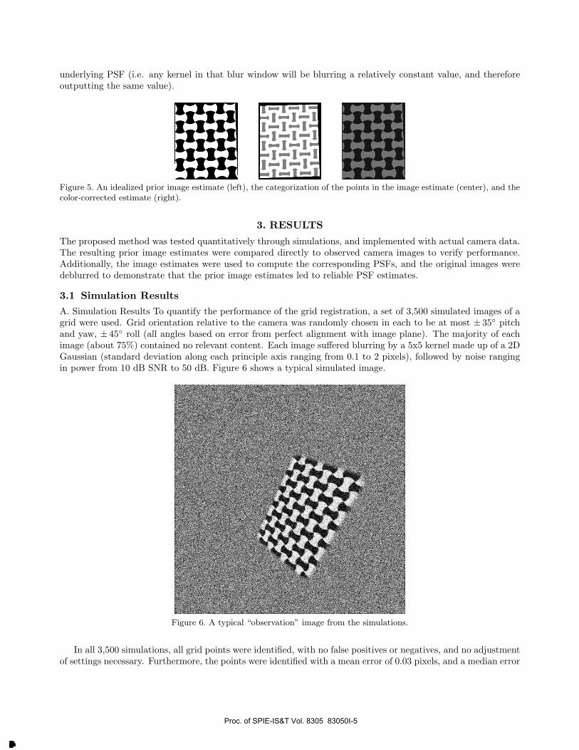
underlying PSF (i.e. any kernel in that blur window will be blurring a relatively constant value, and thereforeoutputting the same value).

Figure 5. An idealized prior image estimate (left), the categorization of the points in the image estimate (center), and thecolor-corrected estimate (right).

3. RESULTS

The proposed method was tested quantitatively through simulations, and implemented with actual camera data.The resulting prior image estimates were compared directly to observed camera images to verify performance.Additionally, the image estimates were used to compute the corresponding PSFs, and the original images weredeblurred to demonstrate that the prior image estimates led to reliable PSF estimates.

3.1 Simulation Results

A. Simulation Results To quantify the performance of the grid registration, a set of 3,500 simulated images of agrid were used. Grid orientation relative to the camera was randomly chosen in each to be at most ± 35◦ pitchand yaw, ± 45◦ roll (all angles based on error from perfect alignment with image plane). The majority of eachimage (about 75%) contained no relevant content. Each image suffered blurring by a 5x5 kernel made up of a 2DGaussian (standard deviation along each principle axis ranging from 0.1 to 2 pixels), followed by noise rangingin power from 10 dB SNR to 50 dB. Figure 6 shows a typical simulated image.

Figure 6. A typical “observation” image from the simulations.

In all 3,500 simulations, all grid points were identified, with no false positives or negatives, and no adjustmentof settings necessary. Furthermore, the points were identified with a mean error of 0.03 pixels, and a median error



of 0.12 pixels. We also looked at the SNR of the prior image estimate (where noise was defined as the pointwisedifference from the ground truth); the SNR of the estimate was on par with a realistically noisy, unblurred image,and showed little dependence on noise level, intensity of blurring, or grid alignment (Fig. 7).

Figure 7. The resulting prior SNRs, for a range of noise strengths (left), of blurring intensities (center), and of gridrotations (right).

3.2 Prior Image Estimate Results

The algorithm was used on a series of 6.0 megapixel images taken with a Nikon D70 in RAW format (linearcamera response function, with no compression). Figure 8 shows a cropped form of one such image, with a testgrid located 5 feet from the camera, a focal length of 18 mm and exposure of f/3.5. The quality of output fromeach of over 300 images was qualitatively verified by the user, but the algorithm did not require any user inputbeyond the estimated size of the blur kernel.

Figure 8. The cropped, blurry observed image (left), the light-corrected prior image estimate (center), and the two overlaidfor comparison (right).

No apparent errors were detected, even in images containing large global but low local contrast, and imagescontaining almost all superfluous image content.

3.3 PSF Estimate and Deblurring Results

In order to verify that the prior image estimate is sufficiently accurate to predict the underlying PSF, a PSFestimate is computed using a technique similar to Kee.9 The PSF estimation algorithm is modified to notinclude a smoothness prior, in which case the PSF estimate is the result of a constrained linear least-squaresoptimization (equivalently, the maximum-likelihood estimate of the PSF). The PSF estimate results from theproposed prior image estimates are compared against the results from prior image estimates which assume onlyan affine (as opposed to a projective) geometric transformation, and spatially-invariant affine color correction(Fig. 9). Although no smoothness prior is imposed in the PSF estimation, one would expect (and indeed getwith the proposed prior image estimate) a smooth, unimodal PSF.



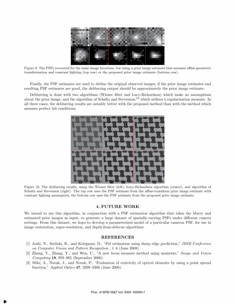
Figure 9. The PSFs recovered for the same image locations, but using a prior image estimate that assumes affine geometrictransformation and constant lighting (top row) or the proposed prior image estimate (bottom row).

Finally, the PSF estimates are used to deblur the original observed images; if the prior image estimates andresulting PSF estimates are good, the deblurring output should be approximately the prior image estimate.

Deblurring is done with two algorithms (Wiener filter and Lucy-Richardson) which make no assumptionsabout the prior image, and the algorithm of Schultz and Stevenson,10 which utilizes a regularization measure. Inall three cases, the deblurring results are notably better with the proposed method than with the method whichassumes perfect lab conditions:

Figure 10. The deblurring results, using the Wiener filter (left), Lucy-Richardson algorithm (center), and algorithm ofSchultz and Stevenson (right). The top row uses the PSF estimate from the affine-transform prior image estimate withconstant lighting assumption, the bottom row uses the PSF estimate from the proposed prior image estimate.

4. FUTURE WORK

We intend to use this algorithm, in conjunction with a PSF estimation algorithm that takes the blurry andestimated prior images as input, to generate a large dataset of spatially-varying PSFs under different camerasettings. From this dataset, we hope to develop a parameterized model of a particular cameras PSF, for use inimage restoration, super-resolution, and depth-from-defocus algorithms.

REFERENCES

[1] Joshi, N., Szeliski, R., and Kriegman, D., “Psf estimation using sharp edge prediction,” IEEE Conferenceon Computer Vision and Pattern Recognition , 1–8 (June 2008).

[2] Zhang, Y., Zhang, Y., and Wen, C., “A new focus measure method using moments,” Image and VisionComputing 18, 959–965 (September 2000).

[3] Miks, A., Novak, J., and Novak, P., “Evaluation of centricity of optical elements by using a point spreadfunction,” Applied Optics 47, 3299–3306 (June 2008).



[4] Shan, Q., Jia, J., and Agarwala, A., “High-quality motion deblurring from a single image,” ACM Transac-tions on Graphics 27, 1–10 (August 2008).

[5] Dougherty, G. and Kawaf, Z., “The point spread function revisited: Image restoration using 2-d deconvolu-tion,” Radiography 7, 255–262 (November 2001).

[6] Nakashima, P. and Johnson, A., “Measuring the psf from aperture images of arbitrary shape - an algorithm,”Ultramicroscopy 94, 135–148 (March 2003).

[7] Mikolajczyk, K. and Schmid, C., “Scale & affine invariant interest point detectors,” International Journalof Computer Vision 60, 63–86 (October 2004).

[8] Hartley, R. and Zisserman, A., [Multiple View Geometry in Computer Vision ], Cambridge University Press(2000).

[9] Kee, E., Paris, S., Chen, S., and Wang, J., “Modeling and removing spatially-varying optical blur,” in [IEEEInternational Conference on Computational Photography ], (2011).

[10] Shultz, R. and Stevenson, R., “A bayesian approach to image expansion for improved definition,” in [IEEETrans. on Image Processing ], 3(3), 233–242 (1994).



Robust Grid Registration for Non-Blind PSF Estimation Grid Registration for Non-Blind PSF Estimation...

Documents

Transcript of Robust Grid Registration for Non-Blind PSF Estimation Grid Registration for Non-Blind PSF Estimation...