Robust detection of dynamic community structure in networksmason/papers/dani-chaos-final.pdf ·...

Robust detection of dynamic community structure in networksDanielle S. Bassett, Mason A. Porter, Nicholas F. Wymbs, Scott T. Grafton, Jean M. Carlson et al. Citation: Chaos 23, 013142 (2013); doi: 10.1063/1.4790830 View online: http://dx.doi.org/10.1063/1.4790830 View Table of Contents: http://chaos.aip.org/resource/1/CHAOEH/v23/i1 Published by the American Institute of Physics. Related ArticlesTemporal dynamics and impact of event interactions in cyber-social populations Chaos 23, 013131 (2013) Topology identification of uncertain nonlinearly coupled complex networks with delays based on anticipatorysynchronization Chaos 23, 013127 (2013) Multi-stage complex contagions Chaos 23, 013124 (2013) Nucleation pathways on complex networks Chaos 23, 013112 (2013) Adaptive synchronization and pinning control of colored networks Chaos 22, 043137 (2012) Additional information on ChaosJournal Homepage: http://chaos.aip.org/ Journal Information: http://chaos.aip.org/about/about_the_journal Top downloads: http://chaos.aip.org/features/most_downloaded Information for Authors: http://chaos.aip.org/authors

Downloaded 18 Mar 2013 to 128.146.70.188. Redistribution subject to AIP license or copyright; see http://chaos.aip.org/about/rights_and_permissions

http://chaos.aip.org/?ver=pdfcov

http://aipadvances.aip.org?ver=pdfcov

http://chaos.aip.org/search?sortby=newestdate&q=&searchzone=2&searchtype=searchin&faceted=faceted&key=AIP_ALL&possible1=Danielle S. Bassett&possible1zone=author&alias=&displayid=AIP&ver=pdfcov

http://chaos.aip.org/search?sortby=newestdate&q=&searchzone=2&searchtype=searchin&faceted=faceted&key=AIP_ALL&possible1=Mason A. Porter&possible1zone=author&alias=&displayid=AIP&ver=pdfcov

http://chaos.aip.org/search?sortby=newestdate&q=&searchzone=2&searchtype=searchin&faceted=faceted&key=AIP_ALL&possible1=Nicholas F. Wymbs&possible1zone=author&alias=&displayid=AIP&ver=pdfcov

http://chaos.aip.org/search?sortby=newestdate&q=&searchzone=2&searchtype=searchin&faceted=faceted&key=AIP_ALL&possible1=Scott T. Grafton&possible1zone=author&alias=&displayid=AIP&ver=pdfcov

http://chaos.aip.org/search?sortby=newestdate&q=&searchzone=2&searchtype=searchin&faceted=faceted&key=AIP_ALL&possible1=Jean M. Carlson&possible1zone=author&alias=&displayid=AIP&ver=pdfcov


http://link.aip.org/link/doi/10.1063/1.4790830?ver=pdfcov

http://chaos.aip.org/resource/1/CHAOEH/v23/i1?ver=pdfcov

http://www.aip.org/?ver=pdfcov







http://chaos.aip.org/about/about_the_journal?ver=pdfcov

http://chaos.aip.org/features/most_downloaded?ver=pdfcov

http://chaos.aip.org/authors?ver=pdfcov

Robust detection of dynamic community structure in networks

Danielle S. Bassett,1,2,a) Mason A. Porter,3,4 Nicholas F. Wymbs,5 Scott T. Grafton,5

Jean M. Carlson,1 and Peter J. Mucha6,7

1Department of Physics, University of California, Santa Barbara, California 93106, USA2Sage Center for the Study of the Mind, University of California, Santa Barbara, California 93106, USA3Oxford Centre for Industrial and Applied Mathematics, Mathematical Institute, University of Oxford,Oxford OX1 3LB, United Kingdom4CABDyN Complexity Centre, University of Oxford, Oxford OX1 1HP, United Kingdom5Department of Psychological & Brain Sciences and UCSB Brain Imaging Center, University of California,Santa Barbara, California 93106, USA6Department of Mathematics, Carolina Center for Interdisciplinary Applied Mathematics,University of North Carolina, Chapel Hill, North Carolina 27599, USA7Institute for Advanced Materials, Nanoscience & Technology, University of North Carolina,Chapel Hill, North Carolina 27599, USA

(Received 19 June 2012; accepted 8 January 2013; published online 18 March 2013)

We describe techniques for the robust detection of community structure in some classes of time-

dependent networks. Specifically, we consider the use of statistical null models for facilitating

the principled identification of structural modules in semi-decomposable systems. Null models

play an important role both in the optimization of quality functions such as modularity and in the

subsequent assessment of the statistical validity of identified community structure. We examine

the sensitivity of such methods to model parameters and show how comparisons to null models

can help identify system scales. By considering a large number of optimizations, we quantify the

variance of network diagnostics over optimizations (“optimization variance”) and over

randomizations of network structure (“randomization variance”). Because the modularity quality

function typically has a large number of nearly degenerate local optima for networks constructed

using real data, we develop a method to construct representative partitions that uses a null model

to correct for statistical noise in sets of partitions. To illustrate our results, we employ ensembles

of time-dependent networks extracted from both nonlinear oscillators and empirical neuroscience

data. VC 2013 American Institute of Physics. [http://dx.doi.org/10.1063/1.4790830]

Many social, physical, technological, and biological systems

can be modeled as networks composed of numerous inter-

acting parts.1

As an increasing amount of time-resolved

data has become available, it has become increasingly im-

portant to develop methods to quantify and characterize

dynamic properties of temporal networks.2 Generalizing the

study of static networks, which are typically represented

using graphs, to temporal networks entails the considera-

tion of nodes (representing entities) and/or edges (repre-

senting ties between entities) that vary in time. As one

considers data with more complicated structures, the

appropriate network analyses must become increasingly

nuanced. In the present paper, we discuss methods for

algorithmic detection of dense clusters of nodes (i.e., com-

munities) by optimizing quality functions on multilayer

network representations of temporal networks.3,4

We

emphasize the development and analysis of different types

of null-model networks, whose appropriateness depends on

the structure of the networks one is studying as well as the

construction of representative partitions that take advant-

age of a multilayer network framework. To illustrate our

ideas, we use ensembles of time-dependent networks from

the human brain and human behavior.

I. INTRODUCTION

Myriad systems have components whose interactions (or

the components themselves) change as a function of time.

Many of these systems can be investigated using the frame-

work of temporal networks, which consist of sets of nodes

and/or edges that vary in time.2 The formalism of temporal

networks is convenient for studying data drawn from areas

such as person-to-person communication (e.g., via mobile

phones5,6), one-to-many information dissemination (such as

Twitter networks7), cell biology, distributed computing,

infrastructure networks, neural and brain networks, and eco-

logical networks.2 Important phenomena that can be studied

in this framework include network constraints on gang and

criminal activity,8,9 political processes,10,11 human brain

function,4,12 human behavior,13 and financial structures.14,15

Time-dependent complex systems can have densely con-

nected components in the form of cohesive groups of nodes

known as “communities” (see Fig. 1), which can be related to

a system’s functional modules.16,17 A wide variety of

a)Author to whom correspondence should be addressed. Electronic mail:

[email protected].

1054-1500/2013/23(1)/013142/16/$30.00 VC 2013 American Institute of Physics23, 013142-1

CHAOS 23, 013142 (2013)


http://dx.doi.org/10.1063/1.4790830

http://dx.doi.org/10.1063/1.4790830

mailto:[email protected]

http://crossmark.crossref.org/dialog/?doi=10.1063/1.4790830&domain=pdf&date_stamp=2013-03-18

clustering techniques have been developed to identify com-

munities, and they have yielded insights in the study of the

committee structure in the United States Congress,18 func-

tional groups in protein interaction networks,19 functional

modules in brain networks,4 and more. A particularly success-

ful technique for identifying communities in networks16,20 is

optimization of a quality function known as “modularity,”21

which recently has been generalized for detecting commun-

ities in time-dependent and multiplex networks.3

Modularity optimization allows one to algorithmically

partition a network’s nodes into communities such that the

total connection strength within groups of the partition is more

than would be expected in some null model. However, modu-

larity optimization always yields a network partition (into a set

of communities) as an output whether or not a given network

truly contains modular structure. Therefore, application of sub-

sequent diagnostics to a network partition is potentially mean-

ingless without some comparison to benchmark or null-model

networks. That is, it is important to establish whether the parti-

tion(s) obtained appear to represent meaningful community

structures within the network data or whether they might have

reasonably arisen at random. Moreover, robust assessment of

network organization depends fundamentally on the develop-

ment of statistical techniques to compare structures in a net-

work derived from real data to those in appropriate models

(see, e.g., Ref. 22). Indeed, as the constraints in null models

and network benchmarks become more stringent, it can

become possible to make stronger claims when interpreting

organizational structures such as community structure.

In the present paper, we examine null models in time-

dependent networks and investigate their use in the algorithmic

detection of cohesive, dynamic communities in such networks

(see Fig. 2). Indeed, community detection in temporal net-

works necessitates the development of null models that are

appropriate for such networks. Such null models can help pro-

vide bases of comparison at various stages of the community-

detection process, and they can thereby facilitate the principled

identification of dynamic structure in networks. Indeed, the im-

portance of developing null models extends beyond commu-

nity detection, as such models make it possible to obtain

statistically significant estimates of network diagnostics.

Our dynamic network null models fall into two catego-

ries: optimization null models, which we use in the identifi-

cation of community structure; and post-optimization null

models, which we use to examine the identified community

structure. We describe how these null models can be selected

in a manner appropriate to known features of a network’s

construction, identify potentially interesting network scales

by determining values of interest for structural and temporal

resolution parameters, and inform the choice of representa-

tive partitions of a network into communities.

II. METHODS

A. Community detection

Community-detection algorithms provide ways to decom-

pose a network into dense groups of nodes called “modules”

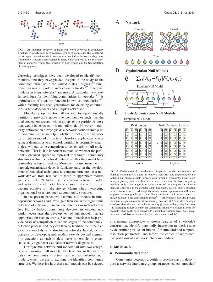
FIG. 1. An important property of many real-world networks is community

structure, in which there exist cohesive groups of nodes such that a network

has stronger connections within such groups than it does between such groups.

Community structure often changes in time, which can lead to the rearrange-

ment of cohesive groups, the formation of new groups, and the fragmentation

of existing groups.

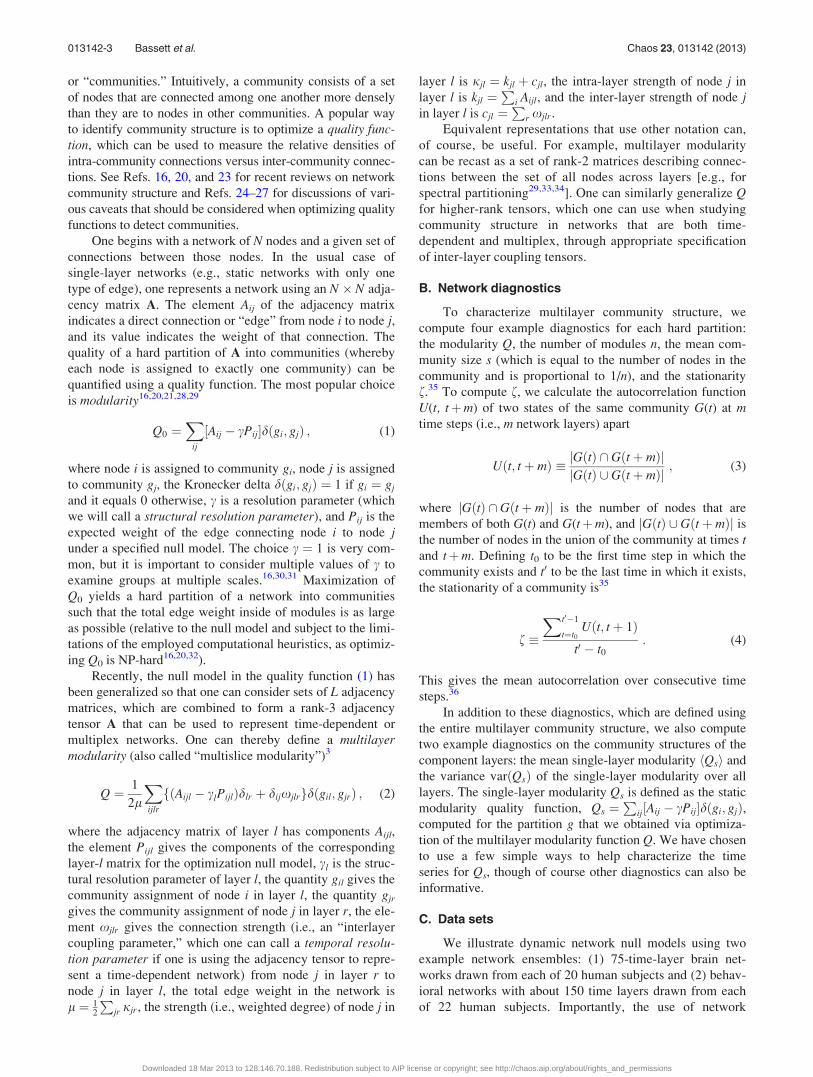
FIG. 2. Methodological considerations important in the investigation of

dynamic community structure in temporal networks. (A) Depending on the

system under study, a single network layer (which is represented using an or-

dinary adjacency matrix with an extra index to indicate the layer) might by

definition only allow edges from some subset of the complete set of node

pairs, as is the case in the depicted chain-like graph. We call such a situation

partial connectivity. (B) Although the most common optimization null model

employs random graphs (e.g., the Newman-Girvan null model, which is

closely related to the configuration model1,16), other models can also provide

important insights into network community structure. (C) After determining a

set of partitions that maximize the modularity Q (or a similar quality function),

it is interesting to test whether the community structure is different from, for

example, what would be expected with a scrambling of time layers (i.e., a tem-

poral null model) or node identities (i.e., a nodal null model).4

013142-2 Bassett et al. Chaos 23, 013142 (2013)


or “communities.” Intuitively, a community consists of a set

of nodes that are connected among one another more densely

than they are to nodes in other communities. A popular way

to identify community structure is to optimize a quality func-tion, which can be used to measure the relative densities of

intra-community connections versus inter-community connec-

tions. See Refs. 16, 20, and 23 for recent reviews on network

community structure and Refs. 24–27 for discussions of vari-

ous caveats that should be considered when optimizing quality

functions to detect communities.

One begins with a network of N nodes and a given set of

connections between those nodes. In the usual case of

single-layer networks (e.g., static networks with only one

type of edge), one represents a network using an N � N adja-

cency matrix A. The element Aij of the adjacency matrix

indicates a direct connection or “edge” from node i to node j,and its value indicates the weight of that connection. The

quality of a hard partition of A into communities (whereby

each node is assigned to exactly one community) can be

quantified using a quality function. The most popular choice

is modularity16,20,21,28,29

Q0 ¼X

ij

½Aij � cPij�dðgi; gjÞ ; (1)

where node i is assigned to community gi, node j is assigned

to community gj, the Kronecker delta dðgi; gjÞ ¼ 1 if gi ¼ gj

and it equals 0 otherwise, c is a resolution parameter (which

we will call a structural resolution parameter), and Pij is the

expected weight of the edge connecting node i to node junder a specified null model. The choice c ¼ 1 is very com-

mon, but it is important to consider multiple values of c to

examine groups at multiple scales.16,30,31 Maximization of

Q0 yields a hard partition of a network into communities

such that the total edge weight inside of modules is as large

as possible (relative to the null model and subject to the limi-

tations of the employed computational heuristics, as optimiz-

ing Q0 is NP-hard16,20,32).

Recently, the null model in the quality function (1) has

been generalized so that one can consider sets of L adjacency

matrices, which are combined to form a rank-3 adjacency

tensor A that can be used to represent time-dependent or

multiplex networks. One can thereby define a multilayermodularity (also called “multislice modularity”)3

Q ¼ 1

2l

Xijlr

fðAijl � clPijlÞdlr þ dijxjlrgdðgil; gjrÞ ; (2)

where the adjacency matrix of layer l has components Aijl,

the element Pijl gives the components of the corresponding

layer-l matrix for the optimization null model, cl is the struc-

tural resolution parameter of layer l, the quantity gil gives the

community assignment of node i in layer l, the quantity gjr

gives the community assignment of node j in layer r, the ele-

ment xjlr gives the connection strength (i.e., an “interlayer

coupling parameter,” which one can call a temporal resolu-tion parameter if one is using the adjacency tensor to repre-

sent a time-dependent network) from node j in layer r to

node j in layer l, the total edge weight in the network is

l ¼ 12

Pjr jjr, the strength (i.e., weighted degree) of node j in

layer l is jjl ¼ kjl þ cjl, the intra-layer strength of node j in

layer l is kjl ¼P

i Aijl, and the inter-layer strength of node jin layer l is cjl ¼

Pr xjlr.

Equivalent representations that use other notation can,

of course, be useful. For example, multilayer modularity

can be recast as a set of rank-2 matrices describing connec-

tions between the set of all nodes across layers [e.g., for

spectral partitioning29,33,34]. One can similarly generalize Qfor higher-rank tensors, which one can use when studying

community structure in networks that are both time-

dependent and multiplex, through appropriate specification

of inter-layer coupling tensors.

B. Network diagnostics

To characterize multilayer community structure, we

compute four example diagnostics for each hard partition:

the modularity Q, the number of modules n, the mean com-

munity size s (which is equal to the number of nodes in the

community and is proportional to 1/n), and the stationarity

f.35 To compute f, we calculate the autocorrelation function

U(t, tþm) of two states of the same community G(t) at mtime steps (i.e., m network layers) apart

Uðt; tþ mÞ � jGðtÞ \ Gðtþ mÞjjGðtÞ [ Gðtþ mÞj ; (3)

where jGðtÞ \ Gðtþ mÞj is the number of nodes that are

members of both G(t) and G(tþm), and jGðtÞ [ Gðtþ mÞj isthe number of nodes in the union of the community at times tand tþm. Defining t0 to be the first time step in which the

community exists and t0 to be the last time in which it exists,

the stationarity of a community is35

f �

Xt0�1

t¼t0Uðt; tþ 1Þ

t0 � t0

: (4)

This gives the mean autocorrelation over consecutive time

steps.36

In addition to these diagnostics, which are defined using

the entire multilayer community structure, we also compute

two example diagnostics on the community structures of the

component layers: the mean single-layer modularity hQsi and

the variance varðQsÞ of the single-layer modularity over all

layers. The single-layer modularity Qs is defined as the static

modularity quality function, Qs ¼P

ij½Aij � cPij�dðgi; gjÞ,computed for the partition g that we obtained via optimiza-

tion of the multilayer modularity function Q. We have chosen

to use a few simple ways to help characterize the time

series for Qs, though of course other diagnostics can also be

informative.

C. Data sets

We illustrate dynamic network null models using two

example network ensembles: (1) 75-time-layer brain net-

works drawn from each of 20 human subjects and (2) behav-

ioral networks with about 150 time layers drawn from each

of 22 human subjects. Importantly, the use of network



ensembles makes it possible to examine robust structure (and

also its variance) over multiple network instantiations. We

have previously examined both data sets in the context of

neuroscientific questions.4,13 In this paper, we use them as il-

lustrative examples for the consideration of methodological

issues in the detection of dynamic communities in temporal

networks.

These two data sets, which provide examples of differ-

ent types of network data, illustrate a variety of issues in net-

work construction: (1) node and edge definitions, (2)

complete versus partial connectivity, (3) ordered versus cate-

gorical nodes, and (4) confidence in edge weights. In many

fields, determining the definition of nodes and edges is itself

an active area of investigation.37 See, for example, several

recent papers that address such questions in the context of

large-scale human brain networks38–43 and in networks more

generally.44 Another important issue is whether to examine a

given adjacency matrix in an exploratory manner or to

impose structure on it based on a priori knowledge. For

example, when nodes are categorical, one might represent

their relations using a fully connected network and then iden-

tify communities of any group of nodes. However, when

nodes are ordered—and particularly when they are in a chain

of weighted nearest-neighbor connections—one expects

communities to group neighboring nodes in sequence, as typ-

ical community-detection methods are unlikely to yield

many out-of-sequence jumps in community assignment. The

issue of confidence in the estimation of edge weights is also

very important, as it can prompt an investigator to delete

edges from a network when their statistical validity is ques-

tionable. A closely related issue is how to deal with known

or expected missing data, which can affect either the pres-

ence or absence of nodes themselves or the weights of

edges.45–48

D. Data set 1: Brain networks

Our first data set contains categorical nodes with partial

connectivity and variable confidence in edge weights. The

nodes remain unchanged in time, and edge weights are based

on covariance of node properties. This covariance structure

is non-local in the sense that weights exist between both

topologically neighboring nodes and topologically distant

nodes.49,50 This property has been linked in other dynamical

systems to behaviors such as chimera states, in which coher-

ent and incoherent regions coexist.51–53 Another interesting

feature of this data set is that it is drawn from an experimen-

tal measurement with high spatial resolution (on the order of

centimeters) but relatively poor temporal resolution (on the

order of seconds).

As described in more detail in Ref. 4, we construct an

ensemble of networks (20 individuals over 3 experiments,

which yields 60 multilayer networks) that represent the func-

tional connectivity between large regions of the human brain.

In these networks, N¼ 112 centimeter-scale, anatomically

distinct brain regions are our (categorical) network nodes.

We study the temporal interaction of these nodes—such

interactions are thought to underly cognitive function—by

first measuring their activity every 2 s during simple finger

movements using functional magnetic resonance imaging

(fMRI). We cut these regional time series into time slices

(which yield layers in the multilayer network) of roughly

3-min duration. Each such layer corresponds to a time series

whose length is 80 units.

To estimate the interactions (i.e., edge weights) between

nodes, we calculate a measure of statistical similarity

between regional activity profiles.54 Using a wavelet trans-

form, we extract frequency-specific activity from each time

series in the range 0.06–0.12 Hz. For each time layer l and

each pair of regions i and j, we define the weight of an edge

connecting region i to region j using the coherence between

the wavelet-coefficient time series in each region, and these

weights form the elements of a weighted, undirected tempo-

ral network W with components Wijl ¼ Wjil. The magnitude-squared coherence Gij between time series i and j is a func-

tion of frequency. It is defined by the equation

Gijðf Þ ¼jFijðf Þj2

Fiiðf ÞFjjðf Þ; (5)

where Fiiðf Þ and Fjjðf Þ are the power spectral density func-

tions of i and j, respectively, and Fijðf Þ is the cross-power

spectral density function of i and j. We let Hij denote the

mean of Gijðf Þ over the frequency band of interest, and the

weight of edge Wijl is equal to Hij computed for layer l.We use a false-discovery rate correction55 to threshold

connections whose coherence values are not significantly

greater than that expected at random. This yields a multilayer

network A with components Aijl (i.e., a rank-3 adjacency ten-

sor). The nonzero entries in A retain their weights. We cou-

ple the layers of A to one another with temporal resolution

parameters of weight xjlr between node j in layer r and node

j in layer l. In this paper, we let xjlr � x 2 ½0:1; 40� be iden-

tical between each node j in a given layer and itself in

nearest-neighbor layers. (In all other cases, xjlr ¼ 0.)

In Fig. 3(a), we show an example time layer from A for

a single subject in this experimental data. In this example,

the statistical threshold is evinced by the set of matrix ele-

ments set to 0. Because brain network nodes are categorical,

one can apply community detection algorithms in these sit-

uations to identify communities composed of any set of

nodes. (Note that the same node from different times can be

assigned to the same community even if the node is assigned

to other communities at intervening times.) One biological

interpretation of network communities in brain networks is

that they represent groups of nodes that serve distinct cogni-

tive functions (e.g., vision, memory, etc.) that can vary in

time.12,56

E. Data set 2: Behavioral networks

Our second data set contains ordered nodes that remain

unchanged in time. The network topology in this case is

highly constrained, as edges are only present between con-

secutive nodes. (We call this “nearest-neighbor” coupling.)

Another interesting feature of this data set is that the number

of time slices is an order of magnitude larger than the num-

ber of nodes in a slice.



As described in more detail in Ref. 13, we construct an

ensemble of 66 behavioral networks from 22 individuals and

3 experimental conditions. These networks represent a set of

finger movements in the same simple motor learning experi-

ment from which we constructed the brain networks in data

set 1. Subjects were instructed to press a sequence of buttons

corresponding to a sequence of 12 pseudo-musical notes

shown to them on a screen.

Each node represents an interval between consecutive

button presses. A single network layer consists of N¼ 11

nodes (i.e., there is one interval between each pair of notes),

which are connected in a chain via weighted, undirected

edges. In Ref. 13, we examined the phenomenon of motor

“chunking,” which is a fascinating but poorly understood

phenomenon in which groups of movements are made with

similar inter-movement durations. (This is similar to remem-

bering a phone number in groups of a few digits or grouping

notes together as one masters how to play a song.) For each

experimental trial l and each pair of inter-movement inter-

vals i and j, we define the weight of an edge connecting

inter-movement i to inter-movement j as the normalized sim-

ilarity in inter-movement durations. The normalized similar-ity between nodes i and j is defined as

qijl ¼�dl � dijl

�dl; (6)

where dijl is the absolute value of the difference of lengths of

the ith and jth inter-movement time intervals in trial l and �dl

is the maximum value of dijl in trial l. These weights yield

the elements Wijl of a weighted, undirected multilayer net-

work W. Because finger movements occur in series, inter-

movement i is connected in time to inter-movement i 6 1 but

not to any other inter-movements iþ n for jnj 6¼ 1.

To encode this conceptual relationship as a network, we

set all non-contiguous connections in W to 0 and thereby

construct a weighted, undirected chain network A. In Fig.

3(b), we show an example trial layer from A for a single sub-

ject in this experimental data. We couple layers of A to one

another with weight xjlr, which gives the connection strength

between node j in experimental trial r and node j in trial l. In

a given instantiation of the network, we again let xjlr � x 2½0:1; 40� be identical for all nodes j for all connections

between nearest-neighbor layers. (Again, xjlr ¼ 0 in all other

cases.) Because inter-movement nodes are ordered, one can

apply community-detection algorithms to identify commun-

ities of nodes in sequence. Each community represents a

motor “chunk.”

III. RESULTS

A. Modularity-optimization null models

After constructing a multilayer network A with elements

Aijl, it is necessary to select an optimization null model P in

Eq. (2). The most common modularity-optimization null

model used in undirected, single-layer networks is the

Newman-Girvan null model16,20,21,28,29

Pij ¼kikj

2m; (7)

where ki ¼P

j Aij is the strength of node i and m ¼ 12

Pij Aij.

The definition (7) can be extended to multilayer networks

using

Pijl ¼kilkjl

2ml; (8)

where kil ¼P

j Aijl is the strength of node i in layer l and

ml ¼ 12

Pij Aijl. Optimization of Q using the null model (8)

identifies partitions of a network into groups that have more

connections (in the case of binary networks) or higher con-

nection densities (in the case of weighted networks) than

would be expected for the distribution of connections (or

connection densities) expected in a null model. We use the

notation Al for the layer-l adjacency matrix composed of ele-

ments Aijl and the notation Pl to denote the layer-l null-

model matrix with elements Pijl. See Fig. 4(a) for an example

layer Al from a multilayer behavioral network and Fig. 4(b)

for an example instantiation of the Newman-Girvan null

model Pl.

1. Optimization null models for ordered nodenetworks

The Newman-Girvan null model is particularly useful

for networks with categorical nodes, in which a connection

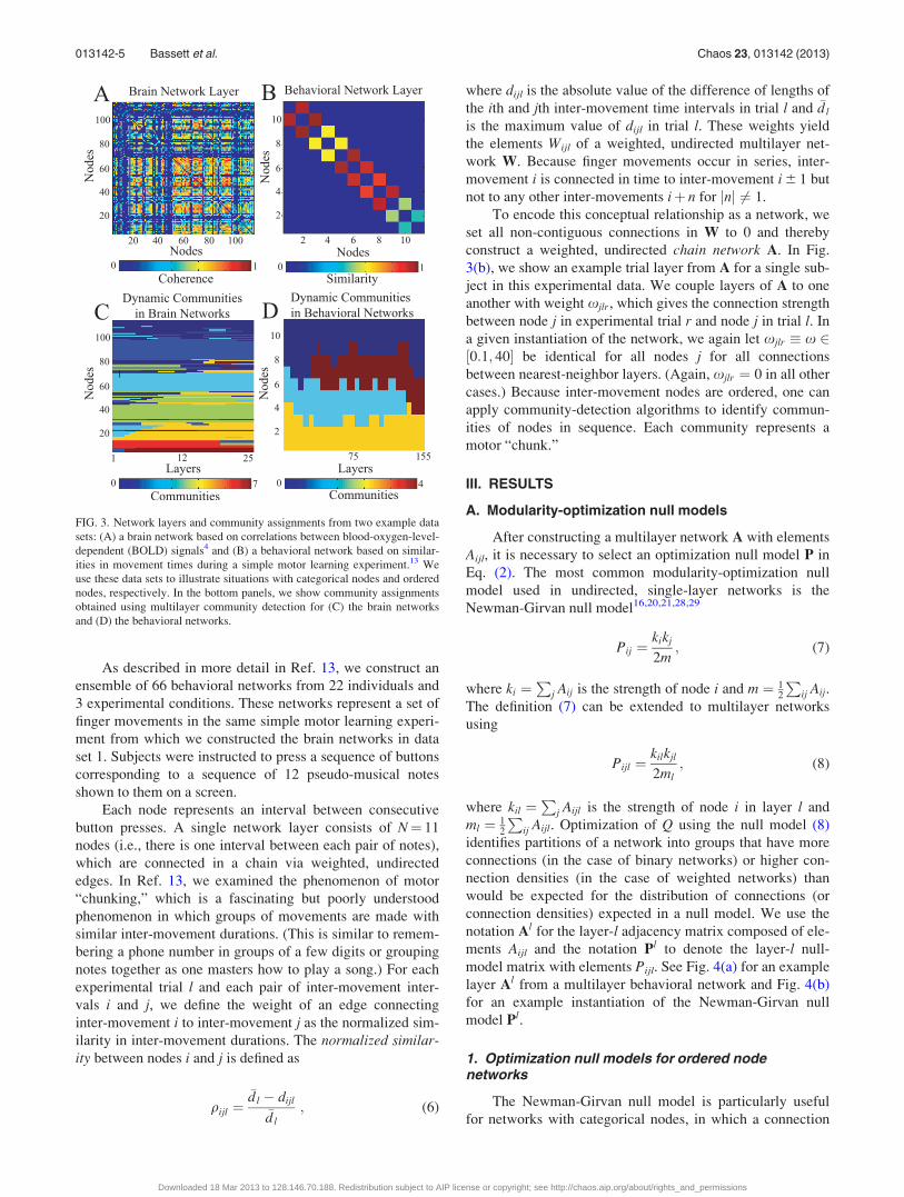
FIG. 3. Network layers and community assignments from two example data

sets: (A) a brain network based on correlations between blood-oxygen-level-

dependent (BOLD) signals4 and (B) a behavioral network based on similar-

ities in movement times during a simple motor learning experiment.13 We

use these data sets to illustrate situations with categorical nodes and ordered

nodes, respectively. In the bottom panels, we show community assignments

obtained using multilayer community detection for (C) the brain networks

and (D) the behavioral networks.



between any pair of nodes can occur in theory. However,

when using a chain network of ordered nodes, it is useful to

consider alternative null models. For example, in a network

represented by an adjacency matrix A0, one can define

Pij ¼ qA0ij ; (9)

where q is the mean edge weight of the chain network and

A0 is the binarized version of A, in which nonzero elements

of A are set to 1 and zero-valued elements remain unaltered.

Such a null model can also be defined for a multilayer net-

work that is represented by a rank-3 adjacency tensor A. One

can construct a null model P with components

Pijl ¼ qlA0ijl ; (10)

where ql is the mean edge weight in layer l and A0 is the

binarized version of A. The optimization of Q using this null

model identifies partitions of a network whose communities

have a larger strength than the mean. See Fig. 4(c) for an

example of this chain null model Pl for the behavioral net-

work layer shown in Fig. 4(a).

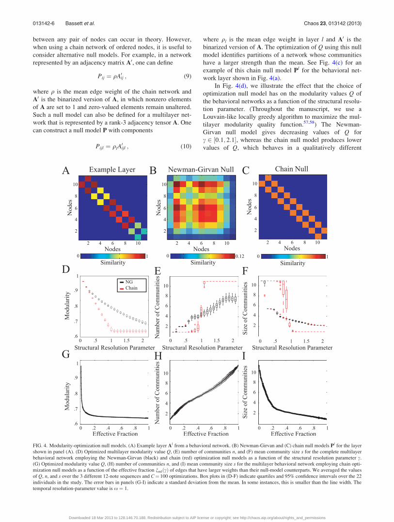
In Fig. 4(d), we illustrate the effect that the choice of

optimization null model has on the modularity values Q of

the behavioral networks as a function of the structural resolu-

tion parameter. (Throughout the manuscript, we use a

Louvain-like locally greedy algorithm to maximize the mul-

tilayer modularity quality function.57,58) The Newman-

Girvan null model gives decreasing values of Q for

c 2 ½0:1; 2:1�, whereas the chain null model produces lower

values of Q, which behaves in a qualitatively different

FIG. 4. Modularity-optimization null models. (A) Example layer Al from a behavioral network. (B) Newman-Girvan and (C) chain null models Pl for the layer

shown in panel (A). (D) Optimized multilayer modularity value Q, (E) number of communities n, and (F) mean community size s for the complete multilayer

behavioral network employing the Newman-Girvan (black) and chain (red) optimization null models as a function of the structural resolution parameter c.

(G) Optimized modularity value Q, (H) number of communities n, and (I) mean community size s for the multilayer behavioral network employing chain opti-

mization null models as a function of the effective fraction nmlðcÞ of edges that have larger weights than their null-model counterparts. We averaged the values

of Q, n, and s over the 3 different 12-note sequences and C¼ 100 optimizations. Box plots in (D-F) indicate quartiles and 95% confidence intervals over the 22

individuals in the study. The error bars in panels (G-I) indicate a standard deviation from the mean. In some instances, this is smaller than the line width. The

temporal resolution-parameter value is x ¼ 1.



manner for c < 1 versus c > 1. To help understand this fea-

ture, we plot the number and mean size of communities as a

function of c in Figs. 4(e) and 4(f). As c is increased, the

Newman-Girvan null model yields network partitions that

contain progressively more communities (with progressively

smaller mean size). The number of communities that we

obtain in partitions using the chain null model also increases

with c, but it does so less gradually. For c� 1, one obtains a

network partition consisting of a single community of size

Nl ¼ 11; for c� 1, each node is instead placed in its own

community. For c ¼ 1, nodes are assigned to several com-

munities whose constituents vary with time (see, for exam-

ple, Fig. 3(d)).

The above results highlight the sensitivity of network

diagnostics such as Q, n, and s to the choice of an optimiza-

tion null model. It is important to consider this type of sensi-

tivity in the light of other known issues, such as the extreme

near-degeneracy of quality functions like modularity.24

Importantly, the use of the chain null model provides a clear

delineation of network behavior in this example into three

regimes as a function of c: a single community with variable

Q (low c), a variable number of communities as Q reaches a

minimum value (c � 1), and a set of singleton communities

with minimum Q (high c). This illustrates that it is crucial to

consider a null model appropriate for a given network, as it

can provide more interpretable results than just using the

usual choices (such as the Newman-Girvan null model).

The structural resolution parameter c can be transformed

so that it measures the effective fraction of edges nðcÞ that

have larger weights than their null-model counterparts.31

One can define a generalization of n to multilayer networks,

which allows one to examine the behavior of the chain null

model near c ¼ 1 in more detail. For each layer l, we define

a matrix XlðcÞ with elements XijlðcÞ ¼ Aijl � cPijl, and we

then define cXðcÞ to be the number of elements of XlðcÞ that

are less than 0. We sum cXðcÞ over layers in the multilayer

network to construct cXmlðcÞ. The transformed structural reso-

lution parameter is then given by

nmlðcÞ ¼cX

mlðcÞ � cXmlðKminÞ

cXmlðKmaxÞ � cX

mlðKminÞ; (11)

where Kmin is the value of c for which the network still forms

a single community in the multilayer optimization, and Kmax

is the value of c for which the network still forms N singleton

communities in the multilayer optimization. (We use Roman

typeface in the subscripts in cXml and nml to emphasize that we

are describing multilayer objects and, in particular, that the

subscripts do not represent indices.) In Figs. 4(g)–4(i), we

report the optimized (i.e., maximized) modularity value, the

number of communities, and the mean community size as

functions of the transformed structural resolution parameter

nmlðcÞ. (Compare these plots to Figs. 4(d)–4(f).) For all three

diagnostics, the apparent transition points seem to be more

gradual as a function of nmlðcÞ than they are as a function of

c. For systems like the present one that do not exhibit a pro-

nounced, nontrivial plateau in these diagnostics as a function

of a structural resolution parameter, it might be helpful to

have a priori knowledge about the expected number or sizes

of communities (see, e.g., Ref. 13) to help guide further

investigation.

2. Optimization null models for networks derived fromtime series

Although the Newman-Girvan null model can be used in

networks with categorical nodes, such as the brain networks

in data set 1 (see Fig. 5(a)), it does not take advantage of the

fact that these networks are derived from similarities in time

series. Accordingly, we generate surrogate data to construct

two dynamic network null models for community detection

that might be particularly appropriate for networks derived

from time-series data.

First, we note that a simple null model (which we call

“Random”) for time series is to randomize the elements of

the time-series vector for each node before computing the

similarity matrix (see Fig. 5(b)).59 However, the resulting

time series do not have the mean or variance of the original

time series, and this yields a correlation- or coherence-based

network with very low edge weights. To preserve the mean,

variance, and autocorrelation function of the original time

series, we employ a surrogate-data generation method that

scrambles the phase of time series in Fourier space.60

Specifically, we assume that the linear properties of the time

series are specified by the squared amplitudes of the discrete

Fourier transform (FT)

jSðuÞj2 ¼ 1ffiffiffiffiVp

XV�1

v¼0

svei2puv=V

��2

; (12)

where sv denotes an element in a time series of length V.

(That is, V is the number of elements in the time-series vec-

tor.) We construct surrogate data by multiplying the Fourier

transform by phases chosen uniformly at random and trans-

forming back to the time domain

�sv ¼1ffiffiffiffiVp

XV�1

v¼0

eiau jSujei2pkv=V ; (13)

where au 2 ½0; 2pÞ are chosen independently and uniformly

at random.61 This method, which we call the FT surrogate(see Fig. 5(c)), has been used previously to construct covari-

ance matrices62 and to characterize networks.63 A modifica-

tion of this method, which we call the amplitude-adjustedFourier transform (AAFT) surrogate, allows one to also

retain the amplitude distribution of the original signal64 (see

Fig. 5(d)). One can alter nonlinear relationships between

time series while preserving linear relationships between

time series by applying an identical shuffling to both time se-

ries; one can alter both linear and nonlinear relationships

between time series by applying independent shufflings to

each time series.60

We demonstrate in Fig. 5(e) that, among the four null

models that we consider, the mean coherence of pairs of FT

surrogate series match that of the original data most closely.

Pairs of Random time series have the smallest mean coher-

ence, and pairs of AAFT surrogate series have the next



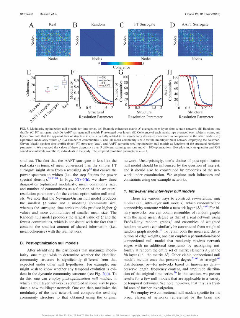
smallest. The fact that the AAFT surrogate is less like the

real data (in terms of mean coherence) than the simpler FT

surrogate might stem from a rescaling step62 that causes the

power spectrum to whiten (i.e., the step flattens the power

spectral density).65,83,84 In Figs. 5(f)–5(h), we show three

diagnostics (optimized modularity, mean community size,

and number of communities) as a function of the structural

resolution parameter c for the various optimization null mod-

els. We note that the Newman-Girvan null model produces

the smallest Q value and a middling community size,

whereas the surrogate time series models produce higher Qvalues and more communities of smaller mean size. The

Random null model produces the largest value of Q and the

fewest communities, which is consistent with the fact that it

contains the smallest amount of shared information (i.e.,

mean coherence) with the real network.

B. Post-optimization null models

After identifying the partition(s) that maximize modu-

larity, one might wish to determine whether the identified

community structure is significantly different from that

expected under other null hypotheses. For example, one

might wish to know whether any temporal evolution is evi-

dent in the dynamic community structure (see Fig. 2(c)). To

do this, one can employ post-optimization null models, in

which a multilayer network is scrambled in some way to pro-

duce a new multilayer network. One can then maximize the

modularity of the new network and compare the resulting

community structure to that obtained using the original

network. Unsurprisingly, one’s choice of post-optimization

null model should be influenced by the question of interest,

and it should also be constrained by properties of the net-

work under examination. We explore such influences and

constraints using our example networks.

1. Intra-layer and inter-layer null models

There are various ways to construct connectional nullmodels (i.e., intra-layer null models), which randomize the

connectivity structure within a network layer (Al).4,66 For bi-

nary networks, one can obtain ensembles of random graphs

with the same mean degree as that of a real network using

Erd}os-R�enyi random graphs,1 and ensembles of weighted

random networks can similarly be constructed from weighted

random graph models.67 To retain both the mean and distri-

bution of edge weights, one can employ a permutation-based

connectional null model that randomly rewires network

edges with no additional constraints by reassigning uni-

formly at random the entire set of matrix elements Aijl in the

lth layer (i.e., the matrix Al). Other viable connectional null

models include ones that preserve degree21,68 or strength69

distributions, or—for networks based on time-series data—

preserve length, frequency content, and amplitude distribu-

tion of the original time series.70 In this section, we present

results for a few null models that are applicable to a variety

of temporal networks. We note, however, that this is a fruit-

ful area of further investigation.

We employ two connectional null models specific for the

broad classes of networks represented by the brain and

FIG. 5. Modularity-optimization null models for time series. (A) Example coherence matrix Al averaged over layers from a brain network. (B) Random time

shuffle, (C) FT surrogate, and (D) AAFT surrogate null models Pl averaged over layers. (E) Coherence of each matrix type averaged over subjects, scans, and

layers. We note that the apparent lack of structure in (B) is partially related to its significantly decreased coherence in comparison to the other models. (F)

Optimized modularity values Q, (G) number of communities n, and (H) mean community size s for the multilayer brain network employing the Newman-

Girvan (black), random time-shuffle (blue), FT surrogate (gray), and AAFT surrogate (red) optimization null models as functions of the structural resolution

parameter c. We averaged the values of these diagnostics over 3 different scanning sessions and C¼ 100 optimizations. Box plots indicate quartiles and 95%

confidence intervals over the 20 individuals in the study. The temporal resolution parameter is x ¼ 1.



behavioral networks that we use as examples in this paper.

The brain networks provide an example of time-dependent

similarity networks, which are weighted and either fully con-

nected or almost fully connected.31 (The brain networks have

some 0 entries in their corresponding adjacency tensors

because we have removed edges with weights that are not

statistically significant.4) We, therefore, employ a constrained

null model that is constructed by randomly rewiring edges

while maintaining the empirical degree distribution.68 In Fig.

6(a1), we demonstrate the use of this null model to assess

dynamic community structure. Importantly, this constrained

null model can be used in principle for any binary or weighted

network, though it does not take advantage of specific struc-

ture (aside from strength distribution) that one might want to

exploit. For example, the behavioral networks have chain-like

topologies, and it is desirable to develop models that are spe-

cifically appropriate for such situations. (One can obviously

make the same argument for other specific topologies.) We,

therefore, introduce a highly constrained connectional null

model that is constructed by reassigning edge weights uni-

formly at random to existing edges. This does not change the

underlying binary topology. (That is, we preserve network to-

pology but scramble network geometry.) We demonstrate the

use of this null model in Fig. 6(b1).

In addition to intra-layer null models, one can also

employ inter-layer null models—such as ones that scramble

time or node identities.4 For example, we construct a temporalnull model by randomly permuting the order of the network

layers. This temporal null model can be used to probe the ex-

istence of significant temporal evolution of community struc-

ture. One can also construct a nodal null model by randomly

permuting the inter-layer edges that connect nodes in one

layer to nodes in another. After the permutation is applied, an

inter-layer edge can, for example, connect node i in layer twith node j 6¼ i in layer tþ 1 rather than being constrained to

connect each node i in layer t with itself in layer tþ 1. One

can use this null model to probe the importance of node iden-

tity in network organization. We demonstrate the use of our

temporal null model in row 2 of Fig. 6, and we demonstrate

the use of our nodal null model in row 3 of Fig. 6.

2. Calculation of diagnostics on real versusnull-model networks

We characterize the effects of post-optimization null

models using four diagnostics: maximized modularity Q, the

number of communities n, the mean community size s, and

the stationarity f (see Sec. II B for definitions). Due to the pos-

sibly large number of partitions with nearly optimal Q,24 the

values of such diagnostics vary over realizations of a compu-

tational heuristic for both the real and null-model networks.

(We call this optimization variance.) The null-model networks

also have a second source of variance (which we call random-ization variance) from the myriad possible network configura-

tions that can be constructed from a randomization procedure.

We note that a third type of variance—ensemble variance—

can also be present in systems containing multiple networks.

In the example data sets that we discuss, this represents vari-

ability among experimental subjects.

We test for statistical differences between the real and

null-model networks as follows. We first compute C¼ 100

optimizations of the modularity quality function for a net-

work constructed from real data and then compute the mean

of each of the four diagnostics over these C samples. This

yields representative values of the diagnostics. We then max-

imize modularity for C different randomizations of a given

null model (i.e., 1 optimization per randomization) and then

compute the mean of each of the four diagnostics over these

C samples. For both of our example data sets, we perform

this two-step procedure for each network in the ensemble

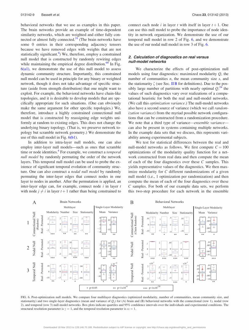
FIG. 6. Post-optimization null models. We compare four multilayer diagnostics (optimized modularity, number of communities, mean community size, and

stationarity) and two single-layer diagnostics (mean and variance of Qs) for (A) brain and (B) behavioral networks with the connectional (row 1), nodal (row

2), and temporal (row 3) null-model networks. Box plots indicate quartiles and 95% confidence intervals over the individuals and experimental conditions. The

structural resolution parameter is c ¼ 1, and the temporal resolution parameter is x ¼ 1.



(60 brain networks and 66 behavioral networks; see “Sec.

II”). We then investigate whether the set of representative

diagnostics for the networks constructed from real data are

different from those of appropriate ensembles of null-model

networks. To address this issue, we subtract the diagnostic

value for the null model from that of the real network for

each subject and experimental session. We then use one-

sample t-tests to determine whether the resulting distribution

differs significantly from 0. We show our results in Fig. 6.

Results depend on all three factors (the data set, the null

model, and the diagnostic), but there do seem to be some gen-

eral patterns. For example, the real networks exhibit the most

consistent differences from the nodal null model for all diag-

nostics and both data sets (see row 2 of Fig. 6). For both data

sets, the variance of single-layer modularity in the real net-

works is consistently greater than those for all three null mod-

els, irrespective of the mean (see the final two columns of

Figs. 6(a) and 6(b)); this is a potential indication of the statis-

tical significance of the temporal evolution. However,

although optimized modularity is higher in the real network

for both data sets, the number of communities is higher in the

set of brain networks and lower in the set of behavioral net-

works. Similarly, in comparison to the connectional null

model, higher modularity is associated with a smaller mean

community size in the brain networks but a larger mean size

in the behavioral networks (see row 1 of Fig. 6). These results

demonstrate that the three post-optimization null models pro-

vide different information about the network structure of the

two systems and thereby underscores the critical need for fur-

ther investigations of null-model construction.

C. Structural and temporal resolution parameters

When optimizing multilayer modularity, we must choose

(or otherwise derive) values for the structural resolution

parameter c and the temporal resolution parameter x. By

varying c, one can tune the size of communities within a

given layer: large values of c yield more communities, and

small values yield fewer communities. A systematic method

for how to determine values of xjlr has not yet been discussed

in the literature. In principle, one could choose different xjlr

values for different nodes, but we focus on the simplest sce-

nario in which the value of xjlr � x is identical for all nodes

j and all contiguous pairs of layers l and r (and is otherwise

0). In this framework, the temporal resolution parameter xprovides a means of tuning the number of communities dis-

covered across layers: high values of x yield fewer commun-

ities, and low values yield more communities. It is beneficial

to study a range of parameter values to examine the breadth

of structural (i.e., intra-layer24,25,71) and temporal (i.e., inter-

layer) resolutions of community structure, and some papers

have begun to make progress in this direction.3,4,13,31,72

To characterize community structure as a function of

resolution-parameter values (and hence of system scales), we

quantify the quality of partitions using the mean value of

optimized Q. To do this, we examine the constitution of the

partitions using the mean similarity over C optimizations,

and we compute partition similarities using the z-score of the

Rand coefficient.73 For comparing two partitions a and b, we

calculate the Rand z-score in terms of the network’s total

number of pairs of nodes M, the number of pairs Ma that are

in the same community in partition a, the number of pairs

Mb that are in the same community in partition b, and the

number of pairs wab that are assigned to the same community

both in partition a and in partition b. The z-score of the Rand

coefficient comparing these two partitions is

zab ¼1

rwab

wab �MaMb

M

� �; (14)

where rwab is the standard deviation of wab (as in Ref. 73).

Let the mean partition similarity z denote the mean value of

zab over all possible partition pairs for a 6¼ b.

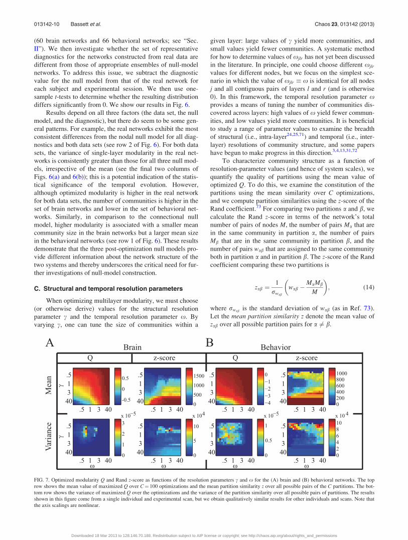
FIG. 7. Optimized modularity Q and Rand z-score as functions of the resolution parameters c and x for the (A) brain and (B) behavioral networks. The top

row shows the mean value of maximized Q over C¼ 100 optimizations and the mean partition similarity z over all possible pairs of the C partitions. The bot-

tom row shows the variance of maximized Q over the optimizations and the variance of the partition similarity over all possible pairs of partitions. The results

shown in this figure come from a single individual and experimental scan, but we obtain qualitatively similar results for other individuals and scans. Note that

the axis scalings are nonlinear.



In Fig. 7, we show both z and optimized Q as a function

of c and x in both brain and behavioral networks. The highest

modularity values occur for low c and high x. The mean par-

tition similarity is high for large c in the brain networks, and

it is high for both small and large c in the behavioral net-

works. Interestingly, in both systems, the partition similarity

when c ¼ x ¼ 1 is lower than it is elsewhere in the ðc;xÞ pa-

rameter plane, so the variability in partitions tends to be large

at this point. Indeed, as shown in the second row of Fig. 7,

modularity exhibits significant variability for c ¼ x ¼ 1

compared to other resolution-parameter values.

It is useful to be able to determine the ranges of c and xthat produce community structure that is significantly differ-

ent from a particular null model. One can thereby use null

models to probe resolution-parameter values at which a net-

work displays interesting structures. This could be especially

useful in systems for which one wishes to identify length

scales (such as a characteristic mean community size) or time

scales4,35,74,75 directly from data.

In Fig. 8, we show examples of how the difference

between diagnostic values for real and null-model networks

varies as a function of c and x. As illustrated in panels (A)

FIG. 8. Differences, as a function of c and x, between the real networks and the (A,B) nodal and (C,D) temporal null models for maximized modularity Q and

partition similarity z for the (A,C) brain and (B,D) behavioral networks. The first row in each panel gives the difference in the mean values of the diagnostic

variables between the real and null-model networks. Panels (A,B) show the results for Q� Qn and z� zn, and panels (C,D) show the results for Q� Qt and

z� zt. The quantities Q and z again denote the modularity and partition similarity of the real network, Qn and zn denote the modularity and partition similarity

of the nodal null-model network, and Qt and zt denote the modularity and partition similarity of the temporal null-model network. The second row in each

panel gives the difference between the optimization variance of the real network and the randomization variance of the null-model network for the same diag-

nostic variable pairs. The third row in each panel gives the difference in the optimization variance of the real network and the optimization variance of the

null-model network for the same diagnostic variable pairs. We show results for a single individual and scan in the experiment, but results are qualitatively sim-

ilar for other individuals and scans. Note that the axis scalings are nonlinear.



and (B), the brain and behavioral networks both exhibit a dis-

tinctly higher mean optimized modularity than the associated

nodal null-model network for c � x � 1. Interestingly, this

roundly peaked difference in Q is not evident in comparisons

of the real networks to temporal null-model networks (see

Figs. 8(c) and 8(d)), so resolution-parameter values (and

hence system scales) of potential interest might be more iden-

tifiable by comparison to nodal than to temporal null models

in these examples. It is possible, however, that defining tem-

poral layers over a longer or shorter duration would yield

identifiable peaks in the difference in Q.

The differences in the Rand z-score landscapes are more

difficult to interpret, as the values of mean partition similarity

z are much larger in the real networks for some resolution-

parameter values (positive differences; red) but are much

larger in the null-model networks for other resolution-

parameter values (negative differences; blue). The clearest sit-

uation occurs when comparing the brain’s real and temporal

null-model networks (see Fig. 8(c)), as the network built from

real data exhibits a much larger value of z (and hence much

more consistent optimization solutions) than the temporal

null-model networks for high values of c (i.e., when there are

many communities) and low x (i.e., when there is weak tem-

poral coupling). These results are consistent with the fact that

weak temporal coupling in a multilayer network facilitates

greater temporal variability in network partitions across time.

Such variability appears to be significantly different than the

noise induced by scrambling time layers. These results suggest

potential resolution values of interest for the brain system, as

partitions are very consistent across many optimizations. For

example, it would be interesting to investigate community

structure in these networks for high c (e.g., c � 40) and low x(e.g., x � 0:1). At these resolution values, one can identify

smaller communities with greater temporal variability than the

communities identified for the case of c ¼ x ¼ 1.4

The optimization and randomization variances appear to

be similar in the brain and behavioral networks (see rows 2–3

in every panel of Fig. 8) not only in terms of their mean values

but also in terms of their distribution in the part of the ðc;xÞparameter plane that we examined. In particular, the variance

in Q is larger in the real networks precisely where the mean is

also larger, so mean and variance are likely either dependent

on one another or on some common source. Importantly, such

dependence influences the ability to draw statistical conclu-

sions because it is possible that the points in the ðc;xÞ plane

with the largest differences in mean are not necessarily the

points with the most significant differences in mean.

We also find that the dependencies of the diagnostics on

c and x are consistent across subjects and scans, suggesting

that our results are ensemble-specific rather than individual-

specific.

D. Examination of data generated from a dynamicalsystem

Real-world data are often clouded by unknown or math-

ematically undefinable sources of variance, so it is also im-

portant to examine data sets generated from dynamical

systems (or other models). Because we are concerned with

time-dependent networks, we consider an example consist-

ing of time-dependent data generated by a well-known dy-

namical system.

We construct a network of Kuramoto oscillators, in

which the phase hiðtÞ of the ith oscillator evolves in time

according to

dhi

dt¼ xi þ

Xj

jAij sinðhj � hiÞ ; i 2 1;…;Nf g ; (15)

where xi is the natural frequency of oscillator i, the matrix A

gives the binary coupling between each pair of oscillators,

and j is a positive real constant that indicates the strength of

the coupling. We draw the frequencies xi from a Gaussian

distribution with mean 0 and standard deviation 1. In our

simulations, we use a time step of s ¼ 0:1, a constant of

j ¼ 0:2, and a network size of N¼ 128.

Kuramoto oscillators have been studied in the context of

various network topologies and geometries51–53,76–78 and

from both the component and ensemble perspectives.79 We

are interested in networks with dynamic community struc-

ture. Following Refs. 77 and 80, we impose a well-defined

community structure in which each community is composed

of 16 nodes. In each time step, each node has 13 connections

with nodes in its own community and 1 connection with

nodes outside of its community (see Fig. 9(a)).

To quantify the temporal evolution of synchronization

patterns, we define a set of temporal networks given by the

time-dependent correlation between pairs of oscillators

/ijðtÞ ¼ hjcos½hiðtÞ � hjðtÞ�ji ; (16)

where the angular brackets indicate an average over 20 simu-

lations. As time evolves from time step t¼ 0 to t¼ 100,

oscillators tend to synchronize with other oscillators in their

same community more quickly than with oscillators in other

communities (see Fig. 9(b)).

To examine the performance of our multilayer

community-detection techniques in this example, we compute

Aijl ¼ Aijt ¼ /i;jðtÞ and using the multilayer extension of the

Newman-Girvan null model Pijl given in Eq. (8). We sepa-

rately optimize Q for two temporal regimes: (1) regime I

(with t 2 f1;…; 50g), for which the synchronization within

communities increases rapidly; and (2) regime II (with

t 2 f51;…; 100g), for which the within-community synchro-

nization level is roughly constant but the global synchroniza-

tion still increases gradually. We set x ¼ 1 and probe the

effects of the structural resolution parameter c in regime II. In

Figs. 9(c) and 9(d), we illustrate that one can identify the

value of c that best uncovers the underlying hard-wired con-

nectivity using troughs in the optimization variance of several

diagnostics (e.g., maximized modularity, number of com-

munities, and mean partition similarity).

We probe the community structure in regime I using the

value of c that best uncovered the underlying hard-wired con-

nectivity in regime II. We observe temporal changes of com-

munity structure at early time points, as evidenced by the

large number of communities for t 2 f1;…; 5g (see Figs. 9(e)

and 9(f)). Importantly, the temporal dependence of community



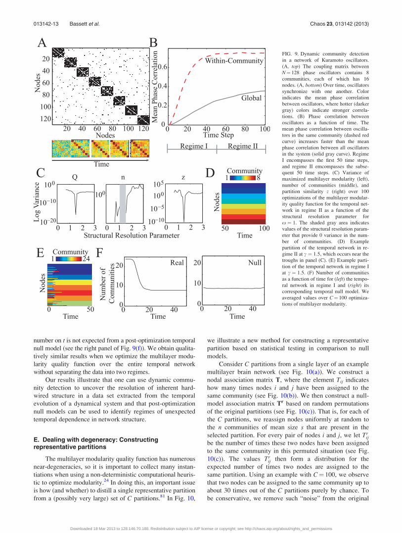
number on t is not expected from a post-optimization temporal

null model (see the right panel of Fig. 9(f)). We obtain qualita-

tively similar results when we optimize the multilayer modu-

larity quality function over the entire temporal network

without separating the data into two regimes.

Our results illustrate that one can use dynamic commu-

nity detection to uncover the resolution of inherent hard-

wired structure in a data set extracted from the temporal

evolution of a dynamical system and that post-optimization

null models can be used to identify regimes of unexpected

temporal dependence in network structure.

E. Dealing with degeneracy: Constructingrepresentative partitions

The multilayer modularity quality function has numerous

near-degeneracies, so it is important to collect many instan-

tiations when using a non-deterministic computational heuris-

tic to optimize modularity.24 In doing this, an important issue

is how (and whether) to distill a single representative partition

from a (possibly very large) set of C partitions.81 In Fig. 10,

we illustrate a new method for constructing a representative

partition based on statistical testing in comparison to null

models.

Consider C partitions from a single layer of an example

multilayer brain network (see Fig. 10(a)). We construct a

nodal association matrix T, where the element Tij indicates

how many times nodes i and j have been assigned to the

same community (see Fig. 10(b)). We then construct a null-

model association matrix Tr based on random permutations

of the original partitions (see Fig. 10(c)). That is, for each of

the C partitions, we reassign nodes uniformly at random to

the n communities of mean size s that are present in the

selected partition. For every pair of nodes i and j, we let Trij

be the number of times these two nodes have been assigned

to the same community in this permuted situation (see Fig.

10(c)). The values Trij then form a distribution for the

expected number of times two nodes are assigned to the

same partition. Using an example with C¼ 100, we observe

that two nodes can be assigned to the same community up to

about 30 times out of the C partitions purely by chance. To

be conservative, we remove such “noise” from the original

FIG. 9. Dynamic community detection

in a network of Kuramoto oscillators.

(A, top) The coupling matrix between

N¼ 128 phase oscillators contains 8

communities, each of which has 16

nodes. (A, bottom) Over time, oscillators

synchronize with one another. Color

indicates the mean phase correlation

between oscillators, where hotter (darker

gray) colors indicate stronger correla-

tions. (B) Phase correlation between

oscillators as a function of time. The

mean phase correlation between oscilla-

tors in the same community (dashed red

curve) increases faster than the mean

phase correlation between all oscillators

in the system (solid gray curve). Regime

I encompasses the first 50 time steps,

and regime II emcompasses the subse-

quent 50 time steps. (C) Variance of

maximized multilayer modularity (left),

number of communities (middle), and

partition similarity z (right) over 100

optimizations of the multilayer modular-

ity quality function for the temporal net-

work in regime II as a function of the

structural resolution parameter for

x ¼ 1. The shaded gray area indicates

values of the structural resolution param-

eter that provide 0 variance in the num-

ber of communities. (D) Example

partition of the temporal network in re-

gime II at c ¼ 1:5, which occurs near the

troughs in panel (C). (E) Example parti-

tion of the temporal network in regime I

at c ¼ 1:5. (F) Number of communities

as a function of time for (left) the tempo-

ral network in regime I and (right) its

corresponding temporal null model. We

averaged values over C¼ 100 optimiza-

tions of multilayer modularity.



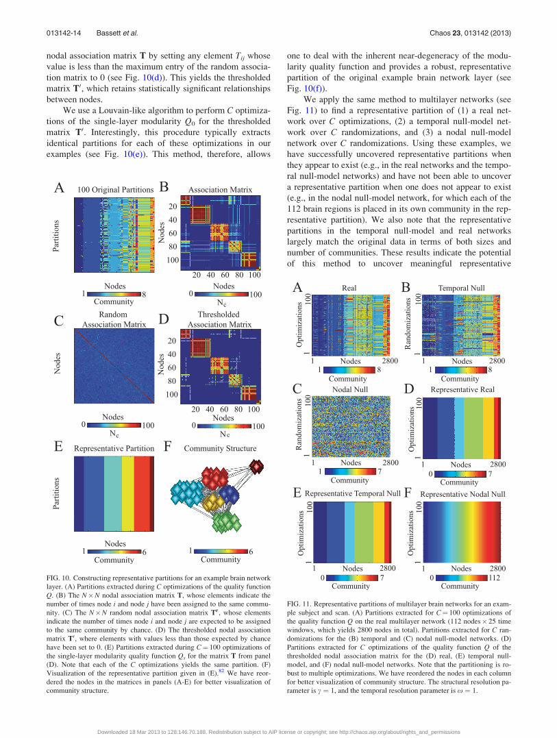
nodal association matrix T by setting any element Tij whose

value is less than the maximum entry of the random associa-

tion matrix to 0 (see Fig. 10(d)). This yields the thresholded

matrix T0, which retains statistically significant relationships

between nodes.

We use a Louvain-like algorithm to perform C optimiza-

tions of the single-layer modularity Q0 for the thresholded

matrix T0. Interestingly, this procedure typically extracts

identical partitions for each of these optimizations in our

examples (see Fig. 10(e)). This method, therefore, allows

one to deal with the inherent near-degeneracy of the modu-

larity quality function and provides a robust, representative

partition of the original example brain network layer (see

Fig. 10(f)).

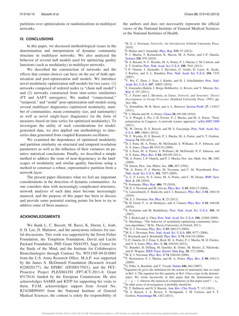
We apply the same method to multilayer networks (see

Fig. 11) to find a representative partition of (1) a real net-

work over C optimizations, (2) a temporal null-model net-

work over C randomizations, and (3) a nodal null-model

network over C randomizations. Using these examples, we

have successfully uncovered representative partitions when

they appear to exist (e.g., in the real networks and the tempo-

ral null-model networks) and have not been able to uncover

a representative partition when one does not appear to exist

(e.g., in the nodal null-model network, for which each of the

112 brain regions is placed in its own community in the rep-

resentative partition). We also note that the representative

partitions in the temporal null-model and real networks

largely match the original data in terms of both sizes and

number of communities. These results indicate the potential

of this method to uncover meaningful representative

FIG. 10. Constructing representative partitions for an example brain network

layer. (A) Partitions extracted during C optimizations of the quality function

Q. (B) The N�N nodal association matrix T, whose elements indicate the

number of times node i and node j have been assigned to the same commu-

nity. (C) The N�N random nodal association matrix Tr, whose elements

indicate the number of times node i and node j are expected to be assigned

to the same community by chance. (D) The thresholded nodal association

matrix T0, where elements with values less than those expected by chance

have been set to 0. (E) Partitions extracted during C¼ 100 optimizations of

the single-layer modularity quality function Qs for the matrix T from panel

(D). Note that each of the C optimizations yields the same partition. (F)

Visualization of the representative partition given in (E).82 We have reor-

dered the nodes in the matrices in panels (A-E) for better visualization of

community structure.

FIG. 11. Representative partitions of multilayer brain networks for an exam-

ple subject and scan. (A) Partitions extracted for C¼ 100 optimizations of

the quality function Q on the real multilayer network (112 nodes� 25 time

windows, which yields 2800 nodes in total). Partitions extracted for C ran-

domizations for the (B) temporal and (C) nodal null-model networks. (D)

Partitions extracted for C optimizations of the quality function Q of the

thresholded nodal association matrix for the (D) real, (E) temporal null-

model, and (F) nodal null-model networks. Note that the partitioning is ro-

bust to multiple optimizations. We have reordered the nodes in each column

for better visualization of community structure. The structural resolution pa-

rameter is c ¼ 1, and the temporal resolution parameter is x ¼ 1.



partitions over optimizations or randomizations in multilayer

networks.

IV. CONCLUSIONS

In this paper, we discussed methodological issues in the

determination and interpretation of dynamic community

structure in multilayer networks. We also analyzed the

behavior of several null models used for optimizing quality

functions (such as modularity) in multilayer networks.

We described the construction of networks and the

effects that certain choices can have on the use of both opti-

mization and post-optimization null models. We introduce

novel modularity-optimization null models for two cases: (1)

networks composed of ordered nodes (a “chain null model”)

and (2) networks constructed from time-series similarities

(FT and AAFT surrogates). We studied “connectional,”

“temporal,” and “nodal” post-optimization null models using

several multilayer diagnostics (optimized modularity, num-

ber of communities, mean community size, and stationarity)

as well as novel single-layer diagnostics (in the form of

measures based on time series for optimized modularity). To

investigate the utility of such considerations for model-

generated data, we also applied our methodology to time-

series data generated from coupled Kuramoto oscillators.

We examined the dependence of optimized modularity

and partition similarity on structural and temporal resolution

parameters as well as the influence of their variances on pu-

tative statistical conclusions. Finally, we described a simple

method to address the issue of near-degeneracy in the land-

scapes of modularity and similar quality functions using a

method to construct a robust, representative partition from a

network layer.

The present paper illustrates what we feel are important

considerations in the detection of dynamic communities. As

one considers data with increasingly complicated structures,

network analyses of such data must become increasingly

nuanced, and the purpose of this paper has been to discuss

and provide some potential starting points for how to try to

address some of these nuances.

ACKNOWLEDGMENTS

We thank L. C. Bassett, M. Bazzi, K. Doron, L. Jeub,

S. H. Lee, D. Malinow, and the anonymous referees for use-

ful discussions. This work was supported by the Errett Fisher

Foundation, the Templeton Foundation, David and Lucile

Packard Foundation, PHS Grant NS44393, Sage Center for

the Study of the Mind, and the Institute for Collaborative

Biotechnologies through Contract No. W911NF-09-D-0001

from the U.S. Army Research Office. M.A.P. was supported

by the James S. McDonnell Foundation (Research Award

#220020177), the EPSRC (EP/J001759/1), and the FET-

Proactive Project PLEXMATH (FP7-ICT-2011-8; Grant

#317614) funded by the European Commission. He also

acknowledges SAMSI and KITP for supporting his visits to

them. P.J.M. acknowledges support from Award No.

R21GM099493 from the National Institute of General

Medical Sciences; the content is solely the responsibility of

the authors and does not necessarily represent the official

views of the National Institute of General Medical Sciences

or the National Institutes of Health.

1M. E. J. Newman, Networks: An Introduction (Oxford University Press,

2010).2P. Holme and J. Saram€aki, Phys. Rep. 519, 97 (2012).3P. J. Mucha, T. Richardson, K. Macon, M. A. Porter, and J.-P. Onnela,

Science 328, 876 (2010).4D. S. Bassett, N. F. Wymbs, M. A. Porter, P. J. Mucha, J. M. Carlson, and

S. T. Grafton, Proc. Natl. Acad. Sci. U.S.A. 108, 7641 (2011).5J.-P. Onnela, J. Saram€aki, J. Hyv€onen, G. Szab�o, D. Lazer, K. Kaski,

J. Kert�esz, and A. L. Barab�asi, Proc. Natl. Acad. Sci. U.S.A. 104, 7332

(2007).6Y. Wu, C. Zhou, J. Xiao, J. Kurths, and H. J. Schellnhuber, Proc. Natl.

Acad. Sci. U.S.A. 107, 18803 (2010).7S. Gonza�alez-Bail�on, J. Borge-Holthoefer, A. Rivero, and Y. Moreno, Sci.

Rep. 1, 197 (2011).8T. J. Fararo and J. Skvoretz, in Status, Network, and Structure: TheoryDevelopment in Group Processes (Stanford University Press, 1997), pp.

362–386.9A. Stomakhin, M. B. Short, and A. L. Bertozzi, Inverse Probl. 27, 115013

(2011).10P. J. Mucha and M. A. Porter, Chaos 20, 041108 (2010).11A. S. Waugh, L. Pei, J. H. Fowler, P. J. Mucha, and M. A. Porter, “Party

polarization in Congress: A network science approach,” arXiv:0907.3509

(2011).12K. W. Doron, D. S. Bassett, and M. S. Gazzaniga, Proc. Natl. Acad. Sci.

U.S.A. 109, 18661 (2012).13N. F. Wymbs, D. S. Bassett, P. J. Mucha, M. A. Porter, and S. T. Grafton,

Neuron 74, 936 (2012).14D. J. Fenn, M. A. Porter, M. McDonald, S. Williams, N. F. Johnson, and

N. S. Jones, Chaos 19, 033119 (2009).15D. J. Fenn, M. A. Porter, S. Williams, M. McDonald, N. F. Johnson, and

N. S. Jones, Phys. Rev. E 84, 026109 (2011).16M. A. Porter, J.-P. Onnela, and P. J. Mucha, Not. Am. Math. Soc. 56, 1082

(2009).17H. Simon, Proc. Am. Philos. Soc. 106, 467 (1962).18M. A. Porter, P. J. Mucha, M. Newman, and C. M. Warmbrand, Proc.

Natl. Acad. Sci. U.S.A. 102, 7057 (2005).19A. C. F. Lewis, N. S. Jones, M. A. Porter, and C. M. Deane, BMC Syst.

Biol. 4, 100 (2010).20S. Fortunato, Phys. Rep. 486, 75 (2010).21M. E. J. Newman and M. Girvan, Phys. Rev. E 69, 026113 (2004).22A. Lancichinetti, F. Radicchi, and J. J. Ramasco, Phys. Rev. E 81, 046110

(2010).23M. E. J. Newman, Nat. Phys. 8, 25 (2012).24B. H. Good, Y. A. de Montjoye, and A. Clauset, Phys. Rev. E 81, 046106

(2010).25S. Fortunato and M. Barth�elemy, Proc. Natl. Acad. Sci. U.S.A. 104, 36

(2007).26P. J. Bickel and A. Chen, Proc. Natl. Acad. Sci. U.S.A. 106, 21068 (2009).27S. Hutchings, “The behavior of modularity-optimizing community detec-

tion algorithms,” M.Sc. Thesis (University of Oxford, 2011).28M. E. J. Newman, Phys. Rev. E 69, 066133 (2004).29M. E. J. Newman, Proc. Natl. Acad. Sci. U.S.A. 103, 8577 (2006).30J. Reichardt and S. Bornholdt, Phys. Rev. E 74, 016110 (2006).31J.-P. Onnela, D. J. Fenn, S. Reid, M. A. Porter, P. J. Mucha, M. D. Fricker,

and N. S. Jones, Phys. Rev. E. 86, 036104 (2012).32U. Brandes, D. Delling, M. Gaertler, R. G€orke, M. Hoefer, Z. Nikoloski,

and D. Wagner, IEEE Trans. Knowl. Data Eng. 20, 172 (2008).33M. E. J. Newman, Phys. Rev. E 74, 036104 (2006).34T. Richardson, P. J. Mucha, and M. A. Porter, Phys. Rev. E 80, 036111

(2009).35G. Palla, A. Barab�asi, and T. Vicsek, Nature 446, 664 (2007).36Equation (4) gives the definition for the notion of stationarity that we used

in Ref. 4. The equation for this quantity in Ref. 4 has a typo in the denomi-

nator. We wrote incorrectly in that paper that the denominator was

t0 � t0 � 1, whereas the numerical computations in that paper used t0 � t0.37In other areas of investigation, it probably should be.38E. T. Bullmore and D. S. Bassett, Ann. Rev. Clin. Psych. 7, 113 (2011).39D. S. Bassett, J. A. Brown, V. Deshpande, J. M. Carlson, and S. T.

Grafton, Neuroimage 54, 1262 (2011).



http://dx.doi.org/10.1016/j.physrep.2012.03.001

http://dx.doi.org/10.1126/science.1184819

http://dx.doi.org/10.1073/pnas.1018985108




http://dx.doi.org/10.1038/srep00197


http://dx.doi.org/10.1088/0266-5611/27/11/115013

http://dx.doi.org/10.1063/1.3518696

http://arxiv.org/abs/0907.3509



http://dx.doi.org/10.1016/j.neuron.2012.03.038

http://dx.doi.org/10.1063/1.3184538

http://dx.doi.org/10.1103/PhysRevE.84.026109



http://dx.doi.org/10.1186/1752-0509-4-100

http://dx.doi.org/10.1186/1752-0509-4-100




http://dx.doi.org/10.1038/nphys2162








http://dx.doi.org/10.1109/TKDE.2007.190689



http://dx.doi.org/10.1038/nature05670

http://dx.doi.org/10.1146/annurev-clinpsy-040510-143934

http://dx.doi.org/10.1016/j.neuroimage.2010.09.006

40A. Zalesky, A. Fornito, I. H. Harding, L. Cocchi, M. Yucel, C. Pantelis,

and E. T. Bullmore, Neuroimage 50, 970 (2010).41J. Wang, L. Wang, Y. Zang, H. Yang, H. Tang, Q. Gong, Z. Chen, C. Zhu,

and Y. He, Hum. Brain Mapp 30, 1511 (2009).42S. Bialonski, M. T. Horstmann, and K. Lehnertz, Chaos 20, 013134

(2010).43A. A. Ioannides, Curr. Opin. Neurobiol. 17, 161 (2007).44C. T. Butts, Science 325, 414 (2009).45G. Kossinets, Soc. Networks 28, 247 (2006).46A. Clauset, C. Moore, and M. E. J. Newman, Nature 453, 98 (2008).47R. Guimer�a and M. Sales-Pardo, Proc. Natl. Acad. Sci. U.S.A. 106, 22073

(2009).48M. Kim and J. Leskovec, SIAM International Conference on Data Mining

(2011).49O. Sporns, Networks of the Brain (MIT, 2010).50E. Bullmore and O. Sporns, Nat. Rev. Neurosci. 10, 186 (2009).51D. M. Abrams and S. H. Strogatz, Phys. Rev. Lett. 93, 174102 (2004).52Y. Kuramoto and D. Battogtokh, Nonlinear Phenom. Complex Syst. 5,

380 (2002).53S. I. Shima and Y. Kuramoto, Phys. Rev. E 69, 036213 (2004).54K. J. Friston, Hum. Brain Mapp 2, 56 (1994).55Y. Benjamini and Y. Yekutieli, Ann. Stat. 29, 1165 (2001).56E. Bullmore and O. Sporns, Nat. Rev. Neurosci. 13, 336 (2012).57V. D. Blondel, J. L. Guillaume, R. Lambiotte, and E. Lefebvre, J. Stat.

Mech. 10, P10008 (2008).58I. S. Jutla, L. G. S. Jeub, and P. J. Mucha, “A generalized Louvain method

for community detection implemented in MATLAB,” (2011–2012); http://

netwiki.amath.unc.edu/GenLouvain.59A discrete time series can be represented as a vector. A continuous time

series would first need to be discretized.60D. Prichard and J. Theiler, Phys. Rev. Lett. 73, 951 (1994).61The code used for this computation actually operates on ½0; 2p�. However,

this should be an equivalent mathematical estimate to the same computa-

tion on ½0; 2pÞ, which is the same except for a set of measure zero.62H. Nakatani, I. Khalilov, P. Gong, and C. van Leeuwen, Phys. Lett. A 319,

167 (2003).63A. Zalesky, A. Fornito, and E. Bullmore, Neuroimage 60, 2096 (2012).

64J. Theiler, S. Eubank, A. Longtin, B. Galdrikian, and J. D. Farmer, Physica

D 58, 77 (1992).65It is also important to note that the AAFT method can allow nonlinear corre-

lations to remain in the surrogate data. Therefore, the development of alterna-

tive surrogate data generation methods might be necessary (Refs. 83 and 84).66In the descriptions below, we use terms like “random” rewiring to refer to

a process that we are applying uniformly at random aside from specified

constraints.67D. Garlaschelli, New J. Phys. 11, 073005 (2009).68S. Maslov and K. Sneppen, Science 296, 910 (2002).69G. Ansmann and K. Lehnertz, Phys. Rev. E 84, 026103 (2011).70S. Bialonski, M. Wendler, and K. Lehnertz, PLoS ONE 6, e22826

(2011).71V. A. Traag, P. Van Dooren, and Y. Nesterov, Phys. Rev. E 84, 016114

(2011).72K. T. Macon, P. J. Mucha, and M. A. Porter, Physica A 391, 343 (2012).73A. L. Traud, E. D. Kelsic, P. J. Mucha, and M. A. Porter, SIAM Rev. 53,

526 (2011).74D. S. Bassett, E. T. Owens, K. E. Daniels, and M. A. Porter, Phys. Rev. E

86, 041306 (2012).75X. Lou and J. A. Suykens, Chaos 21, 043116 (2011).76A. Arenas, A. D�ıaz-Guilera, J. Kurths, Y. Moreno, and C. Zhou, Phys.

Rep. 469, 93 (2008).77A. Arenas, A. D�ıaz-Guilera, and C. J. P�erez-Vicente, Phys. Rev. Lett. 96,

114102 (2006).78J. Stout, M. Whiteway, E. Ott, M. Girvan, and T. M. Antonsen, Chaos 21,

025109 (2011).79G. Barlev, T. M. Antonsen, and E. Ott, Chaos 21, 025103 (2011).80A. Arenas, A. D�ıaz-Guilera, and C. J. P�erez-Vicente, Physica D 224, 27

(2006).81A. Lancichinetti and S. Fortunato, Sci. Rep. 2, 336 (2012).82A. L. Traud, C. Frost, P. J. Mucha, and M. A. Porter, Chaos 19, 041104

(2009).83C. R€ath, M. Gliozzi, I. E. Papadakis, and W. Brinkmann, Phys. Rev. Lett.

109, 144101 (2012).84G. Rossmanith, H. Modest, C. R€ath, A. J. Banday, K. M. Gorski, and

G. Morfill, Phys. Rev. D 86, 083005 (2012).




http://dx.doi.org/10.1002/hbm.20623

http://dx.doi.org/10.1063/1.3360561

http://dx.doi.org/10.1016/j.conb.2007.03.008


http://dx.doi.org/10.1016/j.socnet.2005.07.002

http://dx.doi.org/10.1038/nature06830


http://dx.doi.org/10.1038/nrn2575

http://dx.doi.org/10.1103/PhysRevLett.93.174102


http://dx.doi.org/10.1002/hbm.460020107

http://dx.doi.org/10.1214/aos/1013699998

http://dx.doi.org/10.1038/nrn3214

http://netwiki.amath.unc.edu/GenLouvain

http://netwiki.amath.unc.edu/GenLouvain


http://dx.doi.org/10.1016/j.physleta.2003.09.082


http://dx.doi.org/10.1016/0167-2789(92)90102-S

http://dx.doi.org/10.1016/0167-2789(92)90102-S

http://dx.doi.org/10.1088/1367-2630/11/7/073005



http://dx.doi.org/10.1371/journal.pone.0022826


http://dx.doi.org/10.1016/j.physa.2011.06.030

http://dx.doi.org/10.1137/080734315


http://dx.doi.org/10.1063/1.3655371




http://dx.doi.org/10.1063/1.3581168

http://dx.doi.org/10.1063/1.3596711

http://dx.doi.org/10.1016/j.physd.2006.09.029


http://dx.doi.org/10.1063/1.3194108


http://dx.doi.org/10.1103/PhysRevD.86.083005

Robust detection of dynamic community structure in networksmason/papers/dani-chaos-final.pdf ·...

Documents

Transcript of Robust detection of dynamic community structure in networksmason/papers/dani-chaos-final.pdf ·...