ROBUST CONVEX OPTIMIZATION - Atlanta, GAnemirovs/MOR_RCO_1998.pdf · We study convex optimization...

/ 3907 no28 Mp 769 Monday Dec 21 01:08 PM INF–MOR no28

769

0364-765X/98/2304/0769/$05.00Copyright q 1998, Institute for Operations Research and the Management Sciences

MATHEMATICS OF OPERATIONS RESEARCHVol. 23, No. 4, November 1998Printed in U.S.A.

ROBUST CONVEX OPTIMIZATION

A. BEN-TAL AND A. NEMIROVSKI

We study convex optimization problems for which the data is not specified exactly and it isonly known to belong to a given uncertainty set U, yet the constraints must hold for all possiblevalues of the data from U. The ensuing optimization problem is called robust optimization. In thispaper we lay the foundation of robust convex optimization. In the main part of the paper we showthat if U is an ellipsoidal uncertainty set, then for some of the most important generic convexoptimization problems (linear programming, quadratically constrained programming, semidefiniteprogramming and others) the corresponding robust convex program is either exactly, or approx-imately, a tractable problem which lends itself to efficient algorithms such as polynomial timeinterior point methods.

1. Introduction.

Robust counterpart approach to uncertainty. Consider an optimization problem ofthe form

(p ) min f ( x , z)znx√R

ms.t. F(x , z) √ K , R ,(1)

wherej z √ RM is the data element of the problem;j x √ R n is the decision vector;j the dimensions n , m , M , the mappings f (·, ·) , F(·, ·) and the convex cone K are

structural elements of the problem.In this paper we deal with a ‘‘decision environment’’ which is characterized by

(i) A crude knowledge of the data: it may be partly or fully ‘‘uncertain,’’ and all thatis known about the data vector z is that it belongs to a given uncertainty set U , RM

( ii ) The constraints F(x , z) √ K must be satisfied, whatever the actual realization ofz √ U is.

In view of (i) and (ii) we call a vector x feasible solution to the uncertain optimizationproblem (P) Å {(pz)}z√U , if x satisfies all possible realizations of the constraints:

F(x , z) √ K ∀z √ U.(2)

Note that this is the same notion of feasibility as in Robust Control (see, e.g., Zhou, Doyle,and Glover 1995).

We can define in the same manner the notion of an optimal solution to the uncertainoptimization problem (P) : such a solution must give the best possible guaranteed value

Received January 13, 1997; revised: November 13, 1997; April 24, 1998.AMS 1991 subject classification. Primary: 90C05, 90C25, 90C30.OR/MS Index 1978 subject classification. Primary: Programming/Convex.Key words. Convex optimization, data uncertainty, robustness, linear programming, quadratic programming,semidefinite programming, geometric programming.

770 BEN-TAL AND NEMIROVSKI


sup f ( x , z)z√U

of the original objective under constraints (2) , i.e., it should be an optimal solution to thefollowing ‘‘certain’’ optimization problem

(P*) min sup f ( x , z) : F(x , z) √ K ∀z √ U .H Jz√U

From now on we call feasible/optimal solutions to (P*) robust feasible /optimal solutionsto the uncertain optimization problem (P) , and the optimal value in (P*) is called therobust optimal value of uncertain problem (P) ; the problem (P*) itself will be called therobust counterpart of (P) .

Motivation. The ‘‘decision environment’’ we deal with is typical for many applica-tions. The reasons for a crude knowledge of the data may be:

j z is unknown at the time the values of x should be determined and will be realizedin the future, e.g., x is a vector of production variables and z comprises future demands,market prices, etc., or: x represents the cross-sections of bars in a truss construction likea bridge, and z represents locations and magnitudes of future loads the bridge will haveto carry, etc.

j z is realizable at the time x is determined, but it cannot be measured/estimated/computed exactly, e.g., material properties like Young’s modulus, pressures and temper-atures in remote places, . . . .

j Even if the data is certain and an optimal solution x* can be computed exactly, it cannotbe implemented exactly, which is in a sense equivalent to uncertainty in the data. Consider,e.g., a linear programming problem min{cTx : Ax / b ¢ 0, x ¢ 0} of an engineeringorigin, where the components of the decision vector x correspond to ‘‘physical character-istics’’ of the construction to be manufactured (sizes, weights, etc.) . Normally it is knownin advance that what will be actually produced will be not exactly the computed vector x ,but a vector x* with components close (say, within 5% margin) to those of x . This situationis equivalent to the case where there are no inaccuracies in producing x , but there is un-certainty in the constraint matrix A and the objective c —they are known ‘‘up to multipli-cation by a diagonal matrix with diagonal entries varying from 0.95 to 1.05.’’

Situations when the constraints are ‘‘hard,’’ so that ( ii ) is a ‘‘must,’’ are quite commonin reality, especially in engineering applications. Consider, e.g., a typical technologicalprocess in the chemical industry. Such a process consists of several decomposition—recombination stages, the yields of the previous stages being the ‘‘raw materials’’ for thenext one. As a result, the model of the process includes many balance constraints indi-cating that the amount of materials of different types used at a given stage cannot exceedthe amount of these materials produced at the preceding stages. On one hand, the datacoefficients in these constraints are normally inexact—the contents of the input raw ma-terials, the parameters of the devices, etc., typically are ‘‘floating.’’ On the other hand,violation of physical balance constraints can ‘‘kill’’ the process completely and is thereforeinadmissible. Similar situation arises in other engineering applications, where violatingphysical constraints may cause an explosion or a crush of the construction. As a concreteexample of this type, consider the Truss Topology Design (TTD) problem (for moredetails, see Ben-Tal and Nemirovski 1997).

A truss is a construction comprising thin elastic bars linked with each other at nodes—points from a given finite (planar or spatial) set. When subjected to a given load —acollection of external forces acting at some specific nodes—the construction deformates,until the tensions caused by the deformation compensate the external load. The deformated

771ROBUST CONVEX OPTIMIZATION

/ 3907 no28 Mp 771 Monday Dec 21 01:08 PM INF–MOR

FIGURE 1. Cantilever arm: nominal design (left) and robust design (right) .

truss capacitates certain potential energy, and this energy—the compliance—measuresstiffness of the truss (its ability to withstand the load); the less is the compliance, themore rigid is the truss.

In the usual TTD problem we are given the initial nodal set, the external ‘‘nominal’’load and the total volume of the bars. The goal is to allocate this resource to the bars inorder to minimize the compliance of the resulting truss.

Fig. 1 (a ) shows a cantilever arm which withstands optimally the nominal load—the unit force f * acting down at the most right node. The corresponding optimalcompliance is 1.

It turns out that the construction in question is highly unstable: a small force f (10times smaller than f *) depicted by small arrow on Figure 1(a) results in a compliancewhich is more than 3,000 times larger than the nominal one.

In order to improve design’s stability, one may use the robust counterpart methodology.Namely, let us treat the external load as the uncertain data of the associated optimizationproblem. Note that in our example a load is, mathematically, a collection of ten 2D vectorsrepresenting (planar) external forces acting at the ten nonfixed nodes of the cantileverarm; in other words, the data in our problem is a 20-dimensional vector. Assume that theconstruction may be subjected not to the nominal load only, but also to a ‘‘small occasionalload’’ represented by an arbitrary 20-dimensional vector of the Euclidean norm°0.1 (i.e.,of the norm 10 times smaller than the norm of the nominal load). Thus, we allow theuncertain data of our problem to take the nominal value f *, as well as any value fromthe 20-dimensional Euclidean ball B0.1 centered at the origin. In order to get an efficientlysolvable robust counterpart, we extend the resulting data set B0.1 < { f *} to its ‘‘ellipsoidalenvelope’’ U, i.e., the smallest volume 20-dimensional ellipsoid centered at the origin andcontaining f * and B0.1 . This ellipsoid is then taken as our uncertainty set U.

Solving the robust counterpart of the resulting uncertain problem, we get the cantileverarm shown on Fig. 1(b) .

The compliances of the original and the new constructions with respect to the nominalload and their worst-case compliances with respect to the ‘‘occasional loads’’ from B0.1

are as follows:

Design Compliance w.r.t. f* Compliance w.r.t. B0.1

single-load 1 ú3360robust 1.0024 1.003

We see that in this example the robust counterpart approach improvesdramatically the stability of the resulting construction, and that theimprovement is in fact ‘‘costless’’—the robust optimal solution isnearly optimal for the nominal problem as well.



There are of course situations in reality when ‘‘occasional violations’’ of the constraintsare not that crucial, and in these situations the robust counterpart approach may seem tobe too conservative. We believe, however, that even in these situations, the robust opti-mization methodology should be at least tried—it may well happen that ensuring robustfeasibility is ‘‘nearly costless,’’ as it is in the above TTD example and other examplesfrom Ben-Tal and Nemirovski (1997). Problems arising in applications often are highlydegenerate, and as a result possess a quite ‘‘massive’’ set of nearly optimal solutions;ignoring the uncertainty and obtaining the decision by solving the problem with the ‘‘nom-inal’’ data, we normally end up with a point on the boundary of the above set, and sucha point may be a very bad solution to a problem with a slightly perturbed data. In contrastto this, the robust counterpart tries to choose the ‘‘most inner’’ solution from the abovemassive set, and such a solution is normally much more stable w.r.t. data perturbationsthan a boundary one.

Robust counterpart approach vs. traditional ways to treat uncertainty. Uncertaintyis treated in the Operations Research/Engineering literature in several ways. (We referhere to uncertainty in the constraints. For uncertainty in the objective function, there is avast literature in economics, statistics and decision theory.)

j In many cases the uncertainty is simply ignored—at the stage of building the modeland finding an optimal solution uncertain data are replaced with some nominal values,and the only care of uncertainty (if any) is taken by sensitivity analysis . This is a post-optimization tool allowing just to analyze the stability properties of the already generatedsolution. Moreover, this analysis typically can deal only with ‘‘infinitesimal’’ perturba-tions of the nominal data.

j There exist modeling approaches which handle uncertainty directly and from the verybeginning, notably Stochastic Programming. This approach is limited to those cases wherethe uncertainty is of stochastic nature (which is not always the case) and we are able toidentify the underlying probability distributions (which is even more problematic, espe-cially in the large-scale case) . Another essential difference between the SP and the robustcounterpart approaches is that the majority of SP models allow a solution to violate theconstraints affected by uncertainty and thus do not meet the requirement (ii ) .

Another approach to handle uncertainty is ‘‘Robust Mathematical Programming’’(RMP) proposed recently by Mulvey, Vanderbei, and Zenios (1995). Here instead offixed ‘‘nominal’’ data several scenarios are considered, and a candidate solution is allowedto violate the ‘‘scenario realizations’’ of the constraints. These violations are included viapenalty terms in the objective, which allows to take care of the stability of the resultingsolution. The RMP approach again may produce solutions which are not feasible forrealizations of the constraints, even for the scenario ones. When treating the scenariorealizations of the constraints as ‘‘obligatory,’’ the RMP approach, under mild structuralassumptions, becomes a particular case of the robust counterpart scheme, namely, the caseof an uncertainty set given as the convex hull of the scenarios.

Robust counterpart approach: the goal. As we have already mentioned, our approachis motivated by the need to comply with the difficulties imposed by the environmentdescribed in (i) , ( ii ) above. But there is another equally important consideration: forrobust optimization to be an applicable methodology for real life large scale problems, itis essential that

( iii ) The robust counterpart must be ‘‘computationally tractable.’’

At a first glance this requirement looks unachievable, as the robust counterpart (P*)of an uncertain problem (P) is a semi-infinite optimization problem. It is well-known that



semi-infinite programs, even convex, often cannot be efficiently solved numerically, andin particular are not amenable to the use of advanced optimization tools like interior pointmethods. This in practice imposes severe restrictions on the sizes of problems which canbe actually solved. Therefore a goal of primary importance for applications of the robustoptimization approach is converting the robust counterparts of generic convex problemsto ‘‘explicit’’ convex optimization programs, accessible for high-performance optimiza-tion techniques. Possibilities of such a conversion depend not only on the analytical struc-ture of the generic program in question, but also on the geometry of the uncertainty setU. In the case of ‘‘trivial geometry’’ of the uncertainty set, when U is given as a convexhull of a finite set of ‘‘scenarios’’ {z1 , . . . , zN}, the ‘‘conversion problem’’ typicallydoes not arise at all. Indeed, if f ( x , z) and F(x , z) ‘‘depend properly’’ on z , e.g., areaffine in the data (which is the case in many of applications) , the robust counterpart of(P) Å {(pz)}z√U is simply the problem

i imin{t : t ¢ f ( x , z ) , F(x , z ) ¢ 0, i Å 1, . . . , N}.

The analytical structure of this problem is exactly the same as the one of the instances.In our opinion, this simple geometry of the uncertainty set is not that interesting mathe-matically and is rather restricted in its expressive abilities. Indeed, a ‘‘scenario’’ descrip-tion/approximation of typical uncertainty sets (even very simple ones, given by element-wise bounds on the data, or more general standard ‘‘inequality-represented’’ polytopes)requires an unrealistically huge number of scenarios. We believe that more reasonabletypes of uncertainty sets are ellipsoids and intersections of finitely many ellipsoids (thelatter geometry covers also the case of a polytope uncertainty set given by a list of in-equalities—a half-space is a ‘‘very large’’ ellipsoid) . Indeed:

j An ellipsoid is a very convenient entity from the mathematical point of view, it hasa simple parametric representation and can be easily handled numerically.

j In many cases of stochastic uncertain data there are probabilistic arguments allowingto replace stochastic uncertainty by an ellipsoidal deterministic uncertainty. Consider, e.g.,an uncertain Linear Programming (LP) problem with random entries in the constraintmatrix (what follows can be straightforwardly extended to cover the case of randomuncertainty also in the objective and the right-hand side of the constraints) . For a givenx , the left-hand side li (x) Å / bi of the i th constraint in the system ATx / b ¢ 0 isTa xi

a random variable with expectation ei (x) Å / bi , and standard deviation £i (x)T*(a ) xi

Å being the expectation and Vi being the covariance matrix of the random_____√

T *x V x , ai i

vector ai . A ‘‘typical’’ value of the random variable li (x) will therefore be ei (x) {O(£i (x)) , and for a ‘‘light tail’’ distribution of the random data a ‘‘likely’’ lower boundon this random variable is Å ei (x) 0 u£i (x) with ‘‘safety parameter’’ u of order ofPl (x)i

one (cf. the engineers’ ‘‘3s-rule’’ for Gaussian random variables) . This bound leads tothe ‘‘likely reliable’’ version

e (x) 0 u£ (x) ¢ 0i i

of the constraint in question. Now note that the latter constraint is exactly the robustcounterpart

Ta x / b ¢ 0 ∀a √ Ui i i i

of the original uncertain constraint if Ui is specified as the ellipsoid

T 01 2* *U Å {a : (a 0 a ) V (a 0 a ) ° u }.i i i i



j Finally, properly chosen ellipsoids and especially intersections of ellipsoids can beused as reasonable approximations to more complicated uncertainty sets.

As shown later in the paper, in several important cases (linear programming, convexquadratically constrained quadratic programming and some others) the use of ellipsoidaluncertainties leads to ‘‘explicit’’ robust counterparts which can be solved both theoreti-cally and in practice (e.g., by interior-point methods) . The derivation of these ‘‘explicitforms’’ of several generic uncertain optimization problems is our main goal.

Robust counterpart approach: previous work. As already indicated, the approach inquestion is directly related to Robust Control. For Mathematical Programming, this ap-proach seems to be new. The only setting and results of this type known to us are thoseof Singh (1982) and Falk (1976) originating from the 1973 note of A. L. Soyster; thissetting deals with a very specific and in fact the most conservative version of the approach(see discussion in Ben-Tal and Nemirovski 1995a).

The general robust counterpart scheme as outlined below was announced in recent paperof Ben-Tal and Nemirovski (1997) on robust Truss Topology Design. Implementation ofthe scheme in the particular case of uncertain linear programming problems is consideredin Ben-Tal and Nemirovski (1995a). Many of the results of the current paper, and someothers, were announced in Ben-Tal and Nemirovski (1995b). Finally, when working onthe present paper, we became aware of the papers of Oustry, El Ghaoui, and Lebret (1996)and El-Ghaoui and Lebret (1996) which also develop the robust counterpart approach,mainly as applied to uncertain semidefinite programming.

For recent progress in robust settings of discrete optimization problems, see Kouvelisand Yu (1997).

Summary of results. We mainly focus on (a) general development of the robust coun-terpart approach, and (b) applications of the scheme to generic families of nonlinear convexoptimization problems—linear, quadratically constrained quadratic, conic quadratic andsemidefinite ones. As far as (a) is concerned, we start with a formal exposition of the approach(§2.1) and investigate general qualitative (§2.2) and quantitative (§2.3) relations betweensolvability properties of the instances of an uncertain problem and those of its robust coun-terpart. The questions we are interested in are: assume that all instances of an uncertainprogram are solvable. Under what condition is it true that robust counterpart also is solvable?When is there no ‘‘gap’’ between the optimal value of the robust counterpart and the worstof the optimal values of instances? What can be said about the proximity of the robust optimalvalue and the optimal value in a ‘‘nominal’’ instance?

The main part of our efforts is devoted to (b) . We demonstrate thatj The robust counterpart of an uncertain linear programming problem with ellipsoidal or >-

ellipsoidal (intersection of ellipsoids) uncertainty is an explicit conic quadratic program (§3.1).j The robust counterpart of an uncertain convex quadratically constrained quadratic pro-

gramming problem with ellipsoidal uncertainty is an explicit semidefinite program, while ageneral-type >-ellipsoidal uncertainty leads to an NP-hard robust counterpart (§3.2).

j The robust counterpart of an uncertain conic quadratic programming problem with ellip-soidal uncertainty, under some minor restrictions, is an explicit semidefinite program, whilea general-type >-ellipsoidal uncertainty leads to an NP-hard robust counterpart (§3.3).

j In the case of uncertain semidefinite program with a general-type ellipsoidal uncer-tainty set the robust counterpart is NP-hard. We present a generic example of a ‘‘well-structured’’ ellipsoidal uncertainty which results in a tractable robust counterpart (anexplicit semidefinite program). Moreover, we propose a ‘‘tractable’’ approximate robustcounterpart of a general uncertain semidefinite problem (§3.4) .

j We derive an explicit form of the robust counterpart of an affinely parameterizeduncertain problem (e.g., geometric programming problem with uncertain coefficients of



the monomials) (§3.5) and develop a specific saddle point form of the robust counterpartfor these problems (§4).

2. Robust counterparts of uncertain convex programs. In what follows we dealwith parametric convex programs of the type (1) . Technically, it is more convenient to‘‘standardize’’ the objective—to make it linear and data-independent. To this end it suf-fices to add a new variable t to be minimized and to add to the list of original constraintsthe constraint t 0 f ( x , z) ¢ 0. In what follows we assume that such a transformation hasbeen already done, so that the optimization problems in question are of the type

T(p) : min{c x : F(x , z) √ K , x √ X}(3)

wherej x √ R n is the design vector;j c √ R n is a certain ‘‘cost’’ vector;j z √ A , RM is a parameter vector.From now on we make the following assumption (which in particular ensures that (p)

is a convex program whenever z √ A) :ASSUMPTION A.j K , RN is a closed convex cone with a nonempty interior;j X is a closed convex subset in R n with a nonempty interior;j A is a closed convex subset in RM; with a nonempty interior;j F(x , z) : X 1 A r RN is assumed to be continuously differentiable mapping on X

1 A and K-concave in x , i .e .,

∀(x*, x9 √ X, z √ A) ∀(l √ [0, 1]) :

F(lx* / (1 0 l)x9, z) ¢ lF(x*, z) / (1 0 l)F(x9, z) ,K

where ‘‘b ¢K a’’ stands for b 0 a √ K .

2.1. Uncertain convex programs and their robust counterparts. We define an un-certain convex program (P ) as a family of ‘‘instances’’—programs (p) of the type (3)with common structure [n , c , K , F(·, ·)] and the data vector z running through a givenuncertainty set U , A:

T(P) Å {(p) : min{c x : F(x , z) √ K , x √ X}} .(4) z√U

We associate with an uncertain program (P) its robust counterpart—the followingcertain optimization program

T(P*): min{c x : x √ X, F(x , z) √ K ∀z √ U}.

Feasible solutions to (P*) are called robust feasible solutions to (P) , the infimum of thevalues of the objective at robust feasible solutions to (P) is called the robust optimalvalue of (P) , and, finally, an optimal solution to (P*) is called a robust optimal solutionto (P) . Note that (P*) is in fact a semi-infinite optimization problem.

It makes sense (see Propositions 2.1 and 2.2 below) to restrict ourselves to a particularcase of uncertainty—the one which is concave in the data:

DEFINITION 2.1. The uncertain optimization problem (P) has concave uncertainty , ifthe underlying mapping F(x , z) is K-concave in z :



∀(x √ X, z*, z9 √ A) ∀(l √ [0, 1]) :

F(x , lz* / (1 0 l)z9) ¢ lF(x , z*) / (1 0 l)F(x , z9) .K

In some cases we shall speak also about affine uncertainty :

DEFINITION 2.2. The uncertain optimization problem (P) has affine uncertainty , ifthe underlying mapping F(x , z) is affine in z for every x √ X.

As we shall see in a while, a number of important generic convex programs (linear,quadratic, semidefinite, . . .) are indeed affine in the data.

In the case of concave uncertainty we can assume without loss of generality that theuncertainty set U is a closed convex set:

PROPOSITION 2.1. Let (P) be an uncertain convex program with concave uncertainty ,and let (P*) be the uncertain convex program obtained from (P) by replacing the originaluncertainty set U by its closed convex hull . Then the robust counterparts of (P) and (P*)are identical to each other .

PROOF. By assumption A the robust counterpart (P*) clearly remains unchangedwhen we replace U by its closure. Thus, all we need is to verify that in the case of concaveuncertainty the robust counterpart remains unchanged when the uncertainty set is extendedto its convex hull. To this end, in turn, it suffices to verify that if x is robust feasible for(P) and z √ Conv U, then F (x , z) ¢K 0, which is evident: z is a convex combination

lizi of data vectors from U, and due to concavity of F w.r.t. data,k( iÅ1

k

[0 ° ] l F(x , z ) ° F(x , z) . h∑K i i KiÅ1

In view of the above considerations, from now on we make the following

DEFAULT ASSUMPTION. All uncertain problems under consideration satisfy Assump-tion A , and the uncertainty is concave . The uncertainty sets U underlying the problemsare closed and convex .Let us also make the following

DEFAULT NOTATIONAL CONVENTION. Indices of all matrices and vectors are alwayssuperscripts ; denotes the ith row of a matrix A ··· regarded as a row vector .···Ai

2.2. Solvability properties of the robust counterpart. We start with the followingdirect consequence of our Default Assumption:

PROPOSITION 2.2. The feasible set of the robust counterpart (P*) is a closed convexset , so that the robust counterpart of an uncertain convex program is a convex program .If the robust counterpart is feasible , then all instances of the uncertain program arefeasible , and the robust optimal value of the program is greater or equal to the optimalvalues of all the instances .

It is easily seen that in the most general case there could be a substantial ‘‘gap’’ betweenthe solvability properties of the instances of an uncertain program and those of the robustcounterpart of the program, e.g., it may happen that all instances of a given uncertain programare feasible, while the robust counterpart is not, or that the optimal value of the robust coun-terpart is ‘‘essentially worse’’ than the optimal values of all instances (see, e.g., the examplein Ben-Tal and Nemirovski 1995b). There is, however, a rather general case when the above‘‘gap’’ vanishes—this is the case of constraint-wise affine uncertainty.



The notion of a constraint-wise uncertainty relates to the particular case of an uncertainconvex program (P) associated with KÅ where it indeed makes sense to speak aboutmR ,/separate scalar constraints

f (x , z)1

f (x , z) ¢ 0, i Å 1, . . . , m F(x , z) Å ??? .i F S DGf (x , z)m

Note that the robust counterpart of (P) in this case is the program

T(P*): min{c x : x √ X, f (x , z) ¢ 0 ∀i Å 1, . . . , m ∀z √ U}.i

By construction, the robust counterpart remains unchanged if instead thinking of a com-mon data vector z for all constraints we think about a separate data vector for everyconstraint, i.e., instead of the original mapping

f (x , z)1

f (x , z)2 mF(x , z) Å : X 1 A r R???1 2

f (x , z)m

and the original uncertainty set U, we consider the mapping

f (x , z )1 1

f (x , z )2 2 mPF(x , z , . . . , z ) Å : X 1 A 1 ··· 1 A r R1 m ???1 2

f (x , z )m m

and the uncertainty set

PU ÅU 1 ··· 1 U.

m

The constraint-wise uncertainty is exactly the one of the latter type: the i th component ofF depends on x and on the i th portion zi of the data, and the uncertainty set U is a directproduct of closed and convex uncertainty sets Ui in the spaces of zi’s, i Å 1, . . . , m .

THEOREM 2.1. Assume that (P ) is an uncertain problem with constraint-wise affineuncertainty and that the set X is compact . Then the robust counterpart (P*) of the problemis feasible if and only if all instances of the problem are feasible , and in this case therobust optimal value is the supremum of those of the instances .

PROOF. In view of Proposition 2.2 it suffices to prove that if all instances of (P) arefeasible, then (i) (P*) is feasible, and (ii) the optimal value of (P*) is the supremum ofoptimal values of the instances.

To prove (i) , assume, on the contrary, that (P*) is infeasible. Then the family of sets

{X (z ) å {x √ X É f (x , z ) ¢ 0}}i i i i iÅ1, . . . ,m,z√Ui i

has empty intersection. Since all these sets are closed subsets of a compact set X, it follows



that some finite subfamily of the family has empty intersection, so that there exists acollection zi ,j √ Ui , i Å 1, . . . , m , j Å 1, . . . , M such that

> X (z ) Å M,i i ,ji°m, j°M

or, which is the same,

max min f (x , z ) õ 0.i i ,jx√X i°m, j°M

Since all the functions fi (·, zi ,j) are concave and continuous on convex compact set X, itfollows that there exists a convex combination

f ( x) Å l f (x , z )∑ i ,j i i ,j

i°m, j°M

of the functions fi (·, zi ,j) which is strictly negative on X. Let us set

M

l Å l ,∑i i ,j

jÅ1

m01z Å l l z∑i i i ,j i ,j

jÅ1

( in the case of li Å 0, zi is a fixed in advance point from Ui ) . Since fi (x , ·) is affine inzi , we clearly have

M

l f (x , z ) Å l f (x , z ) ,∑i i i i ,j i i ,j

jÅ1

so that

m

l f (x , z ) õ 0 ∀x √ X.(5) ∑ i i i

iÅ1

Since the uncertainty is constraint-wise and the sets Ui are convex, the point z Å (z1 , . . . ,zm) belongs to U; the instance corresponding to the data z is infeasible in view of (5) ,which is a contradiction.

To prove (ii), note that since X is bounded, the supremum (denoted by c*) of optimalvalues of the instances is finite. Now let us add to all instances of the original uncertainproblem (P) the additional ‘‘certain’’ constraint cTx ° c*. Applying (i) to the resultingproblem, we conclude that its robust counterpart is feasible, and hence the optimal value in(P*) is at most (and in view of Proposition 2.2—also at least) c*, as required in (ii). h

2.3. Elementary sensitivity analysis for uncertain programs. In this section we ad-dress the following natural question: let

0 T 0(p ) : min{c x : x √ X, F(x , z ) √ K}(6)

be a ‘‘nominal’’ instance of an uncertain convex program (P) with uncertainty set



0U Å z / V :

T0(P) Å {min{c x : x √ X, F(x , z) √ K}} .z√z /V

Assume that (p 0) is solvable, and let G 0 be the feasible set, be an optimal solution,*x 0

and be the optimal value of this instance.*c 0

Let

T 0(P*): min{c x : x √ X, F(x , z) √ K ∀z √ z / V}

be the robust counterpart of (P) . What can be said about the proximity of the optimalvalue of the nominal instance to that of the robust counterpart (P*)?

We are going to give a partial answer in the case of the mapping F(x , z) being affinein x (and, as always, being K-concave in z) . Even in this particular case the answer clearlyshould impose appropriate restrictions on the nominal instance—in the general case itmay well happen that the robust counterpart is infeasible. We now define a quantity—the feasibility margin of the nominal instance—in terms of which we will express thecloseness of the nominal and the robust optimal values.

DEFINITION 2.3. For x √ G 0 , the feasibility margin lV(x) of x with respect to V is

0 0l (x) Å sup{l ¢ 0 : ∀(d √ V) : [z { ld √ A] & [F(x , z { ld) √ K]}.V

We start with the following

LEMMA 2.1. Let l ú 1, r √ (0, 1) and x √ G0 be such that every point x from the set

0 0G Å (1 0 r)xP / rGr ,xP

satisfies the relation

l (x) ¢ l.(7) V

Let also the mapping F(x , z) be affine in x . Then the optimal value of (P*) satisfiesc*Uthe inequality

2(1 0 r) T* *c* ° c / [c xP 0 c ] ,(8) U 0 0rl / 2 0 r

PROOF. It suffices to prove that the point

y Å xP / vu ,

*u Å x 0 xP ,0

2(1 0 r)v Å 1 0

rl / 2 0 r

r(l / 1)Årl / 2 0 r



is robust feasible (note that the right-hand side in (8) is exactly the value of theobjective at y ) .

Let d √ V. We have the following inclusions:

0F(xP , z 0 ld) √ K ,(9)

0F(xP / ru , z / ld) √ K ,(10)

0F(xP / u , z ) √ K .(11)

Indeed, (9) comes from lV( x) ¢ l, (10) comes from lV( x / ru) ¢ l, and (11) comesfrom F( x / u , z0) Å z0) √ K .*F(x ,0

Note that v ú r due to r √ (0, 1) , l ú 1. Now let

1 0 vm Å ú 0,

2v

1 0 vn Å ú 0.

2(v 0 r)

In view of (9) – (11), for every d √ V we have

0 0 00 ° nF(xP / ru , z / ld) / mF(xP , z 0 ld) / F(xP / u , z )K

r v 0 r0 0 0Å n F(xP / vu , z / ld) / n F(xP , z / ld) / mF(xP , z 0 ld)F Gv v

0/ F(xP / u , z )[since F(x , z) is affine in x]

r 0 0 0 0Å n F(y , z / ld) / m[F(xP , z / ld) / F(xP , z 0 ld)] / F(xP / u , z )v

v 0 rsince n Å mF Gv

r 0 0 0° n F(y , z / ld) / 2mF(xP , z ) / F(xP / u , z )Kv

[since F(x , z) K-concave in z]

1 r0 0Å (2m / 1)F xP / u , z / n F(y , z / ld)S D2m / 1 v

[since F(x , z) is affine in x]

r 10 0Å (2m / 1)F(y , z ) / n F(y , z / ld) since Å vF Gv 2m / 1

r 0° 2m / 1 / n F(y , z / gd) ,K S Dv



where

r 1g Å ln

v r2m / 1 / n

v

( the last inequality in the chain is given by the fact that F(x , z) is K-concave in z) .From the definition of v it immediately follows that g Å 1, and we conclude that F(y ,

z0 / d) √ K whenever d √ V. Thus, y is robust feasible. h

The result of Lemma 2.1 motivates the following

DEFINITION 2.4. We say that a pair (l, r) with l ú 1, r ú 0, is admissible , if thereexists x satisfying , for these l and r , the premise in Lemma 2.1. The upper bound of thequantities lr/ (1 0 r) taken over all admissible pairs is called the feasibility marginkV(p 0) of the nominal instance (p 0) with respect to the perturbation set V .Lemma 2.1 clearly implies the following

PROPOSITION 2.3. Let (p 0) possess positive feasibility margin with respect to the per-turbation set V , let the function F(x , z) be affine in x and let the feasible set G 0 of (p 0)be bounded . Then the robust counterpart (P*) of (P) is solvable , and the robust optimalvalue satisfies the inequalityc*V

2 T T*c* ° c / Var (c) , Var (c) Å max c x 0 min c x .(12) V 0 G G001 / k (p ) x√G x√GV

Perhaps a better interpretation of the result stated by Proposition 2.3 is as follows. LetW be a symmetric set (with respect to the origin) of ‘‘unit’’ perturbations of the data.Consider the situation where the actual perturbations in the data are ‘‘at most of level p,’’so that the associated perturbation set is

V Å pW.p

What happens with the robust counterpart as p r /0? Proposition 2.3 says the following.Assume that the nominal instance (p 0) has a bounded feasible set and is ‘‘strictly feasible’’with respect to the set of perturbations W : there exist p* ú 0 and r* ú 0 such that theset

0 0{xÉ[z / p*d √ A] & [F(x , z / p*d) √ K] ∀d √ W}

contains a r*-dilatation of the nominal feasible set G 0 . Then the robust counterpartof the uncertain version of (p 0) associated with perturbations of the level p õ p*(P*)p

(i.e., with the uncertainty set U Å z 0 / pW) is solvable, and the corresponding robustoptimal value differs from the nominal one by at most O(p) :*c* cp 0

2p(1 0 r*)* 0c* ° c / Var (c) .(13) p 0 Gp(1 0 r*) / p*r*

The required pair p*, r* surely exists if G 0 and the set W of ‘‘unit perturbations’’ arebounded and the problem is strictly feasible (i.e., F( x , z 0) √ int K for some x √ X) .

In the case where the nominal program is not strictly feasible, may happen to be ac*pvery bad function of p, as it is seen from the following one-dimensional example wherethe nominal problem is



s.t. min x

0 0(∗) : x / ¢ 0.S D S D1 1

Here the nominal optimal value is 01. Now, if our ‘‘unit perturbations’’ affect only thecoefficients of x in the left-hand side of (∗) , and the corresponding set W is a central-symmetric convex set in R 2 with a nonempty interior, then the robust counterpart (P*)p

has, for every positive p, the singleton feasible set {0}, so that Å 0 whenever p ú 0.c*p

3. Robust counterparts of some generic convex programs. In this section we derivethe robust counterparts of some important generic uncertain convex programs. Of course,the possibility of obtaining an explicit form of the robust counterpart depends not onlyon the structural elements of the uncertain programs in question, but also on the choiceof the uncertainty sets. We intend to focus on the ellipsoidal uncertainties—those rep-resented by ellipsoids or intersections of finitely many ellipsoids; this choice is motivatedprimarily by the desire to deal with ‘‘mathematically convenient’’ uncertainty sets.

Ellipsoids and ellipsoidal uncertainties. In geometry, a K-dimensional ellipsoid in RK

can be defined as an image of a K-dimensional Euclidean ball under a one-to-one affinemapping from RK to RK . For our purposes this definition is not general enough. On onehand, we would like to consider ‘‘flat’’ ellipsoids in the space E Å RN of data, i.e., theusual ellipsoids in proper affine subspaces of E (such an ellipsoid corresponds to the casewhen we deal with ‘‘partial uncertainty’’: some of the entries in the data vector satisfy anumber of given linear equations, e.g., some of the entries in z are ‘‘certain’’) . On theother hand, we want to incorporate also ‘‘ellipsoidal cylinders,’’ i.e., the sets of the type‘‘sum of a flat ellipsoid and a linear subspace.’’ These sets occur when we impose on zseveral ellipsoidal restrictions, each of them dealing with part of the entries. For example,an ‘‘interval’’ uncertainty set (U is given by upper and lower bounds on the entries of thedata vector) clearly is an intersection of M (Ådim z) ellipsoidal cylinders. In order tocover all these cases, we define in this paper an ellipsoid in RK as a set of the form

U å U(L, P) Å P(B) / L,(14)

where u r P(u) is an affine embedding of RL into RK , B Å {u √ RLÉ\u \2 ° 1} is the

unit Euclidean ball in RL and L is a linear subspace in RK ; here and in what follows \·\2

is the standard Euclidean norm. This definition covers all cases mentioned above: whenL Å {0} and L Å K , we obtain the standard K-dimensional ellipsoids in RK ; ‘‘flat’’ellipsoids correspond to the case when L Å 0 and L õ K ; and the case of nontrivial Lcorresponds to ellipsoidal cylinders of different types.

From now on we say that U √ RN is an ellipsoidal uncertainty , if U is an explicitlygiven ellipsoid in the above sense, and we say that U is an >-ellipsoidal uncertainty , if

j A. U is given as an intersection of finitely many ellipsoids:

k

U Å > U(L , P )(15) l llÅ0

with explicitly given Ll and Pl ;j B. U is bounded;



j C. [‘‘Slater condition’’] there is at least one vector z √ U which belongs to therelative interior of all ellipsoids Ul :

l∀l ° k ∃u : z √ P (u ) / L & \u \ õ 1.l l l l 2

3.1. Robust linear programming. Uncertain linear programming problems are ofprimary interest in the methodology we are developing. This is so because of the wide-spread practical use of linear programming and the quality of implementable results weare able to obtain.

An uncertain LP problem is

T(P) Å {min{c x : Ax / b ¢ 0}} ;[A ;b ]√U

this is a particular case of (4) corresponding to

m m1(n/1) nK Å R , z Å [A ; b] √ A Å R , X Å R , F(x , z) Å Ax / b ./

Robust linear programming was already considered in Ben-Tal and Nemirovski(1995a); the main result of that paper is

THEOREM 3.1. [Ben-Tal and Nemirovski (1995a), Theorem 3.1]. The robustcounterpart (P*) of an uncertain linear programming problem with ellipsoidal or >-ellipsoidal uncertainty is a conic quadratic program with the data given explicitly in termsof structural parameters of LP and the parameters defining the uncertainty ellipsoids .The conic quadratic program mentioned in Theorem 3.1 is as follows.

Case of ellipsoidal uncertainty set.

k q0 0 j j p p TU Å [A ; b] Å [A ; b ] / u [A ; b ] / £ [C ; d ]Éu u ° 1 .∑ ∑j pH J

jÅ1 pÅ1

For this case the robust counterpart of (P) is the program

T(P*) min c xx

nw.r.t. x √ R subject to

p pC x / d Å 0, p Å 1, . . . , qi i

_____________√k

j j0 0 2A x / b ¢ (A x / b ) , i Å 1, 2, . . . , m .∑i i i i

jÅ1

Case of >-ellipsoidal uncertainty.

t

U Å > U ,ssÅ0



k qs ss0 s0 s j s j sp sp TU Å [A ; b] Å [A ; b ] / u [A ; b ] / £ [C ; d ]Éu u ° 1 ,∑ ∑s j pH J

jÅ1 pÅ1

For this case the robust counterpart of (P) is the program

T(P) min c x

w.r.t. vectors x √ R n , m is √ Rm and matrices lis √ Rm1n , i Å 1, . . . , m, s Å 1, . . . , tsubject to

sp T is sp T isTr([C ] l ) / [d ] m Å 0, 1 ° i ° m , 1 ° s ° t , 1 ° p ° q ;(a) : s

t0p T is 0p T is 0p 0p(Tr([C ] l ) / [d ] m ) Å C x / d , 1 ° i ° m, 1 ° p ° q ;(b): ∑ i i 0

sÅ1

ts0 00 T is s0 00 T is 00 00{Tr([A 0 A ] )l / [b 0 b ] m } / A x / b(c) : ∑ i i

sÅ1

t01 01 01 T is 01 T isA x / b 0 {Tr([A ] l ) / [b ] m }∑i i

sÅ1

t02 02 02 T is 02 T isA x / b 0 {Tr([A ] l ) / [b ] m }∑i i

sÅ1¢???1 2

t0k 0k 0k T is 0k T is0 0 0 0A x / b 0 {Tr([A ] l ) / [b ] m }∑i i

2sÅ1

s1 T is 01 T isTr([A ] l ) / [b ] mt s2 T is 02 T isTr([A ] l ) / [b ] m

/ , i Å 1, . . . , m .∑???sÅ1 1 2

sk T is 0k T iss s 2Tr([A ] l ) / [b ] m

Note that (a) and (b) are linear equality constraints, while the constraints (c) can be easilyconverted to conic quadratic constraints.

3.2. Robust quadratic programming. In this section we are interested in the ana-lytical structure of the robust counterpart (P*) of an uncertain Quadratically ConstrainedConvex Quadratic (QCQP) program.An uncertain QCQP problem is

T T i T i i T i(P) Å {min{c x : 0x [A ] A x / 2[b ] x / g ¢ 0,

1 1 1 2 2 2 m m mi Å 1, 2, . . . , m}} ,(A ,b ,g ;A ,b ,g ; . . . ;A ,b ,g )√U



where Ai are li 1 n matrices. This is the particular case of (4) corresponding to

m 1 1 1 2 2 2 m m mK Å R , z Å (A , b , g ; A , b , g ; . . . ; A , b , g )/

i l1n i n ii√ A Å {A √ R , b √ R , g √ R},

T 1 T 1 1 T 10x [A ] A x / 2[b ] x / gnX Å R , F(x , z) Å ??? .S D

T m T m m T m0x [A ] A x / 2[b ] x / g

3.2.1. Case of ellipsoidal uncertainty. Here we demonstrate that in the case ofbounded ellipsoidal uncertainty the robust counterpart to (P) is an explicit SDP (Semi-definite Programming) problem.

If the uncertainty set is a bounded ellipsoid, so is the projection Ui of U on the spaceof data of i th constraint,

ki i i i0 i0 i0 ij ij ij TU Å (A , b , g ) Å (A , b , g ) / u ( A , b , g )Éu u ° 1 ,∑i jH J

jÅ1

i Å 1, . . . , m;(16)

note that the robust counterpart of the problem is the same as in the case of constraint-wise ellipsoidal uncertainty

U Å U 1 ··· 1 U .(17) 1 m

THEOREM 3.2. The robust counterpart of (P) associated with the uncertainty set Ugiven by (16) – (17) is equivalent to the SDP problem

T(P) min c x

w .r .t . x √ R n , l 1 , . . . , lm √ R subject to

i Å 1, 2, . . . , m ,

Il being the unit l 1 l matrix .



From now on , inequality A ¢ B for matrices A , B means that A , B are symmetric andA 0 B is positive semidefinite .

PROOF. It is clear that the robust counterpart of (P) is the problem of minimizing cTxunder the constraints

T T T(C ) : 0x A Ax / 2b x / g ° 0 ∀(A , b , g) √ U , i Å 1, . . . , m .i i

To establish the theorem, it suffices to prove that (Ci ) is equivalent to existence of a reall i such that (x , l i) satisfies the constraint (ai ) .

Let us fix i . We have

T Tk k kT i0 ij i0 ij i0 ij(C ) : 0x A / u A A / u A x / 2 b / u b x∑ ∑ ∑i j j jF G F G F G

jÅ1 jÅ1 jÅ1

ki0 ij/ g / u g ¢ 0 ∀(u : \u\ ° 1).∑ j 2F G

jÅ1

F

T Tk k kT i0 ij i0 ij i0 ij(C* ) : 0x A t / u A A t / u A x / 2t b t / u b x∑ ∑ ∑i j j jF G F G F G

jÅ1 jÅ1 jÅ1

ki0 ij/ t g t / u g ¢ 0 ∀((t, u) : \u \ ° t) .∑ j 2F G

jÅ1

F

T Tk k kT i0 ij i0 ij i0 ij(C9 ) : 0x A t / u A A t / u A x / 2t b t / u b x∑ ∑ ∑i j j jF G F G F G

jÅ1 jÅ1 jÅ1

ki0 ij 2 2/ t g t / u g ¢ 0 ∀((t, u) : \u \ ° t ) ,∑ j 2F G

jÅ1

the last equivalence is a consequence of the left-hand side in being an even function(C* )i

of (t, u) . We see that (Ci ) is equivalent to the following implication:

2 T x(D ) : P(t, u) å t 0 u u ¢ 0 c Q (t, u) ¢ 0,i i

u) being the homogeneous quadratic form of (t, u) in the left-hand side ofxQ (t, (C9 ) .i i

Now let us make use of the following well-known fact (see, e.g., Boyd, El Ghaoui,Feron, and Balakrishnan 1994):

LEMMA 3.1. Let P , Q be two symmetric matrices such that there exists z0 satisfyingú 0. Then the implicationTz Pz0 0

T Tz Pz ¢ 0 c z Qz ¢ 0

holds true if and only if

∃l ¢ 0 : Q ¢ lP .

In view of Lemma 3.1, (Di ) is equivalent to the existence of l i¢ 0 such that the quadraticform of (t, u)

x i 2 TQ (t, u) 0 l (t 0 u u)i



is positive semidefinite. It is immediately seen that this quadratic form is of the type

tT i i T i i 2 T

iR (t, u) Å (t u )[E (x) 0 [F ] (x)F (x)] 0 l (t 0 u u) ,l S Du

with symmetric (k / 1) 1 (k / 1) matrix Ei (x) and rectangular li 1 (k / 1)-matrixFi(x) affinely depending on x . By standard reasoning via Schur complement such aquadratic form is positive semidefinite if and only if the matrix

i0li i i TE (x) / l I [F ] (x)kS Di1 2F (x) Ili

is positive semidefinite. The latter property of (x , l i) , along with the nonnegativity of l i

is exactly the property expressed by the constraint (ai ) . h

3.2.2. Intractability of (P*) in the case of general >-ellipsoidal uncertainty. Itturns out that an uncertainty set which is the intersection of general-type ellipsoids leadsto a computationally intractable robust counterpart. To see it, consider the particular caseof (P) where m Å 1 and where the uncertainty set is

1 1 1 1 1 1U Å {z Å (A , b , g )ÉA Å Diag(a) ; b Å 0; g Å 1} ,a√B

B being a parallelotope in R n centered at the origin. Note that since a parallelotope in R n

is intersection of n stripes, i.e., n simplest ‘‘elliptic cylinders,’’ the uncertainty set U indeedis >-ellipsoidal.

Now, for the case in question, to check the robust feasibility of the particular point xÅ (1, . . . , 1)T √ R n is the same as to verify that \a\2 ° 1 for all a √ B , i.e., to verifythat the parallelotope B is contained in the unit Euclidean ball. It is known that the latterproblem is NP-hard.

3.3. Robust conic quadratic programming. Now consider the case of uncertainConic Quadratic Programming (ConeQP) problem.An uncertain ConeQP problem is

T i i i T i(P) Å {min{c x : \A x / b \ ° [d ] x / g ,2

1 1 1 1 m m m mi Å 1, 2, . . . , m}} ,(A ,b ,d ,g ; . . . ; A ,b ,d ,g )√U

Ai being li 1 n matrices. This is a particular case of (4) corresponding to

mliK Å K , K Å {( t , u) √ R 1 R Ét ¢ \u \ },∏ i i 2

iÅ1

1 1 1 1 m m m mz Å (A , b , d , g ; . . . ; A , b , d , g )

i l1n i l i n ii i√ A Å {A √ R , b √ R , d √ R , g √ R , i Å 1, . . . , m},



1 T 1[d ] x / g1 1S DA x / b

nX Å R , F(x , z) Å ??? .m T m[d ] x / g1 2S Dm mA x / b

Here, as in the case of QCQP, a general-type >-ellipsoidal uncertainty leads to com-putationally intractable robust counterpart. Let us then focus on the following particulartype of uncertainty:

‘‘Simple’’ ellipsoidal uncertainty. Assume thatj (I) The uncertainty is ‘‘constraint-wise’’:

U Å U 1 ··· 1 U ,1 m

where Ui is an uncertainty set associated with the i th conic quadratic constraint; specifi-cally,

j (II) For every i , Ui is the direct product of two ellipsoids in the spaces of (Ai , bi)-and (di , g i)-components of the data:

U Å V 1 W ,i i i

k qi ii i i0 i0 ij ij ip ip TV Å [A ; b ] Å [A ; b ] / u [A ; b ] / £ [E ; f ]Éu u ° 1 ,∑ ∑i j pH J

jÅ1 pÅ1

= =k qi ii i i0 i0 ij ij ip ip TW Å (d , g ) Å (d , g ) / u ( d , g ) / £ (g , h )Éu u ° 1 .∑ ∑i j pH J

jÅ1 pÅ1

THEOREM 3.3. The robust counterpart of the uncertain conic quadratic problem (P)corresponding to the uncertainty set U described in (I) , (II) is equivalent to the followingSDP problem :

Tmin c x(P)

w .r .t . x √ R n , l 1 , . . . , lm √ R , m1 , . . . , mm √ R subject to

ip ipE x / f Å 0, i Å 1, . . . , m , p Å 1, . . . , q ;( Iip) i

ip T ip[g ] x / h Å 0, i Å 1, . . . , m , p Å 1, . . . , q * ;( IIip) i

= =i0 T i0 i i1 T i1 i2 T i2 ik T iki i[d ] x/ g 0 l [d ] x/ g [d ] x/ g ??? [d ] x/ gi1 T i1 i0 T i0 i[d ] x/ g [d ] x/ g 0 li2 T i2 i0 T i0 i(III ) [d ] x/ g [d ] x/ g 0 li

?: ???1 2??= =ik T ik i0 T i0 ii i[d ] x/ g ??? [d ] x/ g 0 l

¢ 0, iÅ 1, . . . , m;



,

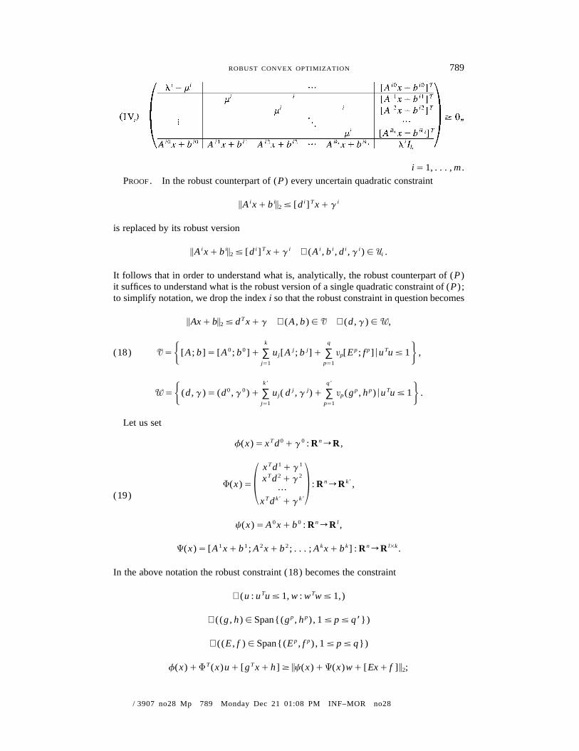
iÅ 1, . . . , m .PROOF. In the robust counterpart of (P) every uncertain quadratic constraint

i i i T i\A x/ b \ ° [d ] x/ g2

is replaced by its robust version

i i i T i i i i i\A x/ b \ ° [d ] x/ g ∀(A , b , d , g )√ U .2 i

It follows that in order to understand what is, analytically, the robust counterpart of (P)it suffices to understand what is the robust version of a single quadratic constraint of (P) ;to simplify notation, we drop the index i so that the robust constraint in question becomes

T\Ax/ b\ ° d x/ g ∀(A , b)√ V ∀(d , g)√W,2

k q0 0 j j p p TVÅ [A ; b]Å [A ; b ]/ u [A ; b ]/ £ [E ; f ]Éu u° 1 ,(18) ∑ ∑j pH J

jÅ1 pÅ1

k= q =0 0 j j p p TWÅ (d , g)Å (d , g )/ u ( d , g )/ £ (g , h )Éu u° 1 .∑ ∑j pH J

jÅ1 pÅ1

Let us set

T 0 0 nf(x)Å x d / g : R r R ,

T 1 1x d / gT 2 2x d / g n k=F(x)Å : R r R ,

(19)???1 2

T k= k=x d / g

0 0 n lc(x)Å A x/ b : R r R ,

1 1 2 2 k k n l1kC(x)Å [A x/ b ; A x/ b ; . . . ; A x/ b ] : R r R .

In the above notation the robust constraint (18) becomes the constraint

T T∀(u : u u° 1, w : w w° 1,)

p p∀((g , h)√ Span{(g , h ) , 1° p° q *})

p p∀((E , f )√ Span{(E , f ) , 1° p° q})

T Tf(x)/F (x)u/ [g x/ h]¢ \c(x)/C(x)w/ [Ex/ f ]\ ;2



The latter constraint is equivalent to the system of constraints (Iip) , p Å 1, . . . , q , ( IIip) ,p Å 1, . . . , p * and the following constraint:

∃l:

T Tf(x)/F (x)u¢ l ∀u , u u° 1,(20)

Tl¢ \c(x)/C(x)w\ ∀w , w w° 1.2

A pair (x , l) satisfies (20) if and only if it satisfies (IIIi ) along with the constraints

l¢ 0(21)

and

2 2 Tl ¢ \c(x)/C(x)w\ ∀w , w w° 1.(22) 2

The constraint (22) is equivalent to the constraint

T 2 2 2 2∀(( t , w) , w w° t ) : l t ¢ \c(x) t/C(x)w\ .(23) 2

In other words, a pair (x , l) satisfies (21), (22) if and only if l is nonnegative, andnonnegativity of the quadratic form ( t20 wTw) of the variables t , w implies nonnegativityof the quadratic form

2 2 2l t 0 \c(x) t/C(x)w\2

of the same variables. By Lemma 3.1, the indicated property is equivalent to the existenceof a nonnegative n such that the quadratic form

2 2 2 2 TW ( t , w)Å l t 0 \c(x) t/C(x)w\ 0 n( t 0w w)2

is positive semidefinite. We claim that n can be represented as ml with some nonnegativem, m Å 0 in the case of l Å 0. Indeed, our claim is evident if l ú 0. In the case of l Å0 the form W ( t , w) clearly can be positive semidefinite only when n Å 0 (look whathappens when w Å 0), and we indeed have n Å ml with m Å 0.

We have demonstrated that a pair (x , l) satisfies (21), (22) if and only if there existsa m such that the triple (x , l, m) possesses the following property

(p) : l, m ¢ 0; m Å 0 when l Å 0; the quadratic form

t2 T T TW ( t , w) Å l(l 0 m) t / lmw w 0 ( t w )R (x)R(x) ,S Dw

R(x) Å [c(x) ; C(x)] ,

of t , w is positive semidefinite.Now let us prove that the property (p) of (x , l, m) is equivalent to positive semidefinite-ness of the matrix S Å S(x , l, m) in the left hand side of (IVi ) .



Indeed, if l ú 0, positive semidefiniteness of W is equivalent to positive semidefinite-ness of the quadratic form

t2 T T T 01(l 0 m) t / mw w 0 ( t w )R (x)(lI ) R(x) ,l S Dw

which, via Schur complement, is exactly the same as positive semidefiniteness of S(x , l,m) . Of course, the matrix in the left-hand side of (IVi ) can be positive semidefinite onlywhen l å l i , m å mi are nonnegative. Thus, for triples (x , l, m) with l ú 0 the property(p) indeed is equivalent to positive semidefiniteness of S(x , l, m) . Now consider the caseof l Å 0, and let (x , l Å 0, m) possesses property (p) . Due to (p) , m Å 0 and W ispositive semidefinite, which for l Å 0 is possible if and only if R(x) Å 0; of course, inthis case S(x , 0, 0) is positive semidefinite. Vice versa, if l Å 0 and S(x , l, m) is positivesemidefinite, then, of course, R(x) Å 0 and m Å 0, and the triple (x , l, m) possessesproperty (p) .

The summary of our equivalences is that x satisfies (18) if and only if it satisfies (Iip) ,(IIip) for all possible p and there exist l Å l i , m Å mi such that the pair (x , l) satisfies(IIIi ) and the triple (x , l, m) satisfies (IVi ) . This is exactly the assertion of the theo-rem. h

3.4. Robust semidefinite programming. Next we consider uncertain SemidefiniteProgramming (SDP) problems.

An uncertain SDP problem is

nT 0 i l(P) Å min c x : A(x) å A / x A √ S ,(24) ∑ i /H H JJ

iÅ1 (A,b )√U

where is the cone of positive semidefinite l 1 l matrices and A 0 , A 1 , . . . , An belonglS/to the space S l of symmetric l 1 l matrices. This is a particular case of (4) correspondingto

l 0 1 n l nK Å S , z Å (A , A , . . . , A ) √ A Å (S ) ,/

nn 0 iX Å R , F(x , z) Å A / x A .∑ i

iÅ1

As before, we are interested in ellipsoidal uncertainties, but a general-type uncertaintyof this type turns out to be too complicated.

3.4.1. Intractability of the robust counterpart for a general-type ellipsoidal uncer-tainty. We start with demonstrating that a general-type ellipsoidal uncertainty affectingeven b only leads to computationally intractable (NP-hard) robust counterpart. To see it,note that in this case already the problem of verifying robust feasibility of a given can-didate solution x is at least as complicated as the following problem:

(*) Given k l 1 l symmetric matrices A 1 , . . . , Ak , (k is the dimension of the uncertaintyellipsoid) , check whether ui A i ° Il ∀(u √ R k : uTu ° 1).k( iÅ1

In turn, (*) is the same as the problem



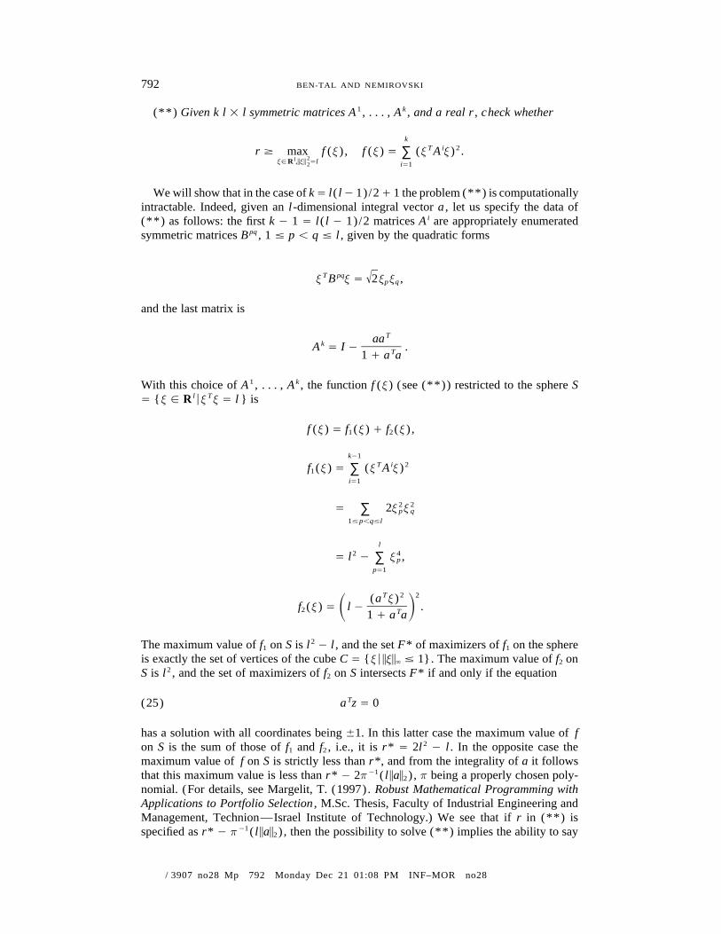
(**) Given k l 1 l symmetric matrices A 1 , . . . , Ak , and a real r , check whether

kT i 2r ¢ max f (j) , f (j) Å (j A j) .∑

2lj√R ,\j\ Ål2 iÅ1

We will show that in the case of kÅ l( l0 1)/2/ 1 the problem (**) is computationallyintractable. Indeed, given an l-dimensional integral vector a , let us specify the data of(**) as follows: the first k 0 1 Å l( l 0 1)/2 matrices Ai are appropriately enumeratedsymmetric matrices Bpq , 1 ° p õ q ° l , given by the quadratic forms

_√T pqj B j Å 2j j ,p q

and the last matrix is

TaakA Å I 0 .T1 / a a

With this choice of A 1 , . . . , Ak , the function f (j) (see (**)) restricted to the sphere SÅ {j √ R l

ÉjTj Å l } is

f (j) Å f (j) / f (j) ,1 2

k01T i 2f (j) Å (j A j)∑1

iÅ1

2 2Å 2j j∑ p q

1°põq°l

l2 4Å l 0 j ,∑ p

pÅ1

T 2 2(a j)f (j) Å l 0 .2 S DT1 / a a

The maximum value of f1 on S is l 2 0 l , and the set F* of maximizers of f1 on the sphereis exactly the set of vertices of the cube C Å {jÉ\j\` ° 1}. The maximum value of f2 onS is l 2 , and the set of maximizers of f2 on S intersects F* if and only if the equation

Ta z Å 0(25)

has a solution with all coordinates being {1. In this latter case the maximum value of fon S is the sum of those of f1 and f2 , i.e., it is r* Å 2l 2 0 l . In the opposite case themaximum value of f on S is strictly less than r*, and from the integrality of a it followsthat this maximum value is less than r* 0 2p01( l \a\2) , p being a properly chosen poly-nomial. (For details, see Margelit, T. (1997). Robust Mathematical Programming withApplications to Portfolio Selection , M.Sc. Thesis, Faculty of Industrial Engineering andManagement, Technion—Israel Institute of Technology.) We see that if r in (**) isspecified as r* 0 p01( l \a\2) , then the possibility to solve (**) implies the ability to say



whether the equation (25) has a solution with entries {1. The latter problem is known tobe NP-complete. h

In spite of the last intractability result there are interesting ‘‘well-structured’’ uncer-tainty ellipsoids which do lead to computationally tractable robust counterparts. An ex-ample of this type is discussed next.

3.4.2. ‘‘Rank 2’’ ellipsoidal uncertainty and robust truss topology design. Considera ‘‘nominal’’ (certain) SDP problem

0 T 0 l(p ) : min{c x : A (x) √ S };(26) /

here x is n-dimensional design vector and A 0(x) is l 1 l matrix affinely depending on x .Let d be a fixed nonzero l-dimensional vector; let us call rank 2 perturbation of A 0(·)associated with d a perturbation of the form

0 0 T TA (x) ° A (x) / b(x)d / db (x) ,

where b(x) is an affine function of x taking values in R l . Now consider the uncertainSDP problem (P) obtained from (p 0) by all possible perturbations associated with a fixedvector d x 0 and with b(·) varying in a (bounded) ellipsoid:

Tk kT 0 j T j(27) (P)Å min c x : A (x)/ u b ( x) d / d u b ( x) ¢ 0 ;∑ ∑j jH H F G F G JJ

k TjÅ1 jÅ1 u√R :u u°1

here b j( x) are given affine functions of x taking values in R l .

PROPOSITION 3.1. The robust counterpart (P*) of the uncertain SDP problem (P) isequivalent to the following SDP problem :

T(P) min c x

nw .r .t . x √ R , l √ R subject to(28)

1 2 k TlI [b (x) ; b (x) ; . . . ; b (x)]k(a) ¢ 0.S D1 2 k 0 T[b (x) ; b (x) ; . . . ; b (x)] A (x) 0 ldd

PROOF. Let

1 2 kb(x) Å [b (x) ; b (x) ; . . . ; b (x)] ;

a vector x is feasible for (P*) if and only if

l k T T 0 T T T∀(j √ R ) ∀(u √ R , u u ° 1): j A (x)j / 2(d j)(u b (x)j) ¢ 0,(29)

or equivalently, if and only if

l T 0 T T∀(j √ R ) : j A (x)j 0 2Éd jÉ\b (x)j\ ¢ 0.(30) 2



Condition (30), in turn, is equivalent to the following one:

l k T 2 T∀(j √ R , h √ R ) : P(j, h) å (d j) 0 h h ¢ 0 c

(31)T 0 T TQ(j, h) å j A (x)j / 2h b (x)j ¢ 0.

According to Lemma 3.1, (31) is equivalent to the existence of a nonnegative l such thatthe quadratic form

Q(j, h) 0 lP(j, h)

of j, h is positive semidefinite. Summarizing our observations, we see that x is feasiblefor (P*) if and only if there exists l ¢ 0 such that the matrix

TlI b (x)kS D0 Tb(x) A (x) 0 ldd

is positive semidefinite. h

The situation described in Proposition 3.1 arises, e.g., in the truss topology designproblem described in Introduction (see Ben-Tal and Nemirovski 1997 for more details) .In the latter problem, the ‘‘nominal’’ program (26) is of the form

min ts.t.

the design vector being ( t1 , . . . , tp , t) ; ti are bar volumes, t represents the compliance,and f is the ‘‘nominal’’ external load. In the robust setting of the TTD problem, we replacethe nominal load f with an ellipsoid of loads centered at f ; this is nothing but rank 2perturbation of the nominal problem associated with d Å e1 and a properly chosen bi(x)( in fact, independent of x) .

3.4.3. ‘‘Approximate’’ robust counterpart of an uncertain SDP problem. As wehave seen, an uncertain SDP problem with a general-type ellipsoid U may result in acomputationally intractable robust counterpart. This can occur in other situations as well,and whenever this is the case, a natural way to overcome the difficulty is to replace therobust counterpart by a ‘‘tractable approximation.’’ Let us start with introducing this latterconcept.

Approximation of the robust counterpart. Consider an uncertain optimizationproblem:

T0(P) Å {min{c x : F(x , z) √ K , x √ X}} ,z√z /V



where z0 is the ‘‘nominal’’ data and V is a convex ‘‘perturbation set’’ containing 0. Let

T 0(P*) min{c x : x √ X, F(x , z) √ K ∀z √ z / rV}r

be the robust counterpart of the uncertain problem obtained from (P) by replacing the originalperturbation set V by its r-enlargement, and let G˙(r) denote the feasible set of (P*).r

DEFINITION 3.1. We say that a ‘‘certain’’ optimization problem

T /(P) : min{c x : (x , l) √ X }

with design variables x , l and feasible domain X / is an approximation of the robustcounterpart (P*) å of (P) , if the projection G/(P) of the feasible set of (P) on*(P )1

the plane of x-variables is contained in the feasible set G˙(1) of the robust counterpart(P*), i .e ., if (P) is ‘‘more conservative’’ than the robust counterpart of (P) .

A natural ‘‘measure of conservatism’’ of (P) as an approximation to (P*) is as follows:

/cons(P) Å inf{r ¢ 1 : G˙(r) , G (P)}.

DEFINITION 3.2. We say that (P) is an a-conservative approximation of (P*), ifcons(P) ° a, i .e ., if

/x √ G (P) c x √ G*(1),H /x /√ G (P) c x /√ G˙(r) ∀r ú a.

Note that from the viewpoint of practical modeling it is nearly the same to use the exactrobust counterpart or its approximation with ‘‘moderate’’ level of conservativeness.Therefore, if the exact counterpart turns out to be a ‘‘computationally bad’’ problem (asit is the case for uncertain SDP problems with ellipsoidal uncertainties) , it makes senseto look for an approximate counterpart which is on one hand with a ‘‘reasonable’’ levelof conservativeness and on the other hand is computationally tractable. We now presenta result in this direction.

A ‘‘universal’’ approximate robust counterpart to an uncertain SDP prob-lem. Consider an uncertain SDP problem in the form

T i li i i0(P) Å {min{c x : A (x) √ S , i Å 1, . . . , m}} ,/ A (·)√A (·)/V ,iÅ1, . . . , mi

A i0(·) being an affine mapping from R n to and Vi , 0 √ Vi , being convex perturbationliSsets in the spaces of mappings of this type.

Assume that(#) . For every i°m the set Vi can be approximated ‘‘up to factor gi ’’ by an ellipsoid,

i.e., we can find out ki affine mappings A ij(·) : R n r j Å 1, . . . , ki , in such a wayliS ,that ⊆ Vi ⊆ where0 0V g V ,i i i

ki0 ij TV Å u A (·)Éu u ° 1 .∑i jH J

jÅ1



THEOREM 3.4. Under assumption (#) the SDP program

Tmin c x(P) : x

s .t .

i0 i1 i2 ikiA (x) g A (x) g A (x) ??? g A (x)i i ii1 i0g A (x) A (x)ii2 i0B (x) å g A (x) A (x) ¢ 0, i Å 1, . . . , m .i i

?: ???1 2??ik i0ig A ??? A (x)i

is an a-conservative approximate robust counterpart of (P) with__ __√ √

a Å max g min[ k , l ] .(32) i i iiÅ1, . . . , m

Note that the strength of the result is in the fact that the guaranteed level of conservatisma is proportional to the minimum of the square roots of the dimensions maxi ki andmaxi li .

PROOF OF THE THEOREM. We should prove that ( i) (P) indeed is an approximaterobust counterpart of (P) , and that ( ii ) the level of conservativeness of (P) is as givenin (32).

( i ) Assume that x is feasible for (P) , and let us prove that x is robust feasible for(P) . To this end it suffices to verify that for every i Å 1, . . . , m one has

i0B (x) ¢ 0 c A (x) / A(x) ¢ 0 ∀A √ V .(33) i i

To simplify notation, let us drop the index i and write A 0 Å A i0(x) , A j Å A ij( x) , gÅ gi , etc.

Assume that Bi (x) ¢ 0. The matrix A 0 clearly is positive semidefinite. Let B be apositive definite symmetric matrix such that B ¢ A 0 ; then the matrix

1 2 kB gA gA ??? gA1gA B2B Å gA B

?: ???1 2??kgA ??? B

is positive semidefinite, i.e., for every collection of vectors j, h1 , h2 , . . . , hk one has

k kT T T jj Bj / h Bh / 2g j A h ¢ 0.∑ ∑j j j

jÅ1 jÅ1

Minimizing the left-hand side of this equation in h1 , . . . , hk , we get

kT 2 T j 01 jj Bj 0 g j A B A j ¢ 0 ∀j,∑

jÅ1



or, denoting Dj Å B01/2A jB01/2 ,

k2 2g D ° I .(34) ∑ j l

jÅ1

Now let A(·) √ Vi and let A Å A(x) ; note that in view of (#)

kT 2 j∃(u , u u ° g ) : A Å u A .∑ j

jÅ1

For an arbitrary h √ R l , we have

kT T j

Éh AhÉ ° Éu ÉÉh A hÉ∑ j

jÅ1

_____ ___________√ √k k

2 T j 2° u (h A h)∑ ∑j

jÅ1 jÅ1

______________________√k

1/2 T 01/2 j 2° g [(B h) (B A h)]∑jÅ1

_____________________√k

T T j 01 j° g [h Bh][h A B A h]∑jÅ1

_______________________√k

T T 1/2 2 1/2Å g [h Bh][h B D B h]∑ j

jÅ1

T° h Bh

[we have used (34)] .

Thus,

T TÉh AhÉ ° h Bh ∀h.

This relation is valid for all positive definite matrices B which are ¢A 0 , so that A 0 / A¢ 0. Since the latter inequality is valid for all A Å A(x) , A(·) √ Vi , x indeed satisfiesthe conclusion in (33). ( i ) is proved.

( ii ) Assume that x √ G˙(a) with a given by (32); we should prove that x is feasiblefor (P) . Arguing by contradiction, assume that x is not feasible for (P) . First of all, wenote that all A i0(x) are positive semidefinite—otherwise x would not be feasible evenfor the nominal instance and therefore would not belong to G˙(a) . Since x is not feasiblefor (P) , there exists i such that the matrix Bi (x) is not positive semidefinite. Choosingas B a positive definite matrix which is ¢Ai0(x) and is close enough to Ai0(x) , we seethat the matrix



i1 i2 ikiB g A (x) g A (x) ??? g A (x)i i ii1g A (x) Bii2B Å g A (x) Bi

???? ???1 2??ikig A Bi

is not positive semidefinite.In view of the same reasoning as in the proof of (i) , the latter fact means exactly that

the matrix

k2 2 01/2 j 01/2I 0 g D , D Å B A B ,∑l j j

jÅ1

is not positive semidefinite (we use the same shortened notation as in the proof of (i)) .In other words, there exists a vector h , hTh Å 1, such that

kTh h ú 1,∑ j j

jÅ1

h Å gD h , j Å 1, 2, . . . , k .(35)

j j

We claim that

kT 2∃u : {u u Å a } & {\D\ ú 1}, D Å u D ,(36) ∑ j j

jÅ1

where \·\ is the operator norm of a symmetric matrix.Indeed, consider two possible cases: (a) k å ki ° l å li , and (b) k ú l .Assume that (a) is the case. It is evident that one can choose numbers ej Å {1 in such

a way that

k k2Te h ¢ h h [ú1],∑ ∑j j j ji i

jÅ1 jÅ12

whence

2kT 02h e D h ú g .∑ j jF G

jÅ1

In view of this inequality, setting uj Å aejk01/2 , j Å 1, . . . , k , we satisfy the first relationin the conclusion of (36), and the operator norm of the corresponding matrix D2 isúa 2g02k01 ; the latter quantity is ¢1, since in case (a) one clearly has a ¢ gk 1/2 , see(32). Thus, \D\ 2 ¢ \D 2\ ú 1, as required in (36).

Now consider case (b) . Denoting by dp the p th coordinate of an l-dimensional vectord and taking into account that in view of (35) one has



k lp 2(h ) ú 1,∑ ∑ j

jÅ1 pÅ1

we immediately conclude that there exists an index q √ {1, 2, . . . , l } such that

kq 2 01(h ) ú l .∑ j

jÅ1

Consequently, there exists a vector u √ R k , uTu Å a 2 , such that

kq 01/2u h ú al ,∑ j j

jÅ1

or, which is the same,

kq 01 01/2u ( D h) ú ag l ¢ 1.∑ j j

jÅ1

(We have taken into account that in case (b), due to the origin of a, the quantity ag01l01/2

is ¢ 1.) In other words, u satisfies the conclusion in (36) (recall that hTh Å 1).Now let u , D be given by (36) (we just have seen that this relation is always true) ,

and let A Å ujA j , so that D Å B01/2AB01/2 . Since \D\ ú 1, at least one of thek( jÅ1

matrices Il { D is not positive semidefinite, or, which is the same, at least one of thematrices B { A is not positive semidefinite. On the other hand, uTu ° a 2 , and therefore(see (#)) { ujA ij(·))√ aVi ; since x was assumed to belong to G˙(a ) , the matricesk(( jÅ1

Ai0 { A should be positive semidefinite; due to B ¢ Ai0 , it implies also positive semi-definiteness of the matrices B { A , and we come to the desired contradiction. h

REMARK 3.1. In connection with Assumption (#) it is worth noting that , in the casewhen V is the intersection of k ellipsoids centered at the origin , this assumption is satisfiedwith g Å Indeed , we may assume that the ellipsoids in question are E i

_√k .

Å ° 1}; their intersection clearly contains the ellipsoid {zÉzTT k T{zÉzQ Q z ( Q Q zi i iÅ1 i i

° 1} and is contained in a times larger ellipsoid ._√k

3.5. Affinely parameterized uncertain programs. Consider the case of an uncertainproblem with affine uncertainty and K Å mR :/

T j(P) Å {min{c x : x √ X, f (x , z) ¢ 0, i Å 1, . . . , m}} ,i zÅ{z } √Ui, ji

where

kj j0f (x , z) Å f (x) / z f (x) .∑i i i i

jÅ1

The robust counterpart of (P) is the problem

(P*)

Tmin c x

F (x) ¢ 0, i Å 1, . . . , m ,i



where

kj j0F (x) Å inf f (x) / z f (x) .∑i i i iF Gj

zÅ{z }√Ui jÅ1

Assume that the uncertainty set U is a bounded ellipsoid, i.e., the image of the unit Eu-clidean ball under affine mapping:

0 l TU Å {z Å z / PuÉu √ R , u u ° 1}.(37)

Our goal is to demonstrate that in the case in question the robust counterpart is basically‘‘as computationally tractable’’ as the instances of our uncertain program.

Indeed, let us look what is the robust version of a single uncertain constraint. Droppingthe index i , we write the uncertain constraint and its robust version, respectively, as

1f (x)2f (x)0 T0 ° f ( x , z) å f (x) / z f ( x) , f ( x) Å ,(38)???1 2kf (x)

0 ° F(x) å min f ( x , z) .z√U

We immediately see that

_____________√0 0 T T TF(x) Å f (x) / (z ) f ( x) 0 f (x)PP f ( x) .

Note also that F is concave on X (recall that we always assume that the mapping F(x , z)is K-concave in x √ X) . Thus, in the case under consideration the robust counterpart isan ‘‘explicitly posed’’ convex optimization program with constraints of the same ‘‘levelof computability’’ as the one of the constraints of the instances. At the same time, theconstraints of the robust counterpart may become worse than those of the instances, e.g.,they may lose smoothness.

There are, however, cases when the robust counterpart turns out to be of the sameanalytical nature as the instances of the uncertain program in question.

Example: A simple uncertain geometric programming problem. Consider the caseof an uncertain geometric programming program in the exponential form with uncertaincoefficients of the exponential monomials, so that the original constraints are of the form

kj T0 ° f ( x , z) Å 1 0 z exp{[b ] x}(39) ∑ j

jÅ1

(b j are ‘‘certain’’) and the uncertainty ellipsoid, for every constraint, is contained in thenonnegative orthant and is given by (37). Here the robust version of (39) is the constraint

k _____________√0 j T T T0 ° F(x) å 1 0 z exp{[b ] x} 0 f (x)PP f(x) ,∑ j

jÅ1

1 T 2 T k T Tf(x) Å (exp{[b ] x} exp{[b ] x}···exp{[b ] x}) .(40)



Under the additional assumption that the matrix PPT is a matrix with nonnegativeentries, we can immediately convert (40) into a pair of constraints of the same form as(39); to this end it suffices to introduce for each constraint an additional variable t andto represent (40) equivalently by the constraints

k0 j T0 ° 1 0 z exp{[b ] x} 0 exp{ t},∑ j

jÅ1

kT p q T0 ° 1 0 (PP ) exp{[b / b ] x 0 2t}.∑ pq

p,qÅ1

Thus, in the case under consideration the robust counterpart is itself a geometric program-ming program.

4. Saddle point form of programs with affine uncertainty. Consider once again anuncertain Mathematical Programming problem with affine uncertainty and K Å mR :/

kjT i 0 i(P) Å min c x : x √ X, f (x , z ) å f (x) / z f (x) ¢ 0,∑i i j iH H

jÅ1

i Å 1, 2, . . . , m ,JJiz √U ,iÅ1, . . . ,mi

each Ui being a closed convex set in some Note that in the case in question As-kiR .sumption A becomes

A.1. X is a closed convex set with a nonempty interior , the functions are con-jf (x)i

tinuous on X, i Å 1, . . . , m , j Å 1, . . . , k , and the functions fi (x , z i) are concave in x√ X for every z i √ Ui , i Å 1, . . . , m .

The robust counterpart of (P) is the problem

(P*)

Tmin c x

F (x) ¢ 0, i Å 1, . . . , m ,i

kj0 iF (x) Å inf f (x) / z f (x) .∑i i j iF G

iz √Ui jÅ1

which is equivalent to the problem

mTmin sup c x 0 l F (x) ,∑ i iH J

mx√X l√R/ iÅ1



or explicitly the problem

m kjT 0 imin c x 0 inf l f (x) / l z f (x) .(41) ∑ ∑i i i j iH F GJ

i mx√X z √U ,l√Ri /iÅ1 jÅ1

Now let us set

kj k/1

Pf (x , h) Å h f (x) : X 1 R r R ,∑i j i

jÅ0

i i i T iW Å cl{(m, mz , mz , . . . , mz ) Ém ¢ 0, z √ U };i 1 2 k i

note that Wi is a closed convex cone in R k/1 . We clearly have

kj0 i i

Pinf l f (x) / l z f (x) Å inf f (x , h ) ,∑i i i j i iF Gi iz √U ,l¢0 h √Wi i ijÅ1

so that the problem (41) is exactly the problem

mT i

Pmin c x 0 inf f (x , h ) .(42) ∑ iH Jix√X h √WiiÅ1

Now let

m

W Å W ,∏ i

iÅ1

1 mh Å (h , . . . , h ) ,

mT i

PL(x , h) Å c x 0 f (x , h ) : X 1 W r R .∑ i

iÅ1

Due to A.1 and to the origin of W, the function L is convex in x √ X for every h √ Wand affine (and therefore concave) in h. We summarize the above facts in

PROPOSITION 4.1. Under assumption A.1 , the robust counterpart (P*) of uncertainproblem (P) is equivalent to the saddle point problem

min sup L(x , h)(43)x√X h√W

with convex-concave and continuous on X 1 W function L(x , h) .The latter result provides us with an opportunity to handle the uncertain problem underconsideration via its dual problem

max inf L(x , h)h√W x√X

which in some cases may be better suited for a numerical solution. Another advantage ofthe saddle point formulation of the robust counterpart is seen from the following consid-



FIGURE 2. A simple circuit.

erations. In simple enough cases (cf. §3.5) we can explicitly perform the inner maximi-zation in h in (43) and end up with an explicit optimization form of the robust counterpart:

P Pmin L(x) L(x) Å sup L(x , h) .(44) F Gx√X h√W

We point out, however, that sometimes this policy, even when it can be carried out, isnot necessarily the best one; there are cases when, computationally, it is preferable towork directly on the saddle point form of the robust counterpart than on its optimizationform. The reason is that in the case when possess nice analytical structure, the functionjf i

L(x , h) basically inherits this nice structure, and in favourable circumstances we can solvethe saddle point problem by advanced interior point methods for variational inequalities(see Nesterov and Nemirovski 1994, Chapter 7) . In contrast to this, the objective in theoptimization program (44), even if it can be explicitly computed, typically is much worseanalytically than the functions it may, e.g., loose smoothness even when all functionsjf ;i

are very smooth. As a result, it may happen that the only numerical methods whichjf i

can be used to solve (44) directly are relatively low-performance ‘‘black box’’-orientedtools of nonsmooth convex optimization, like the bundle methods, the Ellipsoidmethod, etc.

To illustrate the point, let us consider the following simple example:

Heat dissipation problem. Consider an electric circuit (see Figure 2) represented asa connected oriented graph G with N arcs, an arc ( ij) possessing a given conductance sij

√ (0, `) . Assume that the arcs of the circuit are charged with external constant voltagesyij , and the vector y of these voltages is restricted to belong to a given convex and compactset Y. The voltages induce currents in the circuit; as a result, the circuit dissipates heat.According to Kirchoff ’s laws, the heat dissipated by the circuit per unit time is

TH Å min (Qu / Py) S(Qu / Py) ,Mu√R

where Q and P are some matrices given by the topology of the circuit, M is the numberof nodes of the circuit and S is N 1 N diagonal matrix with the diagonal entries indexedby the arcs of G and equal to sij . The problem is to choose y √ Y which minimizes thedissipated heat:

T(p) min t : t 0 min (Qu / Py) S(Qu / Py) ¢ 0 ,H JmxÅ( t,y)√XÅR1Y u√R



the data in the problem being the conductances sij , or, which is the same, the diagonalpositive semidefinite matrix S . In fact, in what follows we treat the more general problemwhere S is symmetric positive semidefinite, but not necessarily diagonal.

Now assume that the data are uncertain: all we know is that S √ U, U being a closedconvex subset of the positive semidefinite cone for the sake of simplicity, we assumeNS ;/that U is bounded. The saddle point problem (43) becomes here

Tmin sup t(1 0 l) / l min(Qu / Py) S(Qu / Py) .F G( t,y)√X l¢0,S√U u

It is clearly seen that the latter problem is equivalent to the saddle point problem

Tmin max min(Qu / Py) S(Qu / Py) ,F Gy√Y S√U u

which in turn is equivalent to the saddle point problem

Tmin max f ( y , u ; S) , f ( y , u ; S) Å (Qu / Py) S(Qu / Py) .(45)y√Y, u S√U

(We have used the standard min-max theorem (see Rockafellar 1970) and have takeninto account that U , so that the function (Qu / Py)TS(Qu / Py) is convex in (y ,NS ,/u) for every S √ U and is linear, and therefore concave, in S .)

The nice analytical structure of f makes it possible to solve the saddle point problemby the polynomial time path-following interior point methods from (Nesterov and Nem-irovski 1994, Chapter 7) provided that the convex sets Y, U are ‘‘simple’’—admit explicitself-concordant barriers. Thus, here the saddle point form of the robust counterpart yieldsa problem which can be solved by theoretically efficient interior point methods. This isnot always the case for the optimization form (44) of the robust counterpart. Indeed,consider the simplest case where Q is the zero matrix (such a case has no actual sense inthe Heat Dissipation problem, but it makes sense mathematically, which is sufficient toillustrate the point) . In this case the objective L(x) , x Å ( t , y) in problem (44) becomes

T T/` , t õ max y P SPy ,S√UH

t , otherwise

so that (44) is nothing but the problem

T Tmin F(y) , F(y) Å max y P SPy .(46)y√Y S√U

Now assume that U , is an ellipsoid:NS/

k0 j TU Å S / £ S É£ £ ° 1 .∑ jH J

jÅ1

Then the objective F in (46) can be explicitly computed:

______________√k

T T T T j 2F(x) Å x P SPx / (x P S Px) .(47) ∑jÅ1



Note that since not all S j necessarily are positive semidefinite, it is not even seen from(47) that F is convex. Moreover, direct minimization of convex functions of the type(47), where not all S js are positive semidefinite, is not as yet covered by the currentinterior point methodology.

Acknowledgment. The research was supported by the Israel Science Foundation grant# 306/94-3, by the Fund for the Promotion of Research at Technion, by the G.I.F. contractNo. I-0455-214.06/95 and by the Israel Ministry of Science grant # 9636-1-96.

ReferencesBen-Tal, A., A. Nemirovski. 1995a. Robust solutions to uncertain linear problems. Research Report # 6/95,

Optimization Laboratory, Faculty of Industrial Engineering and Management, Technion—the Israel In-stitute of Technology, Technion City, Haifa 32000, Israel., . 1995b. Robust Convex Programming. Working paper, Faculty of Industrial Engineering andManagement, Technion—the Israel Institute of Technology, Technion City, Haifa 32000, Israel., . 1997. Robust truss topology design via semidefinite programming. SIAM J . Optim . 7 991–1016.

Boyd, S., L. El Ghaoui, E. Feron, V. Balakrishnan. 1994. Linear Matrix Inequalities in System and ControlTheory , Society of Industrial and Applied Mathematics, Philadelphia.

El-Ghaoui, L., H. Lebret. 1996. Robust solutions to least-square problems with uncertain data matrices. Workingpaper, Ecole Nationale Superieure De Techniques Avancees, 32, Bd. Victor, 75739 Paris, France.

Falk, J. E. 1976. Exact solutions to inexact linear programs. Oper . Res . 34 783–787.Kouvelis, P., G. Yu. 1997. Robust Discrete Optimization and Its Applications . Nonconvex Optimization and Its

Applications 14 . Kluwer Academic Publishers, Dordrecht, Germany.Mulvey, J. M., R. J. Vanderbei, S. A. Zenios. 1995. Robust optimization of large-scale systems. Oper . Res . 43

264–281.Nemirovski, A. 1997. On self-concordant convex-concave functions. Research Report # 3/97 (June 1997),

Optimization Laboratory Faculty of Industrial Engineering and Management, Technion—the Israel In-stitute of Technology, Technion City, Haifa 32000, Israel.

Nesterov, Yu., A. Nemirovski. 1994. Interior Point Polynomial Methods in Convex Programming . Society ofIndustrial and Applied Mathematics, Philadelphia.

Oustry, H., L. El Ghaoui, H. Lebret. 1996. Robust solutions to uncertain semidefinite programs. Working paper,Ecole Nationale Superieure De Techniques Avancees, 32, Bd. Victor, 75739 Paris, France. SIAM J .Optim . ( to appear) .

Rockafellar, R. T. 1970. Convex Analysis . Princeton University Press, Princeton, NJ.Singh, C. 1982. Convex programming with set-inclusive constraints and its applications to generalized linear

and fractional programming. JOTA 38 33–42.Soyster, A. L. 1973. Convex programming with set-inclusive constraints and applications to inexact linear

programming. Oper . Res . 21 1154–1157.Zhou, K., J. Doyle, K. Glover. 1995. Robust and Optimal Control . Prentice Hall, NJ.

A. Ben-Tal: Faculty of Industrial Engineering and Management, Technion—Israel Institute of Technology,Technion City, Haifa 32000, Israel; e-mail: [email protected]

A. Nemirovski: Faculty of Industrial Engineering and Management, Technion—Israel Institute of Technology,Technion City, Haifa 32000, Israel; e-mail: [email protected]

ROBUST CONVEX OPTIMIZATION - Atlanta, GAnemirovs/MOR_RCO_1998.pdf · We study convex optimization...

Documents

Transcript of ROBUST CONVEX OPTIMIZATION - Atlanta, GAnemirovs/MOR_RCO_1998.pdf · We study convex optimization...