Robust Control

References:

1. K. Zhou, and J. C. Doyle,Essentials of Robust Control,

Prentice-Hall, Inc., 1998

2. S. Skogestad, and I. Postlethwaite,Multivariable Feedback Control:

Analysis and Design, John Wiley & Sons Ltd., 1996

1

Introduction

1. Why Robust Control?Models are uncertain.

• Real environments of a control system may change and operatingconditions may vary from time to time.

• Even if the environment does not change, other factors are themodel uncertainties as well as noises.

• Any mathematical representation of a system often involvessimplifying assumptions. Nonlinearities are either unknown andhence unmodeled, or are modeled and later ignored in order tosimplify analysis. High frequency dynamics are often ignored atthe design stage as well.

In consequence, control systems designed based on simplifiedmodels may not work on real plants in real environments.

2

2. Robustness and Robust Control

• Robustness. The property that a control system must maintain

overall system performance despite changes in the plant is called

robustness. Any control system must possess this property for it

to operate properly in realistic situations.

Mathematically, this means that the controller must perform

satisfactorily not just for one plant, but for a family of plants. If a

controller can be designed such that the whole system to be

controlled remains stable when its parameters vary within certain

expected limits, the system is said to possess robust performance.

• Robust Control. The problem of designing controllers that satisfy

both robust stability and performance requirements is called

robust control.

3

3. Scope of Robust ControlSome of the key questions in robust control theory are:

1) Characterizing plant variation. In robust control theory, plant

variation plays a central role. What is a good way to describe

plant variations or uncertainty? Some descriptions attempt to

faithfully describe the variations that might be encountered (e.g.,

probability distributions on physical parameters). Other

descriptions are more convenient for the associated theory(e.g.,

bounds on singular values of transfer matrix errors).

2) Robustness analysis. Given a controller and plant, and some

description of the plant uncertainty, how can we determine such

things as “typical” or “worst-case” performance? How can we

predict the performance degradation caused by variation inthe

plant? How can we verify that some performance specifications

are met for some set of plants?

4

3) Robust controller synthesis. Given a plant and some descriptionof the plant uncertainty, how can we design a controller thatoptimizes “typical” or “worst-case” performance? How can wedesign a controller that meets some performance specificationsfor some set of plants (e.g., all or typical)?

It’s important to remember several things:

• First, these questions were asked, and partial answers obtained,before the term “robust control” was coined.

• Second, the qualifier “robust” shouldn’t be necessary sinceawell-designed controller must be able to tolerate the plantchanges or variations that can be expected. To put it anotherway,a controller that cannot tolerate variations in the plant that will beencountered in operation is simply a poorly-designed controller,not just a non-robust controller. (But the extra qualifier “robust”has helped re-focus attention on this important aspect of controlengineering.)

5

4. Development of Robust Control

• In classical control theory, gain and phase margins are usedtorepresent the robustness of a control system.

• During the development of state-space optimal control in 1960s,control system robustness received less attention, since the idea ofplant change, variation, or uncertainty played at best a secondaryrole.

– Some initial results showed that the state-feedbackimplementation of LQR was very tolerant of changes in theplant. This led to the hope that controllers designed to beoptimal for a fixed, known plant might automatically turn outto be robust, i.e., tolerant to changes in the plant. In a shortnote, Doyle pointed out that this is not the case.

• Robustness re-drew attention in 1980s. One of the most famouscontributions of robust control theory is the development of H∞

controller synthesis.

6

Contents

1. Norms of Signals and Systems

2. Uncertainty and Robustness

3. Performance Specifications

4. Robust Controller Synthesis

5. Model Reduction

6. Robustness Measure

7. Internal Model Control (IMC)

8. Wide-Range Robust Control

7

Chapter 1. Norms of Signals and Systems

A system can be regarded as a ‘gray box’ for manipulating signals. Todescribe the size of signals and systems, we need to work on functionspaces. There are two kinds of functions spaces that we are interested in:

• Linear spaces composed of real functions, especially, functions oftime f (t) with t ∈ R.

• Linear spaces composed of complex functionsF(s) with s∈ C.

Outline of this chapter:

• Vector Spaces

• Function spaces

• Norms of signals

• Norms of systems

8

1.1 Vector Spaces

Let F be a scalar field (it can be taken to be real numbersR, or thecomplex numbersC). SupposeV is a nonempty set, together with a set ofoperations: addition and scalar multiplication, then a linearvector spaceis the 4-tuple{V,F,+, ·} such that the following rules are satisfied for allx,y∈ V andα ,β ∈ F:

1) Commutativity:x+y= y+x

2) Associativity:(x+y)+z= x+(y+z)

α · (β ·x) = (αβ ) ·x

3) Identity: there exists an element 0∈ V and 1∈ F such that

x+0= x, 1·x= x

9

4) Inverse: x∈ V implies that there existsy∈ V such thatx+y= 0.

5) Distributivity:

α · (x+y) = α ·x+β ·y

(α +β ) ·x= α ·x+β ·x

Examples:

• Set of vectors (Rn) over the field of real numberR;

• Set of vectors (Cn) over the filed of complex numberC;

• Set of allm×n matrices (Cm×n) over the filed ofC.

• Set of all functions mapping fromR toRn ( f : R→ Rn) over the

fieldR.

10

1.1.1 Normed SpacesWe can define a norm on a vector space to denote the size of an element.

LetV be a vector space, a real-valued function‖ · ‖ : V→ R is said to be a

norm if it satisfies the following properties for anyx∈ V andy∈ V:

1) ‖x‖ ≥ 0 (positivity).

2) ‖x‖= 0 if and only ifx= 0 (positive definiteness).

3) ‖αx‖= |α |‖x‖ for any scalarα (homogeneity).

4) ‖x+y‖ ≤ ‖x‖+‖y‖ for anyx,y∈ V (triangular inequality).

A vector space together with a norm is called anormed spaceand is

denoted(V,‖ · ‖).A normed space iscompleteif every Cauchy sequence in it converges.

Such a space is referred to as aBanach space.

11

Vector Norms (Norms onCn)

For vector spaceCn, several norms can be defined:

• 1-norm.

‖x‖1 :=n

∑i=1

|xi |

• 2-norm.

‖x‖2 :=

√n

∑i=1

|xi |2

• ∞-norm.‖x‖∞ := max

1≤i≤n|xi |

They are special cases of thep-norm defined as

‖x‖p :=

(n

∑i=1

|xi |p)1/p

12

Matrix Norms ( Norms on Cm×n)

Let A∈ Cm×n, then theFrobenius norm of A is defined as

‖A‖F :=√

trace(A∗A) =

√m

∑i=1

n

∑j=1

|ai j |2

If we treatA as a linear transform fromCn toCm, then theinducedp-norm of A (induced by a vectorp-norm) is defined as

‖A‖p := supx 6=0

‖Ax‖p

‖x‖p

A most often used norm is the induced 2-norm (Euclidean norm).

‖A‖1 = maxj

m

∑i=1

|ai j |, ‖A‖∞ = maxi

n

∑j=1

|ai j |, ‖A‖2 = σmax(A)

From now on, if there is a norm without the subscript, then it refers to

(vector or matrix) 2-norm.

13

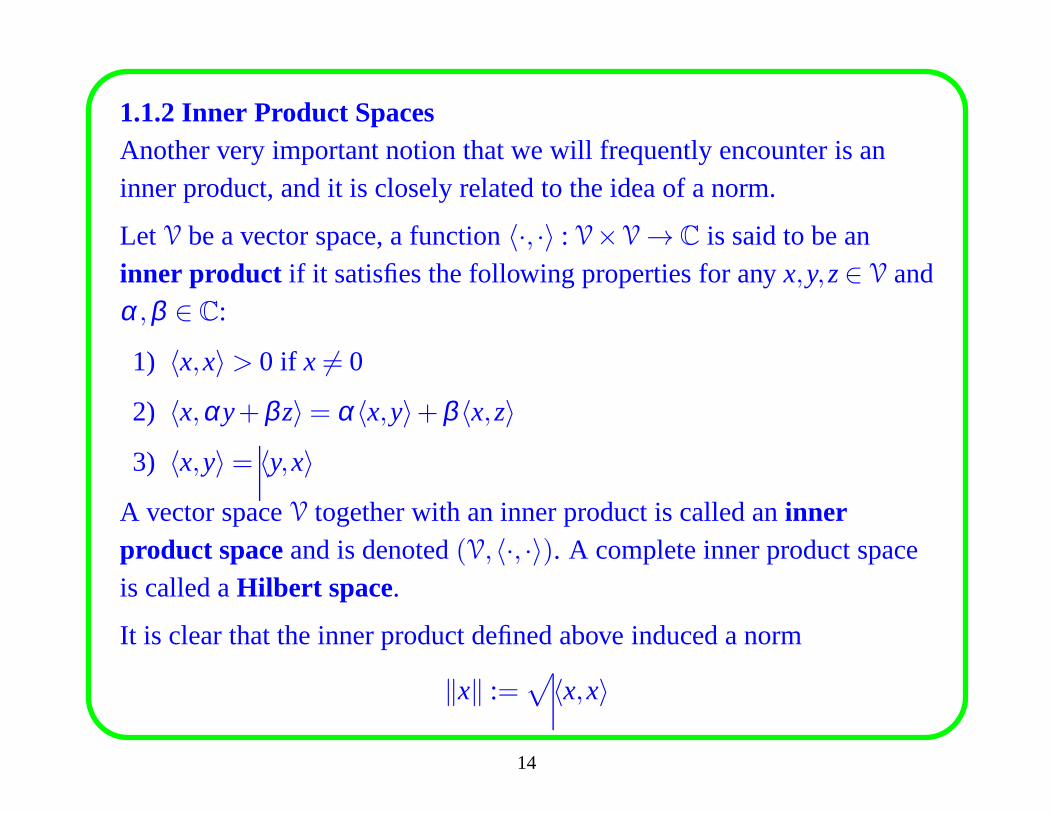
1.1.2 Inner Product SpacesAnother very important notion that we will frequently encounter is aninner product, and it is closely related to the idea of a norm.

Let V be a vector space, a function〈·, ·〉 : V×V→ C is said to be aninner product if it satisfies the following properties for anyx,y,z∈ V andα ,β ∈ C:

1) 〈x,x〉> 0 if x 6= 0

2) 〈x,αy+βz〉= α〈x,y〉+β 〈x,z〉3) 〈x,y〉= 〈y,x〉

A vector spaceV together with an inner product is called aninnerproduct spaceand is denoted(V,〈·, ·〉). A complete inner product spaceis called aHilbert space.

It is clear that the inner product defined above induced a norm

‖x‖ :=√

〈x,x〉

14

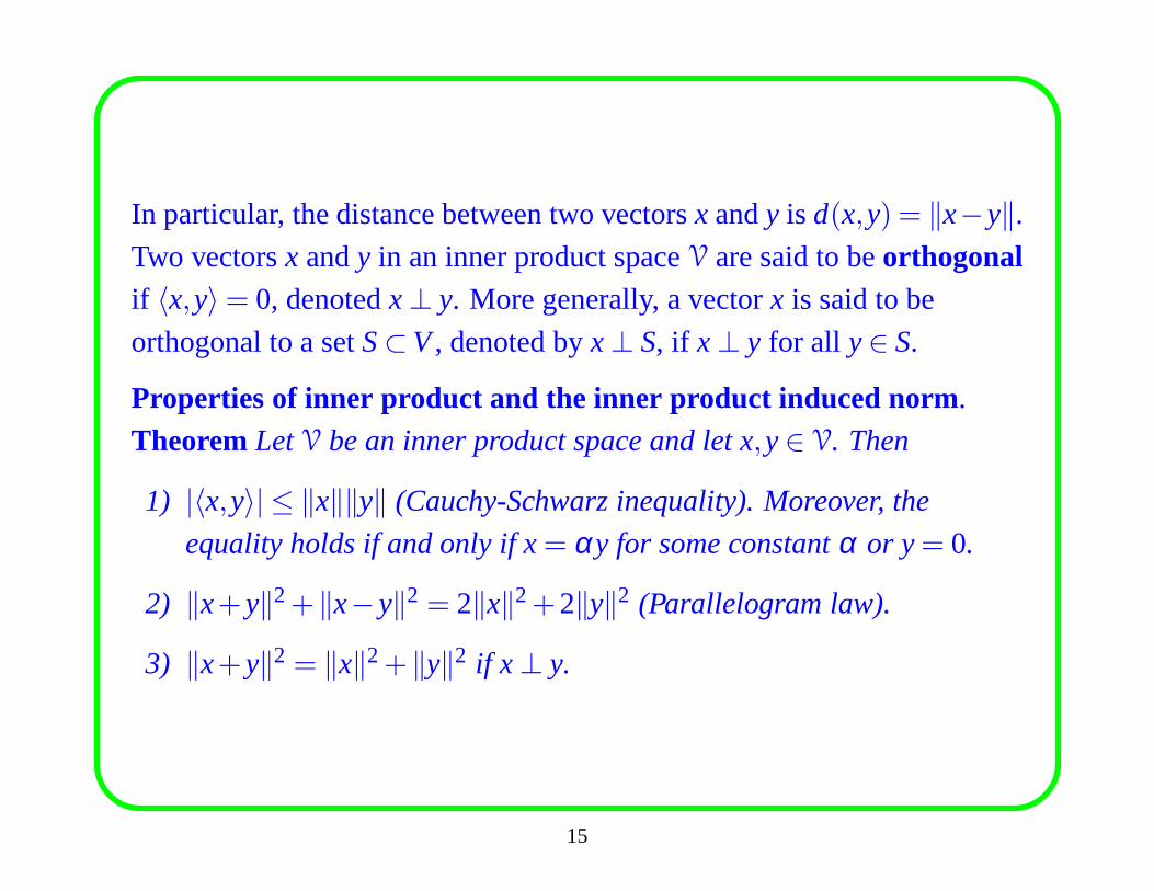
In particular, the distance between two vectorsx andy is d(x,y) = ‖x−y‖.

Two vectorsx andy in an inner product spaceV are said to beorthogonalif 〈x,y〉= 0, denotedx⊥ y. More generally, a vectorx is said to be

orthogonal to a setS⊂V, denoted byx⊥ S, if x⊥ y for all y∈ S.

Properties of inner product and the inner product induced norm .

Theorem LetV be an inner product space and let x,y∈ V. Then

1) |〈x,y〉| ≤ ‖x‖‖y‖ (Cauchy-Schwarz inequality). Moreover, the

equality holds if and only if x= αy for some constantα or y= 0.

2) ‖x+y‖2+‖x−y‖2 = 2‖x‖2+2‖y‖2 (Parallelogram law).

3) ‖x+y‖2 = ‖x‖2+‖y‖2 if x ⊥ y.

15

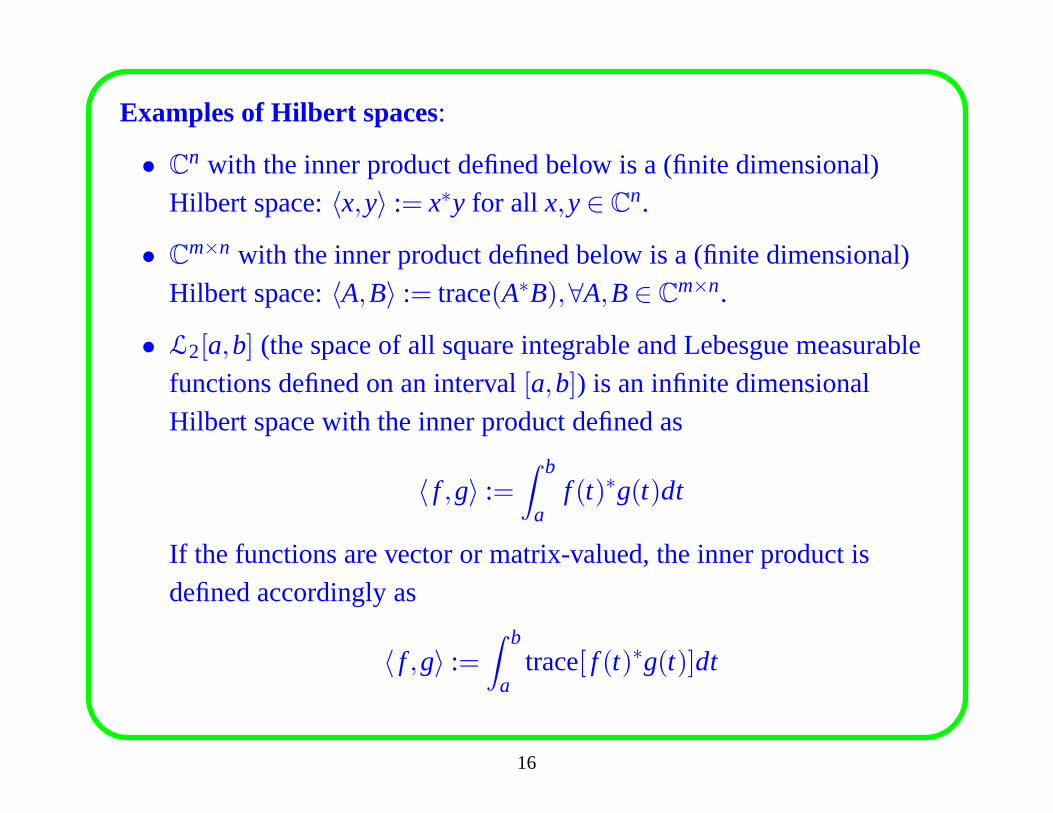
Examples of Hilbert spaces:

• Cn with the inner product defined below is a (finite dimensional)

Hilbert space:〈x,y〉 := x∗y for all x,y∈ Cn.

• Cm×n with the inner product defined below is a (finite dimensional)Hilbert space:〈A,B〉 := trace(A∗B),∀A,B∈ C

m×n.

• L2[a,b] (the space of all square integrable and Lebesgue measurablefunctions defined on an interval[a,b]) is an infinite dimensionalHilbert space with the inner product defined as

〈 f ,g〉 :=∫ b

af (t)∗g(t)dt

If the functions are vector or matrix-valued, the inner product isdefined accordingly as

〈 f ,g〉 :=∫ b

atrace[ f (t)∗g(t)]dt

16

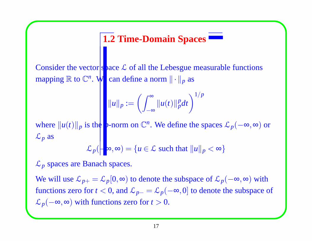
1.2 Time-Domain Spaces

Consider the vector spaceL of all the Lebesgue measurable functions

mappingR toCn. We can define a norm‖ · ‖p as

‖u‖p :=

(∫ ∞

−∞‖u(t)‖p

pdt

)1/p

where‖u(t)‖p is thep-norm onCn. We define the spacesLp(−∞,∞) or

Lp as

Lp(−∞,∞) = {u∈ L such that‖u‖p < ∞}Lp spaces are Banach spaces.

We will useLp+ = Lp[0,∞) to denote the subspace ofLp(−∞,∞) with

functions zero fort < 0, andLp− = Lp(−∞,0] to denote the subspace of

Lp(−∞,∞) with functions zero fort > 0.

17

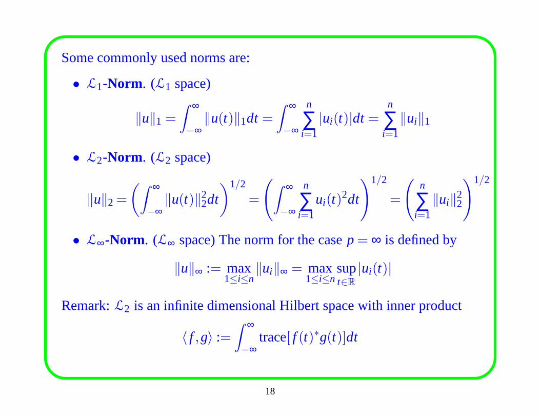
Some commonly used norms are:

• L1-Norm. (L1 space)

‖u‖1 =∫ ∞

−∞‖u(t)‖1dt =

∫ ∞

−∞

n

∑i=1

|ui(t)|dt =n

∑i=1

‖ui‖1

• L2-Norm. (L2 space)

‖u‖2=

(∫ ∞

−∞‖u(t)‖2

2dt

)1/2

=

(∫ ∞

−∞

n

∑i=1

ui(t)2dt

)1/2

=

(n

∑i=1

‖ui‖22

)1/2

• L∞-Norm. (L∞ space) The norm for the casep= ∞ is defined by

‖u‖∞ := max1≤i≤n

‖ui‖∞ = max1≤i≤n

supt∈R

|ui(t)|

Remark:L2 is an infinite dimensional Hilbert space with inner product

〈 f ,g〉 :=∫ ∞

−∞trace[ f (t)∗g(t)]dt

18

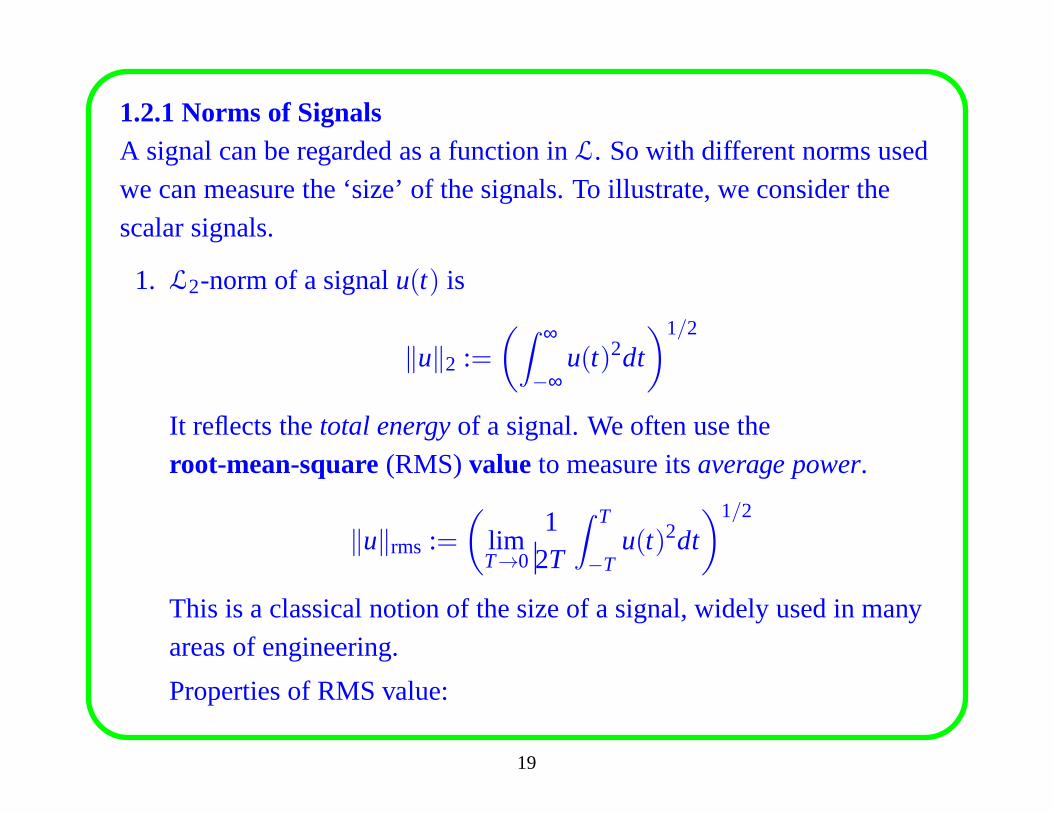
1.2.1 Norms of SignalsA signal can be regarded as a function inL. So with different norms usedwe can measure the ‘size’ of the signals. To illustrate, we consider the

scalar signals.

1. L2-norm of a signalu(t) is

‖u‖2 :=

(∫ ∞

−∞u(t)2dt

)1/2

It reflects thetotal energyof a signal. We often use theroot-mean-square(RMS)value to measure itsaverage power.

‖u‖rms :=

(

limT→0

12T

∫ T

−Tu(t)2dt

)1/2

This is a classical notion of the size of a signal, widely usedin manyareas of engineering.

Properties of RMS value:

19

• RMS is not a norm, since‖u‖rms can be zero whenu is nonzero.

Nevertheless, it is a useful, and often used, measure of a signal’s

size.

• It is known that even if the RMS value of a signal is small, the

signal may occasionally have large peaks, provided the peaks are

not too frequent and do not contain too much energy. In this

sense,‖u‖rms is less affected by large but infrequent values of the

signal.

• The RMS is asteady-statemeasure of a signal; the RMS value of

a signal is not affected by any transient. In particular, a signal with

small RMS value can be very large for some initial time period.

20

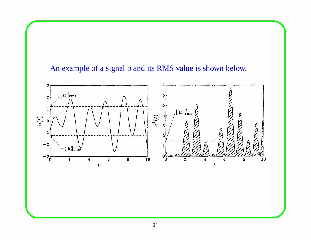
An example of a signalu and its RMS value is shown below.

21

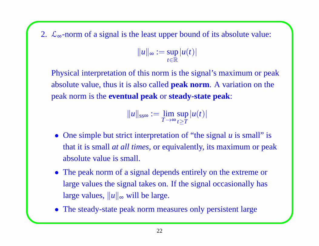
2. L∞-norm of a signal is the least upper bound of its absolute value:

‖u‖∞ := supt∈R

|u(t)|

Physical interpretation of this norm is the signal’s maximum or peakabsolute value, thus it is also calledpeak norm. A variation on thepeak norm is theeventual peakor steady-state peak:

‖u‖ss∞ := limT→∞

supt≥T

|u(t)|

• One simple but strict interpretation of “the signalu is small” isthat it is smallat all times, or equivalently, its maximum or peakabsolute value is small.

• The peak norm of a signal depends entirely on the extreme or

large values the signal takes on. If the signal occasionallyhaslarge values,‖u‖∞ will be large.

• The steady-state peak norm measures only persistent large

22

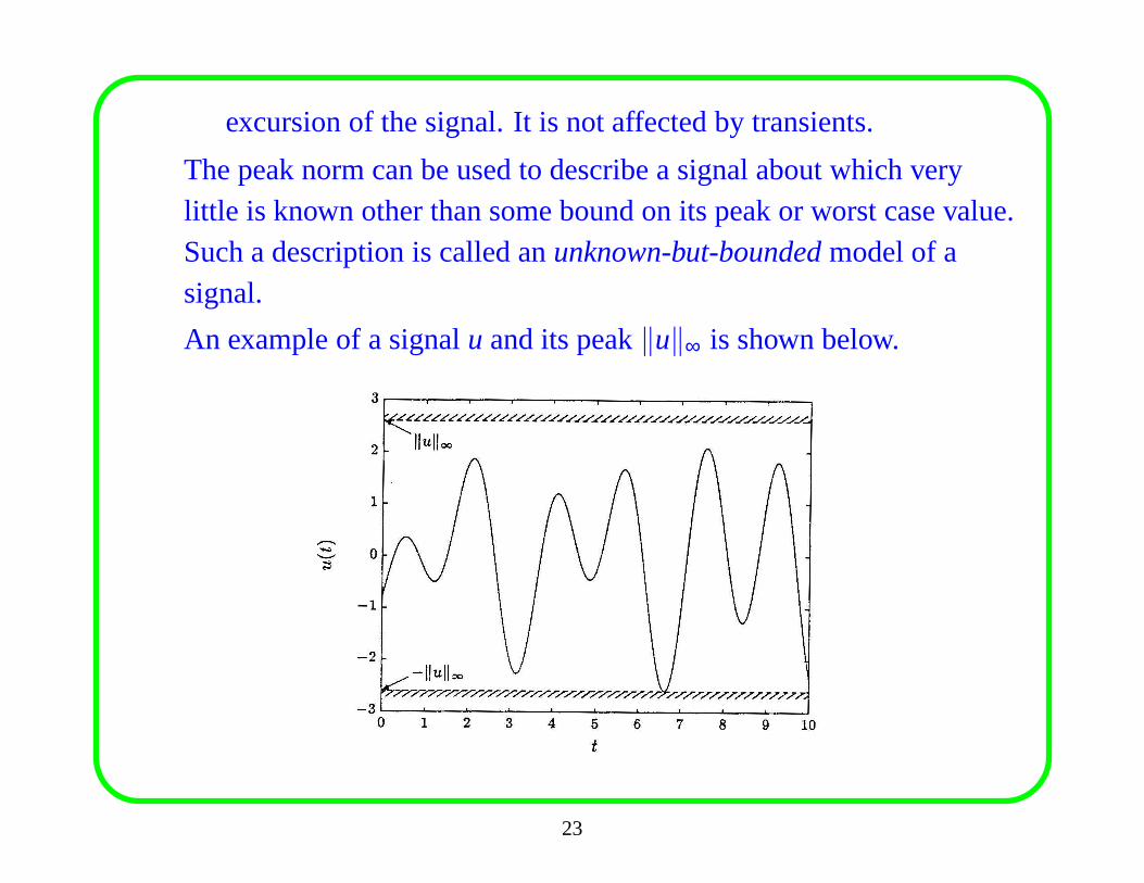
excursion of the signal. It is not affected by transients.

The peak norm can be used to describe a signal about which verylittle is known other than some bound on its peak or worst casevalue.Such a description is called anunknown-but-boundedmodel of asignal.

An example of a signalu and its peak‖u‖∞ is shown below.

23

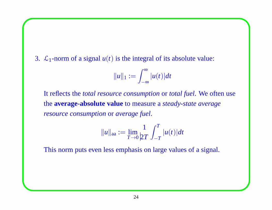
3. L1-norm of a signalu(t) is the integral of its absolute value:

‖u‖1 :=∫ ∞

−∞|u(t)|dt

It reflects thetotal resource consumptionor total fuel. We often use

theaverage-absolute valueto measure asteady-state average

resource consumptionor average fuel.

‖u‖aa := limT→0

12T

∫ T

−T|u(t)|dt

This norm puts even less emphasis on large values of a signal.

24

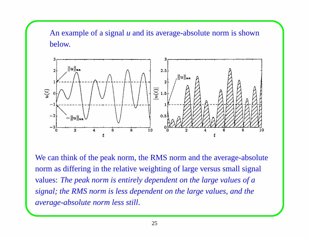
An example of a signalu and its average-absolute norm is shownbelow.

We can think of the peak norm, the RMS norm and the average-absolutenorm as differing in the relative weighting of large versus small signalvalues:The peak norm is entirely dependent on the large values of a

signal; the RMS norm is less dependent on the large values, and the

average-absolute norm less still.

25

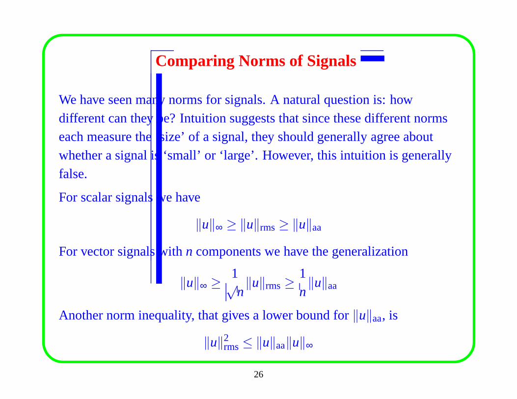
Comparing Norms of Signals

We have seen many norms for signals. A natural question is: howdifferent can they be? Intuition suggests that since these different normseach measure the ‘size’ of a signal, they should generally agree aboutwhether a signal is ‘small’ or ‘large’. However, this intuition is generallyfalse.

For scalar signals we have

‖u‖∞ ≥ ‖u‖rms≥ ‖u‖aa

For vector signals withn components we have the generalization

‖u‖∞ ≥ 1√n‖u‖rms≥

1n‖u‖aa

Another norm inequality, that gives a lower bound for‖u‖aa, is

‖u‖2rms≤ ‖u‖aa‖u‖∞

26

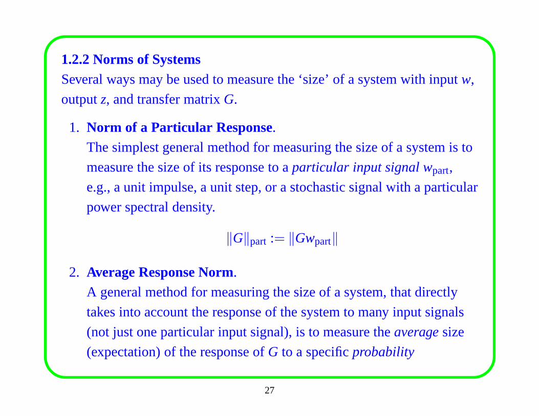
1.2.2 Norms of SystemsSeveral ways may be used to measure the ‘size’ of a system withinputw,

outputz, and transfer matrixG.

1. Norm of a Particular Response.The simplest general method for measuring the size of a system is to

measure the size of its response to aparticular input signal wpart,

e.g., a unit impulse, a unit step, or a stochastic signal witha particular

power spectral density.

‖G‖part := ‖Gwpart‖

2. Average Response Norm.A general method for measuring the size of a system, that directly

takes into account the response of the system to many input signals

(not just one particular input signal), is to measure theaveragesize

(expectation) of the response ofG to a specificprobability

27

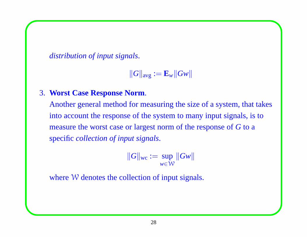
distribution of input signals.

‖G‖avg := Ew‖Gw‖

3. Worst Case Response Norm.Another general method for measuring the size of a system, that takes

into account the response of the system to many input signals, is to

measure the worst case or largest norm of the response ofG to a

specificcollection of input signals.

‖G‖wc := supw∈W

‖Gw‖

whereW denotes the collection of input signals.

28

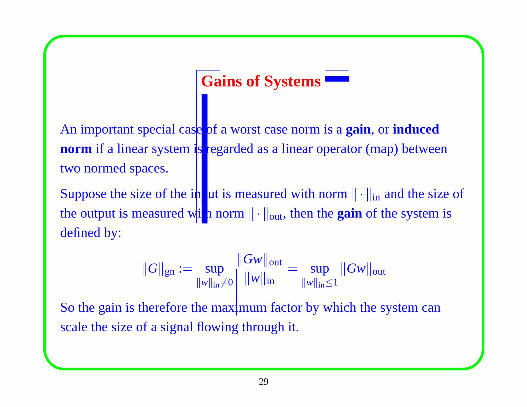
Gains of Systems

An important special case of a worst case norm is again, or inducednorm if a linear system is regarded as a linear operator (map) between

two normed spaces.

Suppose the size of the input is measured with norm‖ · ‖in and the size of

the output is measured with norm‖ · ‖out, then thegain of the system is

defined by:

‖G‖gn := sup‖w‖in 6=0

‖Gw‖out

‖w‖in= sup

‖w‖in≤1‖Gw‖out

So the gain is therefore the maximum factor by which the system can

scale the size of a signal flowing through it.

29

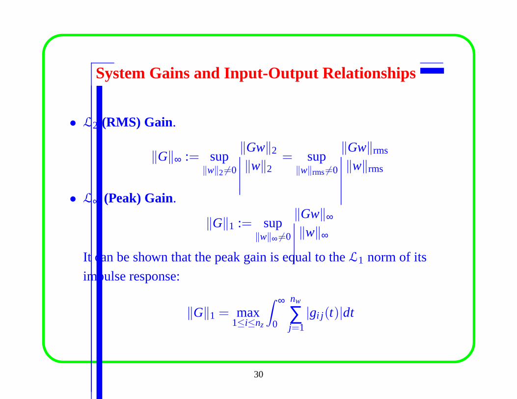
System Gains and Input-Output Relationships

• L2 (RMS) Gain.

‖G‖∞ := sup‖w‖2 6=0

‖Gw‖2

‖w‖2= sup

‖w‖rms6=0

‖Gw‖rms

‖w‖rms

• L∞ (Peak) Gain.

‖G‖1 := sup‖w‖∞ 6=0

‖Gw‖∞

‖w‖∞

It can be shown that the peak gain is equal to theL1 norm of its

impulse response:

‖G‖1 = max1≤i≤nz

∫ ∞

0

nw

∑j=1

|gi j (t)|dt

30

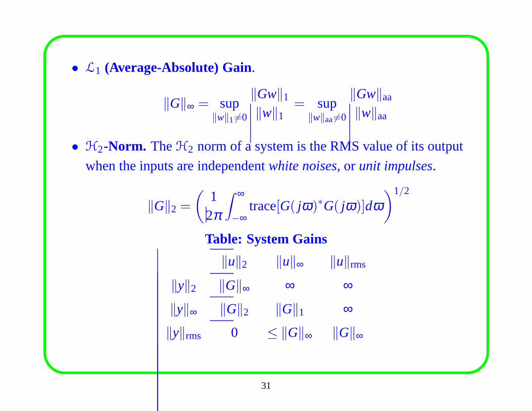
• L1 (Average-Absolute) Gain.

‖G‖∞ = sup‖w‖1 6=0

‖Gw‖1

‖w‖1= sup

‖w‖aa6=0

‖Gw‖aa

‖w‖aa

• H2-Norm. TheH2 norm of a system is the RMS value of its output

when the inputs are independentwhite noises, or unit impulses.

‖G‖2 =

(1

2π

∫ ∞

−∞trace[G( jω)∗G( jω)]dω

)1/2

Table: System Gains

‖u‖2 ‖u‖∞ ‖u‖rms

‖y‖2 ‖G‖∞ ∞ ∞

‖y‖∞ ‖G‖2 ‖G‖1 ∞

‖y‖rms 0 ≤ ‖G‖∞ ‖G‖∞

31

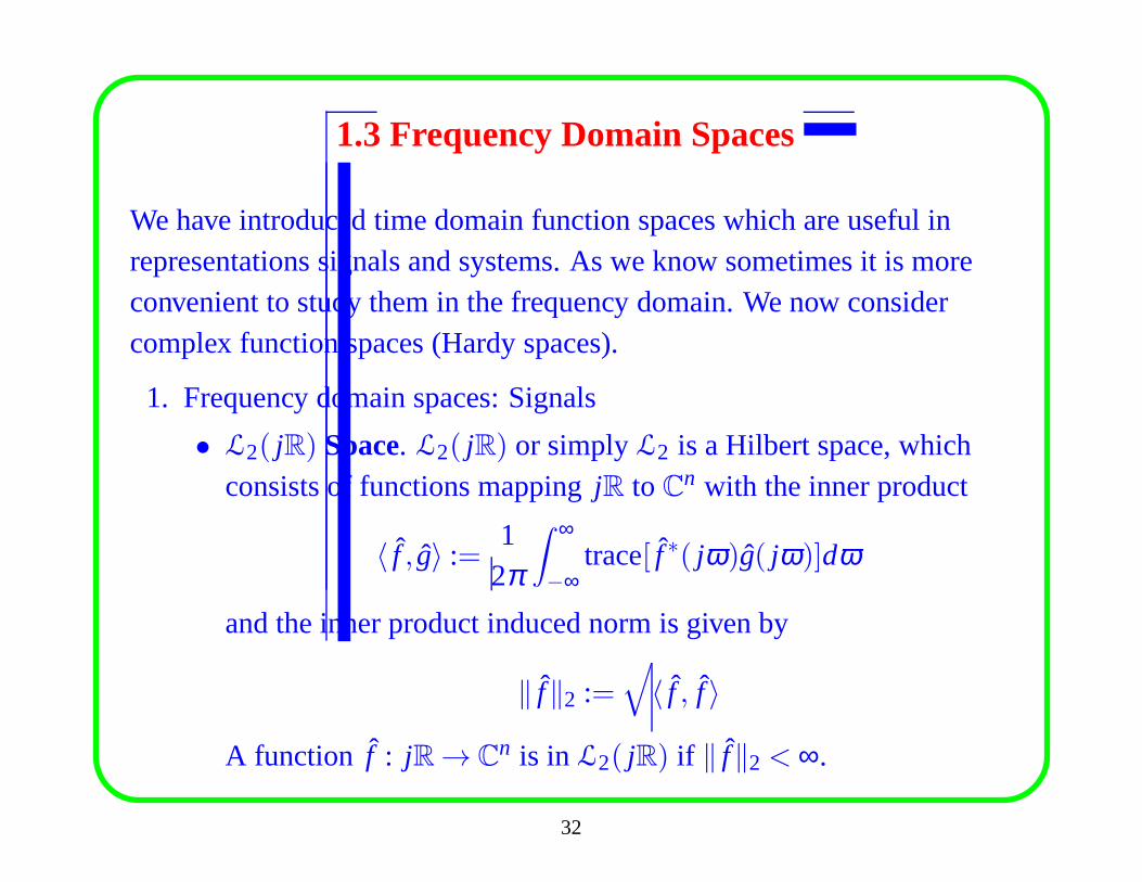
1.3 Frequency Domain Spaces

We have introduced time domain function spaces which are useful inrepresentations signals and systems. As we know sometimes it is moreconvenient to study them in the frequency domain. We now considercomplex function spaces (Hardy spaces).

1. Frequency domain spaces: Signals

• L2( jR) Space. L2( jR) or simplyL2 is a Hilbert space, whichconsists of functions mappingjR toC

n with the inner product

〈 f , g〉 :=1

2π

∫ ∞

−∞trace[ f ∗( jω)g( jω)]dω

and the inner product induced norm is given by

‖ f‖2 :=√

〈 f , f 〉

A function f : jR→ Cn is inL2( jR) if ‖ f‖2 < ∞.

32

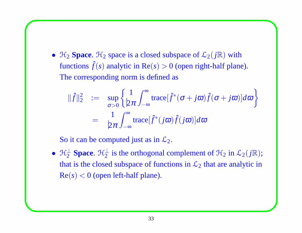
• H2 Space. H2 space is a closed subspace ofL2( jR) with

functions f (s) analytic in Re(s)> 0 (open right-half plane).

The corresponding norm is defined as

‖ f‖22 := sup

σ>0

{1

2π

∫ ∞

−∞trace[ f ∗(σ + jω) f (σ + jω)]dω

}

=1

2π

∫ ∞

−∞trace[ f ∗( jω) f ( jω)]dω

So it can be computed just as inL2.

• H⊥2 Space. H⊥

2 is the orthogonal complement ofH2 in L2( jR);

that is the closed subspace of functions inL2 that are analytic in

Re(s)< 0 (open left-half plane).

33

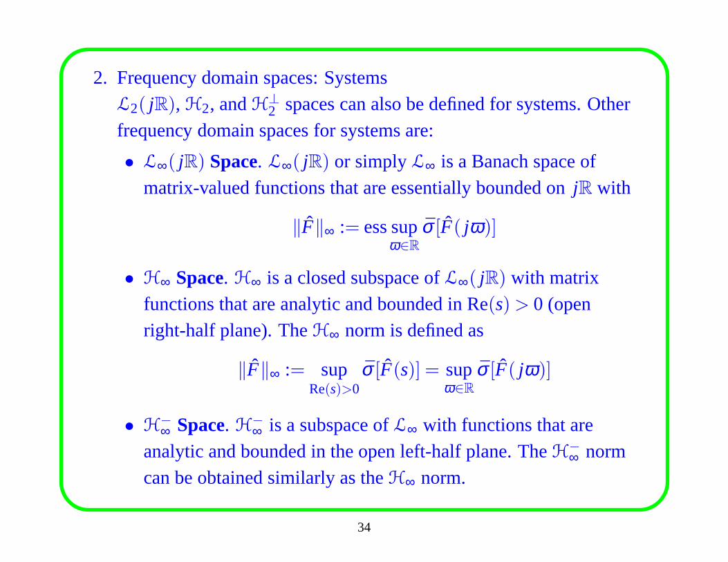
2. Frequency domain spaces: SystemsL2( jR), H2, andH⊥

2 spaces can also be defined for systems. Otherfrequency domain spaces for systems are:

• L∞( jR) Space. L∞( jR) or simplyL∞ is a Banach space ofmatrix-valued functions that are essentially bounded onjR with

‖F‖∞ := ess supω∈R

σ [F( jω)]

• H∞ Space. H∞ is a closed subspace ofL∞( jR) with matrixfunctions that are analytic and bounded in Re(s)> 0 (openright-half plane). TheH∞ norm is defined as

‖F‖∞ := supRe(s)>0

σ [F(s)] = supω∈R

σ [F( jω)]

• H−∞ Space. H−

∞ is a subspace ofL∞ with functions that areanalytic and bounded in the open left-half plane. TheH−

∞ normcan be obtained similarly as theH∞ norm.

34

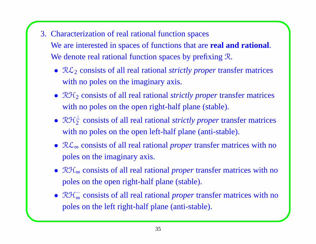
3. Characterization of real rational function spacesWe are interested in spaces of functions that arereal and rational.We denote real rational function spaces by prefixingR.

• RL2 consists of all real rationalstrictly propertransfer matriceswith no poles on the imaginary axis.

• RH2 consists of all real rationalstrictly propertransfer matriceswith no poles on the open right-half plane (stable).

• RH⊥2 consists of all real rationalstrictly propertransfer matrices

with no poles on the open left-half plane (anti-stable).

• RL∞ consists of all real rationalproper transfer matrices with nopoles on the imaginary axis.

• RH∞ consists of all real rationalproper transfer matrices with nopoles on the open right-half plane (stable).

• RH−∞ consists of all real rationalproper transfer matrices with no

poles on the left right-half plane (anti-stable).

35

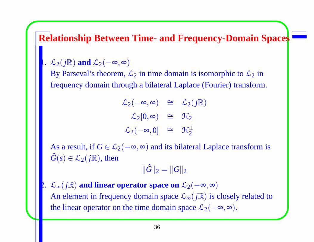
Relationship Between Time- and Frequency-Domain Spaces

1. L2( jR) and L2(−∞,∞)

By Parseval’s theorem,L2 in time domain is isomorphic toL2 infrequency domain through a bilateral Laplace (Fourier) transform.

L2(−∞,∞) ∼= L2( jR)

L2[0,∞) ∼= H2

L2(−∞,0] ∼= H⊥2

As a result, ifG∈ L2(−∞,∞) and its bilateral Laplace transform isG(s) ∈ L2( jR), then

‖G‖2 = ‖G‖2

2. L∞( jR) and linear operator space onL2(−∞,∞)

An element in frequency domain spaceL∞( jR) is closely related tothe linear operator on the time domain spaceL2(−∞,∞).

36

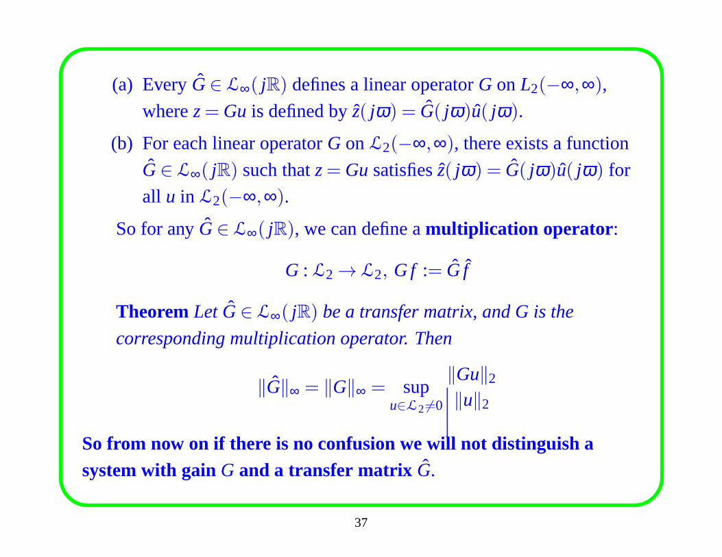
(a) EveryG∈ L∞( jR) defines a linear operatorG on L2(−∞,∞),

wherez= Gu is defined by ˆz( jω) = G( jω)u( jω).

(b) For each linear operatorG onL2(−∞,∞), there exists a function

G∈ L∞( jR) such thatz= Gu satisfies ˆz( jω) = G( jω)u( jω) for

all u in L2(−∞,∞).

So for anyG∈ L∞( jR), we can define amultiplication operator :

G : L2 → L2, G f := G f

Theorem Let G∈ L∞( jR) be a transfer matrix, and G is the

corresponding multiplication operator. Then

‖G‖∞ = ‖G‖∞ = supu∈L2 6=0

‖Gu‖2

‖u‖2

So from now on if there is no confusion we will not distinguishasystem with gainG and a transfer matrix G.

37

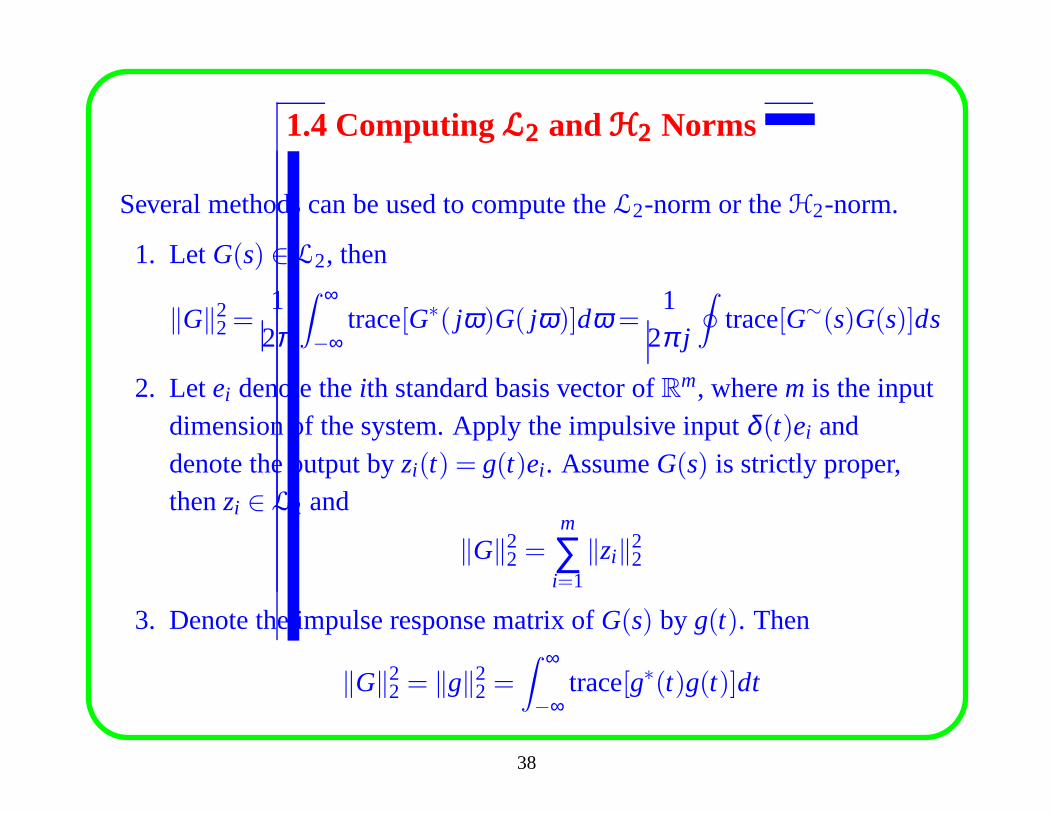
1.4 ComputingL2L2L2 andH2H2H2 Norms

Several methods can be used to compute theL2-norm or theH2-norm.

1. LetG(s) ∈ L2, then

‖G‖22=

12π

∫ ∞

−∞trace[G∗( jω)G( jω)]dω =

12π j

∮

trace[G∼(s)G(s)]ds

2. Letei denote theith standard basis vector ofRm, wherem is the inputdimension of the system. Apply the impulsive inputδ (t)ei anddenote the output byzi(t) = g(t)ei . AssumeG(s) is strictly proper,thenzi ∈ L2 and

‖G‖22 =

m

∑i=1

‖zi‖22

3. Denote the impulse response matrix ofG(s) by g(t). Then

‖G‖22 = ‖g‖2

2 =∫ ∞

−∞trace[g∗(t)g(t)]dt

38

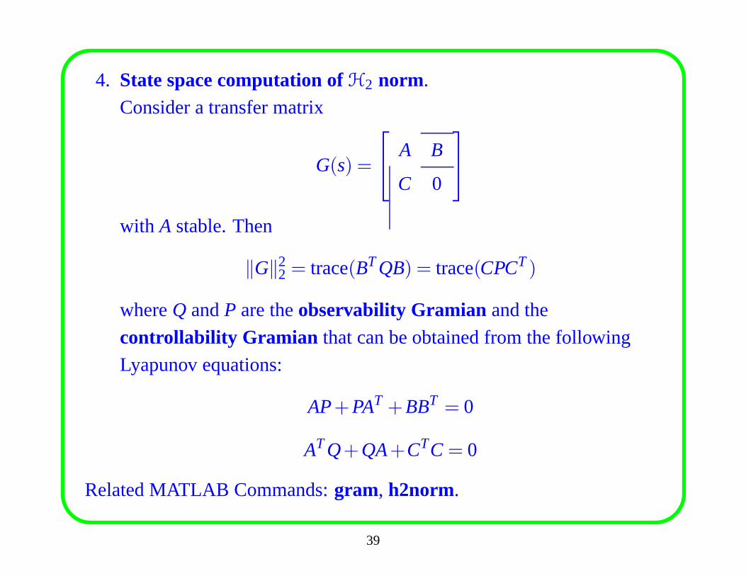
4. State space computation ofH2 norm.

Consider a transfer matrix

G(s) =

A B

C 0

with A stable. Then

‖G‖22 = trace(BTQB) = trace(CPCT)

whereQ andP are theobservability Gramian and the

controllability Gramian that can be obtained from the following

Lyapunov equations:

AP+PAT +BBT = 0

ATQ+QA+CTC = 0

Related MATLAB Commands:gram, h2norm.

39

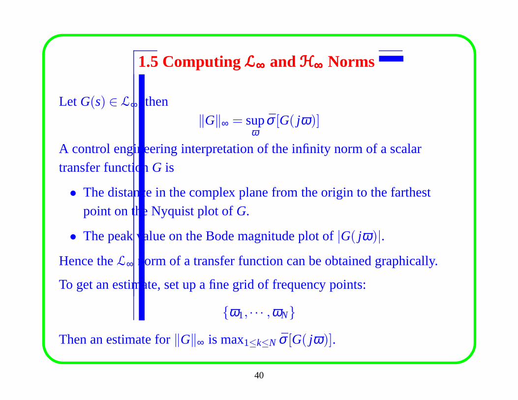
1.5 ComputingL∞L∞L∞ andH∞H∞H∞ Norms

Let G(s) ∈ L∞, then‖G‖∞ = sup

ωσ [G( jω)]

A control engineering interpretation of the infinity norm ofa scalartransfer functionG is

• The distance in the complex plane from the origin to the farthestpoint on the Nyquist plot ofG.

• The peak value on the Bode magnitude plot of|G( jω)|.Hence theL∞ norm of a transfer function can be obtained graphically.

To get an estimate, set up a fine grid of frequency points:

{ω1, · · · ,ωN}

Then an estimate for‖G‖∞ is max1≤k≤N σ [G( jω)].

40

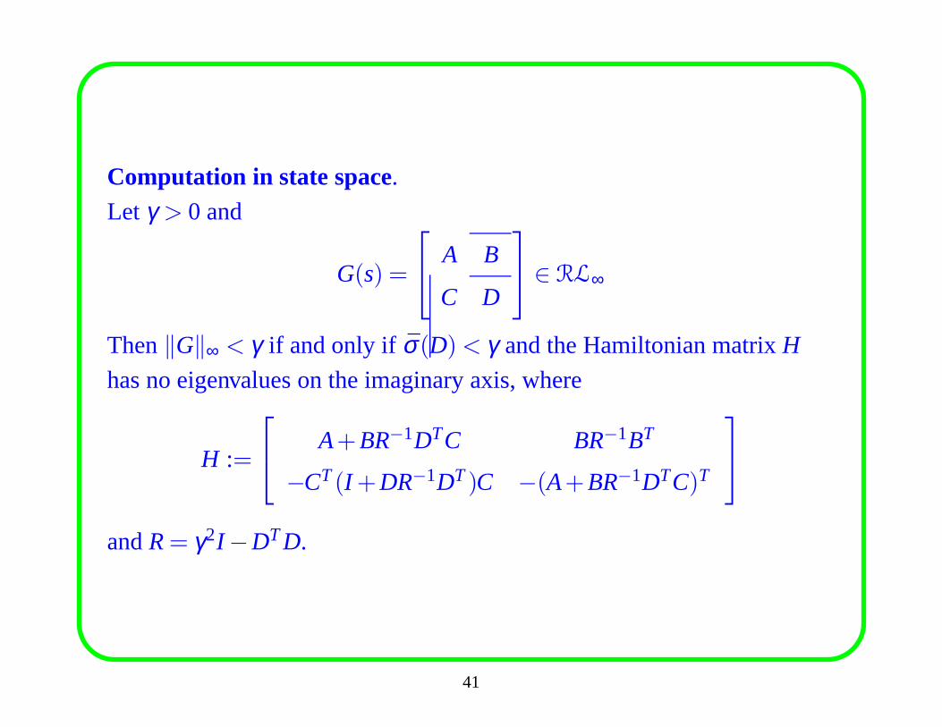
Computation in state space.Let γ > 0 and

G(s) =

A B

C D

∈ RL∞

Then‖G‖∞ < γ if and only if σ(D)< γ and the Hamiltonian matrixH

has no eigenvalues on the imaginary axis, where

H :=

A+BR−1DTC BR−1BT

−CT(I +DR−1DT)C −(A+BR−1DTC)T

andR= γ2I −DTD.

41

Bisection AlgorithmWe can use the following bisection algorithm to computeRL∞ norm:

(a) Select an upper boundγu and a lower boundγl such that

γl ≤ ‖G‖∞ ≤ γu.

(b) If (γu− γl )/γl ≤ specified level, stop;‖G‖∞ ≈ (γu+ γl )/2. Otherwise

go to the next step.

(c) Setγ = (γu+ γl )/2;

(d) Test if‖G‖∞ < γ by calculating the eigenvalues ofH for the givenγ.

(e) If H has an eigenvalue onjR, setγl = γ; otherwise setγu = γ; go

back to step (b).

The above algorithm applies toH∞ norm computation as well.

Related MATLAB Commands:sigma, hinfnorm .

42

Chapter 2. Uncertainty and Robustness

In this chapter we will describe various types of uncertainties that can

arise in physical systems, and obtain robust stability tests for systems

under various model uncertainty assumptions. Outline of this chapter:

• Model uncertainty description

• Small gain theorem and smallµ theorem

• Robust stability under unstructured and structured uncertainties

• Linear fractional transformation (LFT) and Main Loop Theorem

43

Model Uncertainty

Modeling of plant uncertainty can be done in two methods:

• Unstructured uncertainty. Unstructured uncertainty is the uncertainty

about which no information is available about its effects ona process,

except that an upper bound on its ‘size’ or magnitude as a function of

frequency can be estimated.

• Structured uncertainty. Structured uncertainty is the uncertainty

about which ‘structural’ information is available, which will typically

restrict to a section of a process model. It is also calledparameter

uncertainty.

44

2.1 Unstructured Uncertainty

Several methods can be used to model unstructured uncertainty.

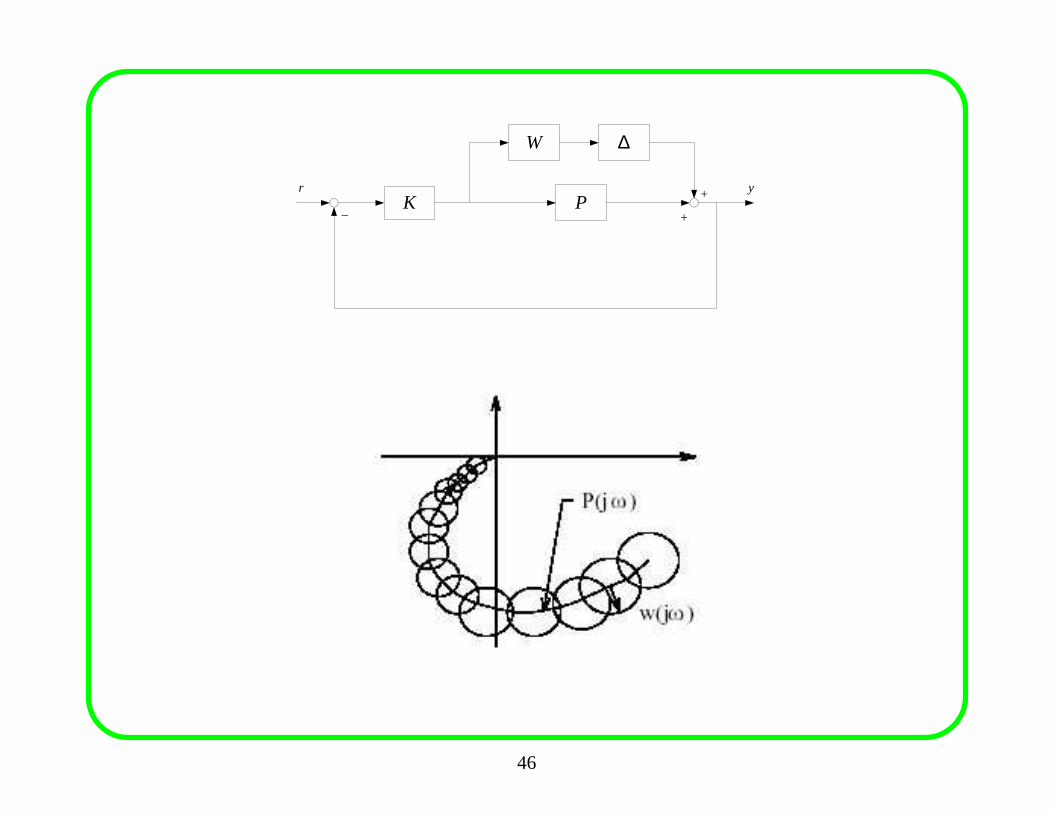
1. Additive UncertaintySuppose that the nominal plant transfer matrix isP and consider

perturbed plant transfer matrices of the form

P∆ = P+∆W

HereW is a fixed stable transfer matrix, the weight, and∆ is a

variable stable transfer matrix satisfying

‖∆‖∞ ≤ 1

Furthermore, it is assumed that no unstable poles ofP are canceled in

forming P∆. Such a perturbation∆ is said to be allowable.

45

K P

W

r

_

y

∆

+

+

46

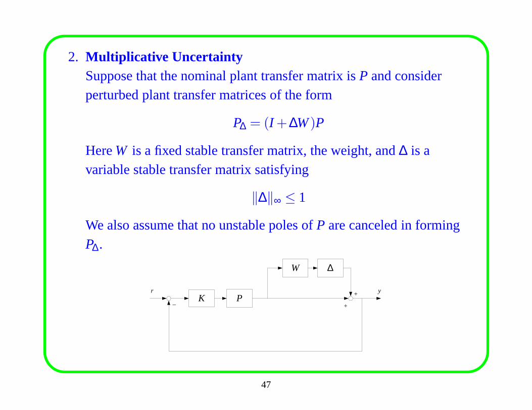
2. Multiplicative UncertaintySuppose that the nominal plant transfer matrix isP and considerperturbed plant transfer matrices of the form

P∆ = (I +∆W)P

HereW is a fixed stable transfer matrix, the weight, and∆ is avariable stable transfer matrix satisfying

‖∆‖∞ ≤ 1

We also assume that no unstable poles ofP are canceled in formingP∆.

K P

W

r

_

y

∆

+

+

47

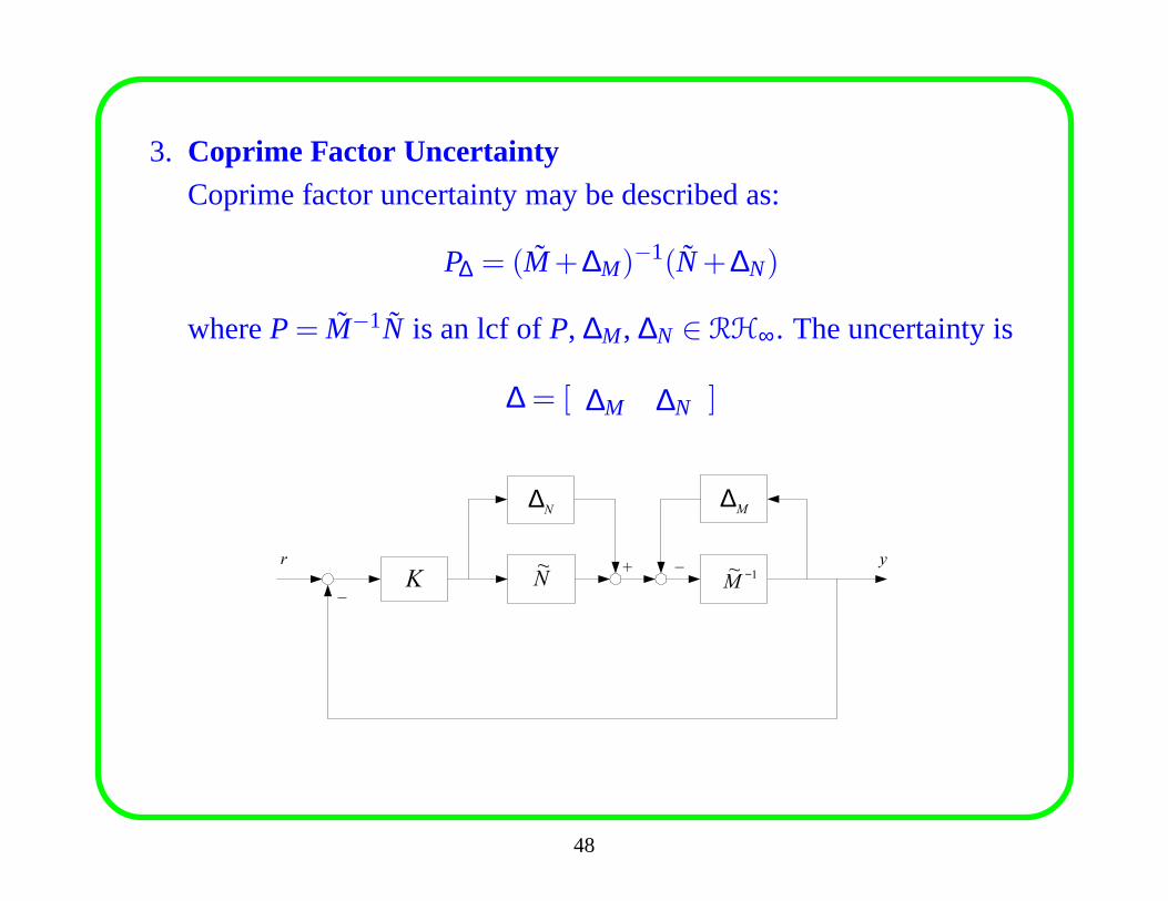
3. Coprime Factor UncertaintyCoprime factor uncertainty may be described as:

P∆ = (M+∆M)−1(N+∆N)

whereP= M−1N is an lcf ofP, ∆M, ∆N ∈ RH∞. The uncertainty is

∆ = [ ∆M ∆N ]

Kr

_

y

∆M

+_

∆N

N~

1~ −M

48

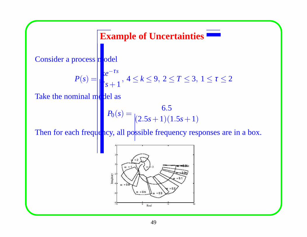
Example of Uncertainties

Consider a process model

P(s) =ke−τs

Ts+1, 4≤ k≤ 9, 2≤ T ≤ 3, 1≤ τ ≤ 2

Take the nominal model as

P0(s) =6.5

(2.5s+1)(1.5s+1)

Then for each frequency, all possible frequency responses are in a box.

49

The additive perturbation is

∆a( jω) = P( jω)−P0( jω)

A weight such that|∆a( jω)| ≤ |Wa( jω)| can be chosen as

Wa(s) =0.0376(s+116.4808)(s+7.4514)(s+0.2674)

(s+1.2436)(s+0.5575)(s+4.9508)

50

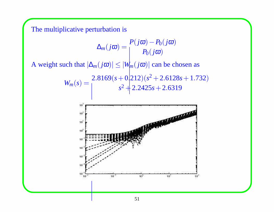
The multiplicative perturbation is

∆m( jω) =P( jω)−P0( jω)

P0( jω)

A weight such that|∆m( jω)| ≤ |Wm( jω)| can be chosen as

Wm(s) =2.8169(s+0.212)(s2+2.6128s+1.732)

s2+2.2425s+2.6319

51

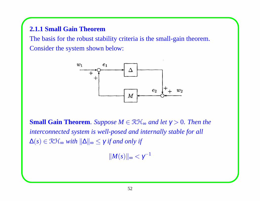
2.1.1 Small Gain TheoremThe basis for the robust stability criteria is the small-gain theorem.

Consider the system shown below:

Small Gain Theorem. Suppose M∈ RH∞ and letγ > 0. Then the

interconnected system is well-posed and internally stablefor all

∆(s) ∈ RH∞ with ‖∆‖∞ ≤ γ if and only if

‖M(s)‖∞ < γ−1

52

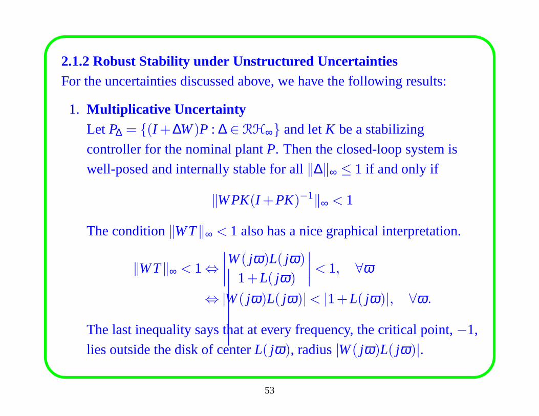
2.1.2 Robust Stability under Unstructured UncertaintiesFor the uncertainties discussed above, we have the following results:

1. Multiplicative UncertaintyLet P∆ = {(I +∆W)P : ∆ ∈ RH∞} and letK be a stabilizing

controller for the nominal plantP. Then the closed-loop system is

well-posed and internally stable for all‖∆‖∞ ≤ 1 if and only if

‖WPK(I +PK)−1‖∞ < 1

The condition‖WT‖∞ < 1 also has a nice graphical interpretation.

‖WT‖∞ < 1⇔∣∣∣∣

W( jω)L( jω)

1+L( jω)

∣∣∣∣< 1, ∀ω

⇔ |W( jω)L( jω)|< |1+L( jω)|, ∀ω.

The last inequality says that at every frequency, the critical point,−1,

lies outside the disk of centerL( jω), radius|W( jω)L( jω)|.

53

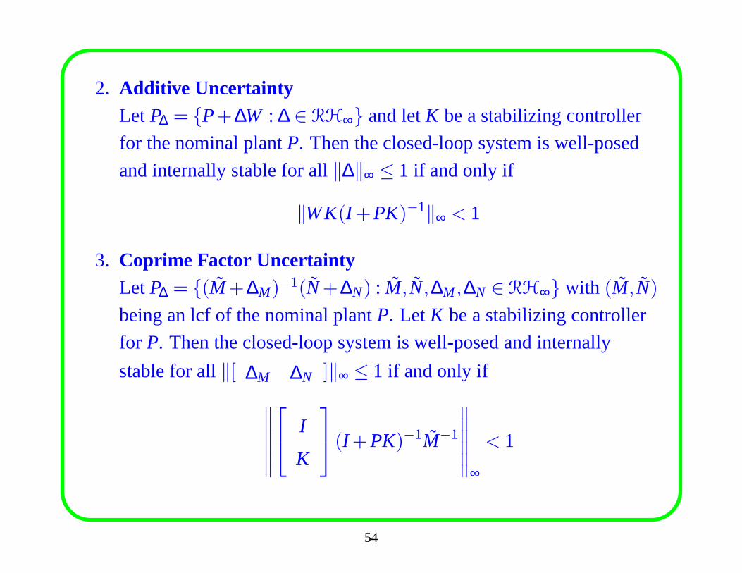
2. Additive UncertaintyLet P∆ = {P+∆W : ∆ ∈ RH∞} and letK be a stabilizing controller

for the nominal plantP. Then the closed-loop system is well-posed

and internally stable for all‖∆‖∞ ≤ 1 if and only if

‖WK(I +PK)−1‖∞ < 1

3. Coprime Factor UncertaintyLet P∆ = {(M+∆M)−1(N+∆N) : M, N,∆M,∆N ∈RH∞} with (M, N)

being an lcf of the nominal plantP. Let K be a stabilizing controller

for P. Then the closed-loop system is well-posed and internally

stable for all‖[ ∆M ∆N ]‖∞ ≤ 1 if and only if

∥∥∥∥∥∥

I

K

(I +PK)−1M−1

∥∥∥∥∥∥

∞

< 1

54

2.2 Structured Uncertainty

It is easy to see that the maximum singular value (H∞-norm) is useful in

analyzing the unstructured uncertainty. To analyze the structured

uncertainty, we need the concept of structured singular value.

The definition of the structured singular value, which is also calledµ,

depends on the underlying block structure of the uncertainty set∆∆∆.

Defining the structure involves specifying three things:

• The type of each block.repeated scalaror full block.

• The total number of blocks. The number ofrepeated scalarblocks is

denoted byS, and the number offull blocks is denoted byF .

• The dimension of each block. To bookkeep the dimensions, we

introduce positive integersc1, · · · ,cS andm1, · · · ,mF . Thei’th

repeated scalar block isci ×ci , and thek’th full block is mk×mk.

55

We define the block structure∆∆∆ ⊂ Cn×n as

∆∆∆ = {diag[δ1Ic1, · · · ,δSIcS,∆1, · · · ,∆F ] : δi ∈ C,∆k ∈ Cmk×mk}

For consistency among all dimensions, we must have

S

∑i=1

ci +F

∑k=1

mk = n

Structured Singular Value (SSV)

Given a matrixM ∈ Cn×n and the underlying structure∆∆∆, µ∆∆∆(M) is

defined as

µ∆∆∆(M) :=1

min{σ(∆) : ∆ ∈∆∆∆,det(I −M∆) = 0}

unless no∆ ∈∆∆∆ makesI −M∆ singular, in which caseµ∆∆∆(M) := 0.

56

For a transfer matrixM(s), define the set of all block diagonal and stablerational transfer functions that have block structures as∆∆∆:

M(∆∆∆) := {∆(·) ∈ RH∞ : ∆(s) ∈∆∆∆ for all s∈ C such that Res≥ 0}

then the structured singular value ofM(s) can be computed pointwise as

‖M(s)‖µ = µ∆∆∆(M(s)) = supω∈R∪{∞}

µ∆∆∆(M( jω))

The functionµ : Cn×n → R is not a norm, since it does not satisfy thetriangle inequality. However, for simplicity, we still use‖ · ‖µ .Properties ofµµµ :

• If ∆∆∆ = {δ I : δ ∈ C} (complex repeated scalar block,S= 1,F = 0),thenµ∆∆∆(M) = ρ(M).

• If ∆∆∆ = Cn×n (full block, S= 0,F = 1), thenµ∆∆∆(M) = σ(M).

• ρ(M)≤ µ∆∆∆(M)≤ σ(M), µ∆∆∆(M) = max∆∈∆∆∆,σ(∆)≤1 ρ(M∆).

Related MATLAB Command:mu(M,blk)

57

2.2.1 Upper and Lower Bounds ofµµµThe structured singular value lies between the spectral radius and the

maximum singular value ofM. However, the two bounds can be

arbitrarily far. To get a tight upper and lower bounds, we consider

transformations onM that do not affectµ∆∆∆(M), but do affectρ andσ .

To do this, define the following two subsets ofCn×n:

U := {U ∈∆∆∆ : UU∗ = In}D := {D ∈ Cn×n : detD 6= 0,D∆ = ∆D,∀∆ ∈∆∆∆}

= {D1, . . . ,DS,d1Im1, . . . ,dF ImF : Di ∈ Cci×ci ,d j ∈ C}

Note that for any∆ ∈∆∆∆, U ∈ U, andD ∈D, we have

U∗ ∈ U,U∆ ∈∆∆∆,∆U ∈∆∆∆,σ(U∆) = σ(∆U) = σ(∆)

D∆ = ∆D

58

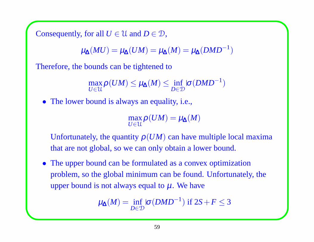
Consequently, for allU ∈ U andD ∈D,

µ∆∆∆(MU) = µ∆∆∆(UM) = µ∆∆∆(M) = µ∆∆∆(DMD−1)

Therefore, the bounds can be tightened to

maxU∈U

ρ(UM)≤ µ∆∆∆(M)≤ infD∈D

σ(DMD−1)

• The lower bound is always an equality, i.e.,

maxU∈U

ρ(UM) = µ∆∆∆(M)

Unfortunately, the quantityρ(UM) can have multiple local maximathat are not global, so we can only obtain a lower bound.

• The upper bound can be formulated as a convex optimizationproblem, so the global minimum can be found. Unfortunately,theupper bound is not always equal toµ. We have

µ∆∆∆(M) = infD∈D

σ(DMD−1) if 2S+F ≤ 3

59

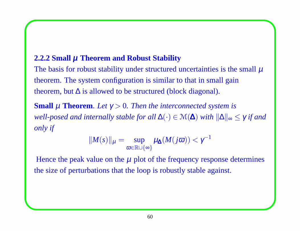
2.2.2 Smallµµµ Theorem and Robust StabilityThe basis for robust stability under structured uncertainties is the smallµtheorem. The system configuration is similar to that in smallgain

theorem, but∆ is allowed to be structured (block diagonal).

Small µ Theorem. Let γ > 0. Then the interconnected system is

well-posed and internally stable for all∆(·) ∈M(∆∆∆) with ‖∆‖∞ ≤ γ if and

only if

‖M(s)‖µ = supω∈R∪{∞}

µ∆∆∆(M( jω))< γ−1

Hence the peak value on theµ plot of the frequency response determines

the size of perturbations that the loop is robustly stable against.

60

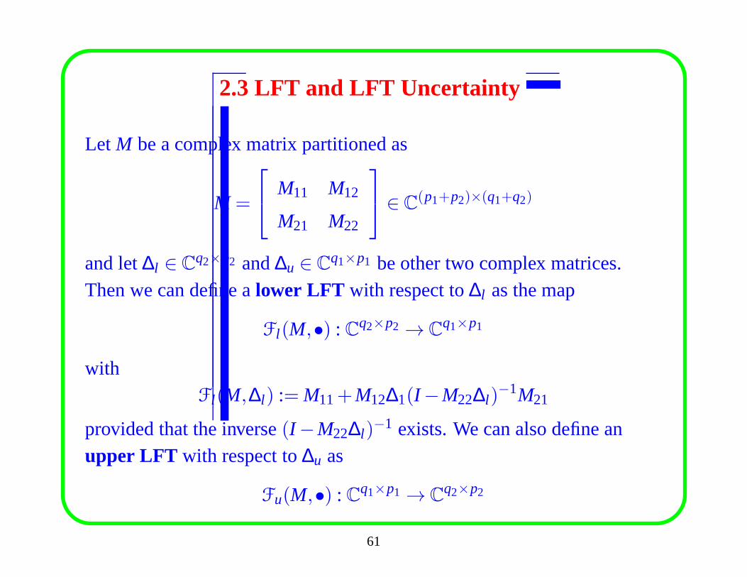
2.3 LFT and LFT Uncertainty

Let M be a complex matrix partitioned as

M =

M11 M12

M21 M22

∈ C(p1+p2)×(q1+q2)

and let∆l ∈ Cq2×p2 and∆u ∈ Cq1×p1 be other two complex matrices.Then we can define alower LFT with respect to∆l as the map

Fl (M,•) : Cq2×p2 → Cq1×p1

withFl (M,∆l ) := M11+M12∆1(I −M22∆l )

−1M21

provided that the inverse(I −M22∆l )−1 exists. We can also define an

upper LFT with respect to∆u as

Fu(M,•) : Cq1×p1 → Cq2×p2

61

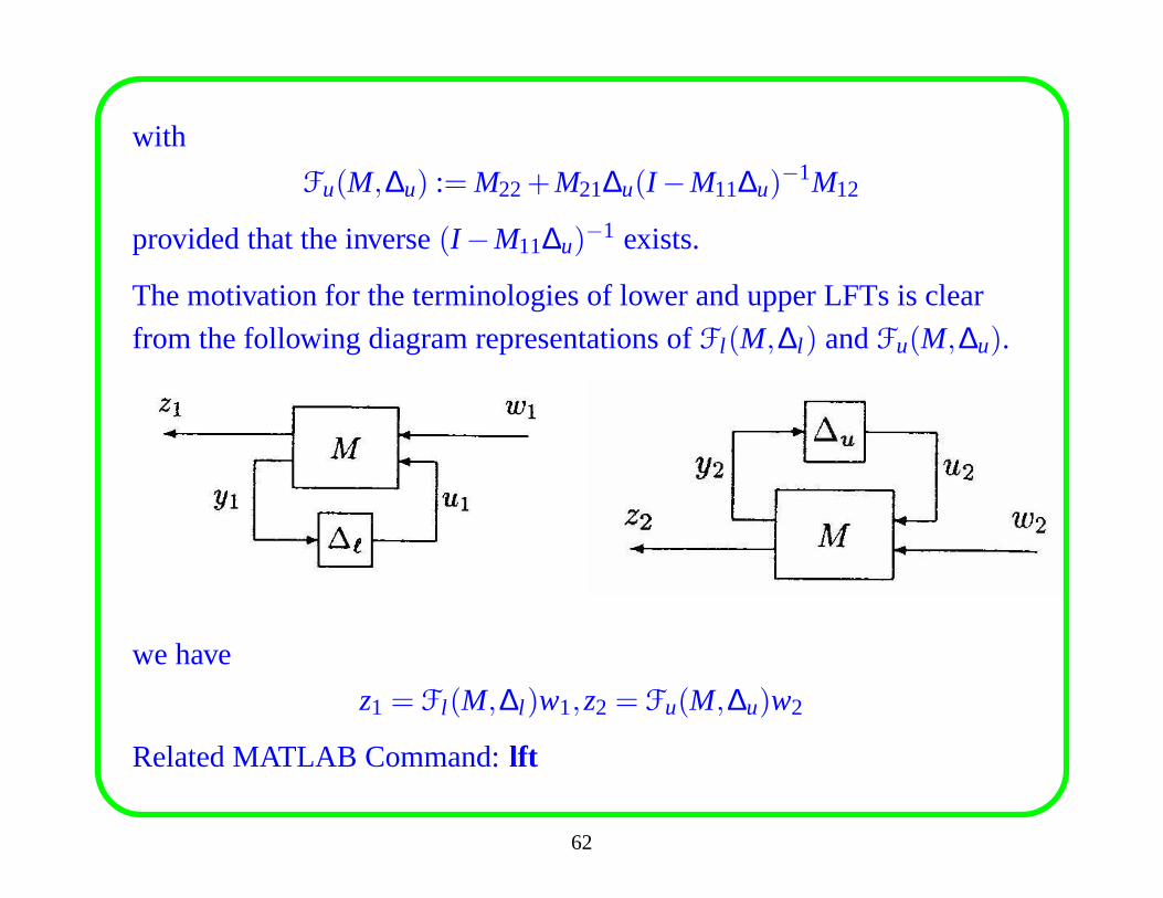
with

Fu(M,∆u) := M22+M21∆u(I −M11∆u)−1M12

provided that the inverse(I −M11∆u)−1 exists.

The motivation for the terminologies of lower and upper LFTsis clear

from the following diagram representations ofFl (M,∆l ) andFu(M,∆u).

we have

z1 = Fl (M,∆l )w1,z2 = Fu(M,∆u)w2

Related MATLAB Command:lft

62

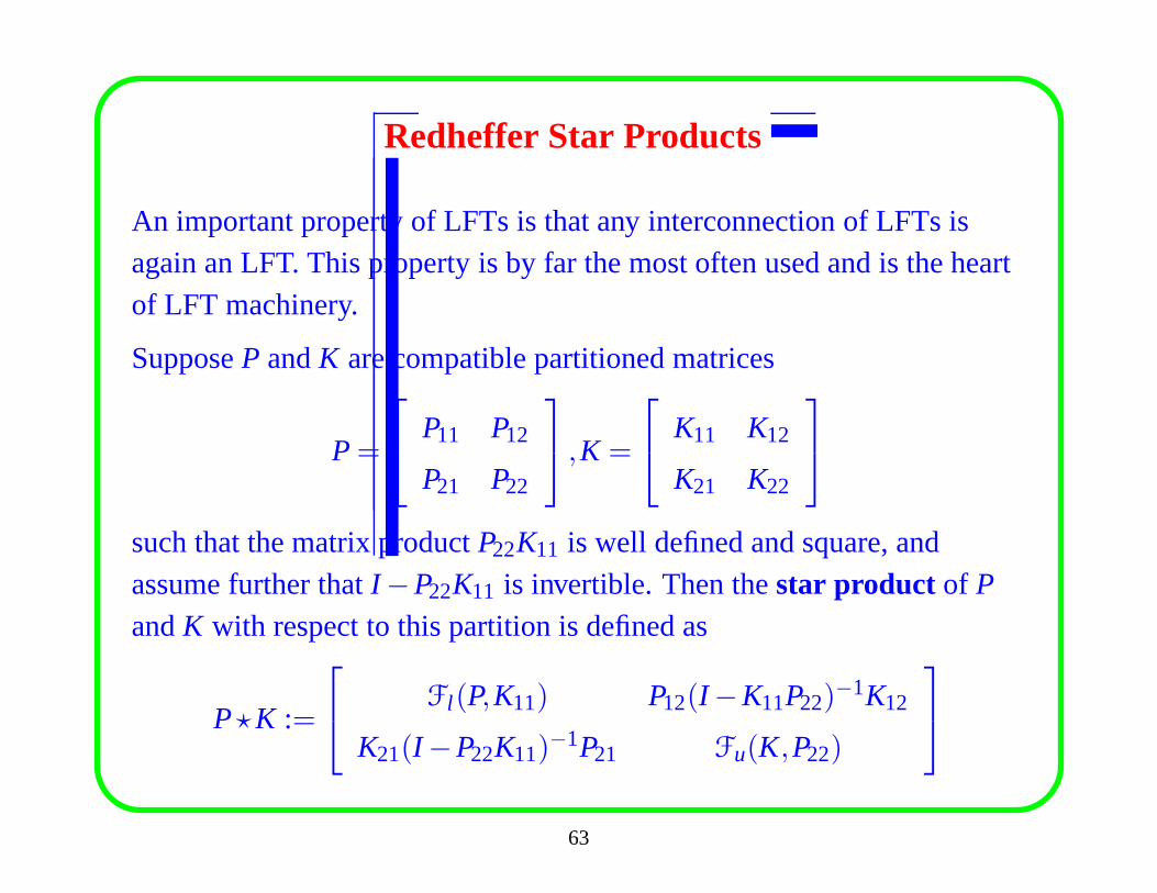
Redheffer Star Products

An important property of LFTs is that any interconnection ofLFTs isagain an LFT. This property is by far the most often used and isthe heartof LFT machinery.

SupposeP andK are compatible partitioned matrices

P=

P11 P12

P21 P22

,K =

K11 K12

K21 K22

such that the matrix productP22K11 is well defined and square, andassume further thatI −P22K11 is invertible. Then thestar product of P

andK with respect to this partition is defined as

P⋆K :=

Fl (P,K11) P12(I −K11P22)

−1K12

K21(I −P22K11)−1P21 Fu(K,P22)

63

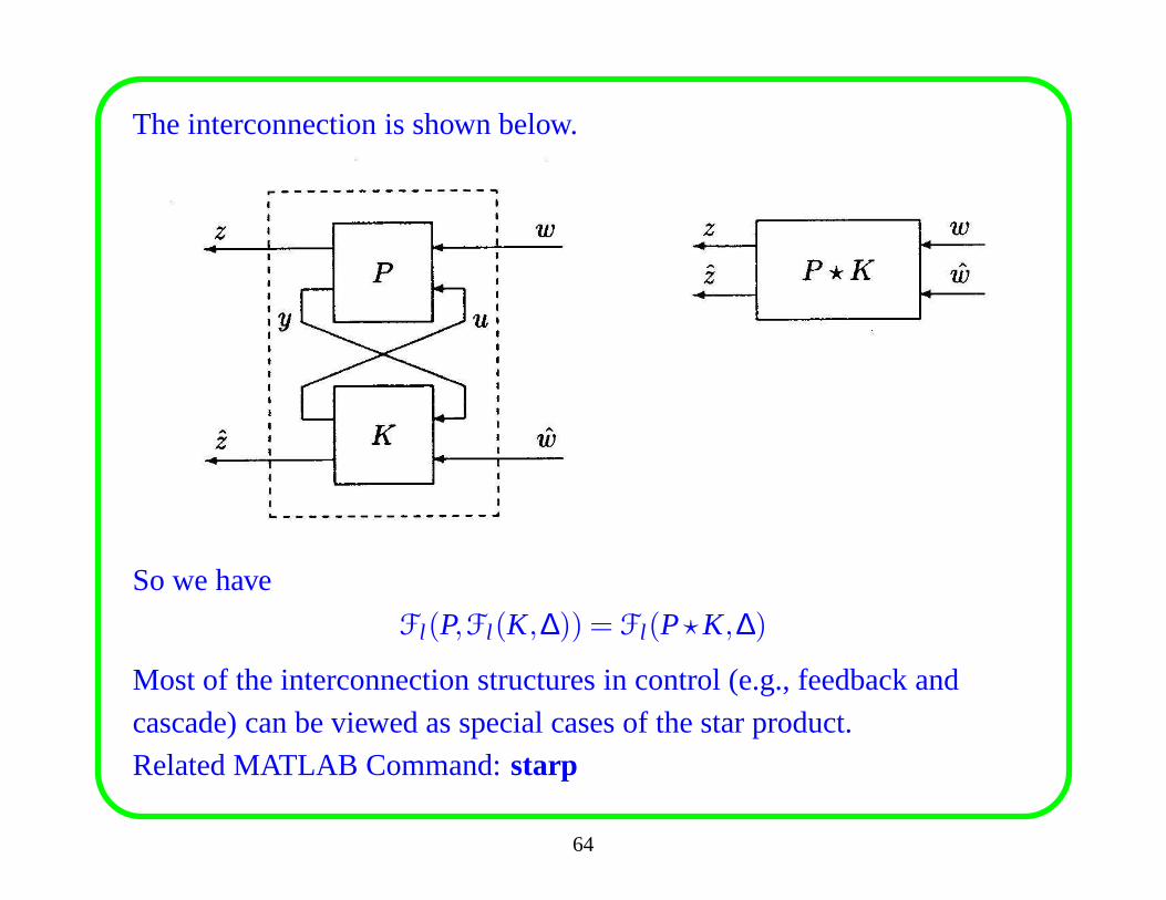
The interconnection is shown below.

So we have

Fl (P,Fl (K,∆)) = Fl (P⋆K,∆)

Most of the interconnection structures in control (e.g., feedback and

cascade) can be viewed as special cases of the star product.

Related MATLAB Command:starp

64

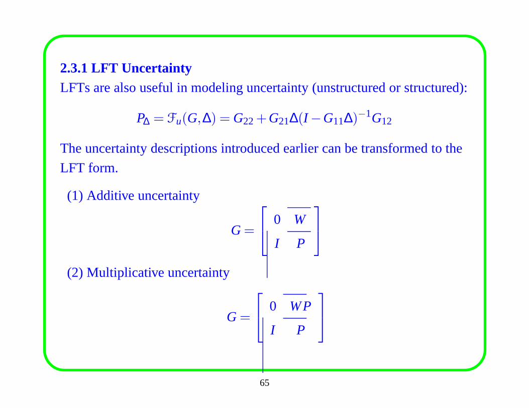
2.3.1 LFT UncertaintyLFTs are also useful in modeling uncertainty (unstructuredor structured):

P∆ = Fu(G,∆) = G22+G21∆(I −G11∆)−1G12

The uncertainty descriptions introduced earlier can be transformed to the

LFT form.

(1) Additive uncertainty

G=

0 W

I P

(2) Multiplicative uncertainty

G=

0 WP

I P

65

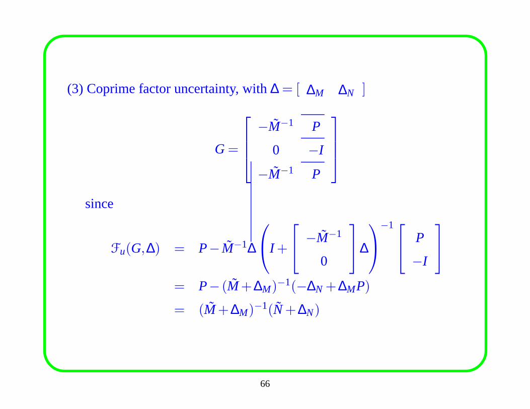
(3) Coprime factor uncertainty, with∆ = [ ∆M ∆N ]

G=

−M−1 P

0 −I

−M−1 P

since

Fu(G,∆) = P− M−1∆

I +

−M−1

0

∆

−1

P

−I

= P− (M+∆M)−1(−∆N +∆MP)

= (M+∆M)−1(N+∆N)

66

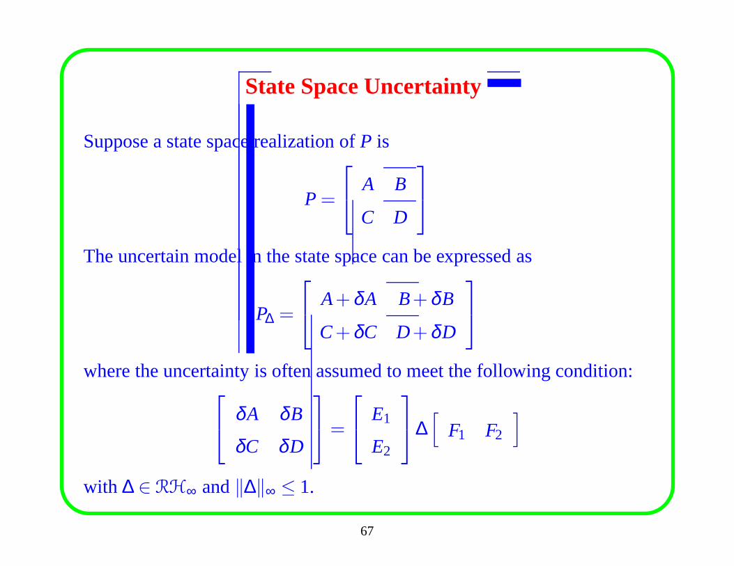
State Space Uncertainty

Suppose a state space realization ofP is

P=

A B

C D

The uncertain model in the state space can be expressed as

P∆ =

A+δA B+δB

C+δC D+δD

where the uncertainty is often assumed to meet the followingcondition:

δA δB

δC δD

=

E1

E2

∆[

F1 F2

]

with ∆ ∈ RH∞ and‖∆‖∞ ≤ 1.

67

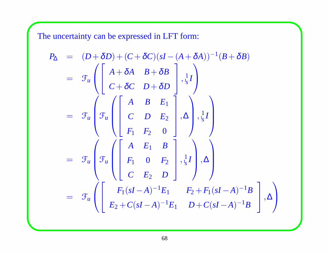
The uncertainty can be expressed in LFT form:

P∆ = (D+δD)+(C+δC)(sI− (A+δA))−1(B+δB)

= Fu

A+δA B+δB

C+δC D+δD

, 1sI

= Fu

Fu

A B E1

C D E2

F1 F2 0

,∆

, 1

sI

= Fu

Fu

A E1 B

F1 0 F2

C E2 D

, 1

sI

,∆

= Fu

F1(sI−A)−1E1 F2+F1(sI−A)−1B

E2+C(sI−A)−1E1 D+C(sI−A)−1B

,∆

68

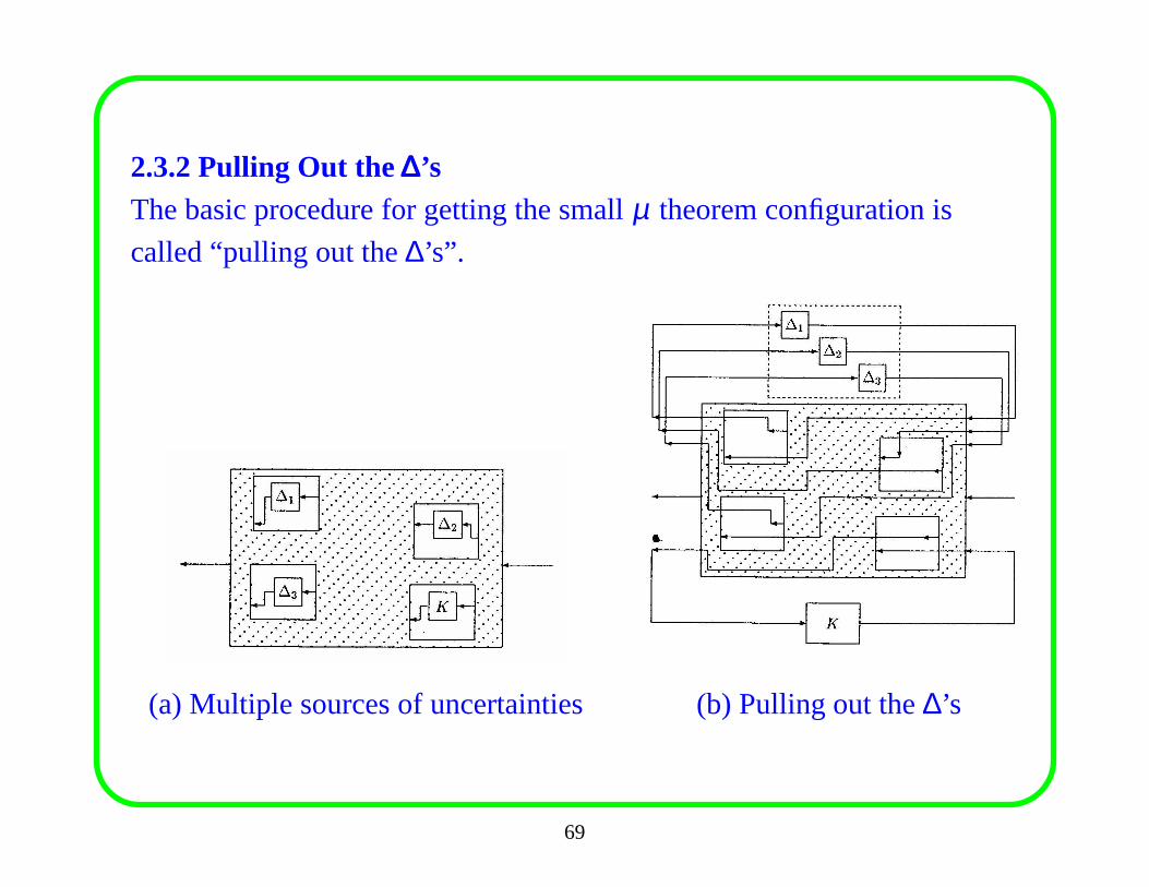
2.3.2 Pulling Out the∆∆∆’sThe basic procedure for getting the smallµ theorem configuration is

called “pulling out the∆’s”.

(a) Multiple sources of uncertainties (b) Pulling out the∆’s

69

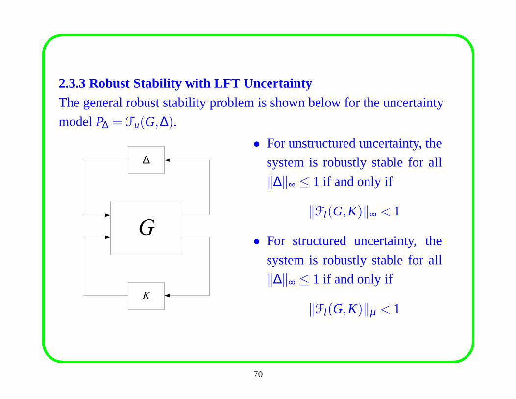
2.3.3 Robust Stability with LFT UncertaintyThe general robust stability problem is shown below for the uncertainty

modelP∆ = Fu(G,∆).

G

∆

K

• For unstructured uncertainty, the

system is robustly stable for all

‖∆‖∞ ≤ 1 if and only if

‖Fl (G,K)‖∞ < 1

• For structured uncertainty, the

system is robustly stable for all

‖∆‖∞ ≤ 1 if and only if

‖Fl (G,K)‖µ < 1

70

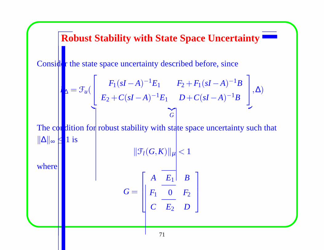
Robust Stability with State Space Uncertainty

Consider the state space uncertainty described before, since

P∆ = Fu(

F1(sI−A)−1E1 F2+F1(sI−A)−1B

E2+C(sI−A)−1E1 D+C(sI−A)−1B

︸ ︷︷ ︸

G

,∆)

The condition for robust stability with state space uncertainty such that‖∆‖∞ ≤ 1 is

‖Fl (G,K)‖µ < 1

where

G=

A E1 B

F1 0 F2

C E2 D

71

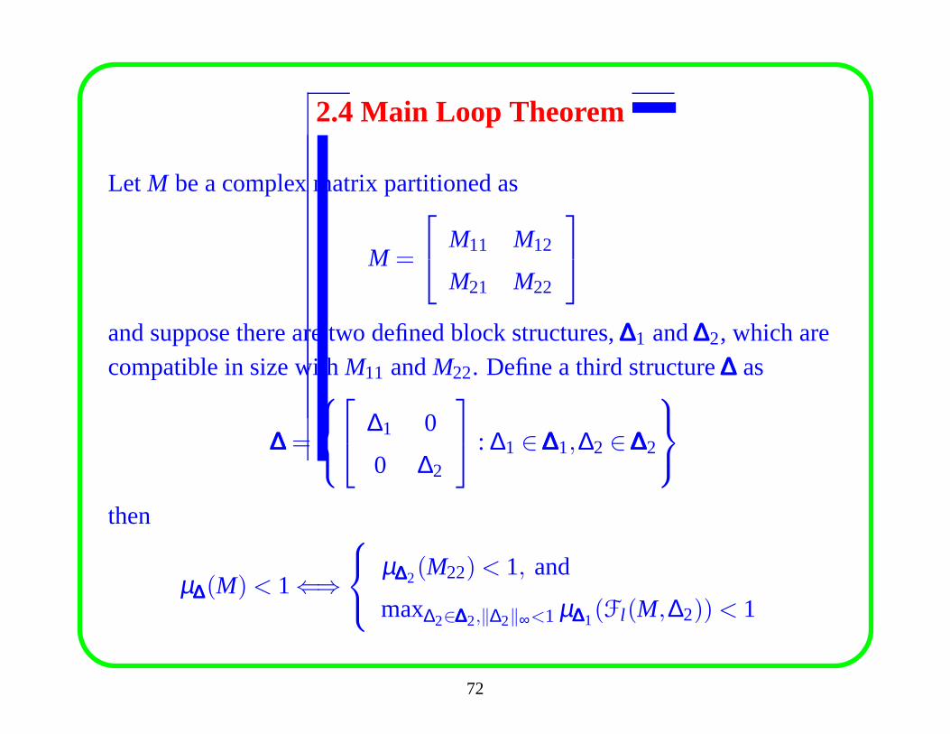
2.4 Main Loop Theorem

Let M be a complex matrix partitioned as

M =

M11 M12

M21 M22

and suppose there are two defined block structures,∆∆∆1 and∆∆∆2, which arecompatible in size withM11 andM22. Define a third structure∆∆∆ as

∆∆∆ =

∆1 0

0 ∆2

: ∆1 ∈∆∆∆1,∆2 ∈∆∆∆2

then

µ∆∆∆(M)< 1⇐⇒

µ∆∆∆2(M22)< 1, and

max∆2∈∆∆∆2,‖∆2‖∞<1 µ∆∆∆1(Fl (M,∆2))< 1

72

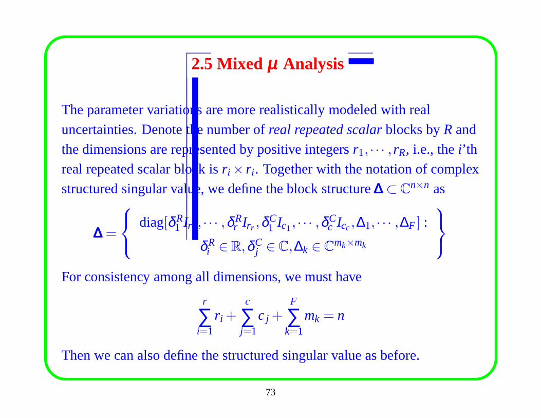
2.5 Mixed µµµ Analysis

The parameter variations are more realistically modeled with real

uncertainties. Denote the number ofreal repeated scalarblocks byRand

the dimensions are represented by positive integersr1, · · · , rR, i.e., thei’th

real repeated scalar block isr i × r i . Together with the notation of complexstructured singular value, we define the block structure∆∆∆ ⊂ Cn×n as

∆∆∆ =

diag[δ R1 Ir1, · · · ,δ R

r Irr ,δC1 Ic1, · · · ,δC

c Icc,∆1, · · · ,∆F ] :

δ Ri ∈ R,δC

j ∈ C,∆k ∈ Cmk×mk

For consistency among all dimensions, we must have

r

∑i=1

r i +c

∑j=1

c j +F

∑k=1

mk = n

Then we can also define the structured singular value as before.

73

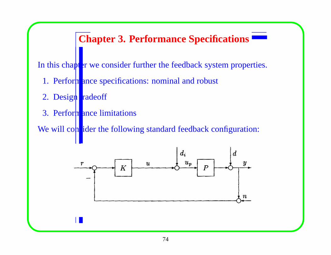
Chapter 3. Performance Specifications

In this chapter we consider further the feedback system properties.

1. Performance specifications: nominal and robust

2. Design tradeoff

3. Performance limitations

We will consider the following standard feedback configuration:

74

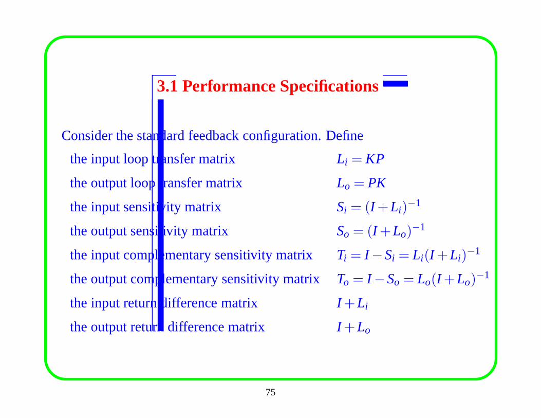
3.1 Performance Specifications

Consider the standard feedback configuration. Define

the input loop transfer matrix Li = KP

the output loop transfer matrix Lo = PK

the input sensitivity matrix Si = (I +Li)−1

the output sensitivity matrix So = (I +Lo)−1

the input complementary sensitivity matrix Ti = I −Si = Li(I +Li)−1

the output complementary sensitivity matrixTo = I −So = Lo(I +Lo)−1

the input return difference matrix I +Li

the output return difference matrix I +Lo

75

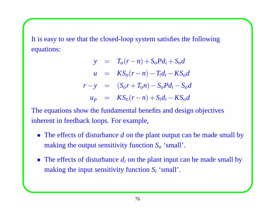
It is easy to see that the closed-loop system satisfies the following

equations:

y = To(r −n)+SoPdi +Sod

u = KSo(r −n)−Tidi −KSod

r −y = (Sor +Ton)−SoPdi −Sod

up = KSo(r −n)+Sidi −KSod

The equations show the fundamental benefits and design objectives

inherent in feedback loops. For example,

• The effects of disturbanced on the plant output can be made small by

making the output sensitivity functionSo ‘small’.

• The effects of disturbancedi on the plant input can be made small by

making the input sensitivity functionSi ‘small’.

76

With different assumption on the disturbance, we can formulate different

optimization problems for ‘optimal’ performance.

1. H∞H∞H∞ performance. The disturbance is assumed to be of bounded

power (RMS norm induced) or of bounded fuel (average-absolute

norm induced).

2. H2H2H2 performance. The disturbance is assumed to be white noise or

impulse, and the size ofy is taken as RMS value.

3. L1L1L1 performance. The disturbance is assumed to be bounded (L∞

induced).

77

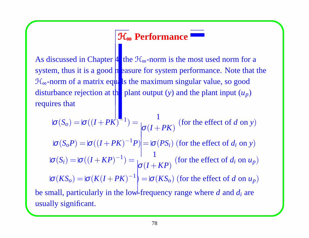
H∞H∞H∞ Performance

As discussed in Chapter 4, theH∞-norm is the most used norm for asystem, thus it is a good measure for system performance. Note that theH∞-norm of a matrix equals the maximum singular value, so gooddisturbance rejection at the plant output (y) and the plant input (up)requires that

σ(So) = σ((I +PK)−1) =1

σ(I +PK)(for the effect ofd on y)

σ(SoP) = σ((I +PK)−1P) = σ(PSi) (for the effect ofdi ony)

σ(Si) = σ((I +KP)−1) =1

σ(I +KP)(for the effect ofdi onup)

σ(KSo) = σ(K(I +PK)−1) = σ(KSo) (for the effect ofd onup)

be small, particularly in the low-frequency range whered anddi areusually significant.

78

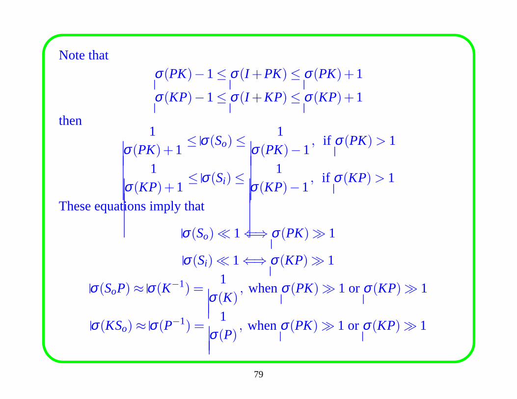
Note thatσ(PK)−1≤ σ(I +PK)≤ σ(PK)+1

σ(KP)−1≤ σ(I +KP)≤ σ(KP)+1

then1

σ(PK)+1≤ σ(So)≤

1σ(PK)−1

, if σ(PK)> 1

1σ(KP)+1

≤ σ(Si)≤1

σ(KP)−1, if σ(KP)> 1

These equations imply that

σ(So)≪ 1⇐⇒ σ(PK)≫ 1

σ(Si)≪ 1⇐⇒ σ(KP)≫ 1

σ(SoP)≈ σ(K−1) =1

σ(K), whenσ(PK)≫ 1 or σ(KP)≫ 1

σ(KSo)≈ σ(P−1) =1

σ(P), whenσ(PK)≫ 1 or σ(KP)≫ 1

79

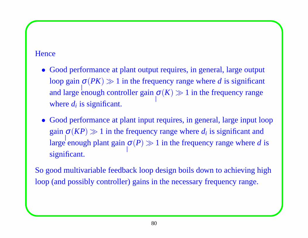
Hence

• Good performance at plant output requires, in general, large output

loop gainσ(PK)≫ 1 in the frequency range whered is significant

and large enough controller gainσ(K)≫ 1 in the frequency range

wheredi is significant.

• Good performance at plant input requires, in general, largeinput loop

gainσ(KP)≫ 1 in the frequency range wheredi is significant and

large enough plant gainσ(P)≫ 1 in the frequency range whered is

significant.

So good multivariable feedback loop design boils down to achieving high

loop (and possibly controller) gains in the necessary frequency range.

80

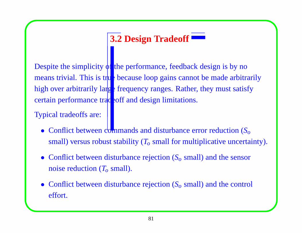
3.2 Design Tradeoff

Despite the simplicity of the performance, feedback designis by no

means trivial. This is true because loop gains cannot be madearbitrarily

high over arbitrarily large frequency ranges. Rather, theymust satisfy

certain performance tradeoff and design limitations.

Typical tradeoffs are:

• Conflict between commands and disturbance error reduction (So

small) versus robust stability (To small for multiplicative uncertainty).

• Conflict between disturbance rejection (So small) and the sensor

noise reduction (To small).

• Conflict between disturbance rejection (So small) and the control

effort.

81

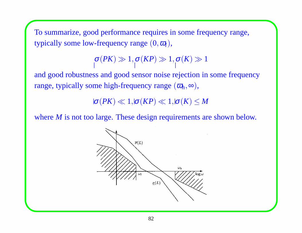
To summarize, good performance requires in some frequency range,typically some low-frequency range(0,ωl ),

σ(PK)≫ 1,σ(KP)≫ 1,σ(K)≫ 1

and good robustness and good sensor noise rejection in some frequencyrange, typically some high-frequency range(ωh,∞),

σ(PK)≪ 1,σ(KP)≪ 1,σ(K)≤ M

whereM is not too large. These design requirements are shown below.

82

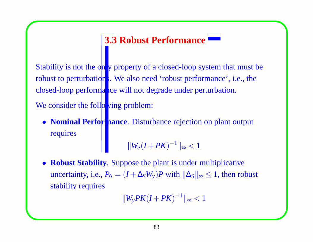
3.3 Robust Performance

Stability is not the only property of a closed-loop system that must be

robust to perturbations. We also need ‘robust performance’, i.e., the

closed-loop performance will not degrade under perturbation.

We consider the following problem:

• Nominal Performance. Disturbance rejection on plant output

requires

‖We(I +PK)−1‖∞ < 1

• Robust Stability. Suppose the plant is under multiplicative

uncertainty, i.e.,P∆ = (I +∆SWy)P with ‖∆S‖∞ ≤ 1, then robust

stability requires

‖WyPK(I +PK)−1‖∞ < 1

83

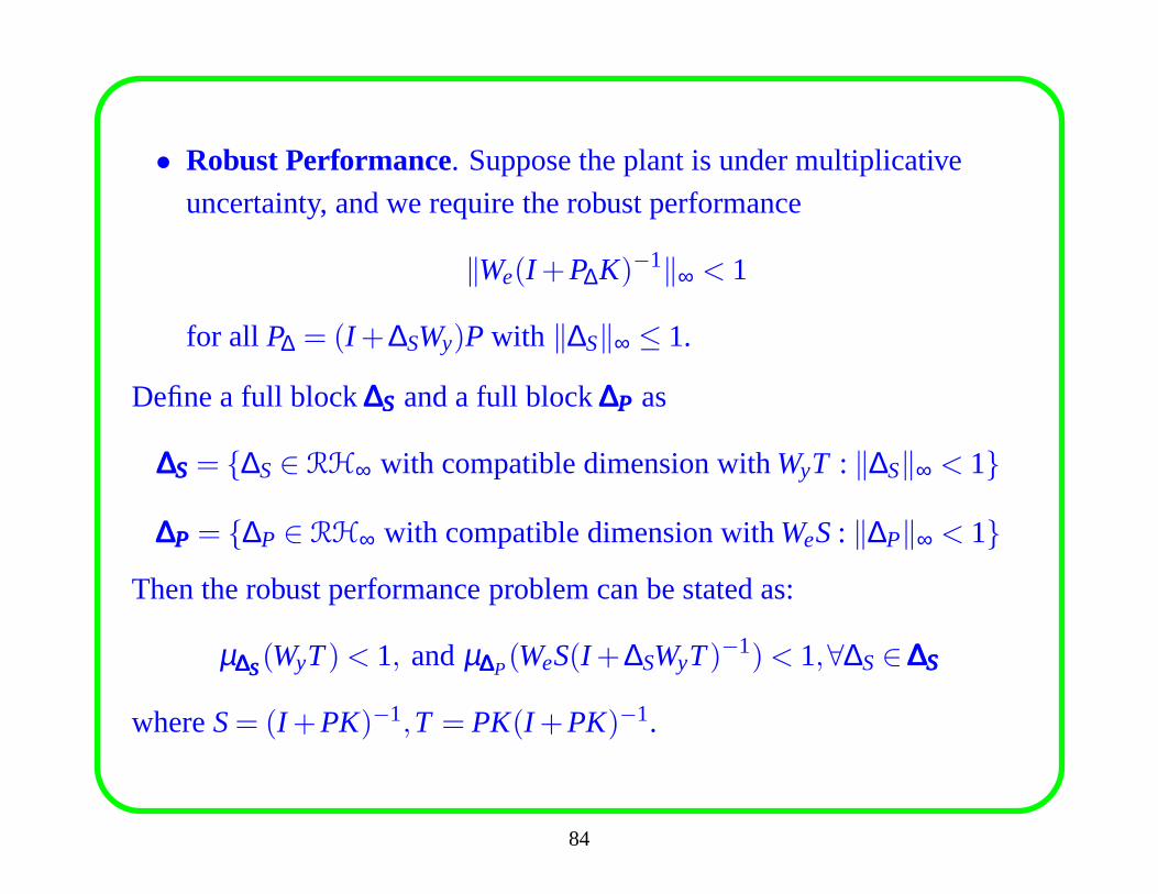
• Robust Performance. Suppose the plant is under multiplicative

uncertainty, and we require the robust performance

‖We(I +P∆K)−1‖∞ < 1

for all P∆ = (I +∆SWy)P with ‖∆S‖∞ ≤ 1.

Define a full block∆S∆S∆S and a full block∆P∆P∆P as

∆S∆S∆S= {∆S∈ RH∞ with compatible dimension withWyT : ‖∆S‖∞ < 1}

∆P∆P∆P = {∆P ∈ RH∞ with compatible dimension withWeS: ‖∆P‖∞ < 1}Then the robust performance problem can be stated as:

µ∆S∆S∆S(WyT)< 1, andµ∆∆∆P(WeS(I +∆SWyT)

−1)< 1,∀∆S∈∆S∆S∆S

whereS= (I +PK)−1,T = PK(I +PK)−1.

84

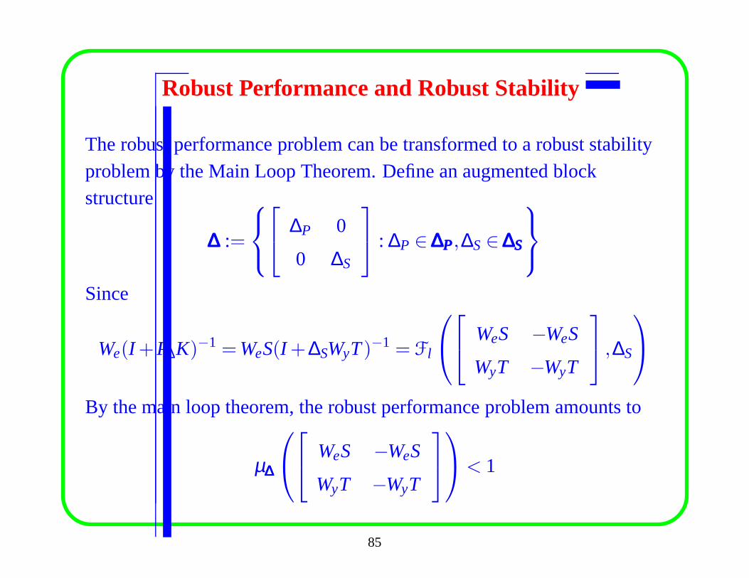
Robust Performance and Robust Stability

The robust performance problem can be transformed to a robust stabilityproblem by the Main Loop Theorem. Define an augmented blockstructure

∆∆∆ :=

∆P 0

0 ∆S

: ∆P ∈∆P∆P∆P,∆S∈∆S∆S∆S

Since

We(I +P∆K)−1 =WeS(I +∆SWyT)−1 = Fl

WeS −WeS

WyT −WyT

,∆S

By the main loop theorem, the robust performance problem amounts to

µ∆∆∆

WeS −WeS

WyT −WyT

< 1

85

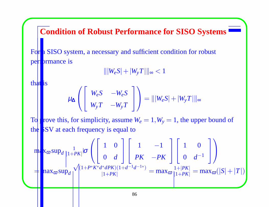
Condition of Robust Performance for SISO Systems

For a SISO system, a necessary and sufficient condition for robustperformance is

‖|WeS|+ |WyT|‖∞ < 1

that is

µ∆∆∆

WeS −WeS

WyT −WyT

= ‖|WeS|+ |WyT|‖∞

To prove this, for simplicity, assumeWe = 1,Wy = 1, the upper bound ofthe SSV at each frequency is equal to

maxω supd1

|1+PK|σ

1 0

0 d

1 −1

PK −PK

1 0

0 d−1

= maxω supd

√(1+P∗K∗d∗dPK)(1+d−1d−1∗)

|1+PK| = maxω1+|PK||1+PK| = maxω(|S|+ |T|)

86

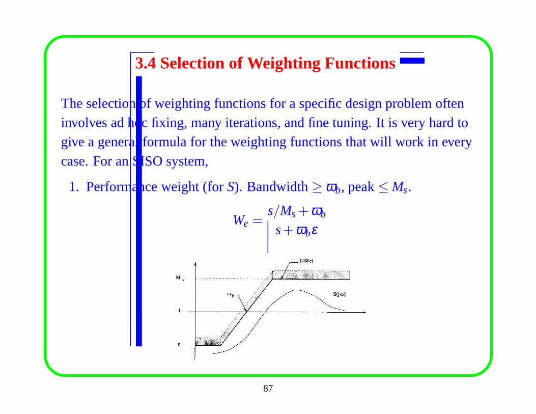
3.4 Selection of Weighting Functions

The selection of weighting functions for a specific design problem ofteninvolves ad hoc fixing, many iterations, and fine tuning. It isvery hard togive a general formula for the weighting functions that willwork in everycase. For an SISO system,

1. Performance weight (forS). Bandwidth≥ ωb, peak≤ Ms.

We =s/Ms+ωb

s+ωbε

87

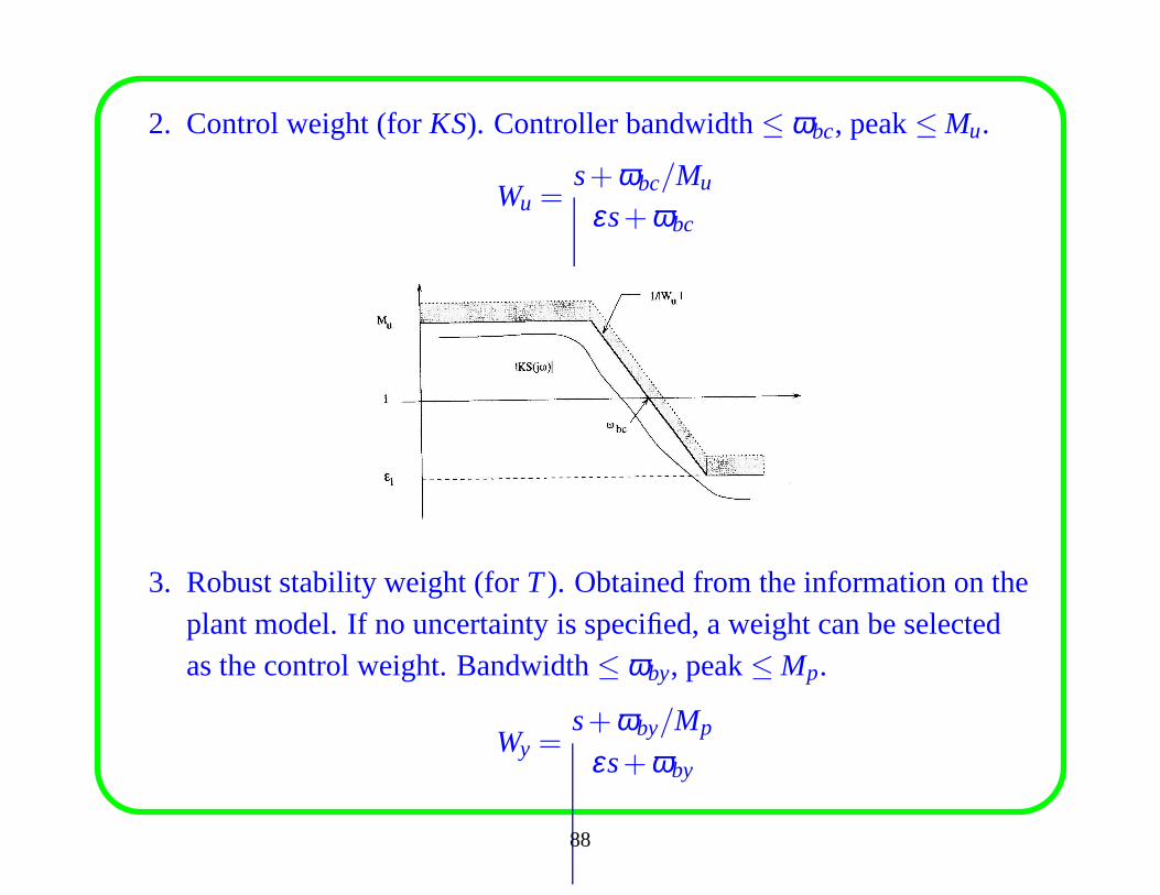
2. Control weight (forKS). Controller bandwidth≤ ωbc, peak≤ Mu.

Wu =s+ωbc/Mu

εs+ωbc

3. Robust stability weight (forT). Obtained from the information on theplant model. If no uncertainty is specified, a weight can be selectedas the control weight. Bandwidth≤ ωby, peak≤ Mp.

Wy =s+ωby/Mp

εs+ωby

88

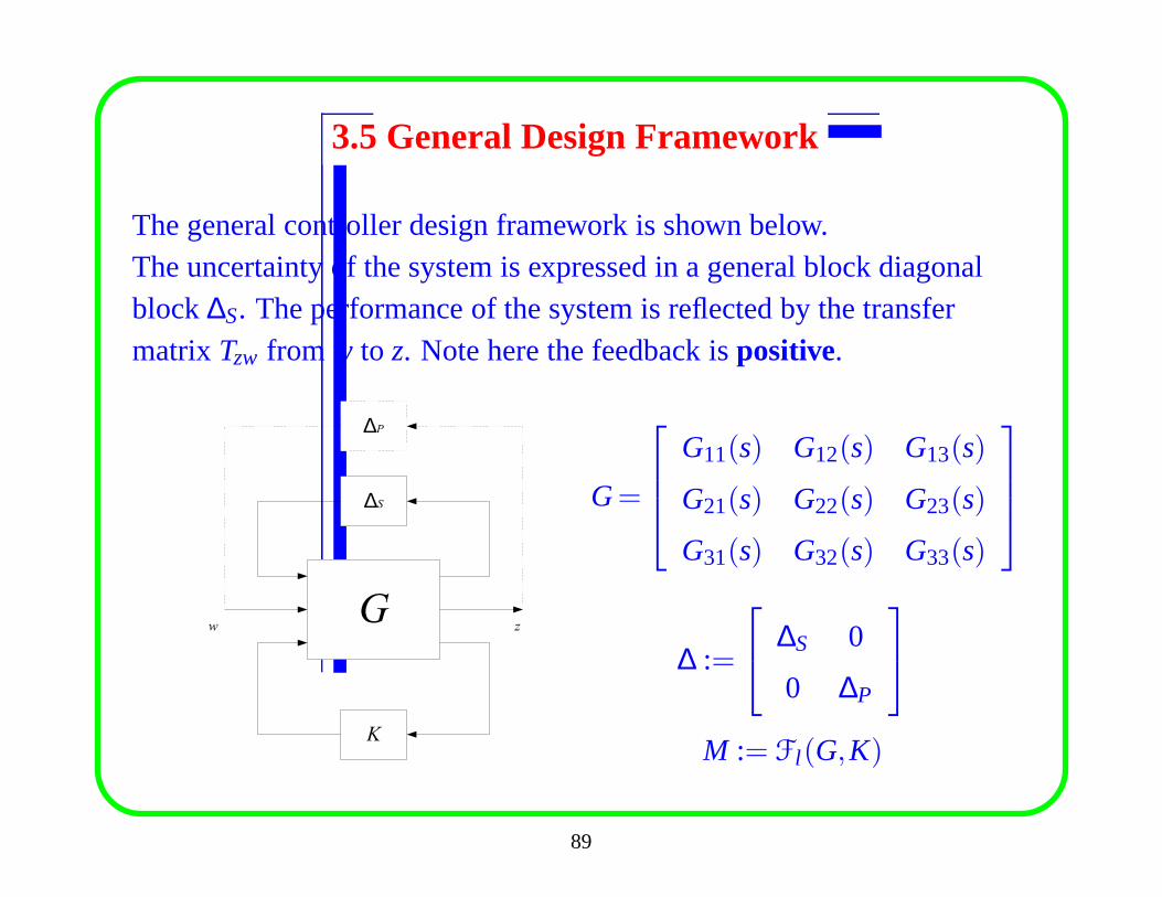
3.5 General Design Framework

The general controller design framework is shown below.The uncertainty of the system is expressed in a general blockdiagonalblock ∆S. The performance of the system is reflected by the transfermatrix Tzw from w to z. Note here the feedback ispositive.

G

∆S

K

w z

∆P

G=

G11(s) G12(s) G13(s)

G21(s) G22(s) G23(s)

G31(s) G32(s) G33(s)

∆ :=

∆S 0

0 ∆P

M := Fl (G,K)

89

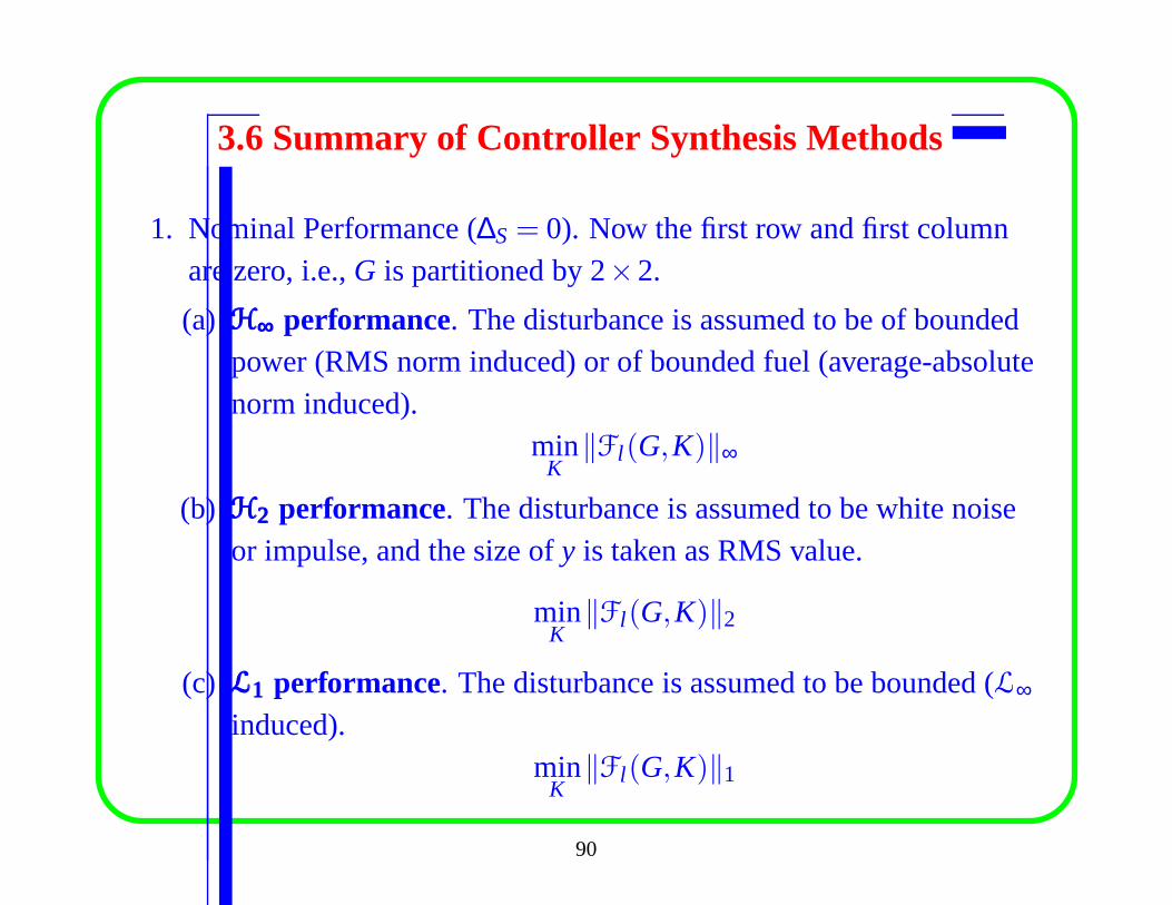
3.6 Summary of Controller Synthesis Methods

1. Nominal Performance (∆S= 0). Now the first row and first columnare zero, i.e.,G is partitioned by 2×2.

(a) H∞H∞H∞ performance. The disturbance is assumed to be of boundedpower (RMS norm induced) or of bounded fuel (average-absolutenorm induced).

minK

‖Fl (G,K)‖∞

(b) H2H2H2 performance. The disturbance is assumed to be white noiseor impulse, and the size ofy is taken as RMS value.

minK

‖Fl (G,K)‖2

(c) L1L1L1 performance. The disturbance is assumed to be bounded (L∞

induced).min

K‖Fl (G,K)‖1

90

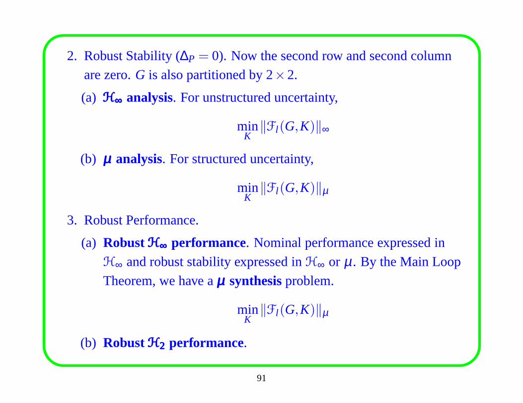
2. Robust Stability (∆P = 0). Now the second row and second columnare zero.G is also partitioned by 2×2.

(a) H∞H∞H∞ analysis. For unstructured uncertainty,

minK

‖Fl (G,K)‖∞

(b) µµµ analysis. For structured uncertainty,

minK

‖Fl (G,K)‖µ

3. Robust Performance.

(a) RobustH∞H∞H∞ performance. Nominal performance expressed in

H∞ and robust stability expressed inH∞ or µ. By the Main Loop

Theorem, we have aµµµ synthesisproblem.

minK

‖Fl (G,K)‖µ

(b) RobustH2H2H2 performance.

91

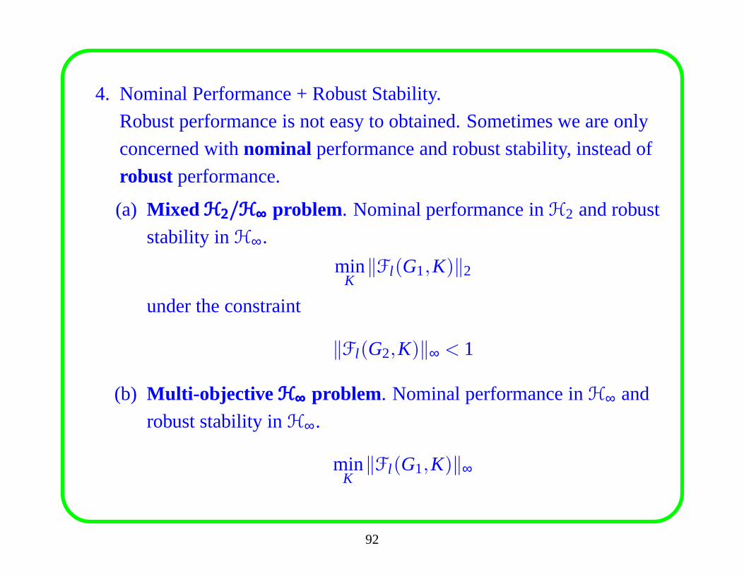
4. Nominal Performance + Robust Stability.

Robust performance is not easy to obtained. Sometimes we areonly

concerned withnominal performance and robust stability, instead of

robust performance.

(a) Mixed H2/H∞H2/H∞H2/H∞ problem. Nominal performance inH2 and robust

stability inH∞.

minK

‖Fl (G1,K)‖2

under the constraint

‖Fl (G2,K)‖∞ < 1

(b) Multi-objective H∞H∞H∞ problem. Nominal performance inH∞ and

robust stability inH∞.

minK

‖Fl (G1,K)‖∞

92

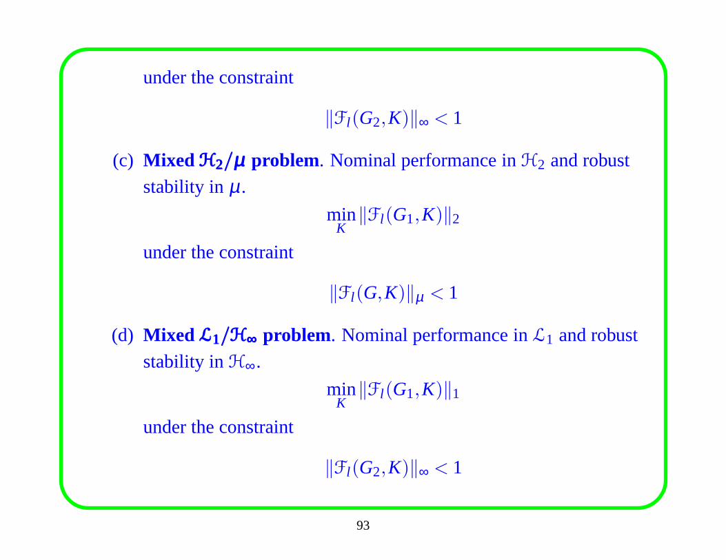
under the constraint

‖Fl (G2,K)‖∞ < 1

(c) Mixed H2/µH2/µH2/µ problem. Nominal performance inH2 and robust

stability in µ.

minK

‖Fl (G1,K)‖2

under the constraint

‖Fl (G,K)‖µ < 1

(d) Mixed L1/H∞L1/H∞L1/H∞ problem. Nominal performance inL1 and robust

stability inH∞.

minK

‖Fl (G1,K)‖1

under the constraint

‖Fl (G2,K)‖∞ < 1

93

Chapter 4. Robust Controller Synthesis

We have discussed performance specifications and tradeoffs. One simple

method to achieve performance specifications and tradeoffsis loop

shaping. The procedure of designing controllers by changing the shapes

of the (closed- and/or open-) loops of a system is calledloop shaping.There are two kinds of loop shaping methods:

(1) Shape the closed loopsS, T, or KS;

(2) Shape the open loopL.

We will discuss these methods in this chapter.

94

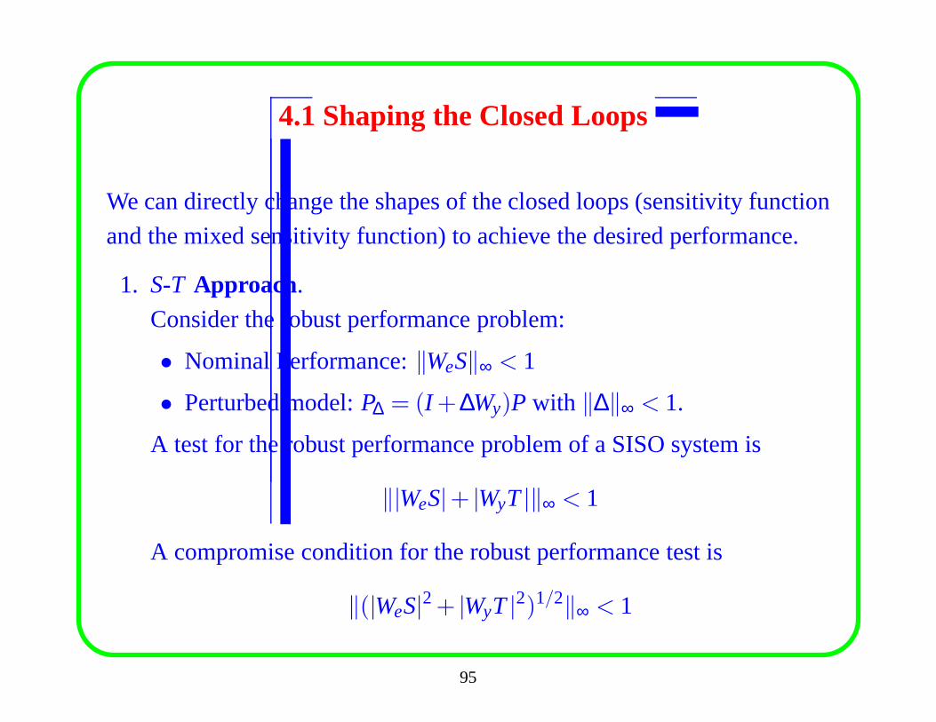
4.1 Shaping the Closed Loops

We can directly change the shapes of the closed loops (sensitivity function

and the mixed sensitivity function) to achieve the desired performance.

1. S-T Approach.

Consider the robust performance problem:

• Nominal Performance:‖WeS‖∞ < 1

• Perturbed model:P∆ = (I +∆Wy)P with ‖∆‖∞ < 1.

A test for the robust performance problem of a SISO system is

‖|WeS|+ |WyT|‖∞ < 1

A compromise condition for the robust performance test is

‖(|WeS|2+ |WyT|2)1/2‖∞ < 1

95

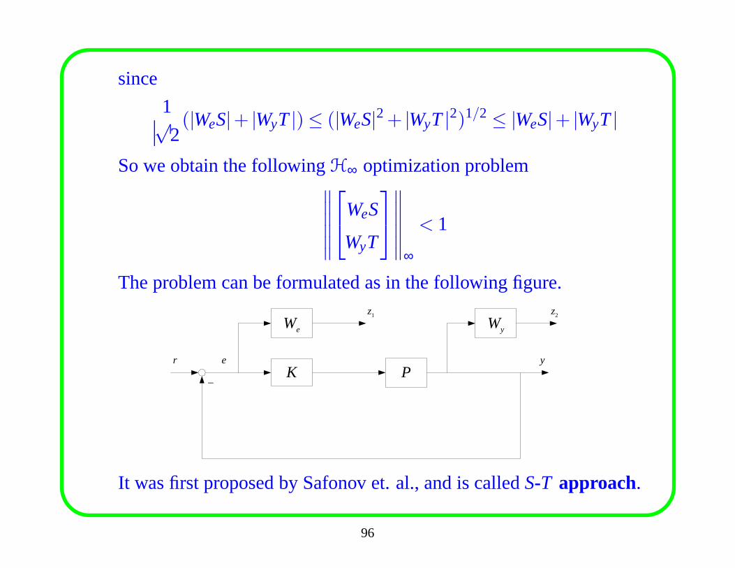
since

1√2(|WeS|+ |WyT|)≤ (|WeS|2+ |WyT|2)1/2 ≤ |WeS|+ |WyT|

So we obtain the followingH∞ optimization problem∥∥∥∥∥∥

WeS

WyT

∥∥∥∥∥∥

∞

< 1

The problem can be formulated as in the following figure.

K P

Wy

r

_

y

We

e

z1 z2

It was first proposed by Safonov et. al., and is calledS-T approach.

96

2. S-KSApproach.

Consider the robust performance problem:

• Nominal Performance:‖WeS‖∞ < 1

• Perturbed model:P∆ = P+∆Wu with ‖∆‖∞ < 1.

A test for the robust performance problem of a SISO system is

‖|WeS|+ |WuKS|‖∞ < 1

A compromise condition for the test is

‖(|WeS|2+ |WuKS|2)1/2‖∞ < 1

or ∥∥∥∥∥∥

WeS

WuKS

∥∥∥∥∥∥

∞

< 1

97

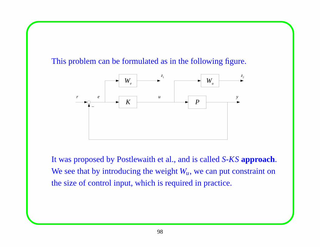
This problem can be formulated as in the following figure.

K P

Wu

r

_

y

We

e

z1 z2

u

It was proposed by Postlewaith et al., and is calledS-KSapproach.

We see that by introducing the weightWu, we can put constraint on

the size of control input, which is required in practice.

98

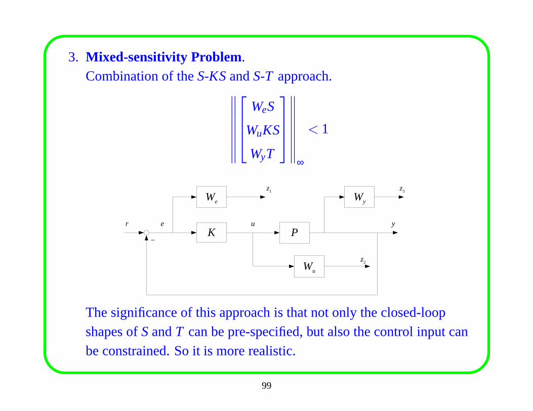
3. Mixed-sensitivity Problem.Combination of theS-KSandS-T approach.

∥∥∥∥∥∥∥∥

WeS

WuKS

WyT

∥∥∥∥∥∥∥∥

∞

< 1

K P

Wy

r

_

y

We

e

z1 z3

Wu

u

z2

The significance of this approach is that not only the closed-loopshapes ofSandT can be pre-specified, but also the control input canbe constrained. So it is more realistic.

99

Remarks on Mixed-Sensitivity Approach

• When the plant is strictly proper, i.e.,Dp = 0, then the ‘D12’ block of

theS-T problem is singular, thus violates the regularity assumption

of the standardH∞ problem. To solve this problem, we can perturb

Dp to Dp = Dp+ ε I with a smallε .

• TheS-KS is regular as long asDu is nonzero, which can always be

guaranteed. So it is with the mixed sensitivity problem.

• When the plant contains integrators, i.e.,Ap has zero eigenvalues,

then the regularity assumption (A1) or (A3) might not be guaranteed.

In this case we can perturbAp to Ap = Ap+ ε I with a smallε .

• TheH∞ controller of the mixed sensitivity problems always cancels

the stable poles of the plant with its transmission zeros, which is

undesired if the plant contains slow-mode poles.

100

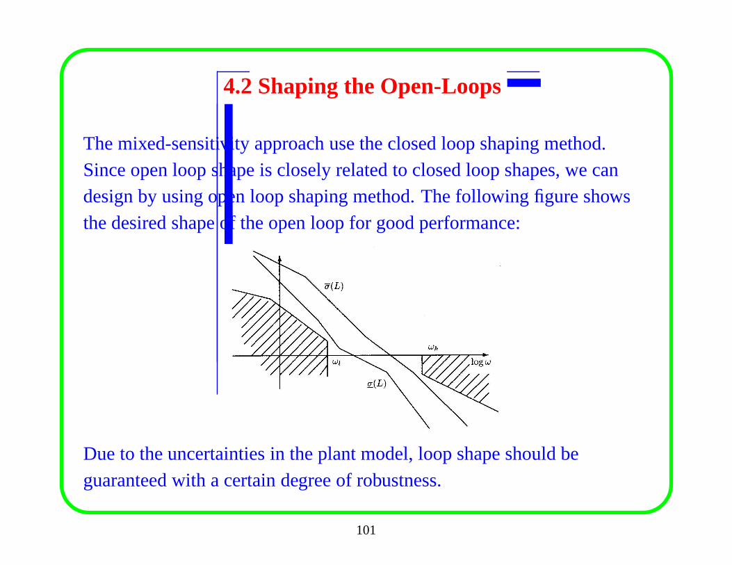
4.2 Shaping the Open-Loops

The mixed-sensitivity approach use the closed loop shapingmethod.Since open loop shape is closely related to closed loop shapes, we candesign by using open loop shaping method. The following figure showsthe desired shape of the open loop for good performance:

Due to the uncertainties in the plant model, loop shape should beguaranteed with a certain degree of robustness.

101

4.2.1 Loop ShapingH∞H∞H∞ DesignGiven a plantP, loop shapingH∞ design procedure goes as follows:

1. Loop Shaping. Pre-compensatorW1 and/or post-compensatorW2 are

used to shape the singular values ofP such that the shaped plant

P=W2PW1 has the desired open-loop shape.

2. Robust Stabilization. For the shaped plantP, find a controllerK

such that the robust stability marginε is maximized.

ε−1 = infK

∥∥∥∥∥∥

I

K

(I + PK)−1M−1

∥∥∥∥∥∥

∞

whereP= M−1N is an lcf ofP.

3. The final feedback controller is

K =W1KW2

102

It can be seen that in loop-shapingH∞ approach, the first step amounts todesign for performance, while the second step amounts to robustnessguaranty.

Some advantages of the loop shapingH∞ approach are as follows:

• The approach combines the classical loop shaping idea with therobust control idea.

• TheH∞ problem in step 2 is always regular and the infimum can becomputed explicitly without iteration. Further, the designedcontroller stabilizes all the plants in

P= {(M+∆M)−1(N+∆N) : ‖[ ∆M ∆N ]‖∞ < ε}

• There are no pole-zero cancellations between the plant and theH∞

controller.

• ε is a ‘design indicator’. A reasonable value indicates that the loopshapes can be well approximated together with good robust stability.

103

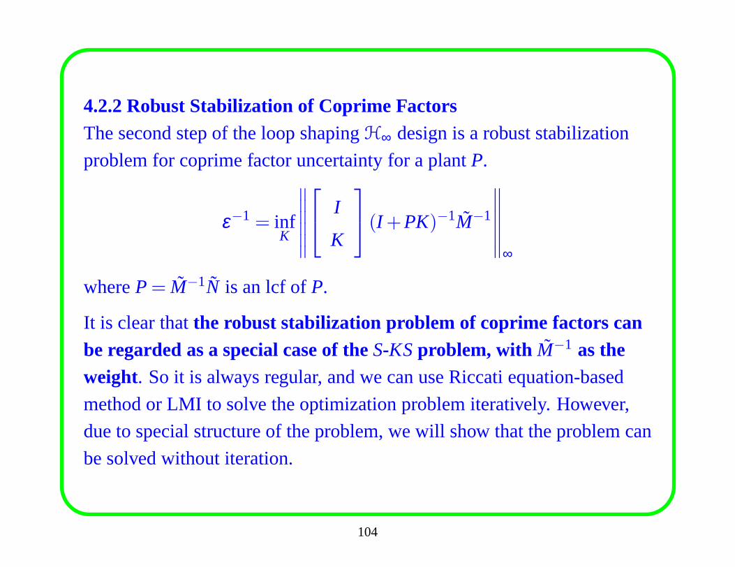
4.2.2 Robust Stabilization of Coprime FactorsThe second step of the loop shapingH∞ design is a robust stabilization

problem for coprime factor uncertainty for a plantP.

ε−1 = infK

∥∥∥∥∥∥

I

K

(I +PK)−1M−1

∥∥∥∥∥∥

∞

whereP= M−1N is an lcf ofP.

It is clear thatthe robust stabilization problem of coprime factors canbe regarded as a special case of theS-KSproblem, with M−1 as theweight. So it is always regular, and we can use Riccati equation-based

method or LMI to solve the optimization problem iteratively. However,

due to special structure of the problem, we will show that theproblem can

be solved without iteration.

104

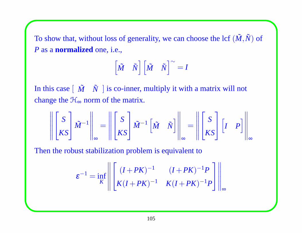
To show that, without loss of generality, we can choose the lcf (M, N) of

P as anormalized one, i.e.,[

M N][

M N]∼

= I

In this case[ M N ] is co-inner, multiply it with a matrix will not

change theH∞ norm of the matrix.∥∥∥∥∥∥

S

KS

M−1

∥∥∥∥∥∥

∞

=

∥∥∥∥∥∥

S

KS

M−1[

M N]

∥∥∥∥∥∥

∞

=

∥∥∥∥∥∥

S

KS

[

I P]

∥∥∥∥∥∥

∞

Then the robust stabilization problem is equivalent to

ε−1 = infK

∥∥∥∥∥∥

(I +PK)−1 (I +PK)−1P

K(I +PK)−1 K(I +PK)−1P

∥∥∥∥∥∥

∞

105

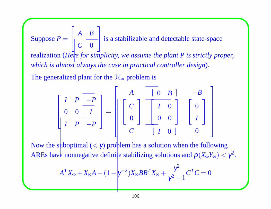
SupposeP=

A B

C 0

is a stabilizable and detectable state-space

realization (Here for simplicity, we assume the plant P is strictly proper,

which is almost always the case in practical controller design).

The generalized plant for theH∞ problem is

I P −P

0 0 I

I P −P

=

A [ 0 B ] −B

C

0

I 0

0 0

0

I

C [ I 0 ] 0

Now the suboptimal (< γ) problem has a solution when the followingAREs have nonnegative definite stabilizing solutions andρ(X∞Y∞)< γ2.

ATX∞ +X∞A− (1− γ−2)X∞BBTX∞ +γ2

γ2−1CTC= 0

106

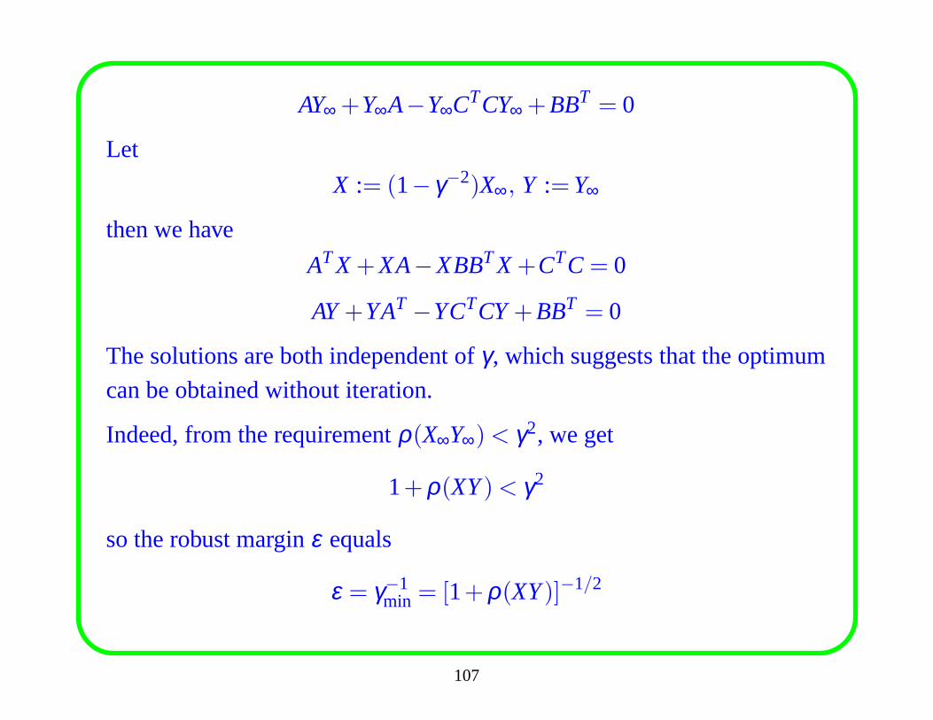
AY∞ +Y∞A−Y∞CTCY∞ +BBT = 0

Let

X := (1− γ−2)X∞, Y :=Y∞

then we have

ATX+XA−XBBTX+CTC= 0

AY+YAT −YCTCY+BBT = 0

The solutions are both independent ofγ, which suggests that the optimum

can be obtained without iteration.

Indeed, from the requirementρ(X∞Y∞)< γ2, we get

1+ρ(XY)< γ2

so the robust marginε equals

ε = γ−1min = [1+ρ(XY)]−1/2

107

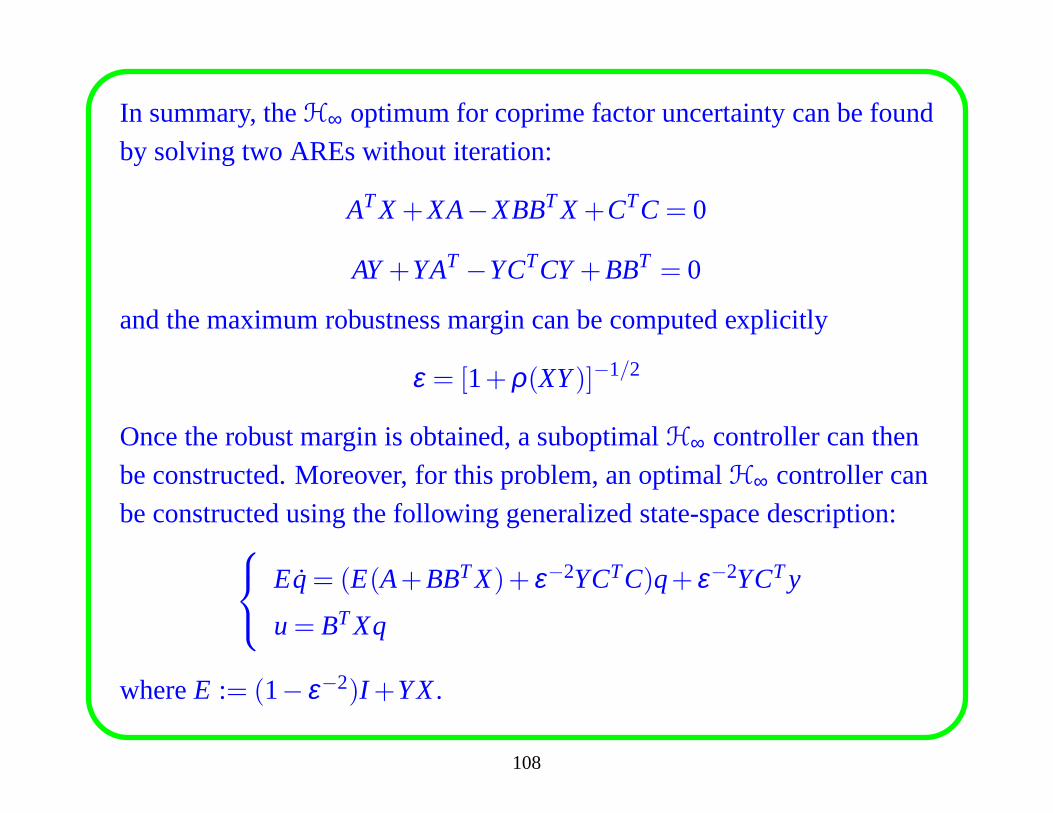
In summary, theH∞ optimum for coprime factor uncertainty can be found

by solving two AREs without iteration:

ATX+XA−XBBTX+CTC= 0

AY+YAT −YCTCY+BBT = 0

and the maximum robustness margin can be computed explicitly

ε = [1+ρ(XY)]−1/2

Once the robust margin is obtained, a suboptimalH∞ controller can then

be constructed. Moreover, for this problem, an optimalH∞ controller can

be constructed using the following generalized state-space description:

Eq= (E(A+BBTX)+ ε−2YCTC)q+ ε−2YCTy

u= BTXq

whereE := (1− ε−2)I +YX.

108

4.2.3 Design Procedure ofH∞H∞H∞ Loop-Shaping

1. Scale the plant outputs and inputs. This is very importantfor mostdesign procedures and is sometimes forgotten. In general, scalingimproves the conditioning of the design problem, it enablesmeaningful analysis to be made of the robustness propertiesof thefeedback system in the frequency domain.

2. Order the inputs and outputs so that the plant is as diagonal aspossible. The relative gain array (RGA) can be useful here.

3. Select the pre- and/or postcompensators to obtain the shaped plantP=W2PW1. The desired shapes normally mean high gain at lowfrequencies, roll-off rates of approximately 20 dB/decadeat thedesired bandwidth(s), and higher rates at high frequencies.

(a) W2 is usually chosen as a constant, reflecting the relativeimportance of the outputs to be controlled.

109

(b) In generalW1 has the formW1 =WpWaWg.

• Wp contains dynamic shaping. Integral action for lowfrequency performance; phase-advance for reducing the roll-offrates at crossover; and phase-lag to increase the roll-off rates athigh frequencies should all be placed inWp if desired.

• Wa is a constant that aligns the singular values at a desiredbandwidth (optional). This is effectively a constant decouplerand should not be used if the plant is ill-conditioned in terms oflarge RGA elements.

• Wg is an additional gain matrix to provide control over actuatorusage (optional). It is diagonal and adjusted so that the actuatorrate limits are not exceeded for reference demands and typicaldisturbances on the scaled plant outputs.

4. Robustly stabilize the shaped plantP. If the robust margin is toosmall (ε < 0.25), then go back to the previous step and modify theweights.

110

5. Analyze the design and if all the specifications are not metmake

further modifications to the weights.

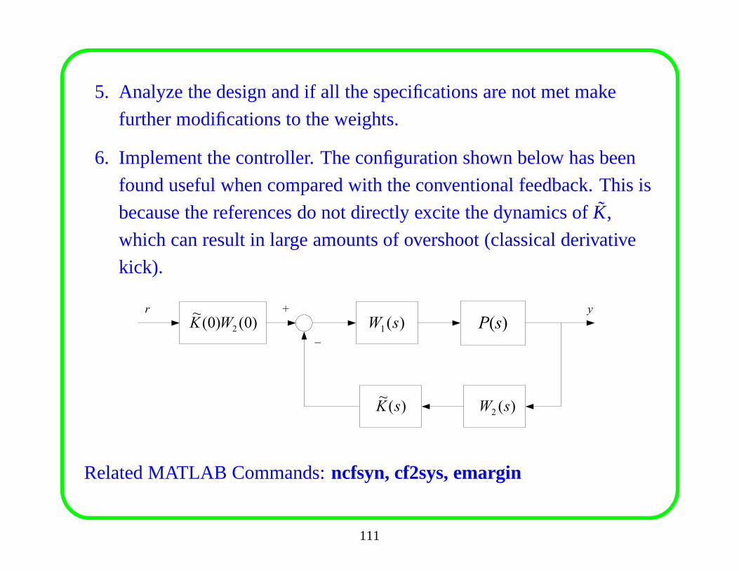
6. Implement the controller. The configuration shown below has been

found useful when compared with the conventional feedback.This is

because the references do not directly excite the dynamics of K,

which can result in large amounts of overshoot (classical derivative

kick).

P(s)r y

_

+

)(~sK

)(1 sW

)(2 sW

)0()0(~

2WK

Related MATLAB Commands:ncfsyn, cf2sys, emargin

111

4.2.4 Guidelines for Loop Shaping DesignSome guidelines for the loop-shaping design:

• The loop transfer function should be shaped in such a way thatit has

low gain around the frequency of the modulus of any right-half plane

zeroz. Typically, it requires that the crossover frequency be much

smaller than the modulus of the right-half plane zero; say,ωc <|z|2

for any real zero andωc < |z| for any complex zero with a much

larger imaginary part than the real part.

• The loop transfer function should have a large gain around the

frequency of the modulus of any right-half plane pole.

• The loop transfer function should not have a large slope nearthe

crossover frequencies.

These guidelines are consistent with the rules used in classical control

theory.

112

Chapter 5. Model Reduction

Simple linear models/controllers are preferred over complex ones incontrol system design for some obvious reasons:

(1) Simple models are much easier to do analysis and synthesis with.

(2) Simple controllers are easier to implement and are more reliable.

(3) In the case of infinite dimensional system, the mode/controllerapproximation becomes essential.

A model order-reduction problem can, in general, be stated as follows:Given a full-order model G(s), find a low-order model (say, an rth ordermodel Gr ), such that G and Gr are close in some sense. There are manyways to define the closeness of an approximation. The most used norm istheL∞-norm. So the model reduction problem can be formulated as

infdeg(Gr )<r

‖G−Gr‖∞

113

5.1 Truncation Methods

Truncation methods of model reduction seek to remove or truncateunimportant states from state-space models. There are two options:

1. State-space truncation.Consider a linear, time-invariant system with the realization

G=

x(t) = Ax(t)+Bu(t), x(0) = x0

y(t) = Cx(t)+Du(t)

Divide the state vectorx into two components:

x(t) =

x1(t)

x2(t)

where ther-vectorx1(t) contains the components to be retained, andthe(n− r)-vectorx2(t) contains the components to be discarded.

114

Now partition the matricesA, B andC conformably withx to obtain

A=

A11 A12

A21 A22

,B=

B1

B2

,C=[

C1 C2

]

By omitting the states and dynamics associated withx2(t), we obtain

the low-order system

Gr =

p(t) = A11p(t)+B1u(t), p(0) = p0

q(t) = C1p(t)+Du(t)

Therth-order truncation of the realization(A,B,C,D) is given by

Tr(A,B,C,D) = (A11,B1,C1,D)

115

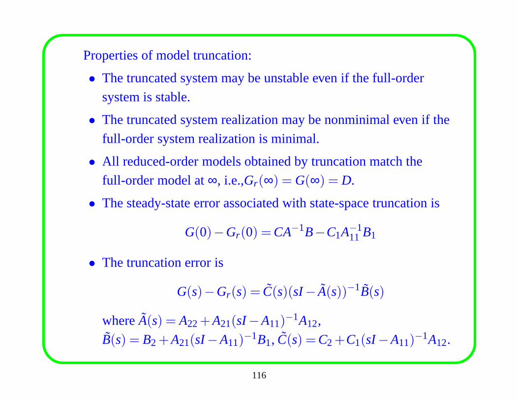
Properties of model truncation:

• The truncated system may be unstable even if the full-order

system is stable.

• The truncated system realization may be nonminimal even if the

full-order system realization is minimal.

• All reduced-order models obtained by truncation match the

full-order model at∞, i.e.,Gr(∞) = G(∞) = D.

• The steady-state error associated with state-space truncation is

G(0)−Gr(0) =CA−1B−C1A−111 B1

• The truncation error is

G(s)−Gr(s) = C(s)(sI− A(s))−1B(s)

whereA(s) = A22+A21(sI−A11)−1A12,

B(s) = B2+A21(sI−A11)−1B1, C(s) =C2+C1(sI−A11)

−1A12.

116

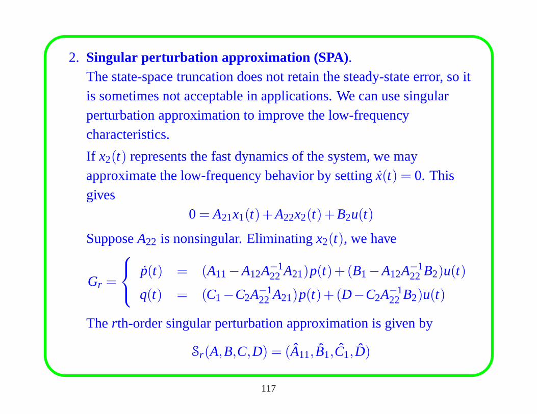
2. Singular perturbation approximation (SPA) .The state-space truncation does not retain the steady-state error, so itis sometimes not acceptable in applications. We can use singularperturbation approximation to improve the low-frequencycharacteristics.

If x2(t) represents the fast dynamics of the system, we mayapproximate the low-frequency behavior by setting ˙x(t) = 0. Thisgives

0= A21x1(t)+A22x2(t)+B2u(t)

SupposeA22 is nonsingular. Eliminatingx2(t), we have

Gr =

p(t) = (A11−A12A−122 A21)p(t)+(B1−A12A

−122 B2)u(t)

q(t) = (C1−C2A−122 A21)p(t)+(D−C2A−1

22 B2)u(t)

Therth-order singular perturbation approximation is given by

Sr(A,B,C,D) = (A11, B1,C1, D)

117

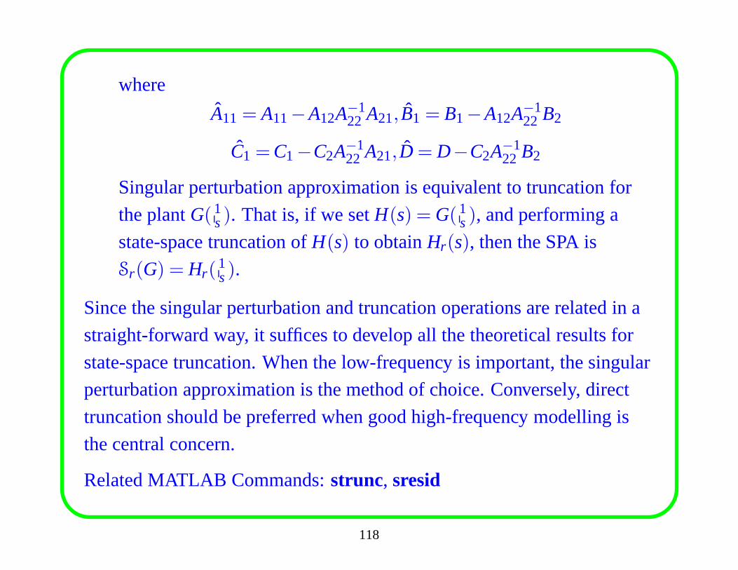
where

A11 = A11−A12A−122 A21, B1 = B1−A12A

−122 B2

C1 =C1−C2A−122 A21, D = D−C2A−1

22 B2

Singular perturbation approximation is equivalent to truncation for

the plantG(1s). That is, if we setH(s) = G(1

s), and performing a

state-space truncation ofH(s) to obtainHr(s), then the SPA is

Sr(G) = Hr(1s).

Since the singular perturbation and truncation operationsare related in a

straight-forward way, it suffices to develop all the theoretical results for

state-space truncation. When the low-frequency is important, the singular

perturbation approximation is the method of choice. Conversely, direct

truncation should be preferred when good high-frequency modelling is

the central concern.

Related MATLAB Commands:strunc, sresid

118

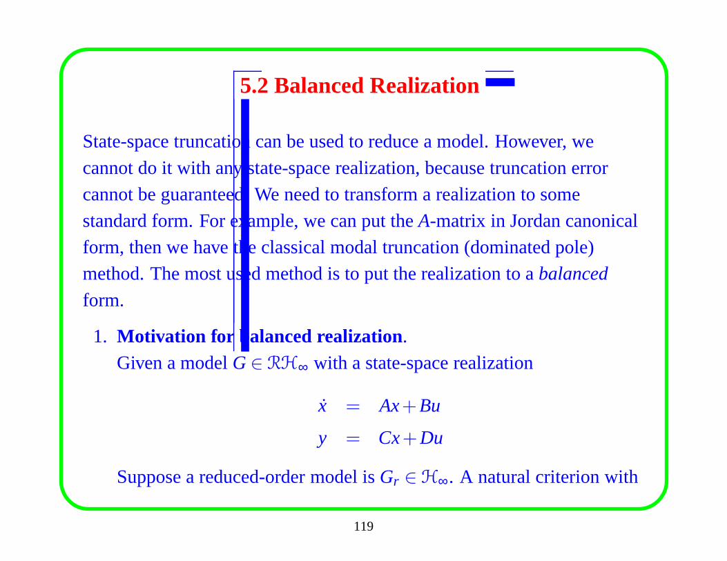
5.2 Balanced Realization

State-space truncation can be used to reduce a model. However, we

cannot do it with any state-space realization, because truncation errorcannot be guaranteed. We need to transform a realization to somestandard form. For example, we can put theA-matrix in Jordan canonicalform, then we have the classical modal truncation (dominated pole)method. The most used method is to put the realization to abalanced

form.

1. Motivation for balanced realization.

Given a modelG∈ RH∞ with a state-space realization

x = Ax+Bu

y = Cx+Du

Suppose a reduced-order model isGr ∈H∞. A natural criterion with

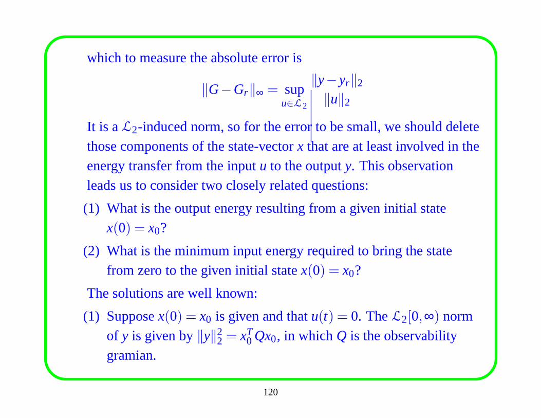
119

which to measure the absolute error is

‖G−Gr‖∞ = supu∈L2

‖y−yr‖2

‖u‖2

It is aL2-induced norm, so for the error to be small, we should deletethose components of the state-vectorx that are at least involved in theenergy transfer from the inputu to the outputy. This observationleads us to consider two closely related questions:

(1) What is the output energy resulting from a given initial statex(0) = x0?

(2) What is the minimum input energy required to bring the statefrom zero to the given initial statex(0) = x0?

The solutions are well known:

(1) Supposex(0) = x0 is given and thatu(t) = 0. TheL2[0,∞) normof y is given by‖y‖2

2 = xT0 Qx0, in whichQ is the observability

gramian.

120

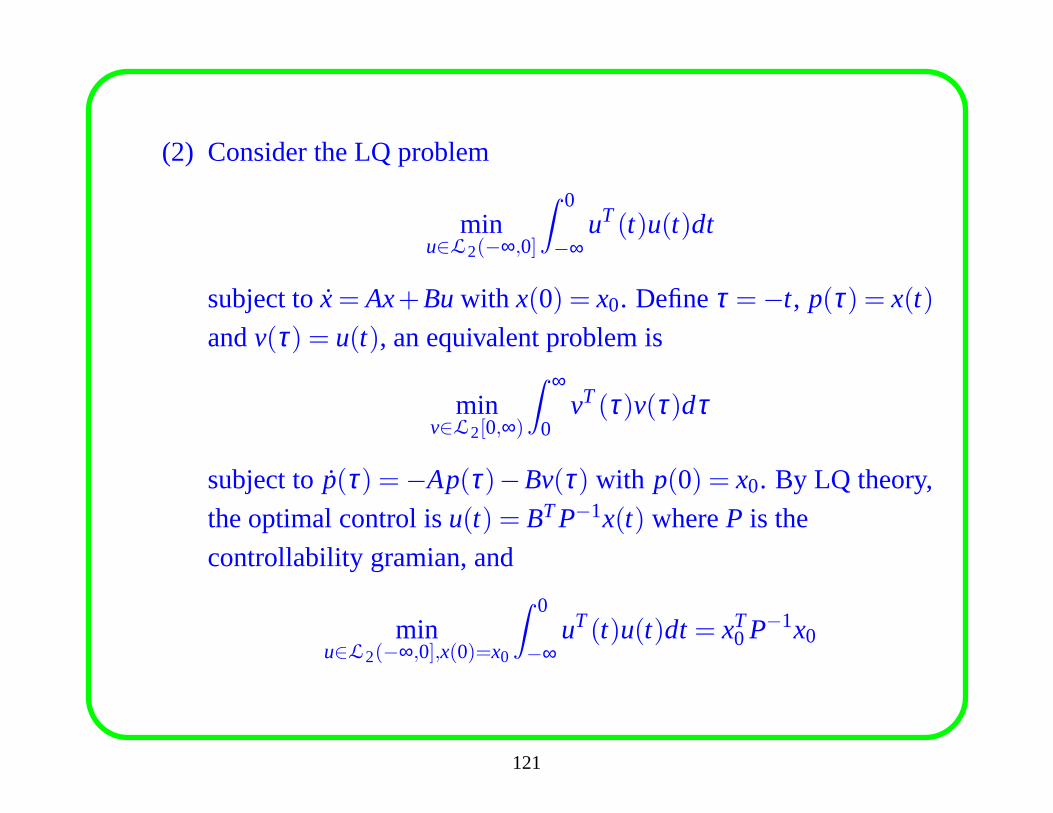
(2) Consider the LQ problem

minu∈L2(−∞,0]

∫ 0

−∞uT(t)u(t)dt

subject to ˙x= Ax+Buwith x(0) = x0. Defineτ =−t, p(τ) = x(t)

andv(τ) = u(t), an equivalent problem is

minv∈L2[0,∞)

∫ ∞

0vT(τ)v(τ)dτ

subject to ˙p(τ) =−Ap(τ)−Bv(τ) with p(0) = x0. By LQ theory,

the optimal control isu(t) = BTP−1x(t) whereP is the

controllability gramian, and

minu∈L2(−∞,0],x(0)=x0

∫ 0

−∞uT(t)u(t)dt = xT

0 P−1x0

121

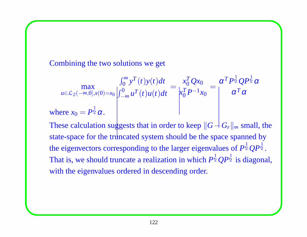
Combining the two solutions we get

maxu∈L2(−∞,0],x(0)=x0

∫ ∞0 yT(t)y(t)dt∫ 0−∞ uT(t)u(t)dt

=xT

0 Qx0

xT0 P−1x0

=αTP

12 QP

12 α

αTα

wherex0 = P12 α.

These calculation suggests that in order to keep‖G−Gr‖∞ small, the

state-space for the truncated system should be the space spanned by

the eigenvectors corresponding to the larger eigenvalues of P12 QP

12 .

That is, we should truncate a realization in whichP12 QP

12 is diagonal,

with the eigenvalues ordered in descending order.

122

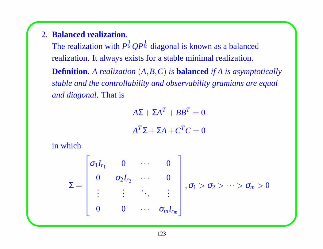
2. Balanced realization.The realization withP

12 QP

12 diagonal is known as a balanced

realization. It always exists for a stable minimal realization.

Definition. A realization(A,B,C) is balancedif A is asymptotically

stable and the controllability and observability gramiansare equal

and diagonal. That is

AΣ+ΣAT +BBT = 0

ATΣ+ΣA+CTC= 0

in which

Σ =

σ1Ir1 0 · · · 0

0 σ2Ir2 · · · 0...

......

...

0 0 · · · σmIrm

,σ1 > σ2 > · · ·> σm > 0

123

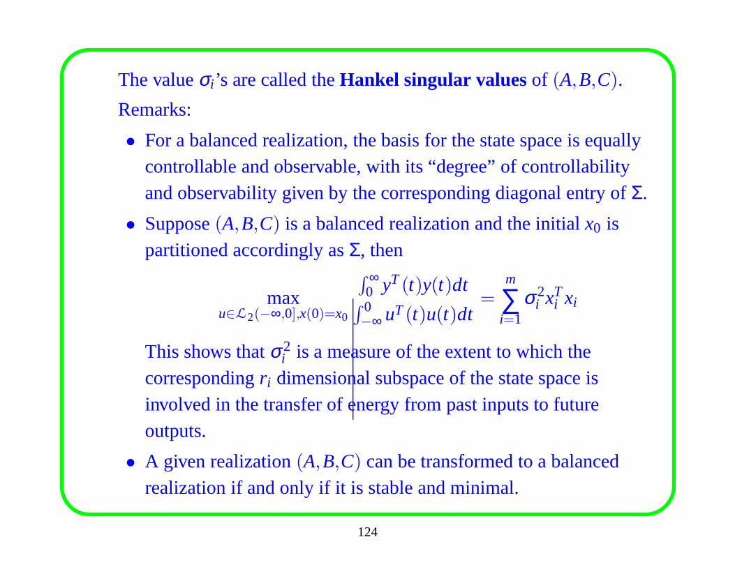
The valueσi ’s are called theHankel singular valuesof (A,B,C).

Remarks:

• For a balanced realization, the basis for the state space is equallycontrollable and observable, with its “degree” of controllabilityand observability given by the corresponding diagonal entry of Σ.

• Suppose(A,B,C) is a balanced realization and the initialx0 ispartitioned accordingly asΣ, then

maxu∈L2(−∞,0],x(0)=x0

∫ ∞0 yT(t)y(t)dt∫ 0−∞ uT(t)u(t)dt

=m

∑i=1

σ2i xT

i xi

This shows thatσ2i is a measure of the extent to which the

correspondingr i dimensional subspace of the state space isinvolved in the transfer of energy from past inputs to futureoutputs.

• A given realization(A,B,C) can be transformed to a balancedrealization if and only if it is stable and minimal.

124

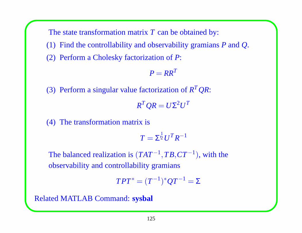
The state transformation matrixT can be obtained by:

(1) Find the controllability and observability gramiansP andQ.

(2) Perform a Cholesky factorization ofP:

P= RRT

(3) Perform a singular value factorization ofRTQR:

RTQR=UΣ2UT

(4) The transformation matrix is

T = Σ12UTR−1

The balanced realization is(TAT−1,TB,CT−1), with theobservability and controllability gramians

TPT∗ = (T−1)∗QT−1 = Σ

Related MATLAB Command:sysbal

125

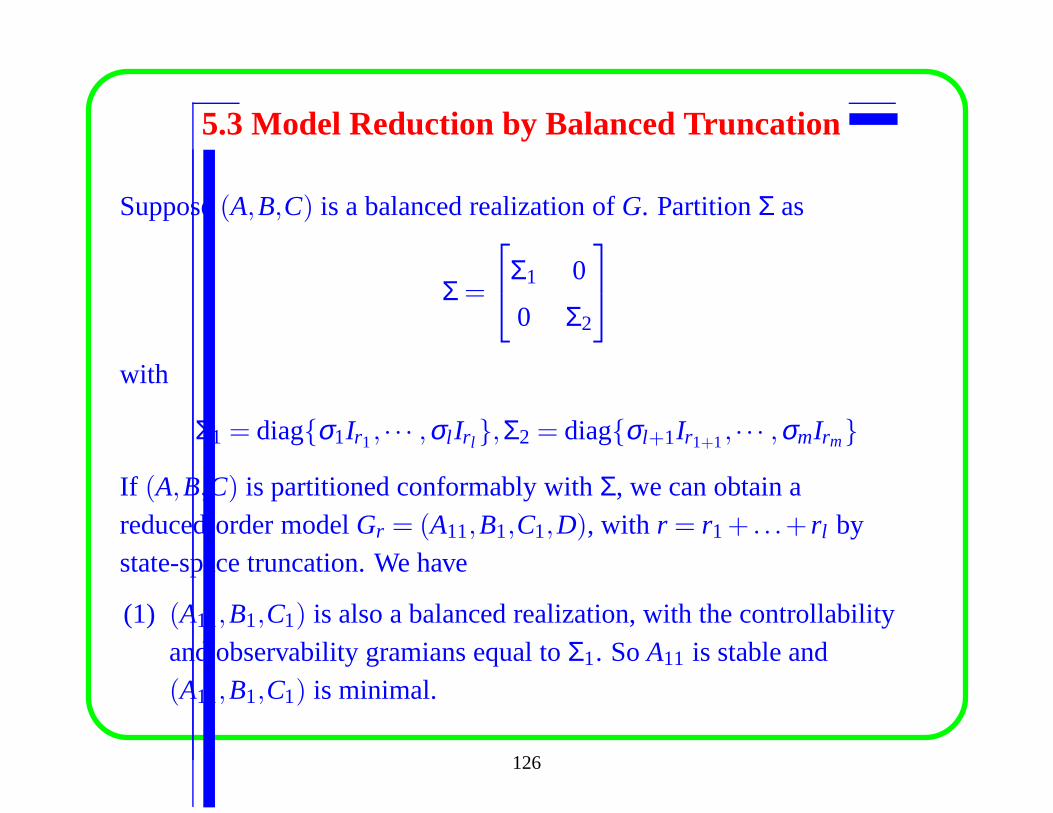
5.3 Model Reduction by Balanced Truncation

Suppose(A,B,C) is a balanced realization ofG. PartitionΣ as

Σ =

Σ1 0

0 Σ2

with

Σ1 = diag{σ1Ir1, · · · ,σl Ir l },Σ2 = diag{σl+1Ir1+1, · · · ,σmIrm}

If (A,B,C) is partitioned conformably withΣ, we can obtain areduced-order modelGr = (A11,B1,C1,D), with r = r1+ . . .+ r l bystate-space truncation. We have

(1) (A11,B1,C1) is also a balanced realization, with the controllabilityand observability gramians equal toΣ1. SoA11 is stable and(A11,B1,C1) is minimal.

126

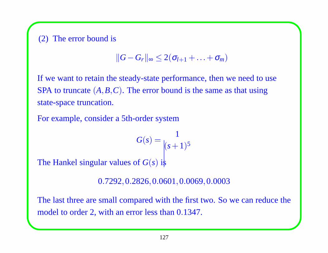
(2) The error bound is

‖G−Gr‖∞ ≤ 2(σl+1+ . . .+σm)

If we want to retain the steady-state performance, then we need to use

SPA to truncate(A,B,C). The error bound is the same as that using

state-space truncation.

For example, consider a 5th-order system

G(s) =1

(s+1)5

The Hankel singular values ofG(s) is

0.7292,0.2826,0.0601,0.0069,0.0003

The last three are small compared with the first two. So we can reduce the

model to order 2, with an error less than 0.1347.

127

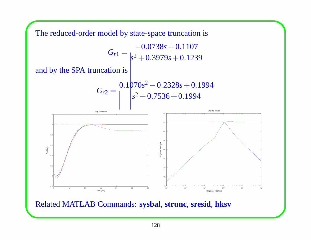
The reduced-order model by state-space truncation is

Gr1 =−0.0738s+0.1107

s2+0.3979s+0.1239

and by the SPA truncation is

Gr2 =0.1070s2−0.2328s+0.1994

s2+0.7536+0.1994

Step Response

Time (sec)

Am

plitu

de

0 5 10 15 20 25 30−0.2

0

0.2

0.4

0.6

0.8

1

1.2

Singular Values

Frequency (rad/sec)

Sin

gula

r V

alue

s (d

B)

10−3

10−2

10−1

100

101

102

−90

−80

−70

−60

−50

−40

−30

−20

−10

Related MATLAB Commands:sysbal, strunc, sresid, hksv

128

5.4 Optimal Model Reduction

The motivation for the balanced truncation method of model reduction

comes from energy transmission arguments. If a high-order modelG

mapsu to y via y= Gu, then the idea is to select a low-order modelGr ,

which mapsu to yr , such that

e= supu∈L2(−∞,0]

(∫ ∞0 (y−yr)

T(y−yr)dt∫ 0−∞ uTudt

)

is small whenu(t) = 0 for t > 0. The quantity can be thought of as the

energy gain from past inputs to future outputs.

The balanced realization method guarantees that the gain issmall. It is

preferred if we can make it minimum. Thus we have the optimal Hankel

norm approximation.

129

Hankel Operators

TheHankel operator of a linear system is the prediction operator thatmaps past inputs to future outputs, assuming the future input is zero.

Suppose the systemG∈ RH∞ is defined by the minimal state-spacerealization

x = Ax+By, x(−∞) = 0

y = Cx+Du

If u∈ L2(−∞,0], then future outputs are determined by

y(t) =∫ 0

−∞CeA(t−τ)Bu(τ)dτ , t > 0

If we setv(t) = u(−t), theny(t) = (ΓGv)(t) for t > 0, whereΓG : L2[0,∞) 7→ L2[0,∞) is the Hankel operator:

(ΓGv)(t) :=∫ ∞

0CeA(t+τ)Bv(τ)dτ

130

Hankel Norm

TheHankel norm of a system is theL2[0,∞) induced norm of its

associated Hankel operator.

‖G‖H = ‖ΓG‖=(

supu∈L2(−∞,0]

( ∫ ∞0 yTydt∫ 0−∞ uTudt

)) 12

For a givenx(0) = x0, we have (c.f. section 13.2)

supu∈L2(−∞,0],x(0)=x0

( ∫ ∞0 yTydt∫ 0−∞ uTudt

)

=xT

0 Qx0

xT0 P−1x0

Thus

‖G‖2H = sup

x0

xT0 Qx0

xT0 P−1x0

= λmax(PQ) = σ21 (largest Hankel singular value)

131

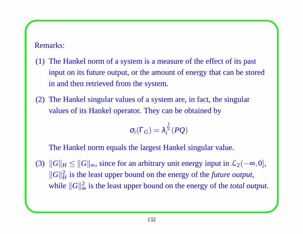
Remarks:

(1) The Hankel norm of a system is a measure of the effect of itspast

input on its future output, or the amount of energy that can bestored

in and then retrieved from the system.

(2) The Hankel singular values of a system are, in fact, the singular

values of its Hankel operator. They can be obtained by

σi(ΓG) = λ12

i (PQ)

The Hankel norm equals the largest Hankel singular value.

(3) ‖G‖H ≤ ‖G‖∞, since for an arbitrary unit energy input inL2(−∞,0],

‖G‖2H is the least upper bound on the energy of thefuture output,

while ‖G‖2∞ is the least upper bound on the energy of thetotal output.

132

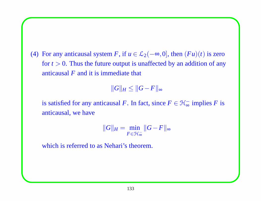
(4) For any anticausal systemF, if u∈ L2(−∞,0], then(Fu)(t) is zero

for t > 0. Thus the future output is unaffected by an addition of any

anticausalF and it is immediate that

‖G‖H ≤ ‖G−F‖∞

is satisfied for any anticausalF. In fact, sinceF ∈H−∞ impliesF is

anticausal, we have

‖G‖H = minF∈H−

∞‖G−F‖∞

which is referred to as Nehari’s theorem.

133

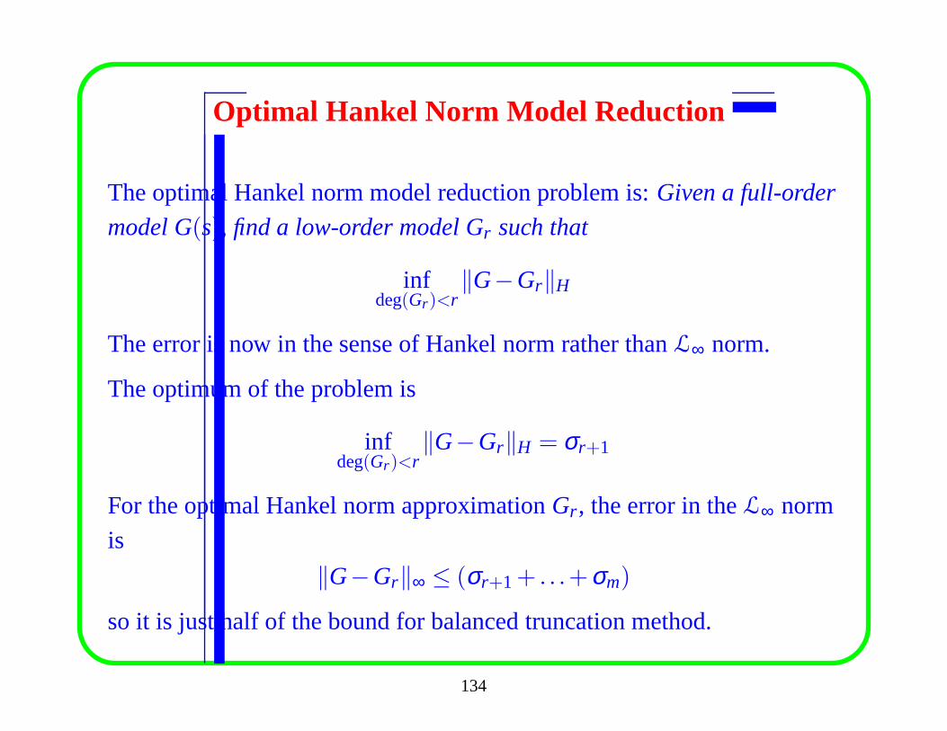
Optimal Hankel Norm Model Reduction

The optimal Hankel norm model reduction problem is:Given a full-order

model G(s), find a low-order model Gr such that

infdeg(Gr )<r

‖G−Gr‖H

The error is now in the sense of Hankel norm rather thanL∞ norm.

The optimum of the problem is

infdeg(Gr )<r

‖G−Gr‖H = σr+1

For the optimal Hankel norm approximationGr , the error in theL∞ norm

is

‖G−Gr‖∞ ≤ (σr+1+ . . .+σm)

so it is just half of the bound for balanced truncation method.

134

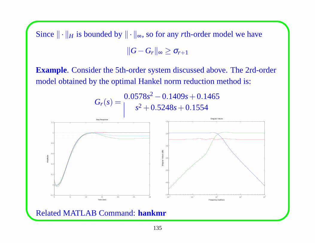
Since‖ · ‖H is bounded by‖ · ‖∞, so for anyrth-order model we have

‖G−Gr‖∞ ≥ σr+1

Example. Consider the 5th-order system discussed above. The 2rd-ordermodel obtained by the optimal Hankel norm reduction method is:

Gr(s) =0.0578s2−0.1409s+0.1465

s2+0.5248s+0.1554Step Response

Time (sec)

Am

plitu

de

0 5 10 15 20 25 30−0.2

0

0.2

0.4

0.6

0.8

1

1.2

Singular Values

Frequency (rad/sec)

Sin

gula

r V

alue

s (d

B)

10−2

10−1

100

101

102

−70

−60

−50

−40

−30

−20

−10

Related MATLAB Command:hankmr

135

5.5 Coprime Factorization Reduction

Another method for model/controller reduction is to use thecoprime

factorization of a model. Suppose an nlcf of a plantG is G= M−1N.

If we reduce the ‘numerator’ and the ‘denominator’ of the model

simultaneously tor-th order,Mr , Nr , thenGr := M−1r Nr appears to be a

‘close’ approximation toG.

To show that, let

D(s) :=

M

N

, Dr(s) :=

Mr

Nr

Consider the approximation ofD(s) by Dr(s). Suppose there exists a

Q(s) ∈ RH∞ such that

Dr(s) = D(s)Q(s)

136

then the approximation error‖D(s)−Dr(s)‖∞ < γ means∥∥∥∥∥∥

M

N

−

M

N

Q

∥∥∥∥∥∥

∞

< γ

soGr belongs to

{(M+∆M)−1(N+∆N) : ‖[ ∆M ∆N ]‖∞ ≤ γ}

Thus if γ is small, thenGr is close toG in the coprime factorization sense

(gap metric). Thus we can use normalized coprime factorization to

perform a model reduction, where the approximation ofD(s) by Dr(s)

can be done either using balanced truncation or optimal Hankel reduction

method.

137

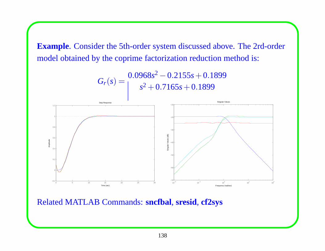
Example. Consider the 5th-order system discussed above. The 2rd-order

model obtained by the coprime factorization reduction method is:

Gr(s) =0.0968s2−0.2155s+0.1899

s2+0.7165s+0.1899

Step Response

Time (sec)

Am

plitu

de

0 5 10 15 20 25 30−0.2

0

0.2

0.4

0.6

0.8

1

1.2

Singular Values

Frequency (rad/sec)

Sin

gula

r V

alue

s (d

B)

10−2

10−1

100

101

102

−70

−60

−50

−40

−30

−20

−10

Related MATLAB Commands:sncfbal, sresid, cf2sys

138

Summary

• The balanced truncation method and the optimal Hankel method are

not applicable to unstable models. If a model contains unstable poles,

we need first decompose it into a stable part and an unstable part. The

order can only be reduced for the stable part. The final reduced-order

model is then obtained by adding the unstable part and the

reduced-order stable part.

• The coprime factorization reduction method can be applied to both

stable and unstable models, so there is no need to have a

decomposition first.

• The coprime factorization reduction method makes sense in the gap

metric. It does not guarantee a bound for the error in the infinity

norm.

139

5.6 PID Approximation

About 90% of industrial controllers are of PID-type. So it isuseful if the

high-order controllers can be reduced to PID control structure. Two

methods can be used to make the approximation:

1. In the state-space domain.

2. In the frequency-domain.

140

PID Approximation in Time-Domain

Consider a controllerK(s), given by a state-space realization of the form

x= Akx+Bky

u=Ckx+Dky

Find a similarity transformationT such that

TAkT−1 =

0 0

0 A2

This transformation can be computed using the eigenvalue decompositionof Ak. With thisT, the new state-space realization is given by

˙x= Akx+ Bky,

u= Ckx+ Dky,

141

with Ak = TAkT−1, Dk = Dk, and

Ck =CkT−1 =

[

C1 C2

]

, Bk = TBk =

B1

B2

A PID approximation of the form

KPID(s) = Kp+Ki/s+Kds

can now be obtained by truncating the Maclaurin expansion ofthecontroller with respect to the variables:

K(s) =[

C1 C2

]

sI 0

0 sI−A2

−1

B1

B2

+Dk

= C1B1s +(Dk−C2A−1

2 B2)−C2A−22 B2s+ · · · ,

So we have

Kp = Dk−C2A−12 B2, Ki =C1B1, Kd =−C2A−2

2 B2.

142

It is then clear that the resulting PID controller achieves good

approximation at low frequencies, especially the integralaction, so we

can expect that the resulting PID controller will retain thedisturbance

rejection performance of the high-order controller.

The following steps need to be considered after the reduction procedure:

1. Due to the minimum-phase requirement of a PID controller,the signs

of the proportional gain, the integral gain and the differentiator

should be the same. So if the corresponding elements ofKp, Ki and

Kd do not have the same sign, then we need to discard the term that

has the opposite sign with the element inKi , which is the most

important term.

143

2. The derivative action should be taken with care. We find that a PID

approximation with ideal differentiators sometimes destabilizes a

process even though the original high-order controller works well.

This seldom happens for single-loop processes, but it is quite

common for multivariable processes. We believe the reason is that

the phase information of the original controller is lost when using an

ideal differentiator. Thus, a filter of the form1αs+1 should be used for

the differentiator.

144

PID Approximation in Frequency Domain

The standard procedure for obtaining PID parameters from IMCcontrollers is to expand the final controller into MacLaurian series and getthe coefficients of the first three terms. However, the procedure is notconvenient and sometimes not sufficient.

One-point Approximation

A new method to approximate any high-order controller with PID in thefrequency domain with one point approximation goes as follows:

1. Given any controllerK(s), get a frequency range of interest, computethe frequency response ofK(s).

2. Find the frequencyωz such that the magnitude ofK( jω) achieves itsminimum value.

145

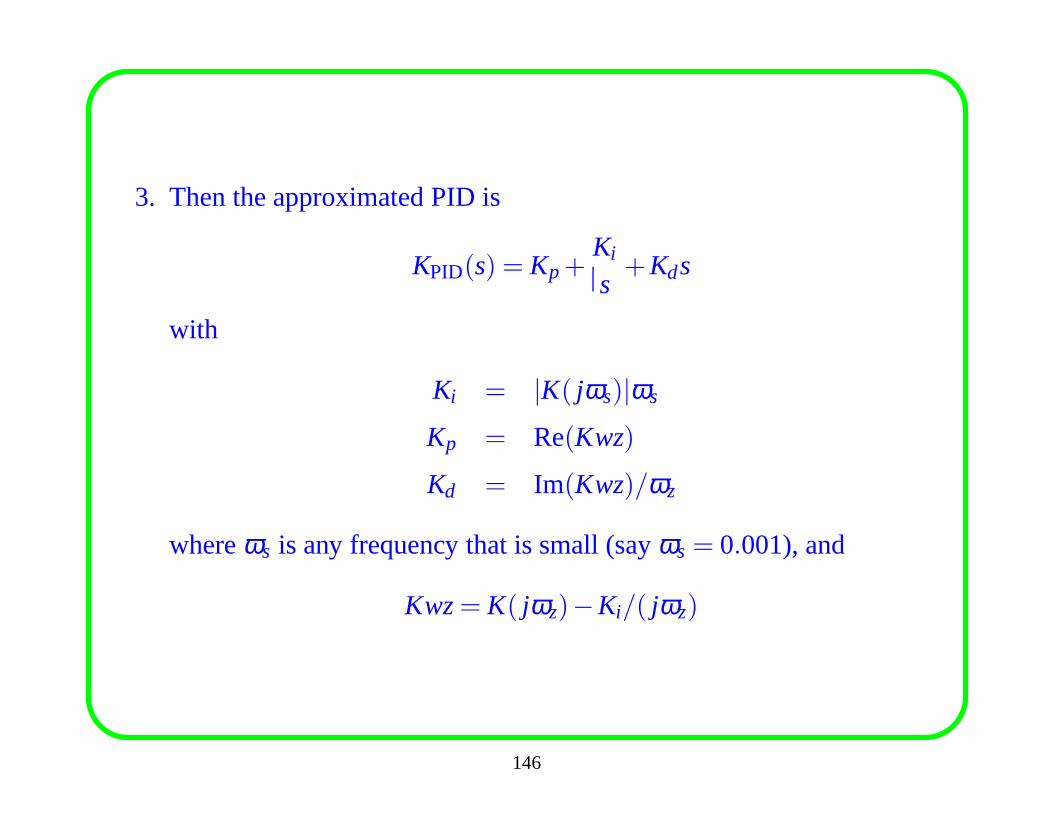
3. Then the approximated PID is

KPID(s) = Kp+Ki

s+Kds

with

Ki = |K( jωs)|ωs

Kp = Re(Kwz)

Kd = Im(Kwz)/ωz

whereωs is any frequency that is small (sayωs = 0.001), and

Kwz= K( jωz)−Ki/( jωz)

146

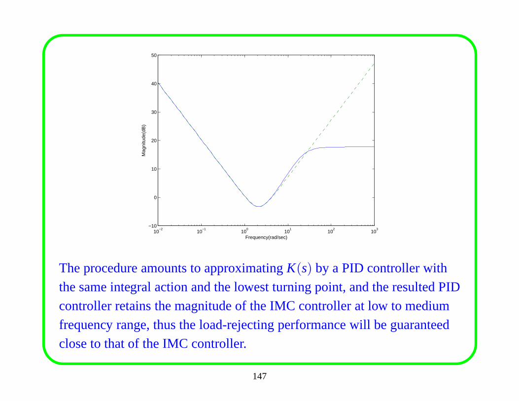
10−2

10−1

100

101

102

103

−10

0

10

20

30

40

50

Frequency(rad/sec)

Mag

nitu

de(d

B)

The procedure amounts to approximatingK(s) by a PID controller withthe same integral action and the lowest turning point, and the resulted PIDcontroller retains the magnitude of the IMC controller at low to mediumfrequency range, thus the load-rejecting performance willbe guaranteedclose to that of the IMC controller.

147

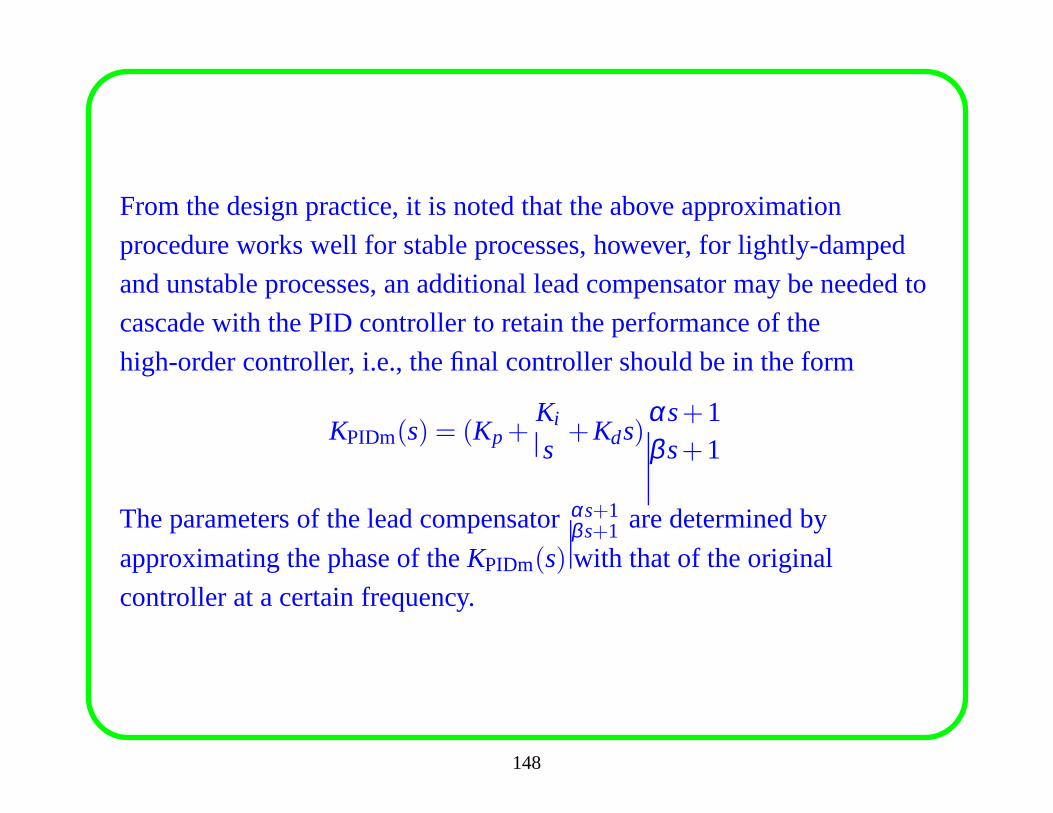
From the design practice, it is noted that the above approximation

procedure works well for stable processes, however, for lightly-damped

and unstable processes, an additional lead compensator maybe needed to

cascade with the PID controller to retain the performance ofthe

high-order controller, i.e., the final controller should bein the form

KPIDm(s) = (Kp+Ki

s+Kds)

αs+1βs+1

The parameters of the lead compensatorαs+1βs+1 are determined by

approximating the phase of theKPIDm(s) with that of the original

controller at a certain frequency.

148

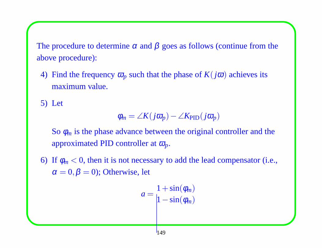
The procedure to determineα andβ goes as follows (continue from the

above procedure):

4) Find the frequencyωp such that the phase ofK( jω) achieves its

maximum value.

5) Let

φm = ∠K( jωp)−∠KPID( jωp)

Soφm is the phase advance between the original controller and the

approximated PID controller atωp.

6) If φm < 0, then it is not necessary to add the lead compensator (i.e.,

α = 0,β = 0); Otherwise, let

a=1+sin(φm)

1−sin(φm)

149

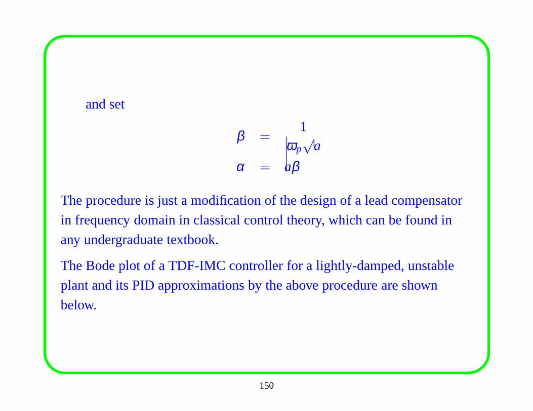
and set

β =1

ωp√

a

α = aβ

The procedure is just a modification of the design of a lead compensator

in frequency domain in classical control theory, which can be found in

any undergraduate textbook.

The Bode plot of a TDF-IMC controller for a lightly-damped, unstable

plant and its PID approximations by the above procedure are shown

below.

150

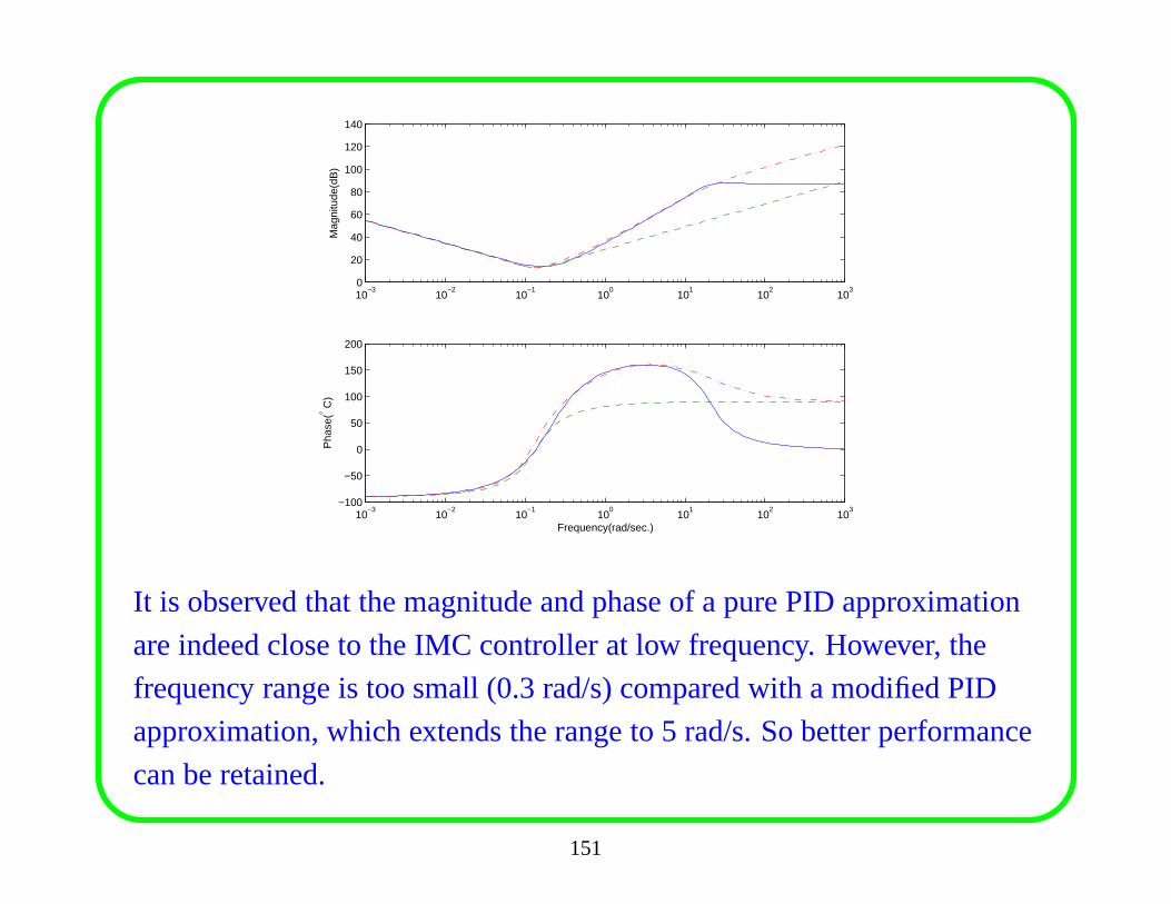
10−3

10−2

10−1

100

101

102

103

0

20

40

60

80

100

120

140

Mag

nitu

de(d

B)

10−3

10−2

10−1

100

101

102

103

−100

−50

0

50

100

150

200

Frequency(rad/sec.)

Pha

se(° C

)

It is observed that the magnitude and phase of a pure PID approximation

are indeed close to the IMC controller at low frequency. However, the

frequency range is too small (0.3 rad/s) compared with a modified PID

approximation, which extends the range to 5 rad/s. So betterperformance

can be retained.

151

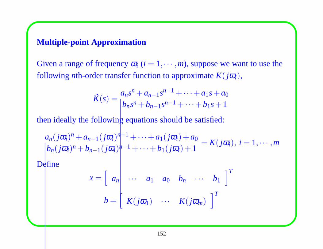
Multiple-point Approximation

Given a range of frequencyωi (i = 1, · · · ,m), suppose we want to use the

following nth-order transfer function to approximateK( jωi),

K(s) =ansn+an−1sn−1+ · · ·+a1s+a0

bnsn+bn−1sn−1+ · · ·+b1s+1

then ideally the following equations should be satisfied:

an( jωi)n+an−1( jωi)

n−1+ · · ·+a1( jωi)+a0

bn( jωi)n+bn−1( jωi)n−1+ · · ·+b1( jωi)+1= K( jωi), i = 1, · · · ,m

Define

x=[

an · · · a1 a0 bn · · · b1

]T

b=[

K( jω1) · · · K( jωm)]T

152

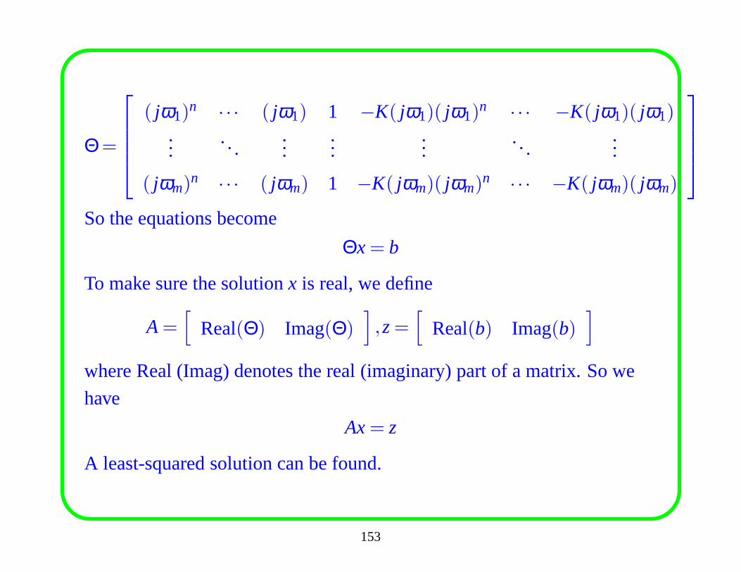
Θ=

( jω1)n · · · ( jω1) 1 −K( jω1)( jω1)

n · · · −K( jω1)( jω1)...

......

......

......

( jωm)n · · · ( jωm) 1 −K( jωm)( jωm)

n · · · −K( jωm)( jωm)

So the equations become

Θx= b

To make sure the solutionx is real, we define

A=[

Real(Θ) Imag(Θ)]

,z=[

Real(b) Imag(b)]

where Real (Imag) denotes the real (imaginary) part of a matrix. So we

have

Ax= z

A least-squared solution can be found.

153

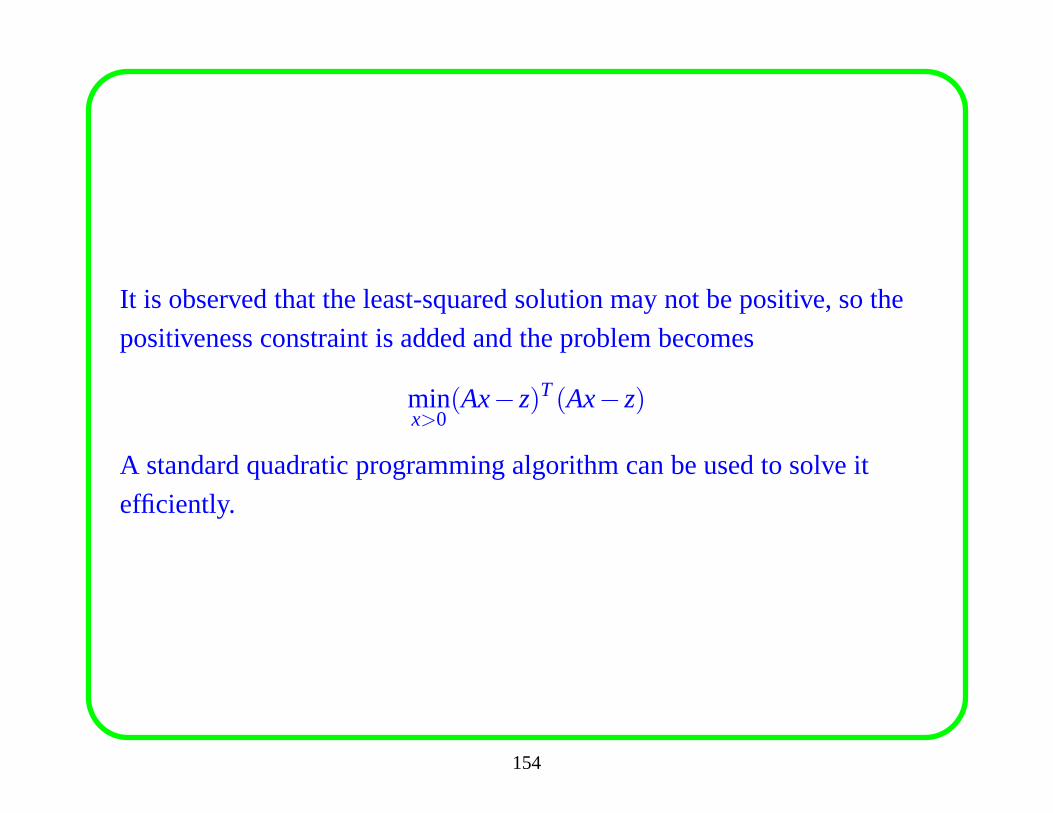
It is observed that the least-squared solution may not be positive, so the

positiveness constraint is added and the problem becomes

minx>0

(Ax−z)T(Ax−z)

A standard quadratic programming algorithm can be used to solve it

efficiently.

154

Chapter 6. Robustness Measure

In this chapter a simple method will be proposed to measure system

robustness and performance. It is shown that the method can be applied to

various industrial processes, no matter they are stable, integrating, or

unstable; single-loop, cascade, or multivariable.

155

6.1 Classical Robustness Measures

6.1.1 Robustness Measure in terms ofMs

Gain and phase margins are generally used in the classical control theory

to measure system robustness for a single-input-single-output (SISO)

process. If the open-loop transfer function of a linear system is

L(s) := G(s)K(s), then the gain margin (GM) is

GM =1

|L( jωp)|

whereωp is the phase crossover frequency, and the phase margin (PM) is

PM= ∠L( jωg)−180◦

whereωg is the gain crossover frequency.

156

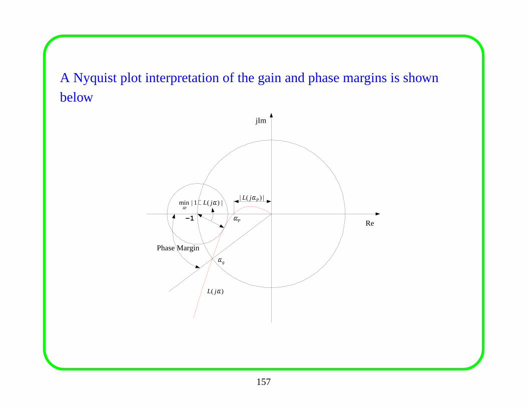
A Nyquist plot interpretation of the gain and phase margins is shown

below

-1

Phase Margin

gω

Pω

|)(| PjL ω

)( ωjL

|)(1|min ωω

jL+

Re

jIm

157

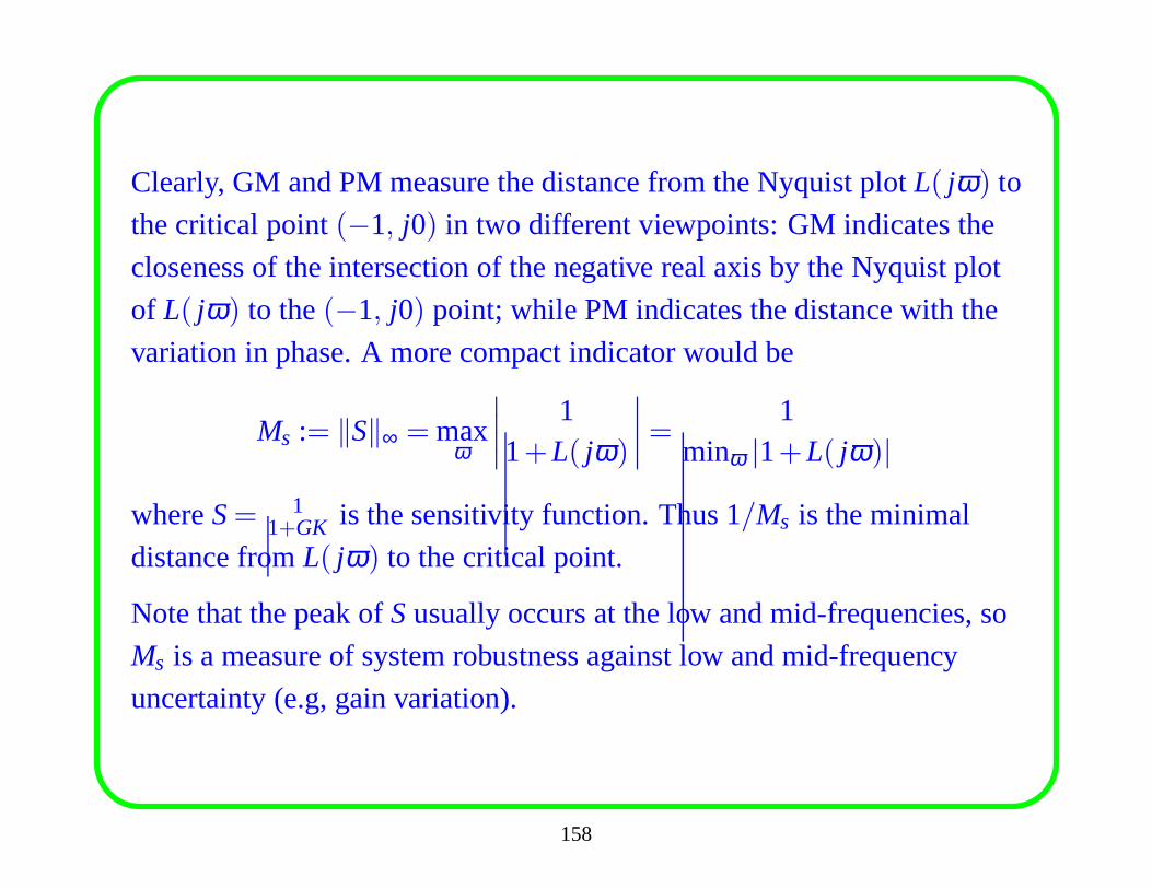
Clearly, GM and PM measure the distance from the Nyquist plotL( jω) to

the critical point(−1, j0) in two different viewpoints: GM indicates the

closeness of the intersection of the negative real axis by the Nyquist plot

of L( jω) to the(−1, j0) point; while PM indicates the distance with the

variation in phase. A more compact indicator would be

Ms := ‖S‖∞ = maxω

∣∣∣∣

11+L( jω)

∣∣∣∣=

1minω |1+L( jω)|

whereS= 11+GK is the sensitivity function. Thus 1/Ms is the minimal

distance fromL( jω) to the critical point.

Note that the peak ofSusually occurs at the low and mid-frequencies, so

Ms is a measure of system robustness against low and mid-frequency

uncertainty (e.g, gain variation).

158

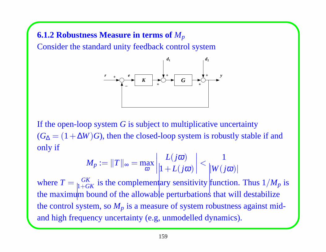
6.1.2 Robustness Measure in terms ofMp

Consider the standard unity feedback control system

K Gr y

_

e

d1

+

d2

+

+

+

+

If the open-loop systemG is subject to multiplicative uncertainty(G∆ = (1+∆W)G), then the closed-loop system is robustly stable if andonly if

Mp := ‖T‖∞ = maxω

∣∣∣∣

L( jω)

1+L( jω)

∣∣∣∣<

1|W( jω)|

whereT = GK1+GK is the complementary sensitivity function. Thus 1/Mp is

the maximum bound of the allowable perturbations that will destabilizethe control system, soMp is a measure of system robustness against mid-and high frequency uncertainty (e.g, unmodelled dynamics).

159

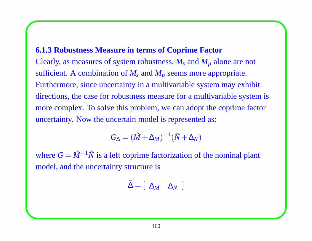
6.1.3 Robustness Measure in terms of Coprime FactorClearly, as measures of system robustness,Ms andMp alone are not

sufficient. A combination ofMs andMp seems more appropriate.

Furthermore, since uncertainty in a multivariable system may exhibit

directions, the case for robustness measure for a multivariable system is

more complex. To solve this problem, we can adopt the coprimefactor

uncertainty. Now the uncertain model is represented as:

G∆ = (M+∆M)−1(N+∆N)

whereG= M−1N is a left coprime factorization of the nominal plant

model, and the uncertainty structure is

∆ = [ ∆M ∆N ]

160

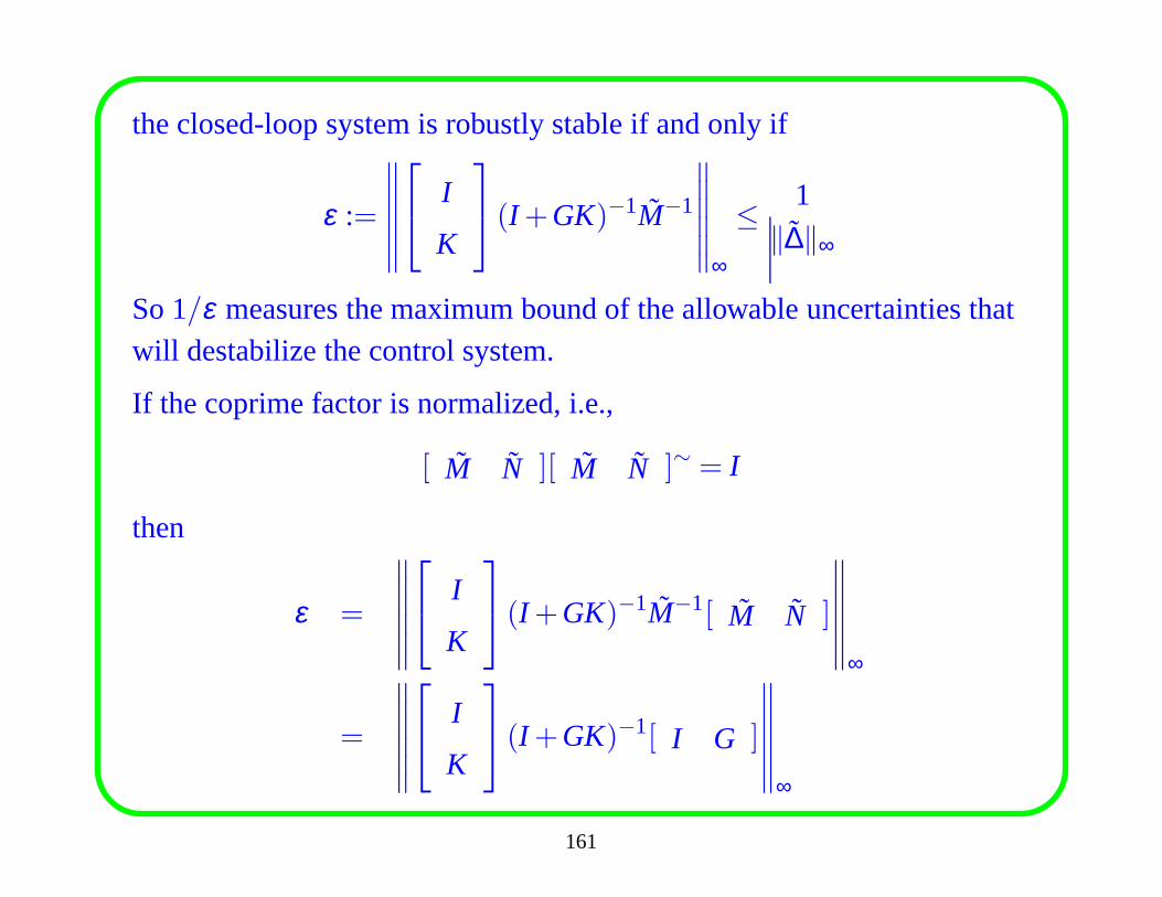
the closed-loop system is robustly stable if and only if

ε :=

∥∥∥∥∥∥

I

K

(I +GK)−1M−1

∥∥∥∥∥∥

∞

≤ 1

‖∆‖∞

So 1/ε measures the maximum bound of the allowable uncertainties thatwill destabilize the control system.

If the coprime factor is normalized, i.e.,

[ M N ][ M N ]∼ = I

then

ε =

∥∥∥∥∥∥

I

K

(I +GK)−1M−1[ M N ]

∥∥∥∥∥∥

∞

=

∥∥∥∥∥∥

I

K

(I +GK)−1[ I G ]

∥∥∥∥∥∥

∞

161

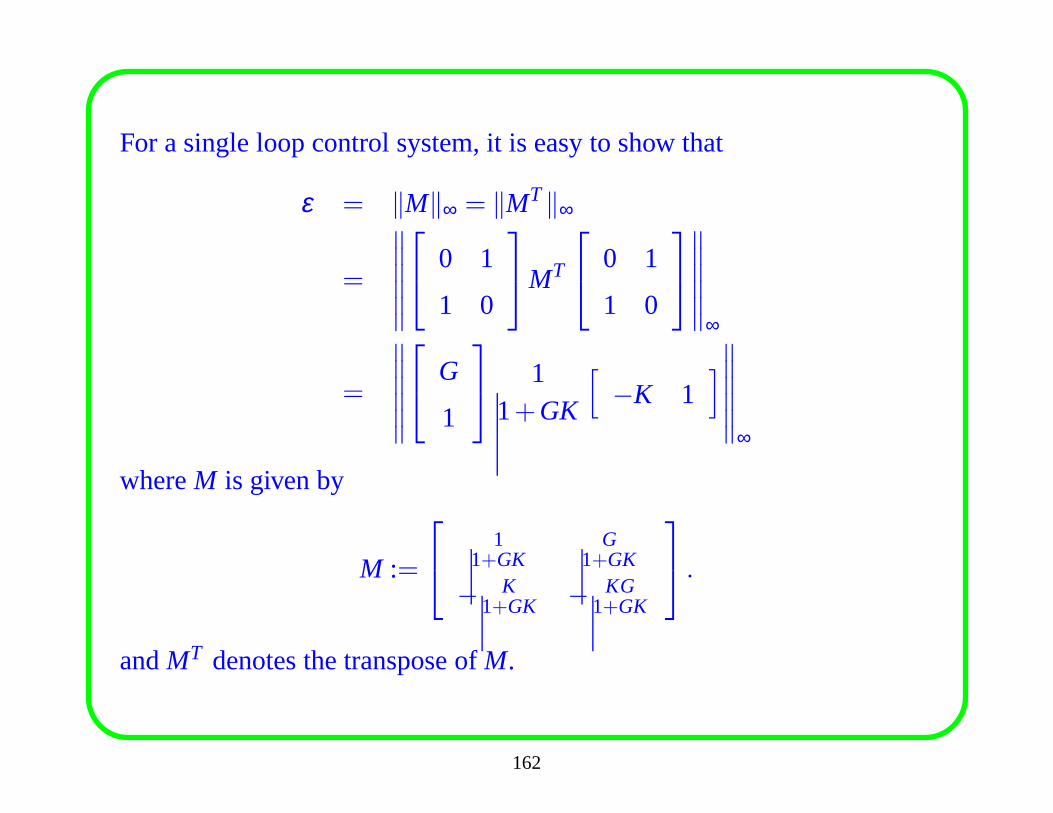
For a single loop control system, it is easy to show that

ε = ‖M‖∞ = ‖MT‖∞

=

∥∥∥∥∥∥

0 1

1 0

MT

0 1

1 0

∥∥∥∥∥∥

∞

=

∥∥∥∥∥∥

G

1

1

1+GK

[

−K 1]

∥∥∥∥∥∥

∞

whereM is given by

M :=

11+GK

G1+GK

− K1+GK − KG

1+GK

.

andMT denotes the transpose ofM.

162

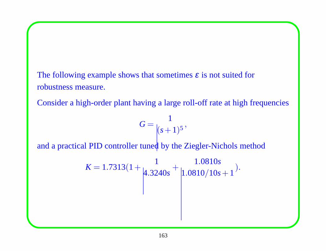
The following example shows that sometimesε is not suited for

robustness measure.

Consider a high-order plant having a large roll-off rate at high frequencies

G=1

(s+1)5 ,

and a practical PID controller tuned by the Ziegler-Nicholsmethod

K = 1.7313(1+1

4.3240s+

1.0810s1.0810/10s+1

).

163

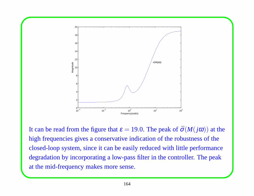
10−2

10−1

100

101

102

0

2

4

6

8

10

12

14

16

18

20

Frequency(rad/s)

Mag

nitu

de

σ(M(jω))

It can be read from the figure thatε = 19.0. The peak ofσ(M( jω)) at the

high frequencies gives a conservative indication of the robustness of the

closed-loop system, since it can be easily reduced with little performance

degradation by incorporating a low-pass filter in the controller. The peak

at the mid-frequency makes more sense.

164

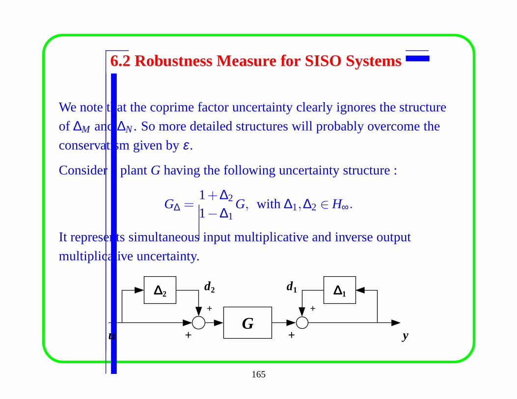
6.2 Robustness Measure for SISO Systems

We note that the coprime factor uncertainty clearly ignoresthe structure

of ∆M and∆N. So more detailed structures will probably overcome the

conservatism given byε .

Consider a plantG having the following uncertainty structure :

G∆ =1+∆2

1−∆1G, with ∆1,∆2 ∈ H∞.

It represents simultaneous input multiplicative and inverse output

multiplicative uncertainty.

∆∆∆∆2

G

∆∆∆∆1

+ +

d2 d1

u y+ +

165

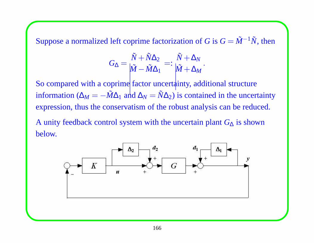
Suppose a normalized left coprime factorization ofG is G= M−1N, then

G∆ =N+ N∆2

M− M∆1=:

N+∆N

M+∆M.

So compared with a coprime factor uncertainty, additional structure

information (∆M =−M∆1 and∆N = N∆2) is contained in the uncertainty

expression, thus the conservatism of the robust analysis can be reduced.

A unity feedback control system with the uncertain plantG∆ is shown

below.

166

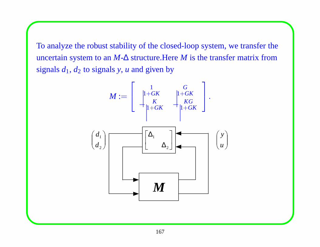
To analyze the robust stability of the closed-loop system, we transfer the

uncertain system to anM-∆ structure.HereM is the transfer matrix from

signalsd1, d2 to signalsy, u and given by

M :=

11+GK

G1+GK

− K1+GK − KG

1+GK

.

M

∆∆

2

1

2

1

d

d

u

y

167

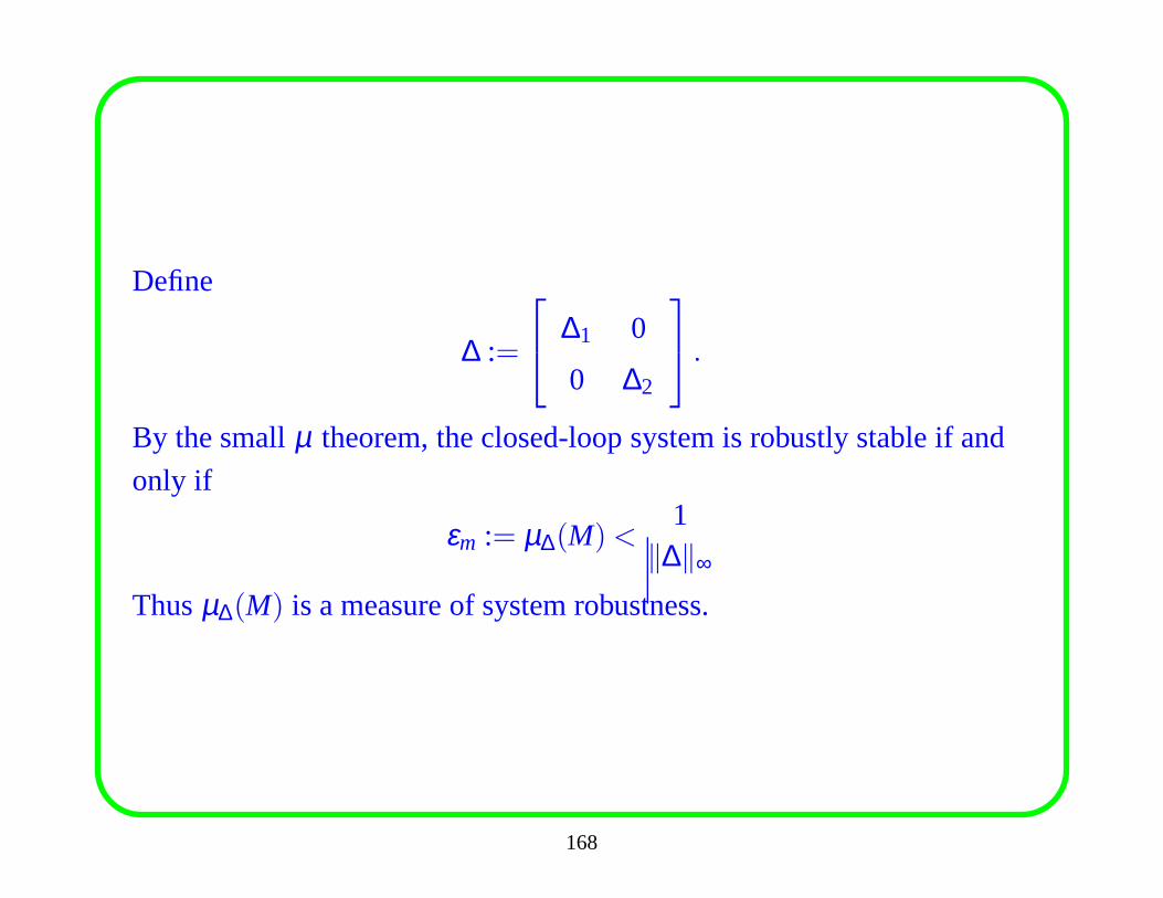
Define

∆ :=

∆1 0

0 ∆2

.

By the smallµ theorem, the closed-loop system is robustly stable if and

only if

εm := µ∆(M)<1

‖∆‖∞

Thusµ∆(M) is a measure of system robustness.

168

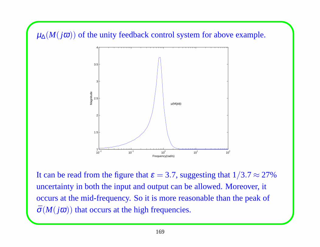
µ∆(M( jω)) of the unity feedback control system for above example.

10−2

10−1

100

101

102

1

1.5

2

2.5

3

3.5

4

Frequency(rad/s)

Mag

nitu

de

µ(M(jω))

It can be read from the figure thatε = 3.7, suggesting that 1/3.7≈ 27%uncertainty in both the input and output can be allowed. Moreover, itoccurs at the mid-frequency. So it is more reasonable than the peak ofσ(M( jω)) that occurs at the high frequencies.

169

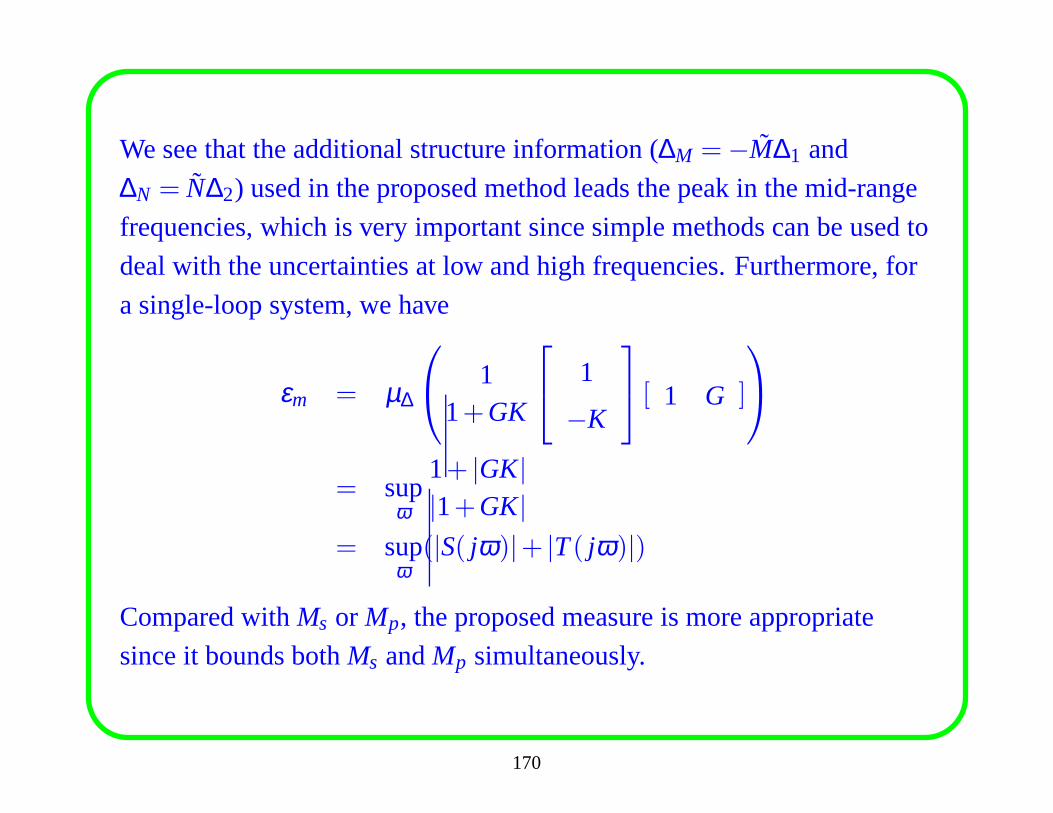
We see that the additional structure information (∆M =−M∆1 and

∆N = N∆2) used in the proposed method leads the peak in the mid-range

frequencies, which is very important since simple methods can be used to

deal with the uncertainties at low and high frequencies. Furthermore, for

a single-loop system, we have

εm = µ∆

1

1+GK

1

−K

[ 1 G ]

= supω

1+ |GK||1+GK|

= supω(|S( jω)|+ |T( jω)|)

Compared withMs or Mp, the proposed measure is more appropriate

since it bounds bothMs andMp simultaneously.

170

Application: Comparison of PID tuning formulas

Evaluation of various PID design or tuning methods found in the

literature can be done by using some performance criteria. However,

since a specific method might be effective for a specific plantmodel, it is

hazardous to draw general conclusions on which method is thebest (in

fact, no best at all). What we can conclude is that some methods show

better performance in disturbance rejection and/or robustness than other

methods.

In this section, we will apply the criteria proposed in the previous section

to analyze several PID tuning techniques found in the literature.

171

The process model is first-order with deadtime (FOPDT)

G(s) =k

Ts+1e−τs.

The following PID tuning formulas are considered:

1. Ziegler-Nichols (Z-N) method

2. Internal model control (IMC) method.

3. Gain-phase margin (G-P) method.

4. Optimum integral error for load disturbance (IAE-load, ITAE-load,

ISE-load, ISTE-load), and for setpoint change (IAE-setpoint,

ITAE-setpoint, ISE-setpoint, ISTE-setpoint) methods.

172

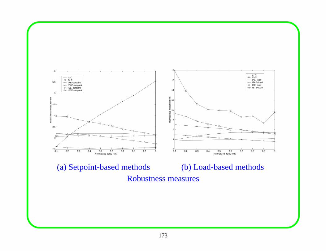
0.1 0.2 0.3 0.4 0.5 0.6 0.7 0.8 0.9 12.5

3

3.5

4

4.5

5

5.5

6

Normalized delay (τ/T)

Rob

ustn

ess

mea

sure

men

t

IMCG−PIAE−setpointITAE−setpointISE−setpointISTE−setpoint

0.1 0.2 0.3 0.4 0.5 0.6 0.7 0.8 0.9 12

4

6

8

10

12

14

16

18

Normalized delay (τ/T)

Rob

ustn

ess

mea

sure

men

t

Z−NC−CIAE−loadITAE−loadISE−loadISTE−load

(a) Setpoint-based methods (b) Load-based methodsRobustness measures

173

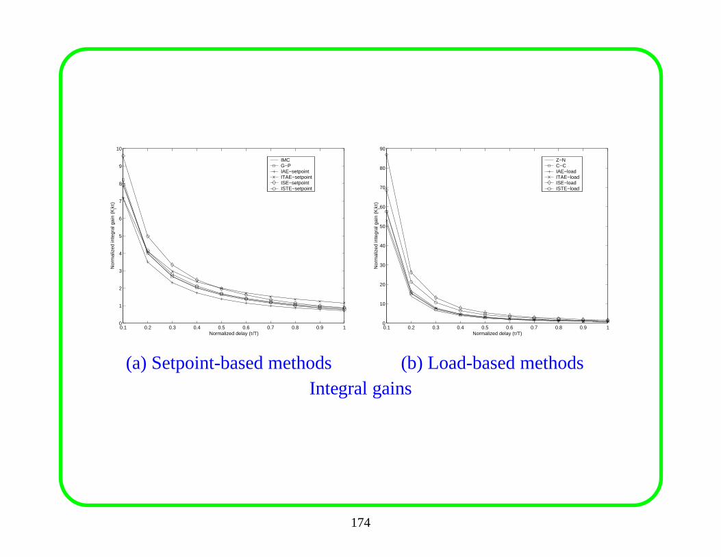
0.1 0.2 0.3 0.4 0.5 0.6 0.7 0.8 0.9 10

1

2

3

4

5

6

7

8

9

10

Normalized delay (τ/T)

Nor

mal

ized

inte

gral

gai

n (K

ikτ)

IMCG−PIAE−setpointITAE−setpointISE−setpointISTE−setpoint

0.1 0.2 0.3 0.4 0.5 0.6 0.7 0.8 0.9 10

10

20

30

40

50

60

70

80

90

Normalized delay (τ/T)

Nor

mal

ized

inte

gral

gai

n (K

ikτ)

Z−NC−CIAE−loadITAE−loadISE−loadISTE−load

(a) Setpoint-based methods (b) Load-based methodsIntegral gains

174

The following can be observed:

1. IMC and G-P methods can be regarded as setpoint-based tuning

methods, since the integral gains of the PID controllers tuned by the

two methods are close to those of the setpoint-based optimum

integral error methods. Similarly Z-N and C-C methods can be

regarded as load-based tuning methods.

2. The robustness measures of the setpoint-based methods are less than

4 except the ITAE-setpoint method for processes with large delay;

while those for the load-based methods are greater than 4, except the

Z-N method for processes with small delay and the ITAE-load

method for processes with large delay. So the PID controllers tuned

by the setpoint-based methods are usually more robust than those

tuned by the load-based methods.

175

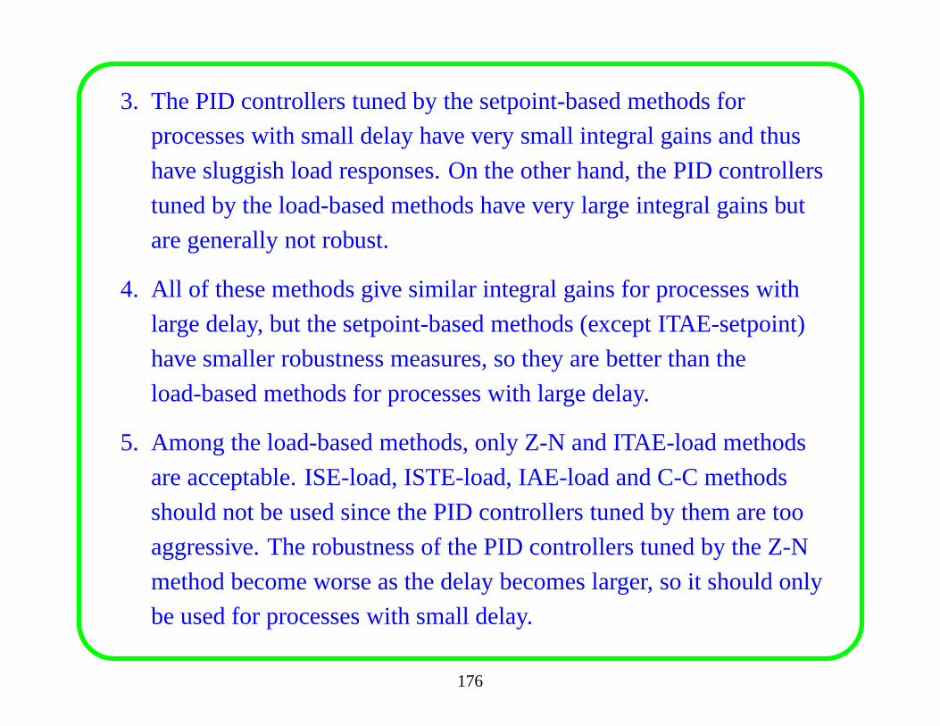
3. The PID controllers tuned by the setpoint-based methods for

processes with small delay have very small integral gains and thus

have sluggish load responses. On the other hand, the PID controllers

tuned by the load-based methods have very large integral gains but

are generally not robust.

4. All of these methods give similar integral gains for processes with

large delay, but the setpoint-based methods (except ITAE-setpoint)

have smaller robustness measures, so they are better than the

load-based methods for processes with large delay.

5. Among the load-based methods, only Z-N and ITAE-load methods

are acceptable. ISE-load, ISTE-load, IAE-load and C-C methods

should not be used since the PID controllers tuned by them aretoo

aggressive. The robustness of the PID controllers tuned by the Z-N

method become worse as the delay becomes larger, so it shouldonly

be used for processes with small delay.

176

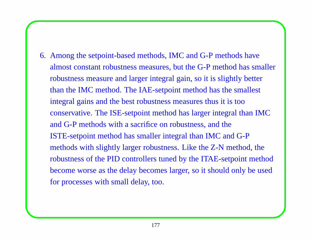
6. Among the setpoint-based methods, IMC and G-P methods have

almost constant robustness measures, but the G-P method hassmaller

robustness measure and larger integral gain, so it is slightly better

than the IMC method. The IAE-setpoint method has the smallest

integral gains and the best robustness measures thus it is too

conservative. The ISE-setpoint method has larger integralthan IMC

and G-P methods with a sacrifice on robustness, and the

ISTE-setpoint method has smaller integral than IMC and G-P

methods with slightly larger robustness. Like the Z-N method, the

robustness of the PID controllers tuned by the ITAE-setpoint method

become worse as the delay becomes larger, so it should only beused

for processes with small delay, too.

177

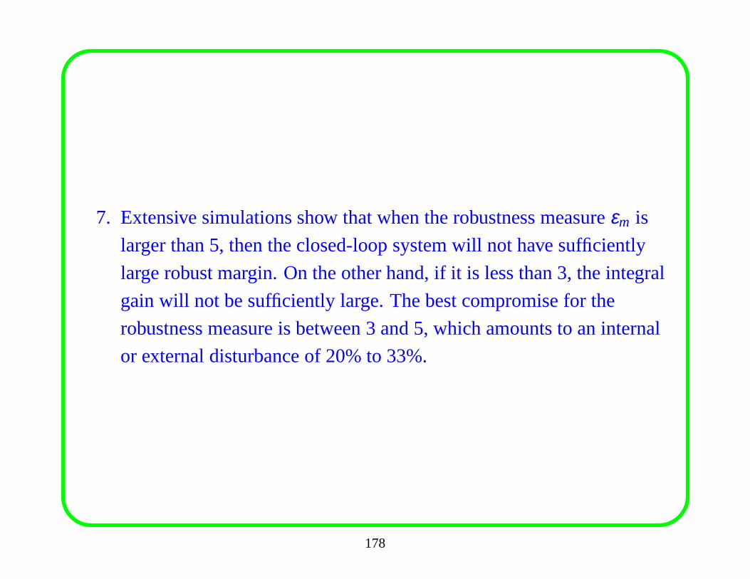
7. Extensive simulations show that when the robustness measureεm is

larger than 5, then the closed-loop system will not have sufficiently

large robust margin. On the other hand, if it is less than 3, the integral

gain will not be sufficiently large. The best compromise for the

robustness measure is between 3 and 5, which amounts to an internal

or external disturbance of 20% to 33%.

178

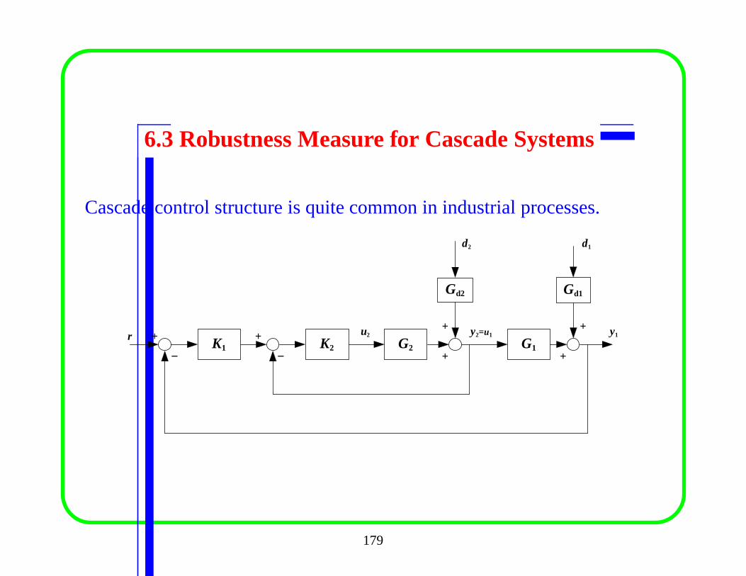
6.3 Robustness Measure for Cascade Systems

Cascade control structure is quite common in industrial processes.

K2 G2r y2=u1

_

Gd2

y1

d2

+

G1K1

Gd1

d1

u2+ +

+ +

+

_

179

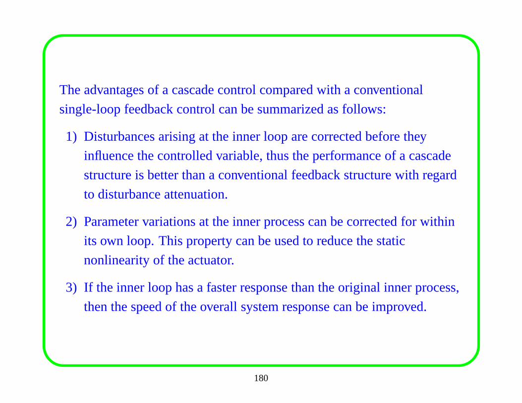
The advantages of a cascade control compared with a conventional

single-loop feedback control can be summarized as follows:

1) Disturbances arising at the inner loop are corrected before they

influence the controlled variable, thus the performance of acascade

structure is better than a conventional feedback structurewith regard

to disturbance attenuation.

2) Parameter variations at the inner process can be corrected for within

its own loop. This property can be used to reduce the static

nonlinearity of the actuator.

3) If the inner loop has a faster response than the original inner process,

then the speed of the overall system response can be improved.

180

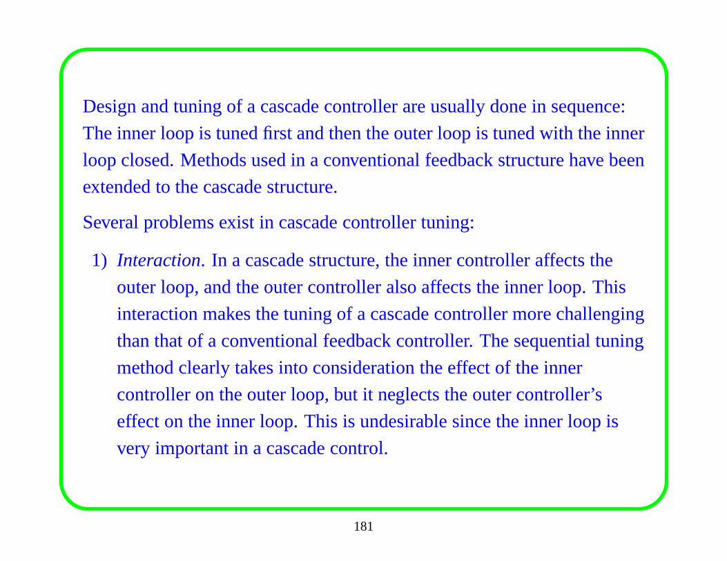
Design and tuning of a cascade controller are usually done insequence:

The inner loop is tuned first and then the outer loop is tuned with the inner

loop closed. Methods used in a conventional feedback structure have been

extended to the cascade structure.

Several problems exist in cascade controller tuning:

1) Interaction. In a cascade structure, the inner controller affects the

outer loop, and the outer controller also affects the inner loop. This

interaction makes the tuning of a cascade controller more challenging

than that of a conventional feedback controller. The sequential tuning

method clearly takes into consideration the effect of the inner

controller on the outer loop, but it neglects the outer controller’s

effect on the inner loop. This is undesirable since the innerloop is

very important in a cascade control.

181

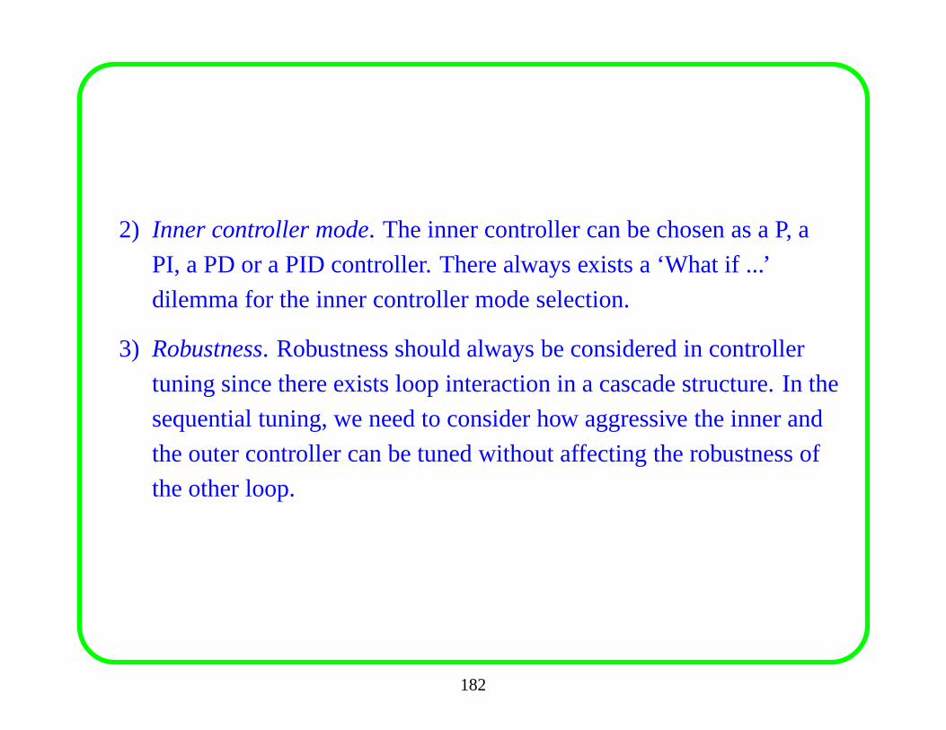
2) Inner controller mode. The inner controller can be chosen as a P, a

PI, a PD or a PID controller. There always exists a ‘What if ...’

dilemma for the inner controller mode selection.

3) Robustness. Robustness should always be considered in controller

tuning since there exists loop interaction in a cascade structure. In the

sequential tuning, we need to consider how aggressive the inner and

the outer controller can be tuned without affecting the robustness of

the other loop.

182

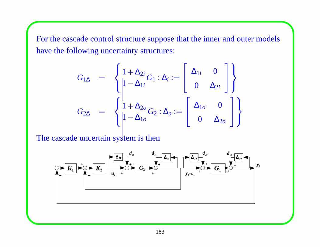
For the cascade control structure suppose that the inner andouter models

have the following uncertainty structures:

G1∆ =

1+∆2i

1−∆1iG1 : ∆i :=

∆1i 0

0 ∆2i

G2∆ =

1+∆2o

1−∆1oG2 : ∆o :=

∆1o 0

0 ∆2o

The cascade uncertain system is then

K2

∆∆∆∆ 2i

G2

∆∆∆∆ 1i

+ +

_

d2i d1i

y1

∆∆∆∆ 2o

G1

∆∆∆∆ 1o

+ +

d2o d1o

K1_ y2=u1u2

+

+ ++ +

183

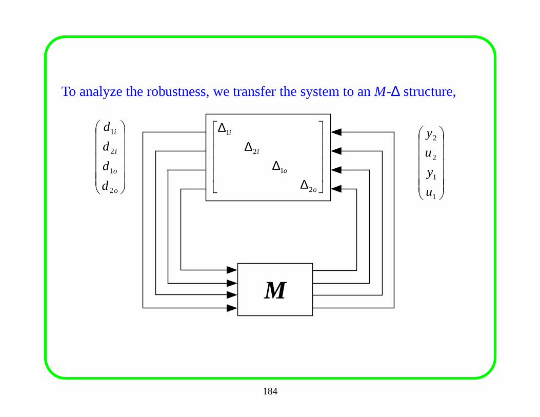
To analyze the robustness, we transfer the system to anM-∆ structure,

M

∆∆

∆∆

o

o

i

i

2

1

2

1

o

o

i

i

d

d

d

d

2

1

2

1

1

1

2

2

u

y

u

y

184

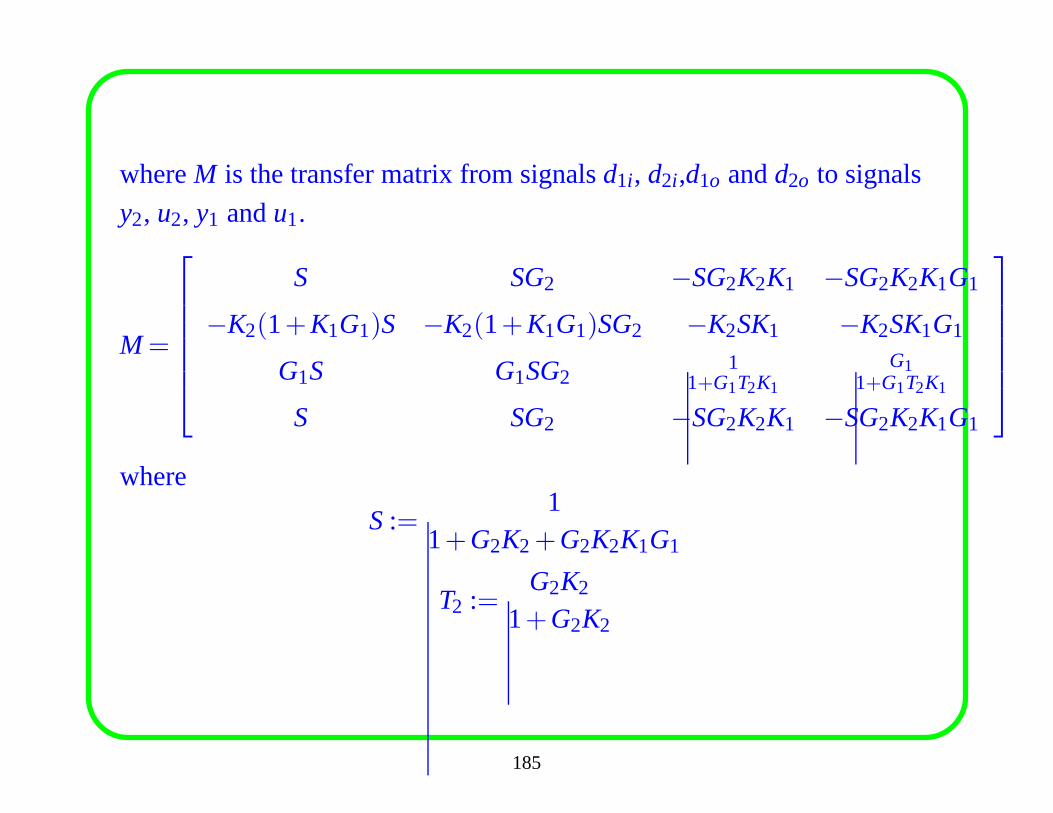
whereM is the transfer matrix from signalsd1i , d2i ,d1o andd2o to signals

y2, u2, y1 andu1.

M =

S SG2 −SG2K2K1 −SG2K2K1G1

−K2(1+K1G1)S −K2(1+K1G1)SG2 −K2SK1 −K2SK1G1

G1S G1SG21

1+G1T2K1

G11+G1T2K1

S SG2 −SG2K2K1 −SG2K2K1G1

where

S:=1

1+G2K2+G2K2K1G1

T2 :=G2K2

1+G2K2

185

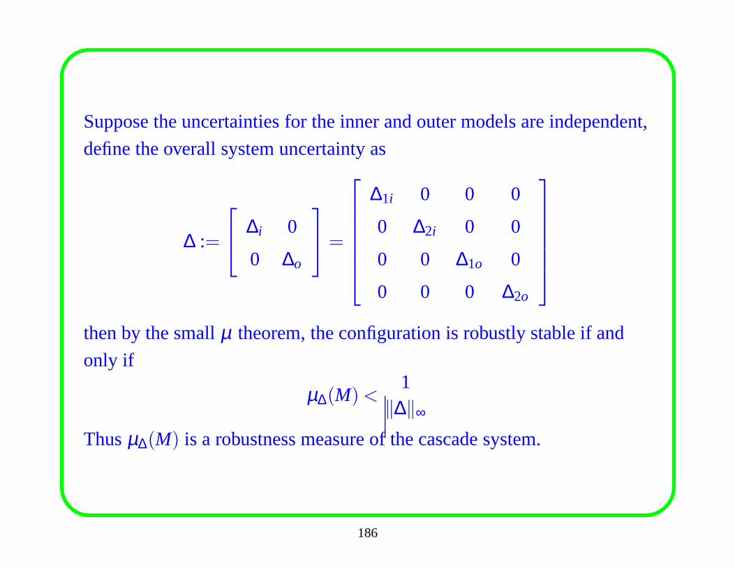
Suppose the uncertainties for the inner and outer models areindependent,

define the overall system uncertainty as

∆ :=

∆i 0

0 ∆o

=

∆1i 0 0 0

0 ∆2i 0 0

0 0 ∆1o 0

0 0 0 ∆2o

then by the smallµ theorem, the configuration is robustly stable if and

only if

µ∆(M)<1

‖∆‖∞

Thusµ∆(M) is a robustness measure of the cascade system.

186

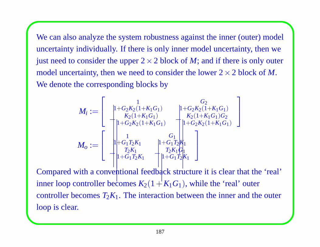
We can also analyze the system robustness against the inner (outer) model

uncertainty individually. If there is only inner model uncertainty, then we

just need to consider the upper 2×2 block ofM; and if there is only outer

model uncertainty, then we need to consider the lower 2×2 block ofM.

We denote the corresponding blocks by

Mi :=

11+G2K2(1+K1G1)

G21+G2K2(1+K1G1)

− K2(1+K1G1)1+G2K2(1+K1G1)

− K2(1+K1G1)G21+G2K2(1+K1G1)

Mo :=

11+G1T2K1

G11+G1T2K1

− T2K11+G1T2K1

− T2K1G11+G1T2K1

Compared with a conventional feedback structure it is clearthat the ‘real’

inner loop controller becomesK2(1+K1G1), while the ‘real’ outer

controller becomesT2K1. The interaction between the inner and the outer

loop is clear.

187

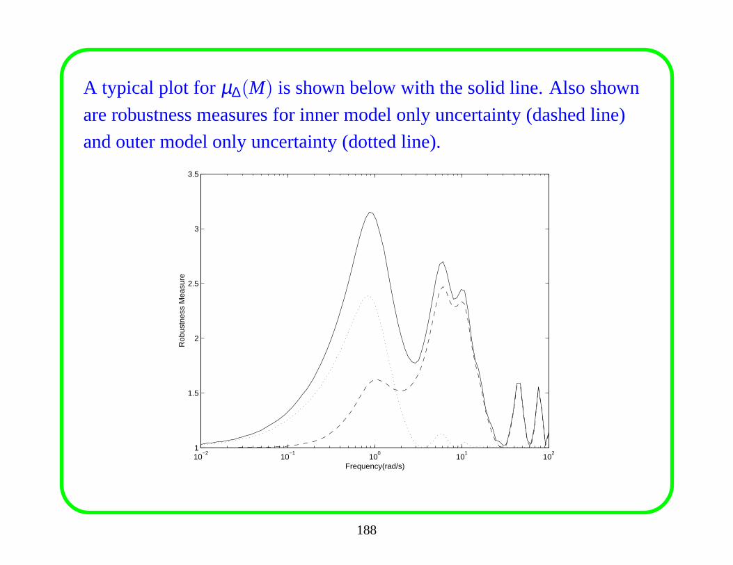
A typical plot for µ∆(M) is shown below with the solid line. Also shown

are robustness measures for inner model only uncertainty (dashed line)

and outer model only uncertainty (dotted line).

10−2

10−1

100

101

102

1

1.5

2

2.5

3

3.5

Frequency(rad/s)

Rob

ustn

ess

Mea

sure

188

It can be observed from this figure:

i) The robustness measure for a cascade structure has two peaks at two

different frequencies, which clearly correspond to the effect of the

inner loop (high frequency peak) and the outer loop (low frequency

peak). This property makes it easy to point out which loop is not

robustly tuned.

ii) The plot also shows the relative interaction between theinner loop

and the outer loop:

• If the inner loop is fast compared with the outer loop, then the

effect of one loop on the other loop is small. In this case the high

peak frequency is away from the low peak frequency.

• If the inner loop is slow, i.e., has almost the same speed as the

outer loop, the effect of one loop on the other loop is large. In this

case the high peak frequency is close to the low peak frequency.

189

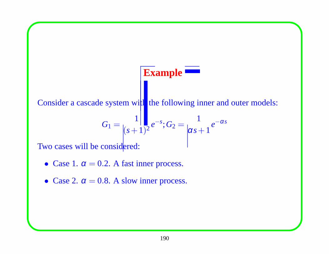
Example

Consider a cascade system with the following inner and outermodels:

G1 =1

(s+1)2 e−s;G2 =1

αs+1e−αs

Two cases will be considered:

• Case 1.α = 0.2. A fast inner process.

• Case 2.α = 0.8. A slow inner process.

190

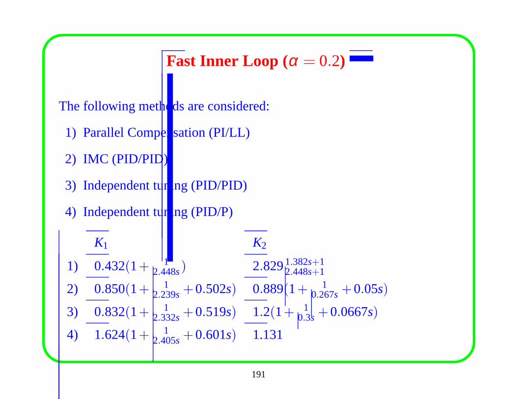
Fast Inner Loop (α = 0.2)

The following methods are considered:

1) Parallel Compensation (PI/LL)

2) IMC (PID/PID)

3) Independent tuning (PID/PID)

4) Independent tuning (PID/P)

K1 K2

1) 0.432(1+ 12.448s) 2.8291.382s+1

2.448s+1

2) 0.850(1+ 12.239s+0.502s) 0.889(1+ 1

0.267s+0.05s)

3) 0.832(1+ 12.332s+0.519s) 1.2(1+ 1

0.3s+0.0667s)

4) 1.624(1+ 12.405s+0.601s) 1.131

191

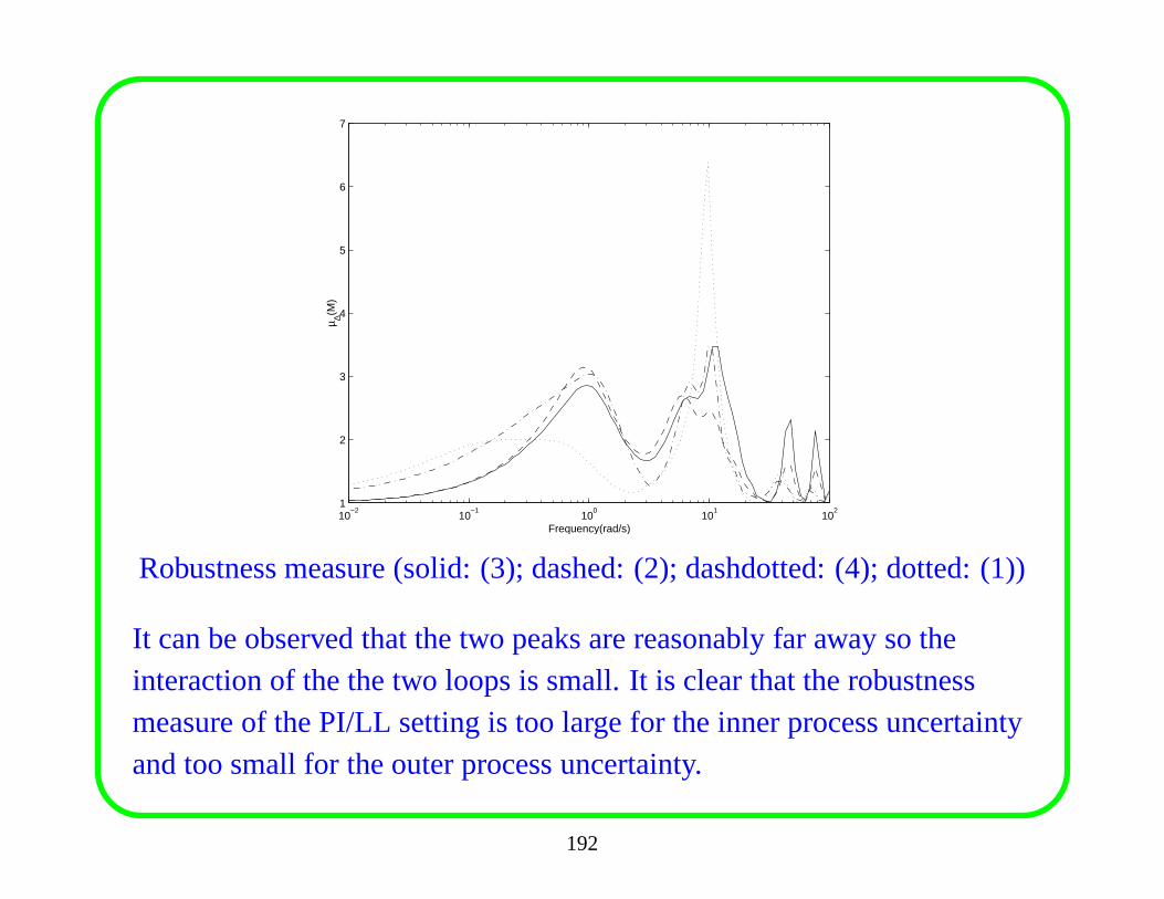
10−2

10−1

100

101

102

1

2

3

4

5

6

7

Frequency(rad/s)

µ ∆(M)

Robustness measure (solid: (3); dashed: (2); dashdotted: (4); dotted: (1))

It can be observed that the two peaks are reasonably far away so theinteraction of the the two loops is small. It is clear that therobustnessmeasure of the PI/LL setting is too large for the inner process uncertaintyand too small for the outer process uncertainty.

192

Performance Analysis

The overall inner loop integral gains of the PI/LL and the independent

tuning (PID/P) settings are 0.499 and 0.764, and those of thePID/PID by

the IMC method and the independent tuning method are 3.547 and 4.363.

It is clear that since PI/LL and PID/P do not have integral action in their

inner loops they have very weak integral actions. Best performance is

achieved by the proposed PID/PID controller due to its largest integral

action.

The step responses for the setpoint and the inner loop disturbance of the

closed-loop systems are shown below. It clearly verifies theclaim above.

193

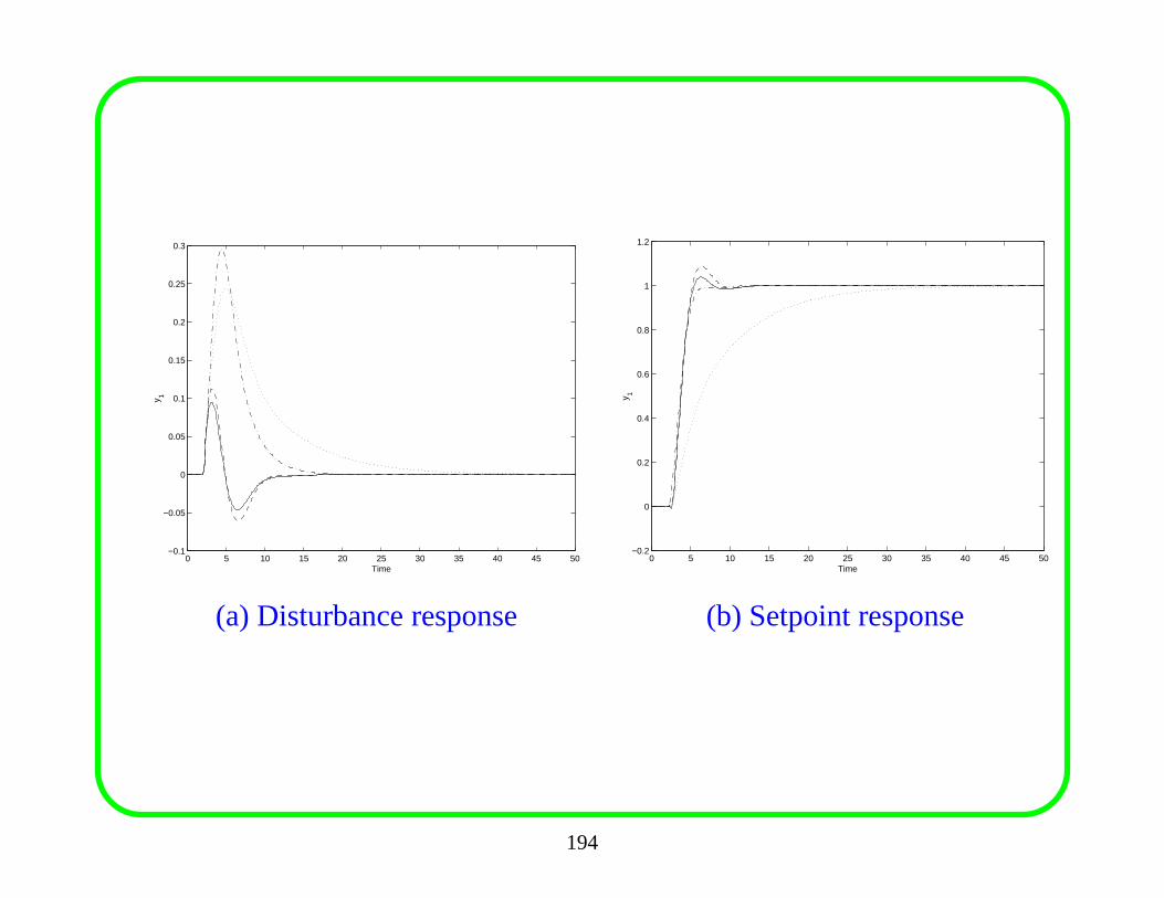
0 5 10 15 20 25 30 35 40 45 50−0.1

−0.05

0

0.05

0.1

0.15

0.2

0.25

0.3

Time

y 1

0 5 10 15 20 25 30 35 40 45 50−0.2

0

0.2

0.4

0.6

0.8

1

1.2

Time

y 1(a) Disturbance response (b) Setpoint response

194

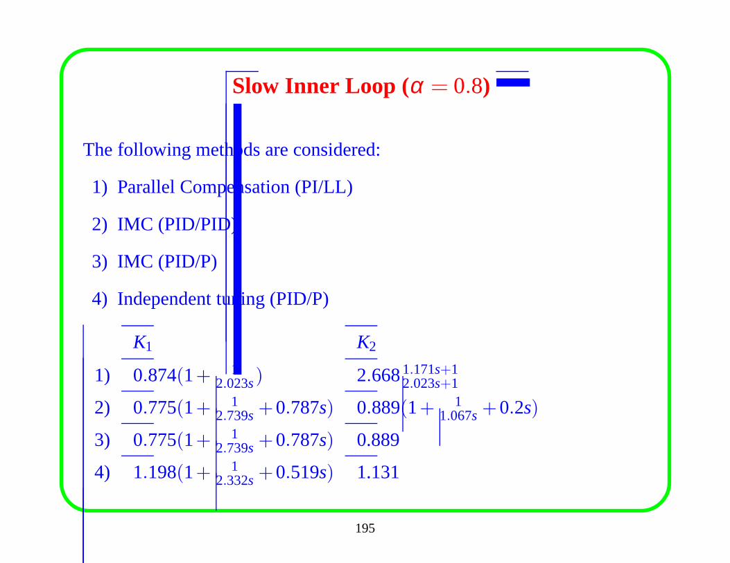
Slow Inner Loop (α = 0.8)

The following methods are considered:

1) Parallel Compensation (PI/LL)

2) IMC (PID/PID)

3) IMC (PID/P)

4) Independent tuning (PID/P)

K1 K2

1) 0.874(1+ 12.023s) 2.6681.171s+1

2.023s+1

2) 0.775(1+ 12.739s+0.787s) 0.889(1+ 1

1.067s+0.2s)

3) 0.775(1+ 12.739s+0.787s) 0.889

4) 1.198(1+ 12.332s+0.519s) 1.131

195

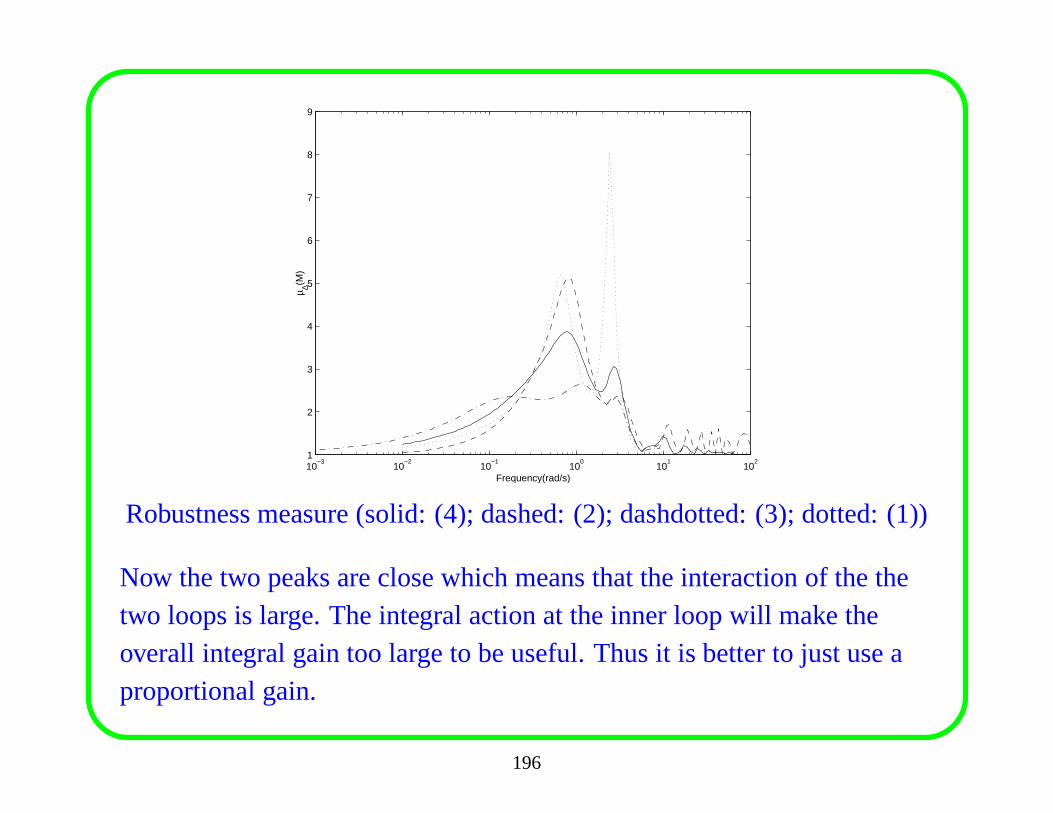
10−3

10−2

10−1

100

101

102

1

2

3

4

5

6

7

8

9

Frequency(rad/s)

µ ∆(M)

Robustness measure (solid: (4); dashed: (2); dashdotted: (3); dotted: (1))

Now the two peaks are close which means that the interaction of the thetwo loops is large. The integral action at the inner loop willmake theoverall integral gain too large to be useful. Thus it is better to just use aproportional gain.

196

Performance Analysis

Now the overall inner loop integral gains of the PI/LL and proposed

PID/P settings are 1.153 and 0.581, and those of the PID/PID and PID/P

by the IMC method are 1.730 and 0.252. The IMC PID/PID controller

has too large integral action at the inner loop so the disturbance response

is oscillatory, while the IMC PID/P has too small integral action so the

response is sluggish.

197

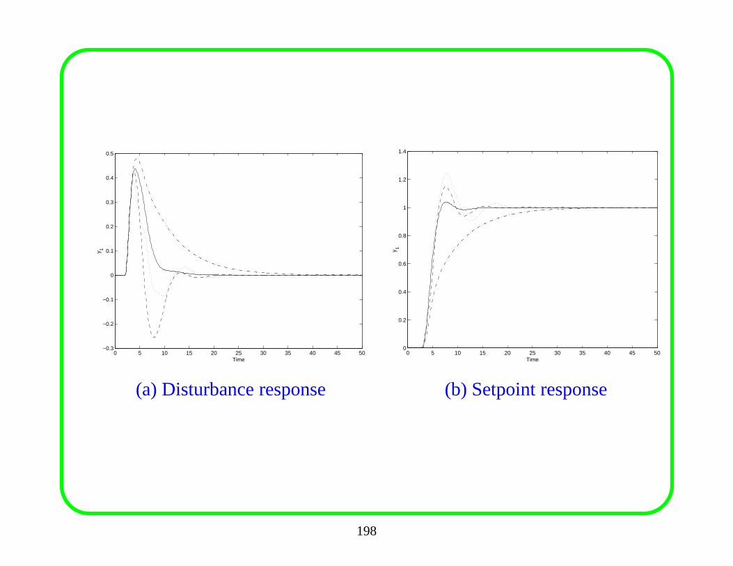
0 5 10 15 20 25 30 35 40 45 50−0.3

−0.2

−0.1

0

0.1

0.2

0.3

0.4

0.5

Time

y 1

0 5 10 15 20 25 30 35 40 45 500

0.2

0.4

0.6

0.8

1

1.2

1.4

Time

y 1(a) Disturbance response (b) Setpoint response

198

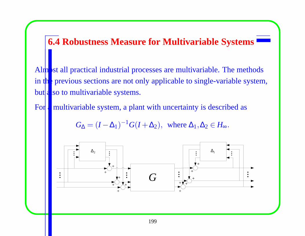
6.4 Robustness Measure for Multivariable Systems

Almost all practical industrial processes are multivariable. The methods

in the previous sections are not only applicable to single-variable system,

but also to multivariable systems.

For a multivariable system, a plant with uncertainty is described as

G∆ = (I −∆1)−1G(I +∆2), where∆1,∆2 ∈ H∞.

G+

+

+

+

+ +

+

+

+++

+

...

......

... ... ...

... ...2∆ 1∆

199

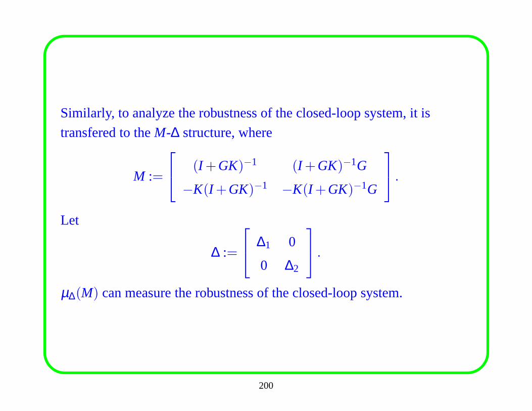
Similarly, to analyze the robustness of the closed-loop system, it is

transfered to theM-∆ structure, where

M :=

(I +GK)−1 (I +GK)−1G

−K(I +GK)−1 −K(I +GK)−1G

.

Let

∆ :=

∆1 0

0 ∆2

.

µ∆(M) can measure the robustness of the closed-loop system.

200

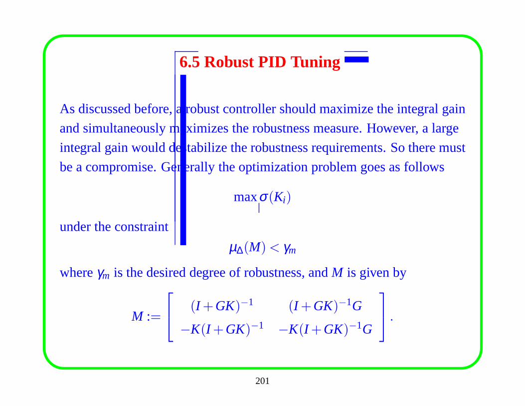
6.5 Robust PID Tuning

As discussed before, a robust controller should maximize the integral gain

and simultaneously maximizes the robustness measure. However, a large

integral gain would destabilize the robustness requirements. So there must

be a compromise. Generally the optimization problem goes asfollows

maxσ(Ki)

under the constraint

µ∆(M)< γm

whereγm is the desired degree of robustness, andM is given by

M :=

(I +GK)−1 (I +GK)−1G

−K(I +GK)−1 −K(I +GK)−1G

.

201

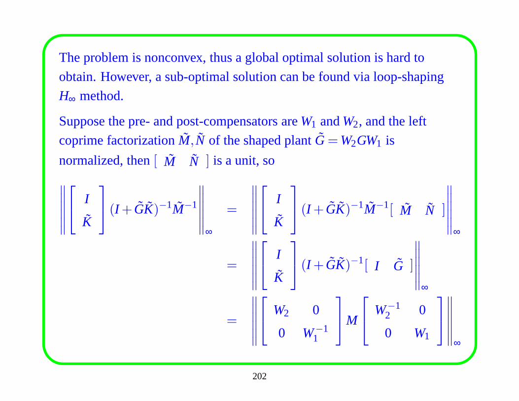
The problem is nonconvex, thus a global optimal solution is hard to

obtain. However, a sub-optimal solution can be found via loop-shaping

H∞ method.

Suppose the pre- and post-compensators areW1 andW2, and the left

coprime factorizationM, N of the shaped plantG=W2GW1 is

normalized, then[ M N ] is a unit, so

∥∥∥∥∥∥

I

K

(I + GK)−1M−1

∥∥∥∥∥∥

∞

=

∥∥∥∥∥∥

I

K

(I + GK)−1M−1[ M N ]

∥∥∥∥∥∥

∞

=

∥∥∥∥∥∥

I

K

(I + GK)−1[ I G ]

∥∥∥∥∥∥

∞

=

∥∥∥∥∥∥

W2 0

0 W−11

M

W−1

2 0

0 W1

∥∥∥∥∥∥

∞

202

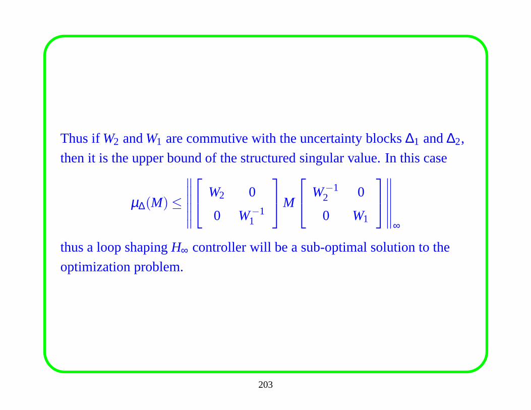
Thus ifW2 andW1 are commutive with the uncertainty blocks∆1 and∆2,

then it is the upper bound of the structured singular value. In this case

µ∆(M)≤

∥∥∥∥∥∥

W2 0

0 W−11

M

W−1

2 0

0 W1

∥∥∥∥∥∥

∞

thus a loop shapingH∞ controller will be a sub-optimal solution to the

optimization problem.

203

PID Tuning via Loop Shaping

In the usual loop-shaping design procedure, the pre-compensator has two

parts

W1 =WaWi

whereWa is usually chosen as a static decoupler andWi is diagonal. For

controller tuning purpose, we can simplify the choice by setting the

post-compensatorW2 as an identity matrix and the pre-compensatorW1 as

a diagonal PI one.

204

The reasons for just using a PI instead of a more sophisticated high-order

pre-compensator are as follows:

1) The final controller will be approximated by a PID one. Comparing

with a simple PI pre-compensator, a high-order pre-compensator

might result in a betterH∞ controller but not a better PID controller

due to the approximation. It may not be worth to find more

sophisticated open-loop shapes.

2) The time-domain performance of the closed-loop system isaffected

by the PI parameters just as in a single-loop process, which makes it

possible to tune the final PID controller by tuning the diagonal PI

pre-compensator.

3) As pointed out in (Skogestad-Postlethwaite:1996) for single-loop

processes, a PI pre-compensator is the ‘best’ for input disturbance

rejection.

205

However,Wa is usually not diagonal, thusW1 does not commute with∆2.

So the uncertainty which theH∞ problem tries to stabilize is only for the

shaped plant, not the actual plant, which is the main source of criticism

for the method. We note that the closed-loop system will showgood

disturbance rejection as long as the integral action is reasonable; the

coupling of the process will only affect the setpoint tracking. So in

loop-shaping design we can first ignore the coupling effect of a

multivariable process, and after the design we can choose a setpoint filter

to modify the setpoint tracking properties.

For example, in a 2×2 system, the final setpoint filter has the following

form:

F =

1 − f1

− f2 1

To completely decouple the setpoint responses,f1 and f2 should be

206

chosen as

f1 = T−111 T12, f2 = T−1

22 T21

whereT is the complementary sensitivity matrix and the subscriptsrefer

to its denoted elements. To realize, a first-order approximation can be

used. Note thatT12 andT21 have derivative action; so the filter will have

the form of asbs+1. In general, we can choose the setpoint filter as

F(s) =

1λ11s+1 − λ12s

λ12s+1

− λ21sλ21s+1

1λ22s+1

where the parameters are tuned to reduce the overshoots and the coupling

in the setpoint responses.

207

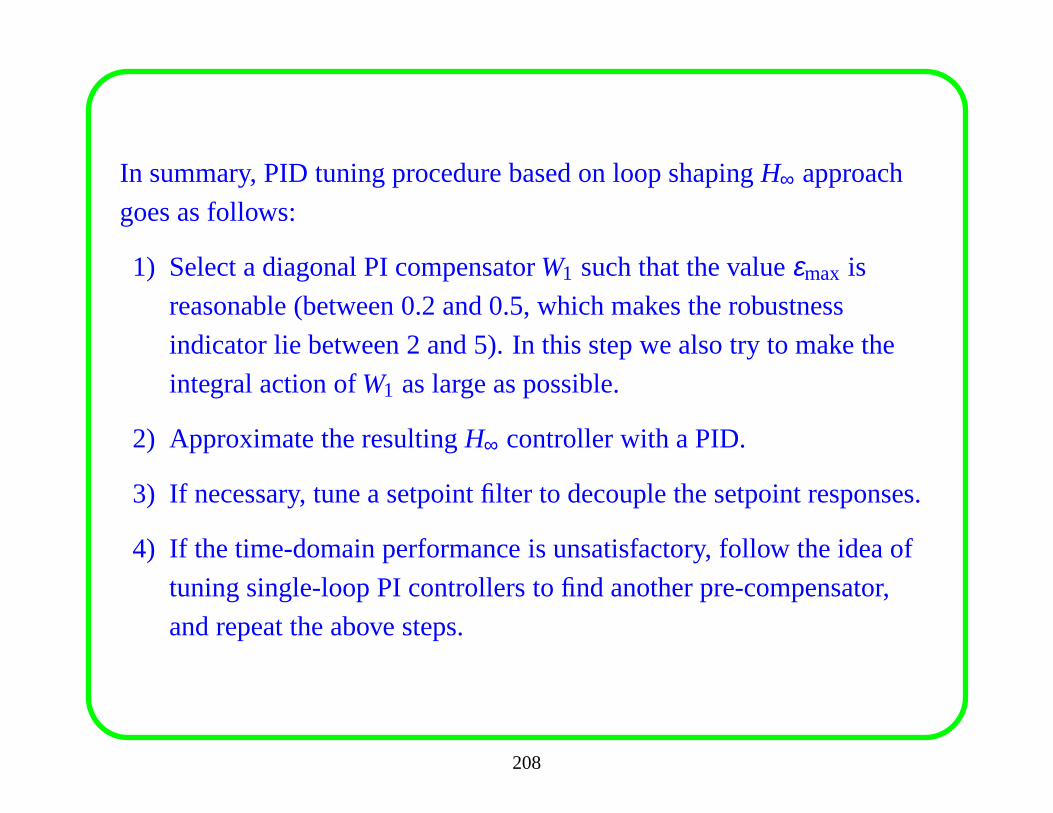
In summary, PID tuning procedure based on loop shapingH∞ approach

goes as follows:

1) Select a diagonal PI compensatorW1 such that the valueεmax is

reasonable (between 0.2 and 0.5, which makes the robustness

indicator lie between 2 and 5). In this step we also try to makethe

integral action ofW1 as large as possible.

2) Approximate the resultingH∞ controller with a PID.

3) If necessary, tune a setpoint filter to decouple the setpoint responses.

4) If the time-domain performance is unsatisfactory, follow the idea of

tuning single-loop PI controllers to find another pre-compensator,

and repeat the above steps.

208

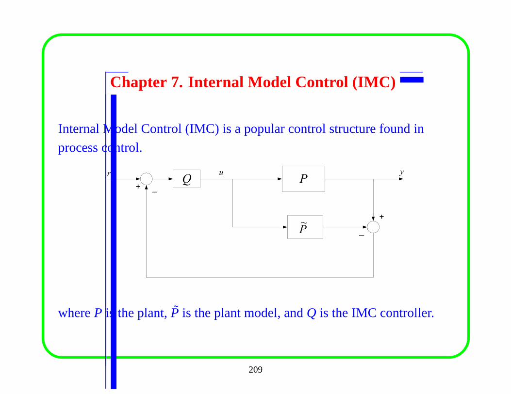
Chapter 7. Internal Model Control (IMC)

Internal Model Control (IMC) is a popular control structurefound in

process control.

Pr y

+

_

_Q

u

+

P~

whereP is the plant,P is the plant model, andQ is the IMC controller.

209

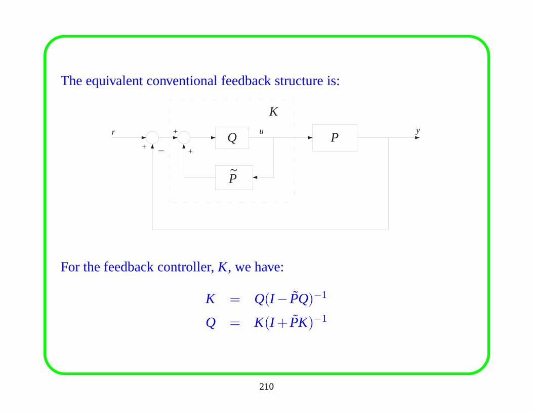
The equivalent conventional feedback structure is:

P r y +

+ _

Q u

+

P ~

K

For the feedback controller,K, we have:

K = Q(I − PQ)−1

Q = K(I + PK)−1

210

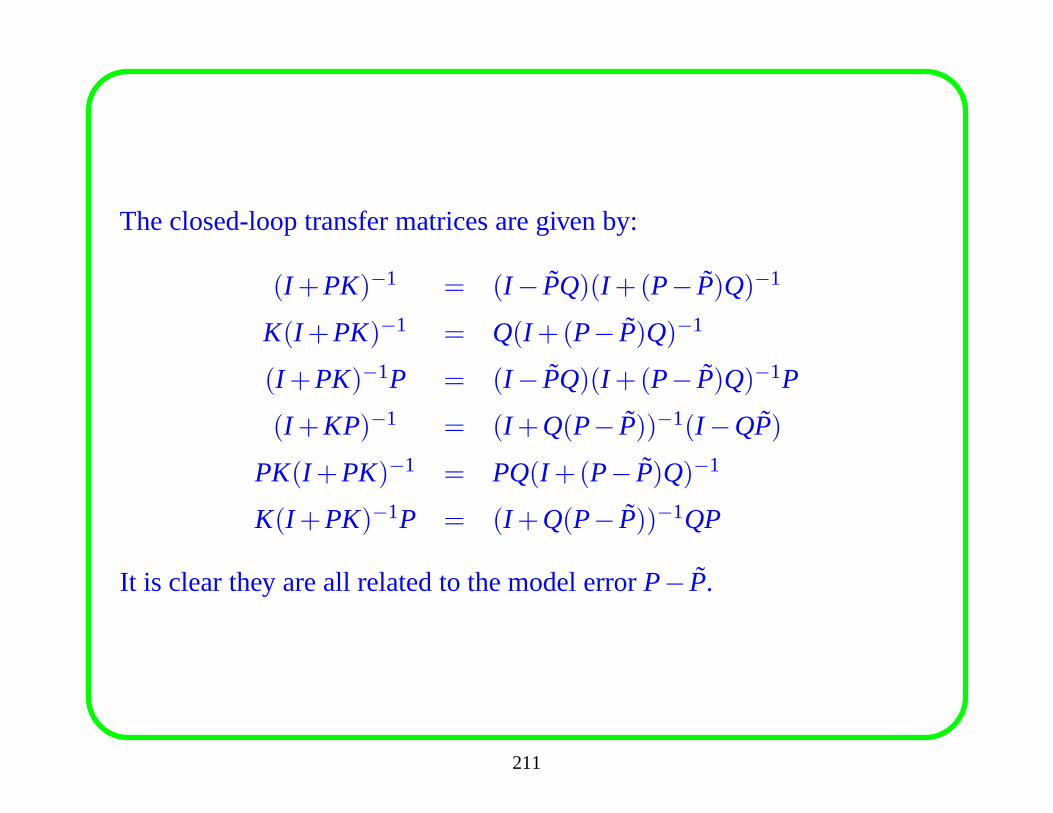
The closed-loop transfer matrices are given by:

(I +PK)−1 = (I − PQ)(I +(P− P)Q)−1

K(I +PK)−1 = Q(I +(P− P)Q)−1

(I +PK)−1P = (I − PQ)(I +(P− P)Q)−1P

(I +KP)−1 = (I +Q(P− P))−1(I −QP)

PK(I +PK)−1 = PQ(I +(P− P)Q)−1

K(I +PK)−1P = (I +Q(P− P))−1QP

It is clear they are all related to the model errorP− P.

211

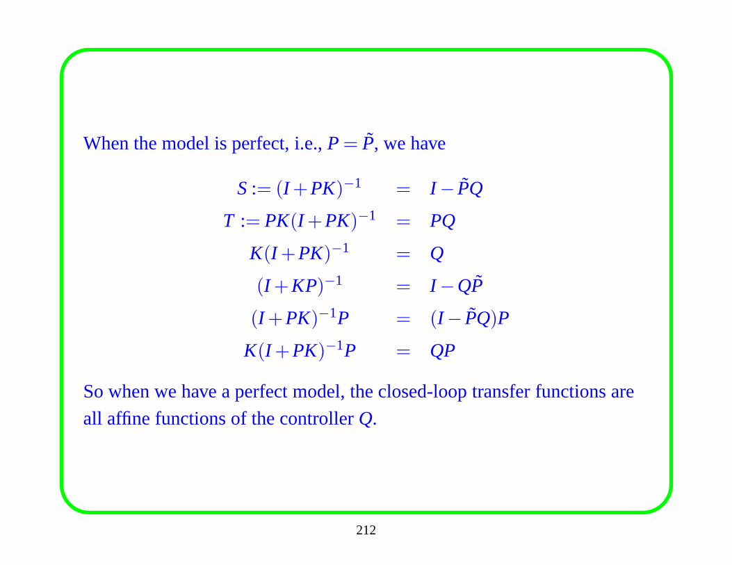
When the model is perfect, i.e.,P= P, we have

S:= (I +PK)−1 = I − PQ

T := PK(I +PK)−1 = PQ

K(I +PK)−1 = Q

(I +KP)−1 = I −QP

(I +PK)−1P = (I − PQ)P

K(I +PK)−1P = QP

So when we have a perfect model, the closed-loop transfer functions are

all affine functions of the controllerQ.

212

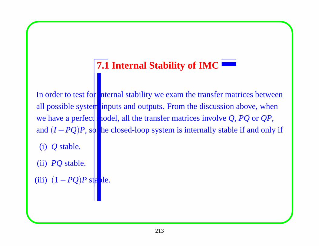
7.1 Internal Stability of IMC

In order to test for internal stability we exam the transfer matrices between

all possible system inputs and outputs. From the discussionabove, when

we have a perfect model, all the transfer matrices involveQ, PQ or QP,

and(I −PQ)P, so the closed-loop system is internally stable if and only if

(i) Q stable.

(ii) PQ stable.

(iii) (1−PQ)P stable.

213

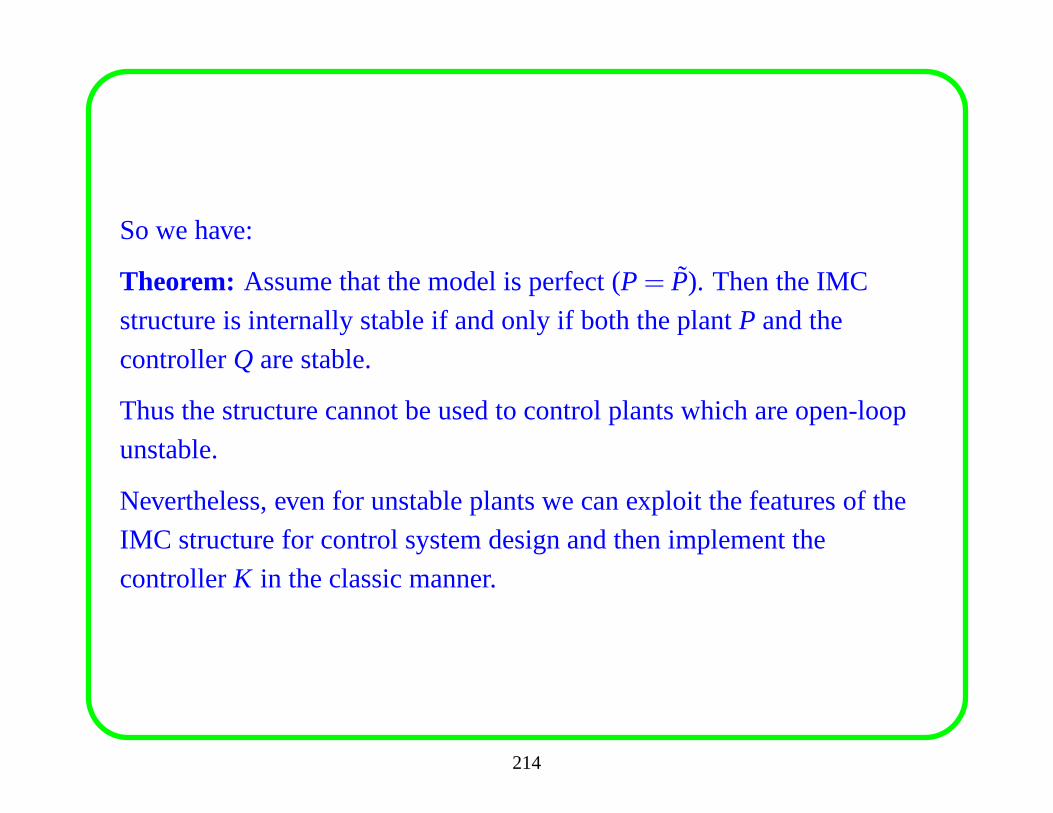
So we have:

Theorem: Assume that the model is perfect (P= P). Then the IMC

structure is internally stable if and only if both the plantP and the

controllerQ are stable.

Thus the structure cannot be used to control plants which areopen-loop

unstable.

Nevertheless, even for unstable plants we can exploit the features of the

IMC structure for control system design and then implement the

controllerK in the classic manner.

214

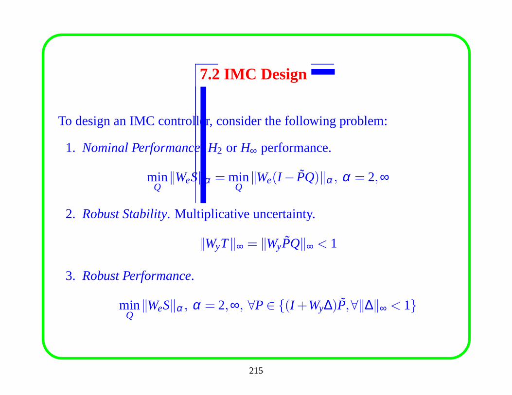
7.2 IMC Design

To design an IMC controller, consider the following problem:

1. Nominal Performance. H2 or H∞ performance.

minQ

‖WeS‖α = minQ

‖We(I − PQ)‖α , α = 2,∞

2. Robust Stability. Multiplicative uncertainty.

‖WyT‖∞ = ‖WyPQ‖∞ < 1

3. Robust Performance.

minQ

‖WeS‖α , α = 2,∞, ∀P∈ {(I +Wy∆)P,∀‖∆‖∞ < 1}

215

Clearly what we need in practice is robust performance. However, for

IMC design, we consider a mixedH2/H∞-type problem for the following

reasons:

• It is hard to solve the optimal robust performance problem (3).

• H2-type performance is an integral-square-error (ISE) objective.

• Since the plant changes and the model quality degrades with time, it

is desirable to provide for convenient on-line robustness adjustment.

To solve the problem, a two-step design method is used. The method has

no inherent optimality characteristics but should providea good

engineering approximation to the optimal solution. It guarantees

robustness but the performance is generally not optimal in any sense.

216

The design procedure goes as follows:

Step 1: Nominal Performance

The controllerQ is selected to yield a “good” system response for the

input(s) of interest, without regard for constraints and model

uncertainty. Generally we will chooseQ such that it is

integral-square-error (ISE) orH2-optimal for a specific set of

reference inputv.

minQ

‖(I − PQ)v‖2

Step 2: Robust Stability and Performance

The aggressive controllerQ obtained in Step 1 is detuned to satisfy

the robustness requirements. For that purposeQ is augmented by a

filter F of fixed structure

Q= QF

217

The filter parameters are adjusted to meet the robustness requirement.

Sometimes a more complicated form is required.

In general, it might not be possible to meet the robust performance

requirement. The reason could be that the design procedure fails to

produce an acceptableQ.

On the other hand, there might not exist anyQ such that the

requirement is satisfied. Then the performance requirements have to

be relaxed and/or the model uncertainty has to be reduced.

218

Nominal Performance

Nominal performance can be guaranteed by solving theH2-optimization

problem. Generally the plantP can be factored into a stable all-pass

portionPA and an minimum-phase (MP) portionPM such that

P= PAPM

HerePA andPM are stable andPHA ( jω)PA( jω) = I .

Similarly, the set of inputsv can be factored as

v= vMvA

wherevM is minimum-phase andvA is all-pass.

219

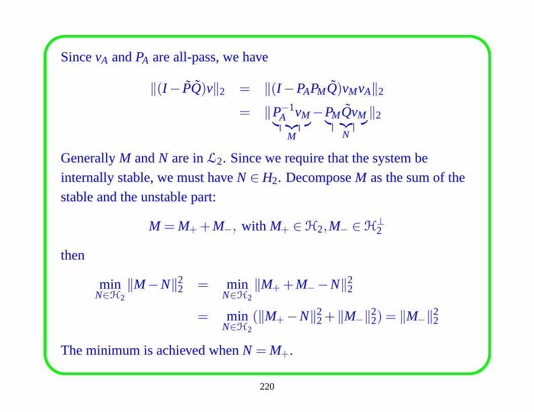
SincevA andPA are all-pass, we have

‖(I − PQ)v‖2 = ‖(I −PAPMQ)vMvA‖2

= ‖P−1A vM︸ ︷︷ ︸

M

−PMQvM︸ ︷︷ ︸

N

‖2

GenerallyM andN are inL2. Since we require that the system beinternally stable, we must haveN ∈ H2. DecomposeM as the sum of thestable and the unstable part:

M = M++M−, with M+ ∈H2,M− ∈H⊥2

then

minN∈H2

‖M−N‖22 = min

N∈H2‖M++M−−N‖2

2

= minN∈H2

(‖M+−N‖22+‖M−‖2

2) = ‖M−‖22

The minimum is achieved whenN = M+.

220

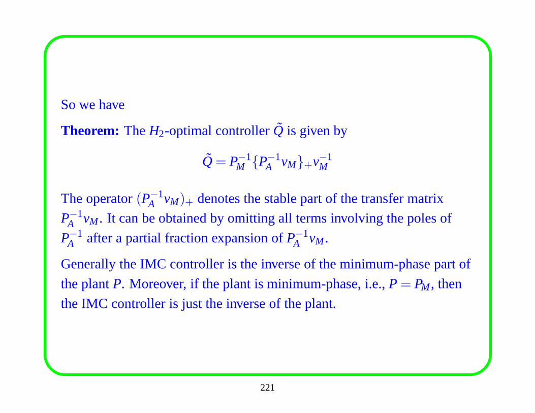
So we have

Theorem: TheH2-optimal controllerQ is given by

Q= P−1M {P−1

A vM}+v−1M

The operator(P−1A vM)+ denotes the stable part of the transfer matrix

P−1A vM. It can be obtained by omitting all terms involving the polesof

P−1A after a partial fraction expansion ofP−1

A vM.

Generally the IMC controller is the inverse of the minimum-phase part of

the plantP. Moreover, if the plant is minimum-phase, i.e.,P= PM, then

the IMC controller is just the inverse of the plant.

221

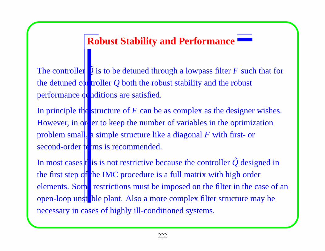
Robust Stability and Performance

The controllerQ is to be detuned through a lowpass filterF such that for

the detuned controllerQ both the robust stability and the robust

performance conditions are satisfied.

In principle the structure ofF can be as complex as the designer wishes.

However, in order to keep the number of variables in the optimization

problem small, a simple structure like a diagonalF with first- or

second-order terms is recommended.

In most cases this is not restrictive because the controllerQ designed in

the first step of the IMC procedure is a full matrix with high order

elements. Some restrictions must be imposed on the filter in the case of an

open-loop unstable plant. Also a more complex filter structure may be

necessary in cases of highly ill-conditioned systems.

222

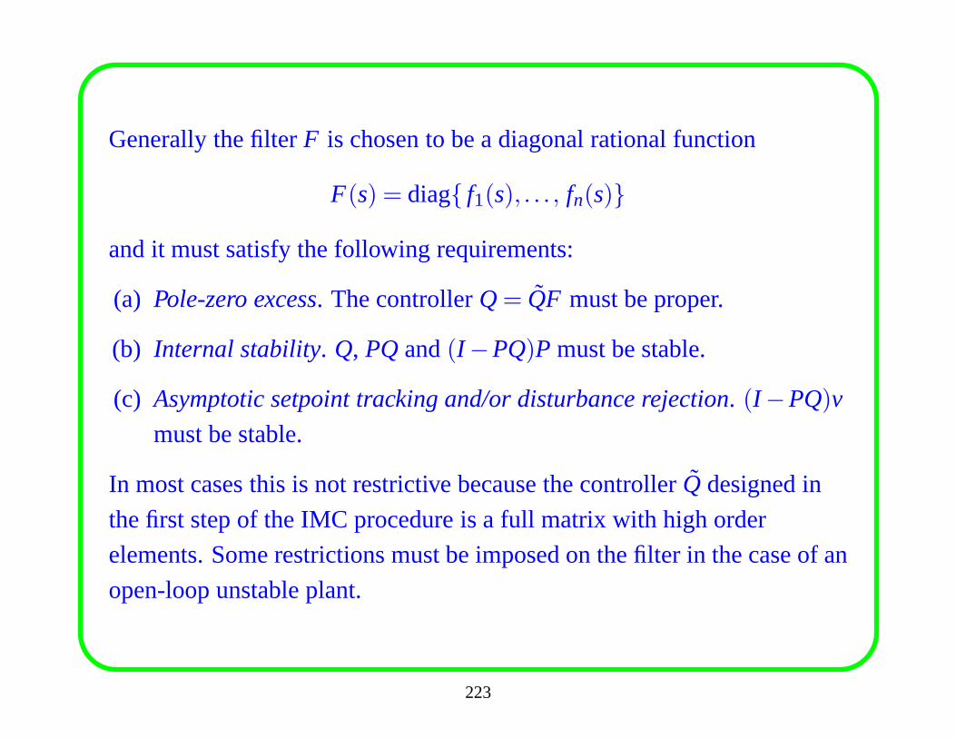
Generally the filterF is chosen to be a diagonal rational function

F(s) = diag{ f1(s), . . . , fn(s)}

and it must satisfy the following requirements:

(a) Pole-zero excess. The controllerQ= QF must be proper.

(b) Internal stability. Q, PQand(I −PQ)P must be stable.

(c) Asymptotic setpoint tracking and/or disturbance rejection. (I −PQ)v

must be stable.

In most cases this is not restrictive because the controllerQ designed in

the first step of the IMC procedure is a full matrix with high order

elements. Some restrictions must be imposed on the filter in the case of an

open-loop unstable plant.

223

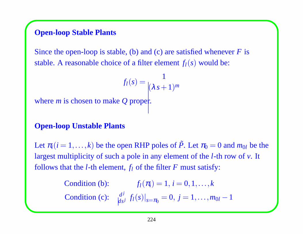
Open-loop Stable Plants

Since the open-loop is stable, (b) and (c) are satisfied whenever F isstable. A reasonable choice of a filter elementfl (s) would be:

fl (s) =1

(λs+1)m

wherem is chosen to makeQ proper.

Open-loop Unstable Plants

Let πi(i = 1, . . . ,k) be the open RHP poles ofP. Let π0 = 0 andm0l be thelargest multiplicity of such a pole in any element of thel -th row ofv. Itfollows that thel -th element,fl of the filterF must satisfy:

Condition (b): fl (πi) = 1, i = 0,1, . . . ,k

Condition (c): d j

dsj fl (s)|s=π0= 0, j = 1, . . . ,m0l −1

224

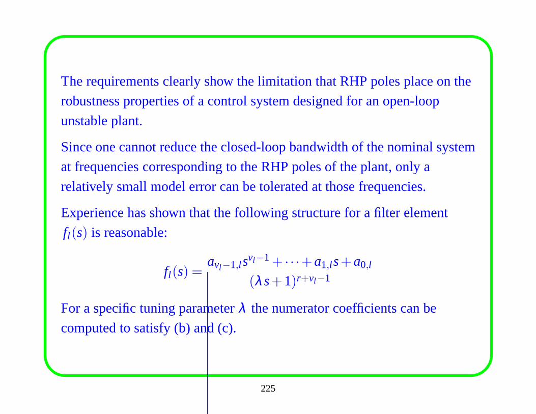
The requirements clearly show the limitation that RHP polesplace on the

robustness properties of a control system designed for an open-loop

unstable plant.

Since one cannot reduce the closed-loop bandwidth of the nominal system

at frequencies corresponding to the RHP poles of the plant, only a

relatively small model error can be tolerated at those frequencies.

Experience has shown that the following structure for a filter element

fl (s) is reasonable:

fl (s) =avl−1,l svl−1+ · · ·+a1,l s+a0,l

(λs+1)r+vl−1

For a specific tuning parameterλ the numerator coefficients can be

computed to satisfy (b) and (c).

225

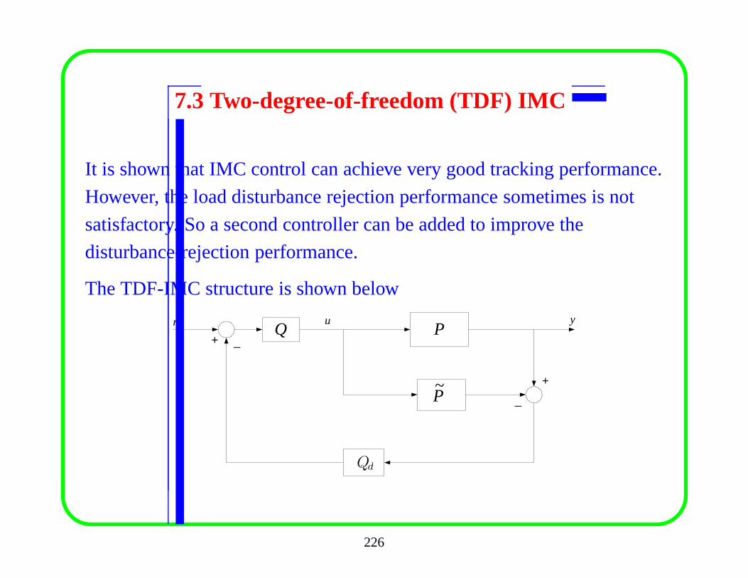
7.3 Two-degree-of-freedom (TDF) IMC

It is shown that IMC control can achieve very good tracking performance.

However, the load disturbance rejection performance sometimes is not

satisfactory. So a second controller can be added to improvethe

disturbance-rejection performance.

The TDF-IMC structure is shown below

Pr y

+

_

_Q

u

+

P~

Qd

226

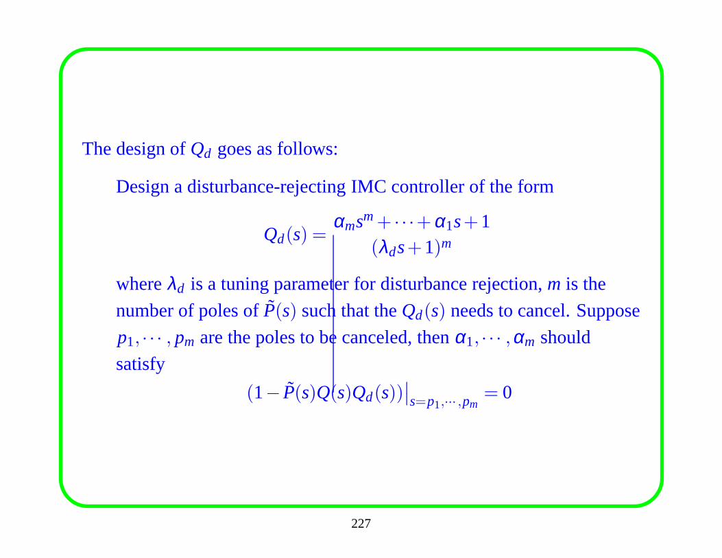
The design ofQd goes as follows:

Design a disturbance-rejecting IMC controller of the form

Qd(s) =αmsm+ · · ·+α1s+1

(λds+1)m

whereλd is a tuning parameter for disturbance rejection,m is the

number of poles ofP(s) such that theQd(s) needs to cancel. Suppose

p1, · · · , pm are the poles to be canceled, thenα1, · · · ,αm should

satisfy

(1− P(s)Q(s)Qd(s))∣∣s=p1,··· ,pm

= 0

227

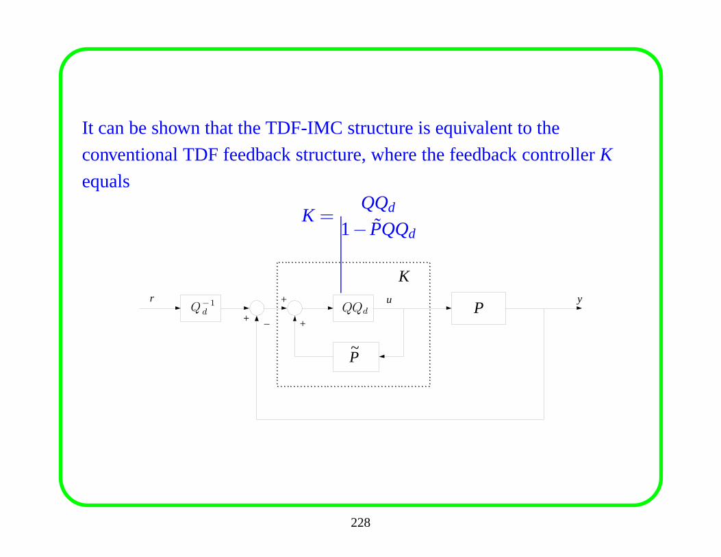
It can be shown that the TDF-IMC structure is equivalent to the

conventional TDF feedback structure, where the feedback controller K

equals

K =QQd

1− PQQd

Pr y+

+_

u

+

P~

K

Q¡1

d QQd

228

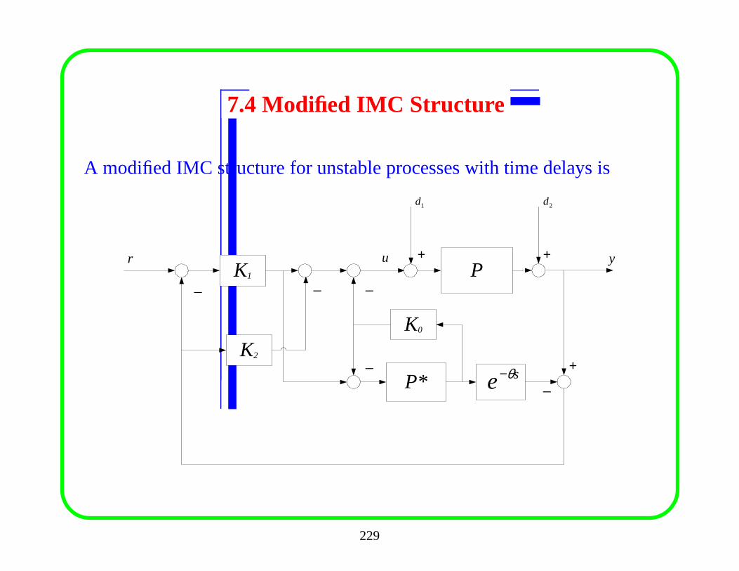
7.4 Modified IMC Structure

A modified IMC structure for unstable processes with time delays is

P

P*

r y

+_

_

1d 2d

++

K2

_K1

K0

_

_se θ−

u

229

The advantages of the modified IMC structure are:

• IMC structure can be retained for unstable processes. Controllers do

not have to be converted to conventional ones for implementation.

• Setpoint tracking and disturbance rejection can be designed

separately. The setpoint tracking design follows the standard IMC

design for a stable plant.

• Robustness and disturbance rejection mainly rely on a controller in a

feedback loop. Robustness of the whole structure can be considered

by tuning this controller.

230

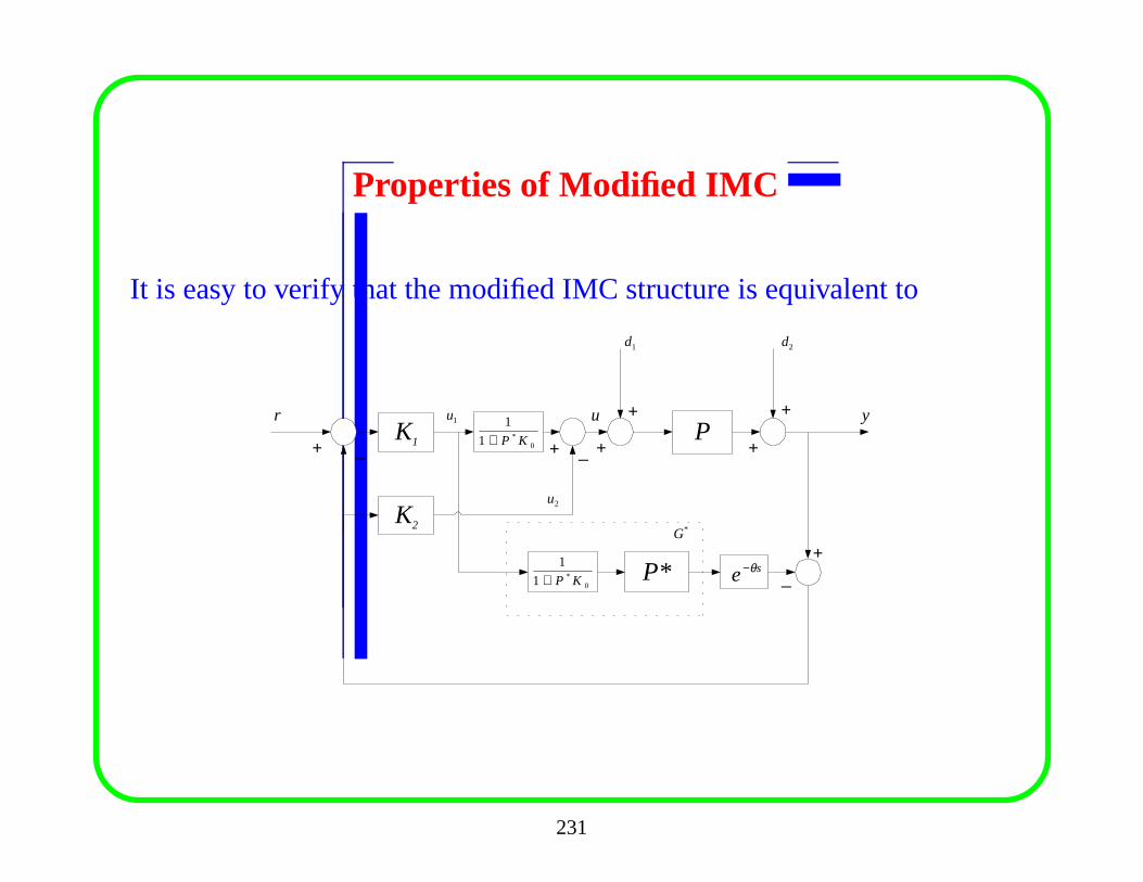
Properties of Modified IMC

It is easy to verify that the modified IMC structure is equivalent to

P

P* se θ−

r y

+

_

_

1d 2d

++

K2

_K1

u

0*1

1

KP+

*G

1u

2u

0*1

1

KP+

+ + ++

231

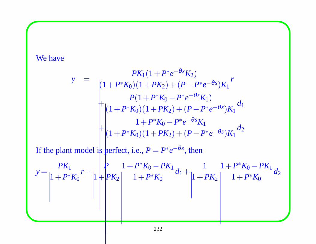
We have

y =PK1(1+P∗e−θsK2)

(1+P∗K0)(1+PK2)+(P−P∗e−θs)K1r

+P(1+P∗K0−P∗e−θsK1)

(1+P∗K0)(1+PK2)+(P−P∗e−θs)K1d1

+1+P∗K0−P∗e−θsK1

(1+P∗K0)(1+PK2)+(P−P∗e−θs)K1d2

If the plant model is perfect, i.e.,P= P∗e−θs, then

y=PK1

1+P∗K0r+

P1+PK2

1+P∗K0−PK1

1+P∗K0d1+

11+PK2

1+P∗K0−PK1

1+P∗K0d2

232

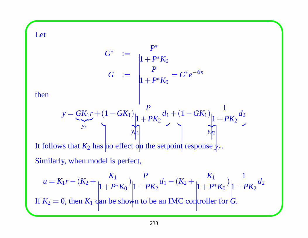
Let

G∗ :=P∗

1+P∗K0

G :=P

1+P∗K0= G∗e−θs

then

y= GK1r︸ ︷︷ ︸

yr

+(1−GK1)P

1+PK2d1

︸ ︷︷ ︸

yd1

+(1−GK1)1

1+PK2d2

︸ ︷︷ ︸

yd2

It follows thatK2 has no effect on the setpoint responseyr .

Similarly, when model is perfect,

u= K1r − (K2+K1

1+P∗K0)

P1+PK2

d1− (K2+K1

1+P∗K0)

11+PK2

d2

If K2 = 0, thenK1 can be shown to be an IMC controller forG.

233

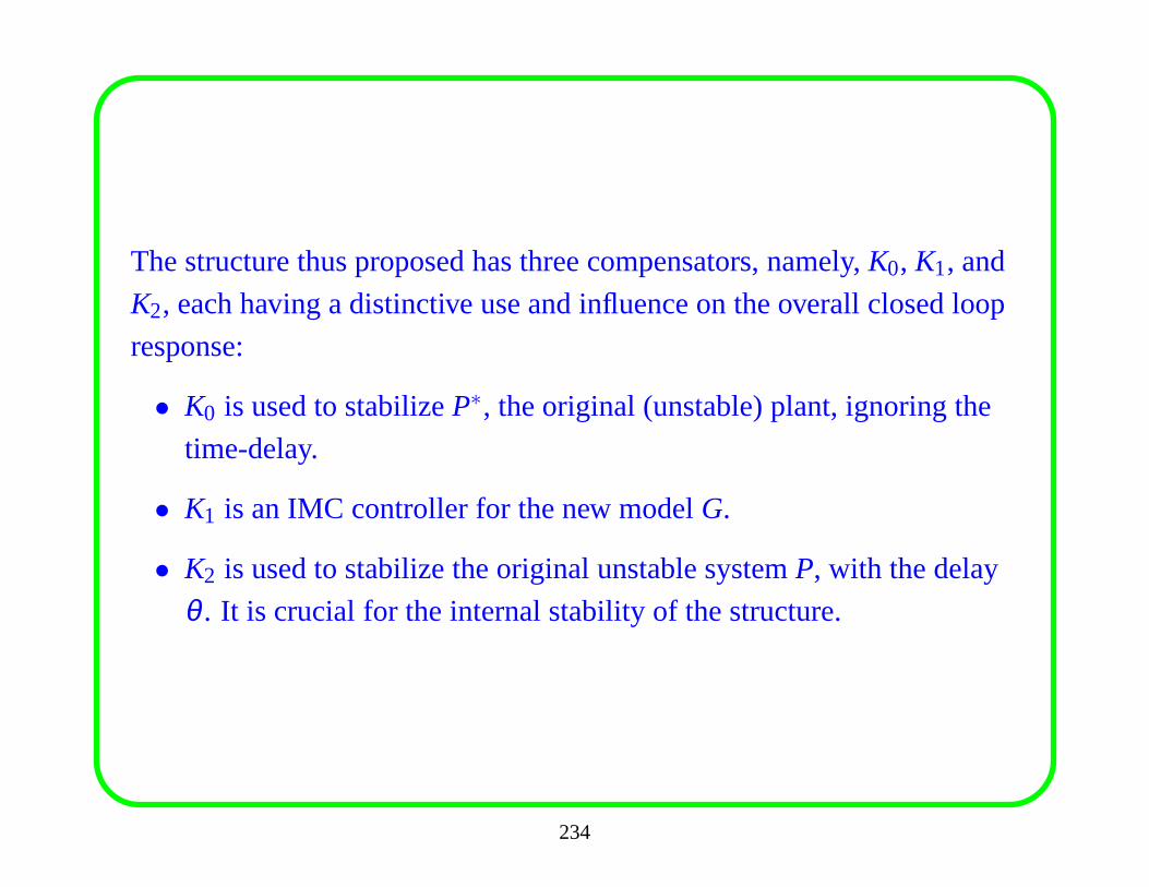
The structure thus proposed has three compensators, namely, K0, K1, and

K2, each having a distinctive use and influence on the overall closed loop

response:

• K0 is used to stabilizeP∗, the original (unstable) plant, ignoring the

time-delay.

• K1 is an IMC controller for the new modelG.

• K2 is used to stabilize the original unstable systemP, with the delay

θ . It is crucial for the internal stability of the structure.

234

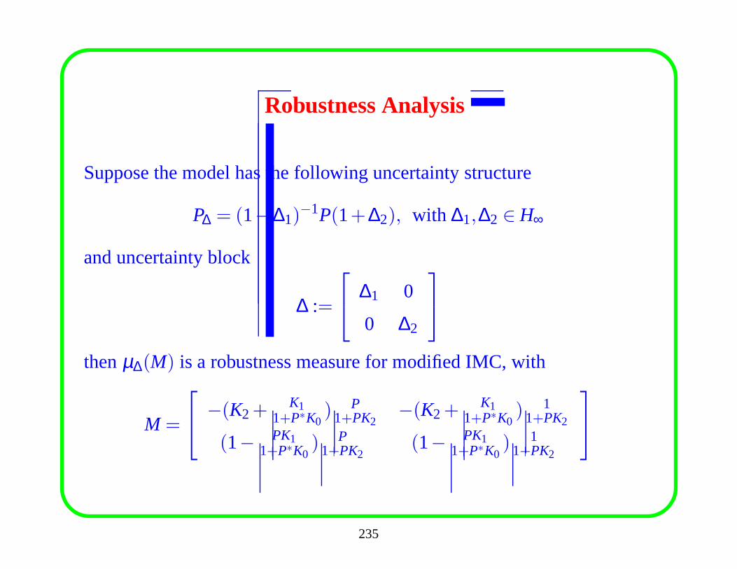
Robustness Analysis

Suppose the model has the following uncertainty structure

P∆ = (1−∆1)−1P(1+∆2), with ∆1,∆2 ∈ H∞

and uncertainty block

∆ :=

∆1 0

0 ∆2

thenµ∆(M) is a robustness measure for modified IMC, with

M =

−(K2+

K11+P∗K0

) P1+PK2

−(K2+K1

1+P∗K0) 1

1+PK2

(1− PK11+P∗K0

) P1+PK2

(1− PK11+P∗K0

) 11+PK2

235

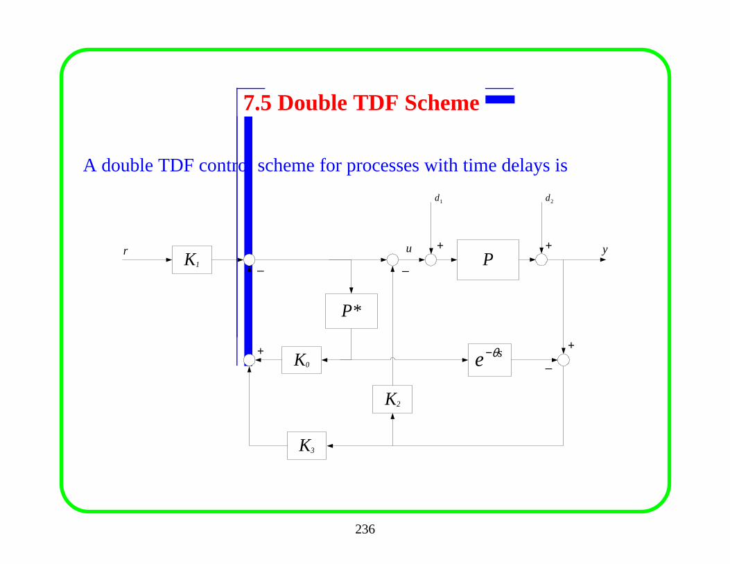
7.5 Double TDF Scheme

A double TDF control scheme for processes with time delays is

P

P*

r y

+_

_

1d 2d

++

K2

K1

K0

_

+ se θ−

u

K3

236

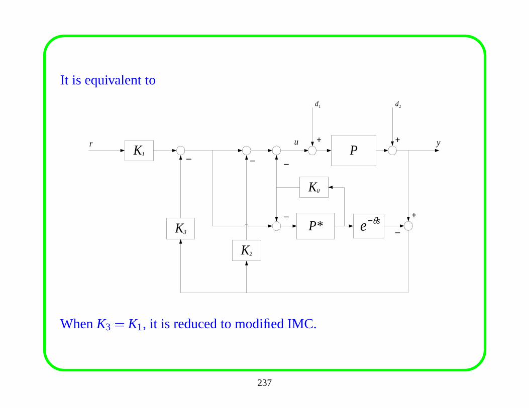
It is equivalent to

P

P*

r y

+_

_

1d 2d

++

K2

_K1

K0

_

_se θ−

u

K3

WhenK3 = K1, it is reduced to modified IMC.

237

Chapter 8. Wide-Range Robust Control

Robust controller synthesis aims to achieve acceptable performance under

model uncertainties. A common source of model uncertainties is the

change of operating points due to system nonlinearity. If a process has

severe nonlinearity, then a single robust controller may not achieve global

performance, hence wide-range robust controllers are required.

• Gain scheduling control is a possible method to achieve wide-range

performance, however gain scheduling needs to have a detailed

nonlinear model or complete knowledge of the operating points,

which is not practical. Moreover, the cost of implementing again

scheduling controller is high.

238

• Another possible method to achieve wide-range performanceis to

use multi-model control. The method divides the operating range into

several ‘linear’ range, and designs linear controllers at each local

operating point, and combines them into a multi-model controller.

The idea is simple and the simulation results shown that the method

is effective.

• A still simpler method is to ‘avoid’ the nonlinearity of a unit by

carefully choosing the operating points. The idea is that some of the

operating points are seldom met in practice so even if the linear

controller may not work well under such operating points it can still

get good global performance as long as the controller does not enter

such an operating range.

239

8.1 Gap Metric

The robust control design techniques assume that we have some

description of the model uncertainties (i.e., we have a measure of the

distance from the nominal plant to the set of uncertainty systems). This

measure is usually chosen to be a metric or a norm (e.g.,H∞-norm).

However, theH∞ norm can be a poor measure of the distance between

systems with respect to feedback control system design.

240

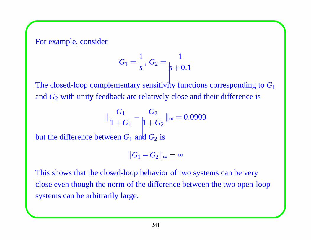
For example, consider

G1 =1s, G2 =

1s+0.1

The closed-loop complementary sensitivity functions corresponding toG1

andG2 with unity feedback are relatively close and their difference is

‖ G1

1+G1− G2

1+G2‖∞ = 0.0909

but the difference betweenG1 andG2 is

‖G1−G2‖∞ = ∞

This shows that the closed-loop behavior of two systems can be very

close even though the norm of the difference between the two open-loop

systems can be arbitrarily large.

241

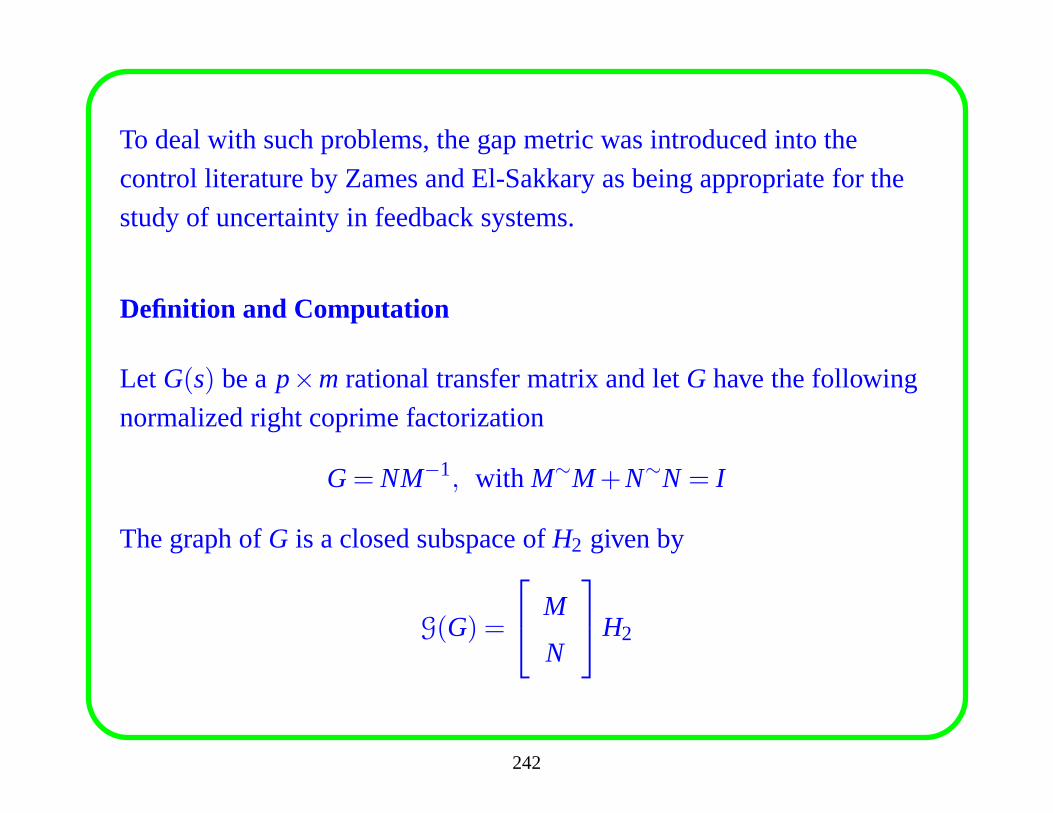
To deal with such problems, the gap metric was introduced into the

control literature by Zames and El-Sakkary as being appropriate for the

study of uncertainty in feedback systems.

Definition and Computation

Let G(s) be ap×m rational transfer matrix and letG have the following

normalized right coprime factorization

G= NM−1, with M∼M+N∼N = I

The graph ofG is a closed subspace ofH2 given by

G(G) =

M

N

H2

242

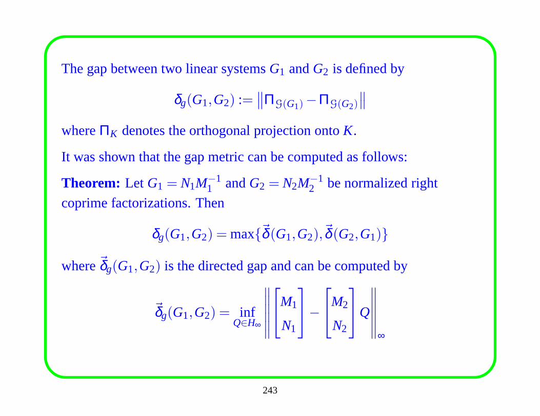
The gap between two linear systemsG1 andG2 is defined by

δg(G1,G2) :=∥∥ΠG(G1)−ΠG(G2)

∥∥

whereΠK denotes the orthogonal projection ontoK.

It was shown that the gap metric can be computed as follows:

Theorem: Let G1 = N1M−11 andG2 = N2M−1

2 be normalized right

coprime factorizations. Then

δg(G1,G2) = max{~δ (G1,G2),~δ (G2,G1)}

where~δg(G1,G2) is the directed gap and can be computed by

~δg(G1,G2) = infQ∈H∞

∥∥∥∥∥∥

M1

N1

−

M2

N2

Q

∥∥∥∥∥∥

∞

243

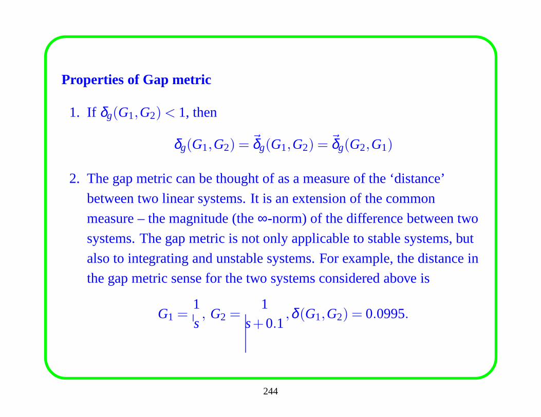
Properties of Gap metric

1. If δg(G1,G2)< 1, then

δg(G1,G2) = ~δg(G1,G2) = ~δg(G2,G1)

2. The gap metric can be thought of as a measure of the ‘distance’

between two linear systems. It is an extension of the common

measure – the magnitude (the∞-norm) of the difference between two

systems. The gap metric is not only applicable to stable systems, but

also to integrating and unstable systems. For example, the distance in

the gap metric sense for the two systems considered above is

G1 =1s, G2 =

1s+0.1

,δ (G1,G2) = 0.0995.

244

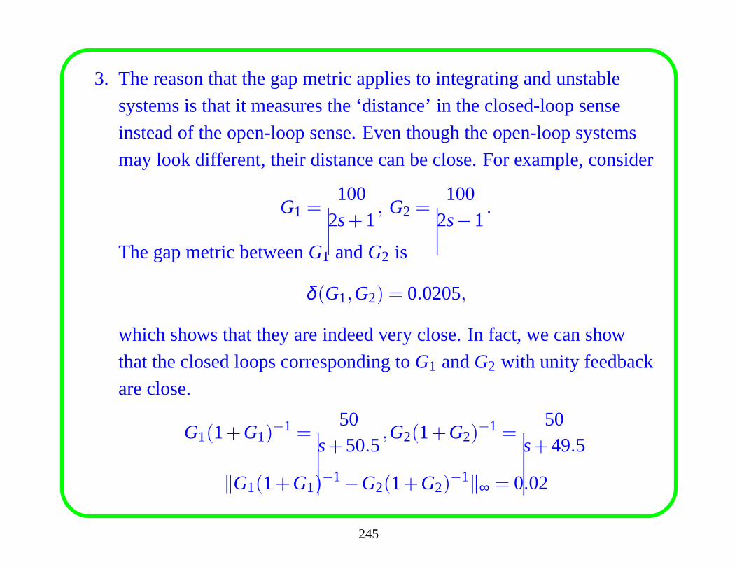
3. The reason that the gap metric applies to integrating and unstable

systems is that it measures the ‘distance’ in the closed-loop sense

instead of the open-loop sense. Even though the open-loop systems

may look different, their distance can be close. For example, consider

G1 =100

2s+1, G2 =

1002s−1

.

The gap metric betweenG1 andG2 is

δ (G1,G2) = 0.0205,

which shows that they are indeed very close. In fact, we can show

that the closed loops corresponding toG1 andG2 with unity feedback

are close.

G1(1+G1)−1 =

50s+50.5

,G2(1+G2)−1 =

50s+49.5

‖G1(1+G1)−1−G2(1+G2)

−1‖∞ = 0.02

245

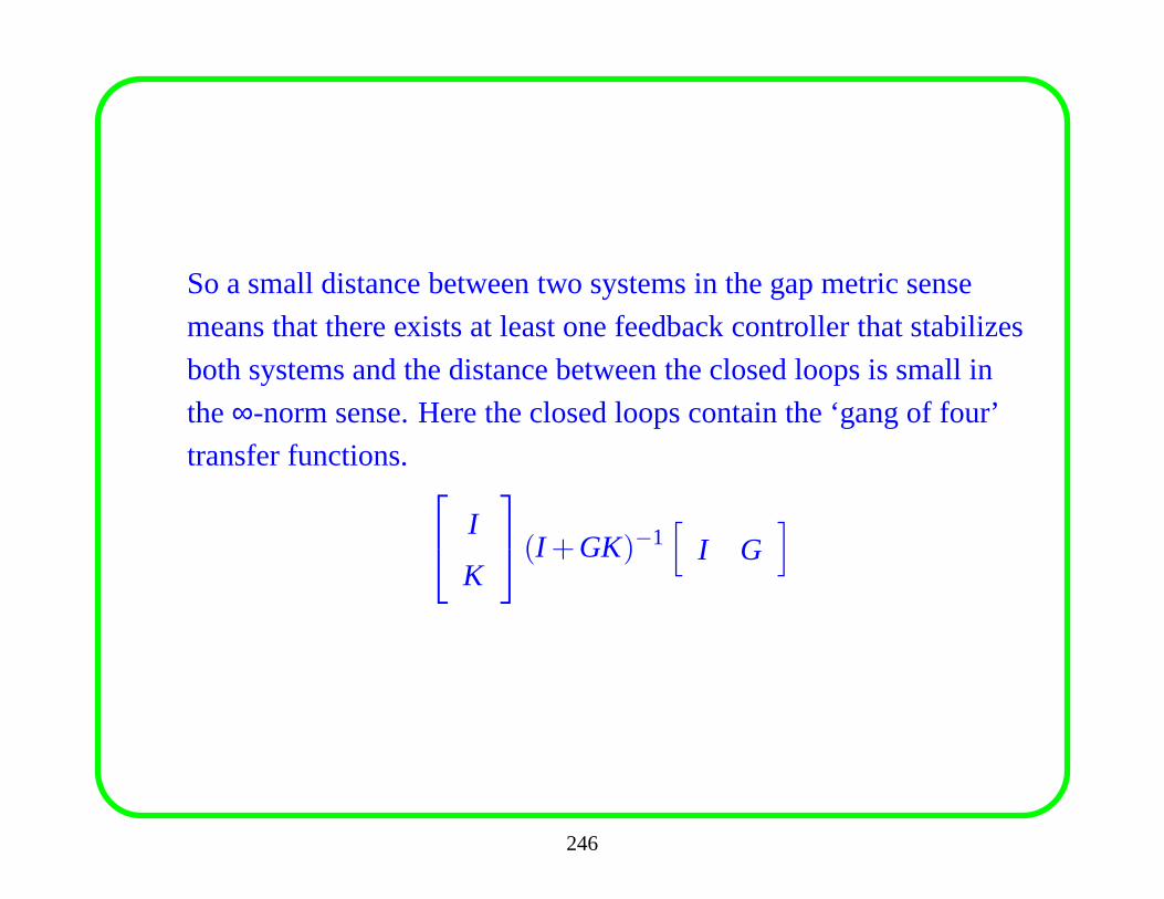
So a small distance between two systems in the gap metric sense

means that there exists at least one feedback controller that stabilizes

both systems and the distance between the closed loops is small in

the∞-norm sense. Here the closed loops contain the ‘gang of four’

transfer functions.

I

K

(I +GK)−1[

I G]

246

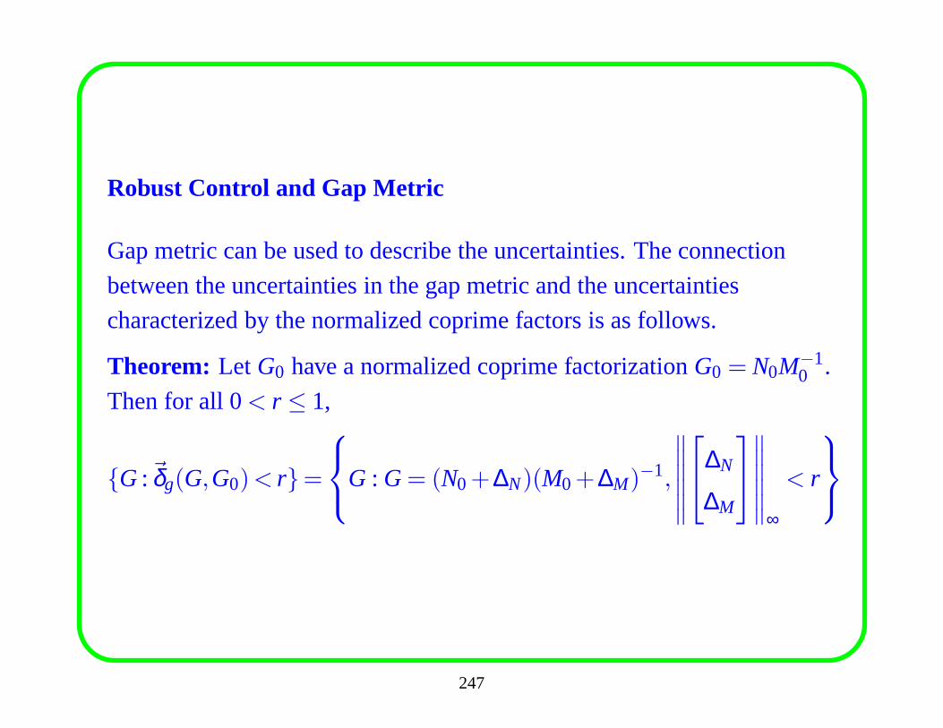
Robust Control and Gap Metric

Gap metric can be used to describe the uncertainties. The connection

between the uncertainties in the gap metric and the uncertainties

characterized by the normalized coprime factors is as follows.

Theorem: Let G0 have a normalized coprime factorizationG0 = N0M−10 .

Then for all 0< r ≤ 1,

{G :~δg(G,G0)< r}=

G : G= (N0+∆N)(M0+∆M)−1,

∥∥∥∥∥∥

∆N

∆M

∥∥∥∥∥∥

∞

< r

247

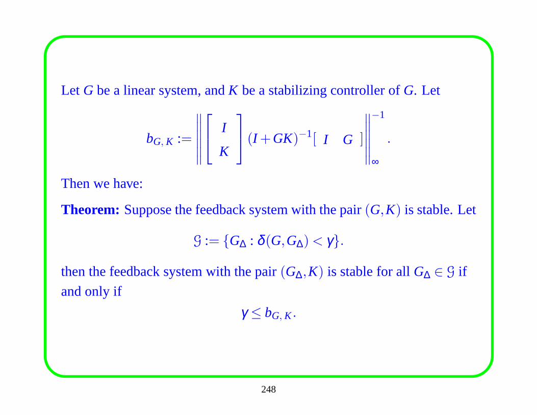
Let G be a linear system, andK be a stabilizing controller ofG. Let

bG, K :=

∥∥∥∥∥∥

I

K

(I +GK)−1[ I G ]

∥∥∥∥∥∥

−1

∞

.

Then we have:

Theorem: Suppose the feedback system with the pair(G,K) is stable. Let

G := {G∆ : δ (G,G∆)< γ}.

then the feedback system with the pair(G∆,K) is stable for allG∆ ∈ G if

and only if

γ ≤ bG, K .

248

8.2 Nonlinearity Measure

It is generally accepted that most industrial processes arenonlinear.

However, there is no definite quantification of the nonlinearity of a

process, specifically,

• How nonlinear is it?

• Can alinear controller be used to cover the whole operating range?

These are fundamental issues in the control system design. Without a

thorough understanding of the nonlinearity, the operatingrange and

performance of alinear controller cannot be guaranteed.

249

One way to approach this problem is to study the nonlinearityof a

process. The nonlinearity measure attracted much attention in the past

years, and several definitions and computation methods wereproposed.

Roughly speaking, a nonlinearity measure can be regarded asthe

‘distance’ between a nonlinear system and a class of feasible linear

systems.The first nonlinearity measure is defined as

v := infL∈Λ

‖N−L‖,

whereN is the nonlinear system considered, and the infimum is taken

over all the linear operatorsL in the feasible setΛ. The norm here can be

any appropriate norm, such asL2 or L∞. A largerv means that the system

is ‘more’ nonlinear; and in this case, a linear control may not achieve

good global performance.

250

The available nonlinearity measures have the following limitations:

1) Almost all the examples found in the literature are for SISO systems.

The computation is rather difficult for MIMO systems.

2) The available nonlinearity measures are not applicable for integrating

and unstable systems, since distances between unstable systems

cannot be measured in terms of standard norms.

A method to compute the distance between a nonlinear system and a

(fixed) linear system based on the gap metric concept was proposed. The

distance measure is closely related to nonlinearity measures in that a

nonlinearity measure computes the distance between a specified nonlinear

system and any of the feasible linear systems. So the distance measure is

the basis for computing nonlinearity measures.

251

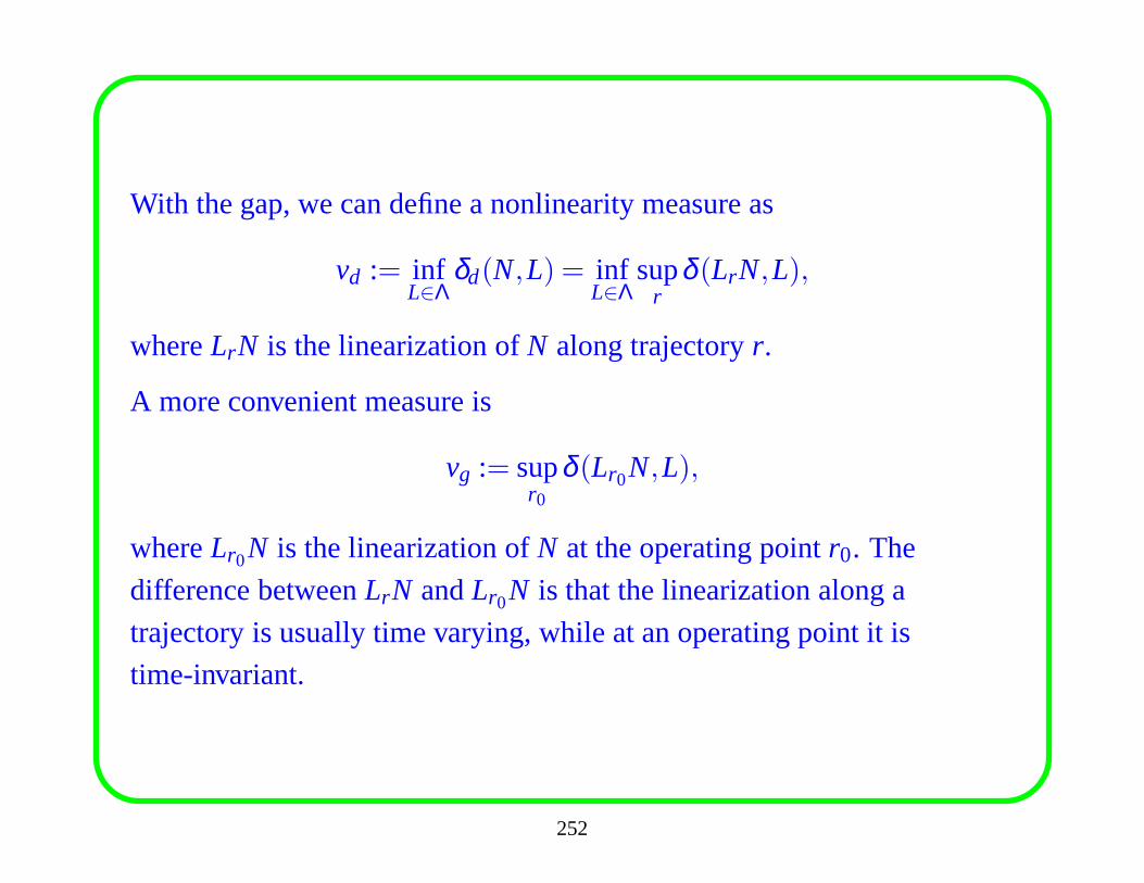
With the gap, we can define a nonlinearity measure as

vd := infL∈Λ

δd(N,L) = infL∈Λ

supr

δ (LrN,L),

whereLrN is the linearization ofN along trajectoryr.

A more convenient measure is

vg := supr0

δ (Lr0N,L),

whereLr0N is the linearization ofN at the operating pointr0. The

difference betweenLrN andLr0N is that the linearization along a

trajectory is usually time varying, while at an operating point it is

time-invariant.

252

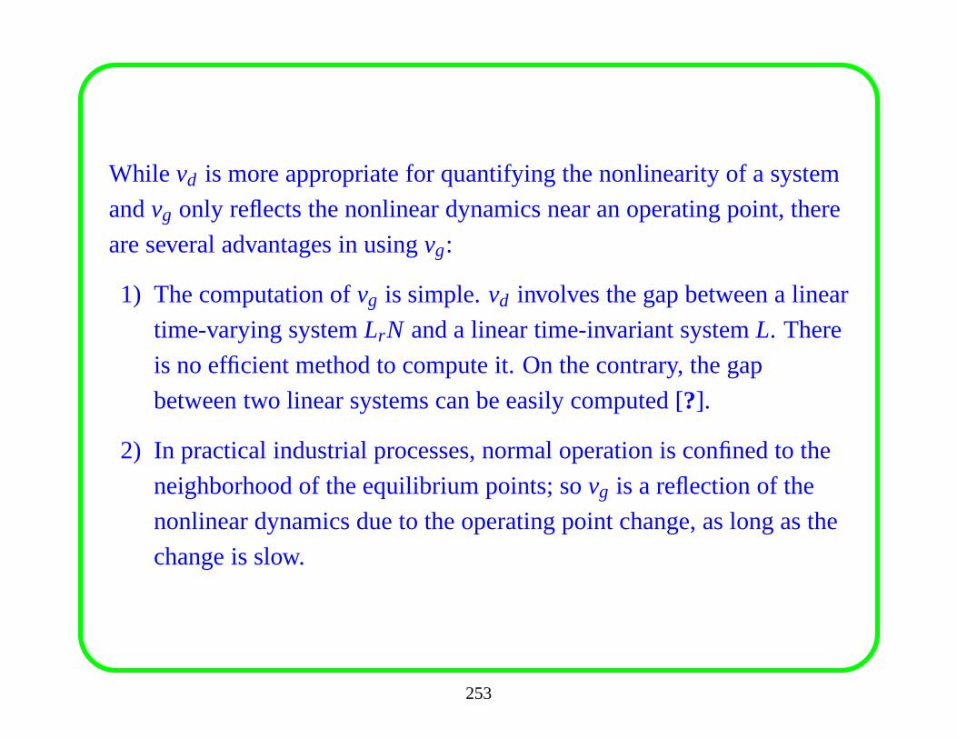
While vd is more appropriate for quantifying the nonlinearity of a system

andvg only reflects the nonlinear dynamics near an operating point, there

are several advantages in usingvg:

1) The computation ofvg is simple.vd involves the gap between a linear

time-varying systemLrN and a linear time-invariant systemL. There

is no efficient method to compute it. On the contrary, the gap

between two linear systems can be easily computed [?].

2) In practical industrial processes, normal operation is confined to the

neighborhood of the equilibrium points; sovg is a reflection of the

nonlinear dynamics due to the operating point change, as long as the

change is slow.

253

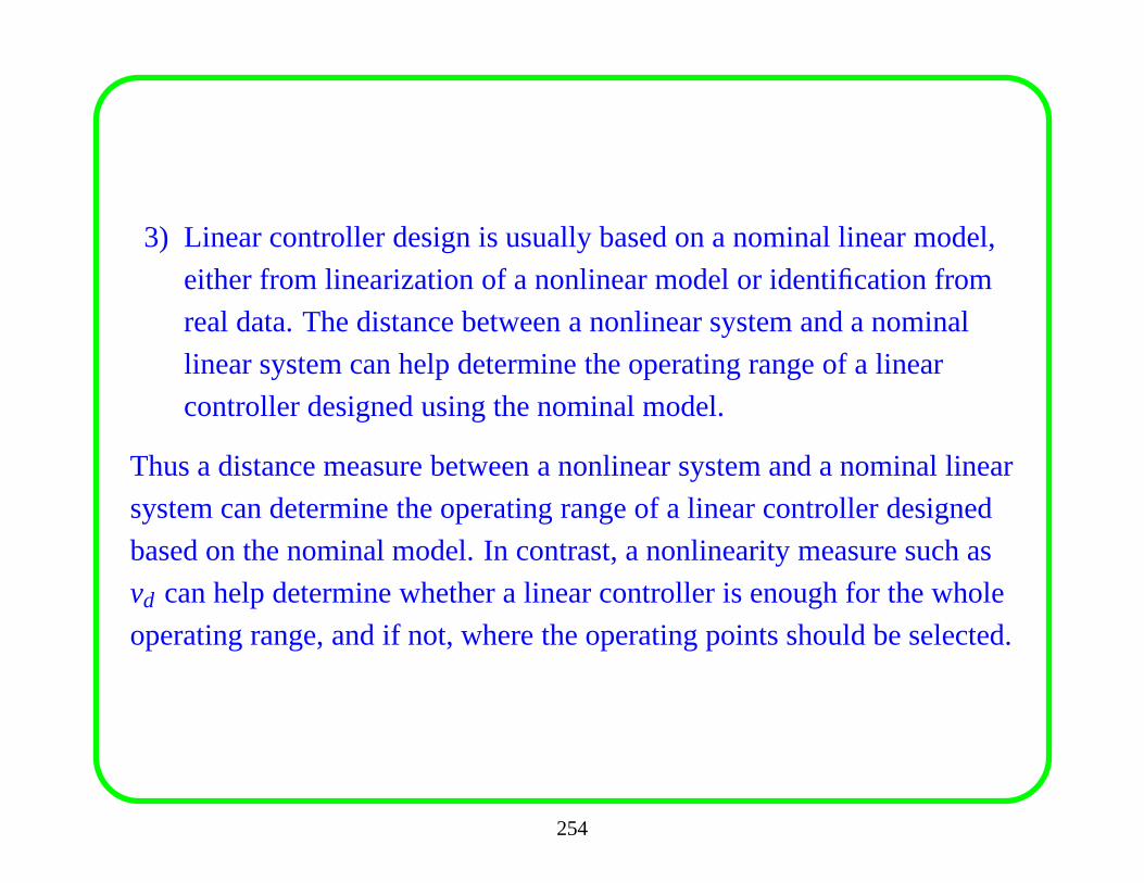
3) Linear controller design is usually based on a nominal linear model,

either from linearization of a nonlinear model or identification from

real data. The distance between a nonlinear system and a nominal

linear system can help determine the operating range of a linear

controller designed using the nominal model.

Thus a distance measure between a nonlinear system and a nominal linear

system can determine the operating range of a linear controller designed

based on the nominal model. In contrast, a nonlinearity measure such as

vd can help determine whether a linear controller is enough forthe whole

operating range, and if not, where the operating points should be selected.

254

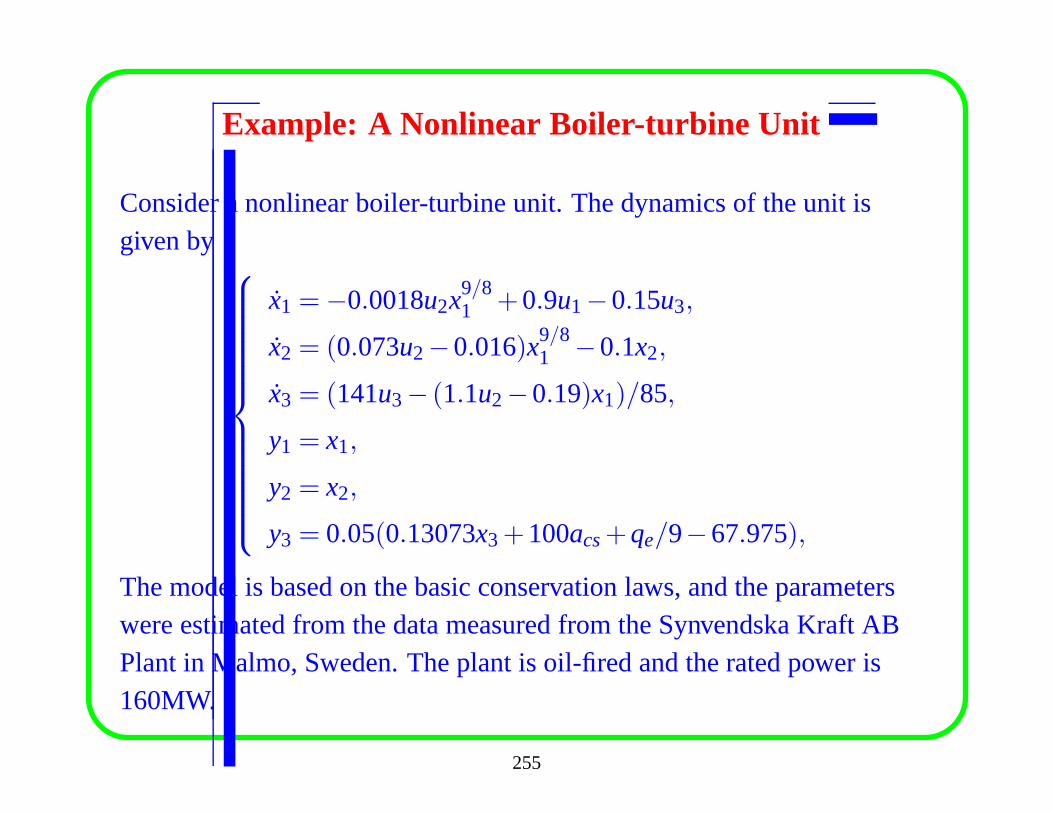
Example: A Nonlinear Boiler-turbine Unit

Consider a nonlinear boiler-turbine unit. The dynamics of the unit isgiven by

x1 =−0.0018u2x9/81 +0.9u1−0.15u3,

x2 = (0.073u2−0.016)x9/81 −0.1x2,

x3 = (141u3− (1.1u2−0.19)x1)/85,

y1 = x1,

y2 = x2,

y3 = 0.05(0.13073x3+100acs+qe/9−67.975),

The model is based on the basic conservation laws, and the parameterswere estimated from the data measured from the Synvendska Kraft ABPlant in Malmo, Sweden. The plant is oil-fired and the rated power is160MW.

255

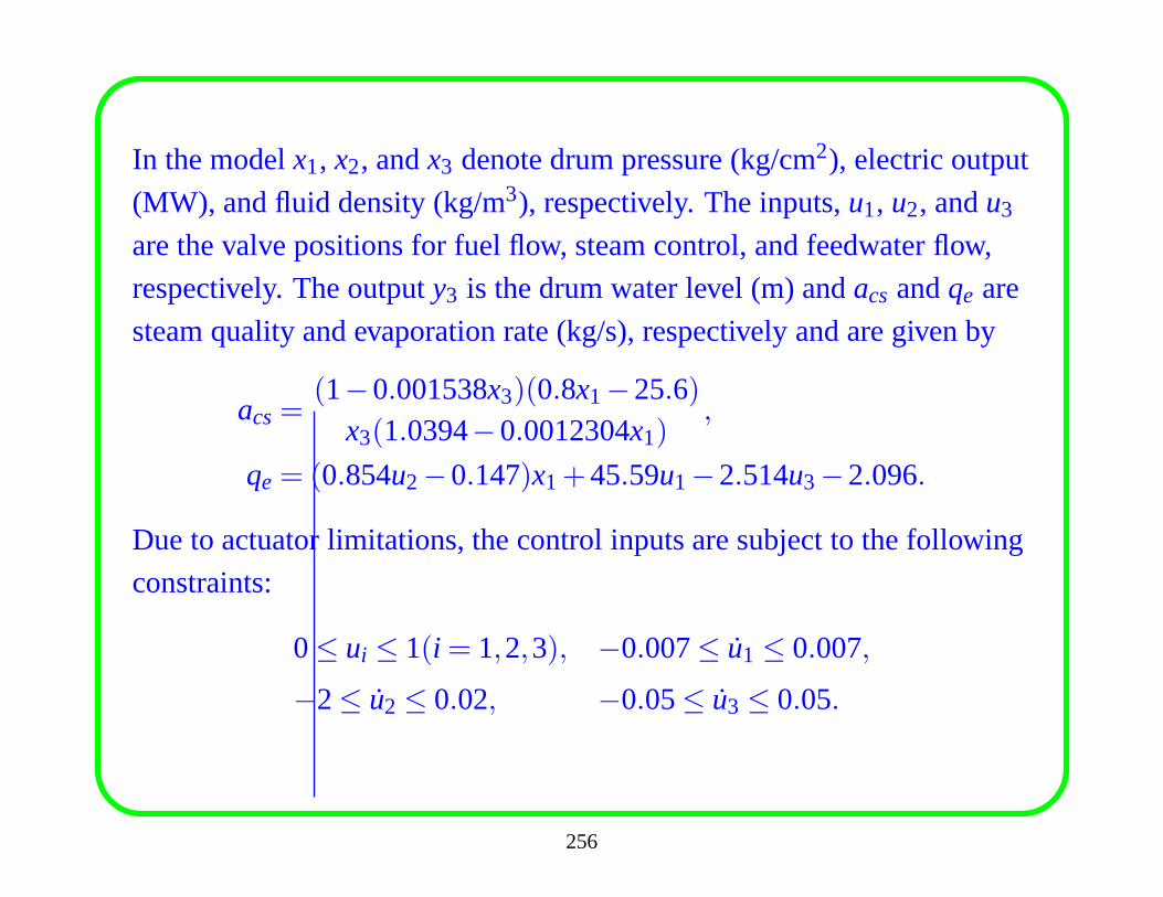
In the modelx1, x2, andx3 denote drum pressure (kg/cm2), electric output

(MW), and fluid density (kg/m3), respectively. The inputs,u1, u2, andu3

are the valve positions for fuel flow, steam control, and feedwater flow,

respectively. The outputy3 is the drum water level (m) andacs andqe are

steam quality and evaporation rate (kg/s), respectively and are given by

acs=(1−0.001538x3)(0.8x1−25.6)

x3(1.0394−0.0012304x1),

qe = (0.854u2−0.147)x1+45.59u1−2.514u3−2.096.

Due to actuator limitations, the control inputs are subjectto the following

constraints:

0≤ ui ≤ 1(i = 1,2,3), −0.007≤ u1 ≤ 0.007,

−2≤ u2 ≤ 0.02, −0.05≤ u3 ≤ 0.05.

256

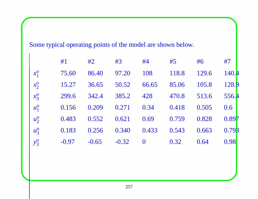
Some typical operating points of the model are shown below.

#1 #2 #3 #4 #5 #6 #7

xo1 75.60 86.40 97.20 108 118.8 129.6 140.4

xo2 15.27 36.65 50.52 66.65 85.06 105.8 128.9

xo3 299.6 342.4 385.2 428 470.8 513.6 556.4

uo1 0.156 0.209 0.271 0.34 0.418 0.505 0.6

uo2 0.483 0.552 0.621 0.69 0.759 0.828 0.897

uo3 0.183 0.256 0.340 0.433 0.543 0.663 0.793

yo3 -0.97 -0.65 -0.32 0 0.32 0.64 0.98

257

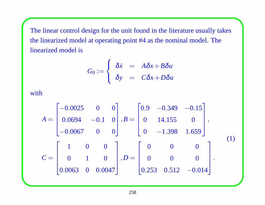
The linear control design for the unit found in the literature usually takes

the linearized model at operating point #4 as the nominal model. The

linearized model is

G0 :=

δ x = Aδx+Bδu

δy = Cδx+Dδu

with

A=

−0.0025 0 0

0.0694 −0.1 0

−0.0067 0 0

,B=

0.9 −0.349 −0.15

0 14.155 0

0 −1.398 1.659

,

C=

1 0 0

0 1 0

0.0063 0 0.0047

,D =

0 0 0

0 0 0

0.253 0.512 −0.014

.

(1)

258

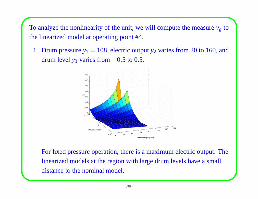
To analyze the nonlinearity of the unit, we will compute the measurevg to

the linearized model at operating point #4.

1. Drum pressurey1 = 108, electric outputy2 varies from 20 to 160, and

drum levely3 varies from−0.5 to 0.5.

−0.5

0

0.5 2040

60 80100

120 140160

0

0.1

0.2

0.3

0.4

0.5

0.6

0.7

Electric Output (MW)

Drume Level (m)

v g

For fixed pressure operation, there is a maximum electric output. The

linearized models at the region with large drum levels have asmall

distance to the nominal model.

259

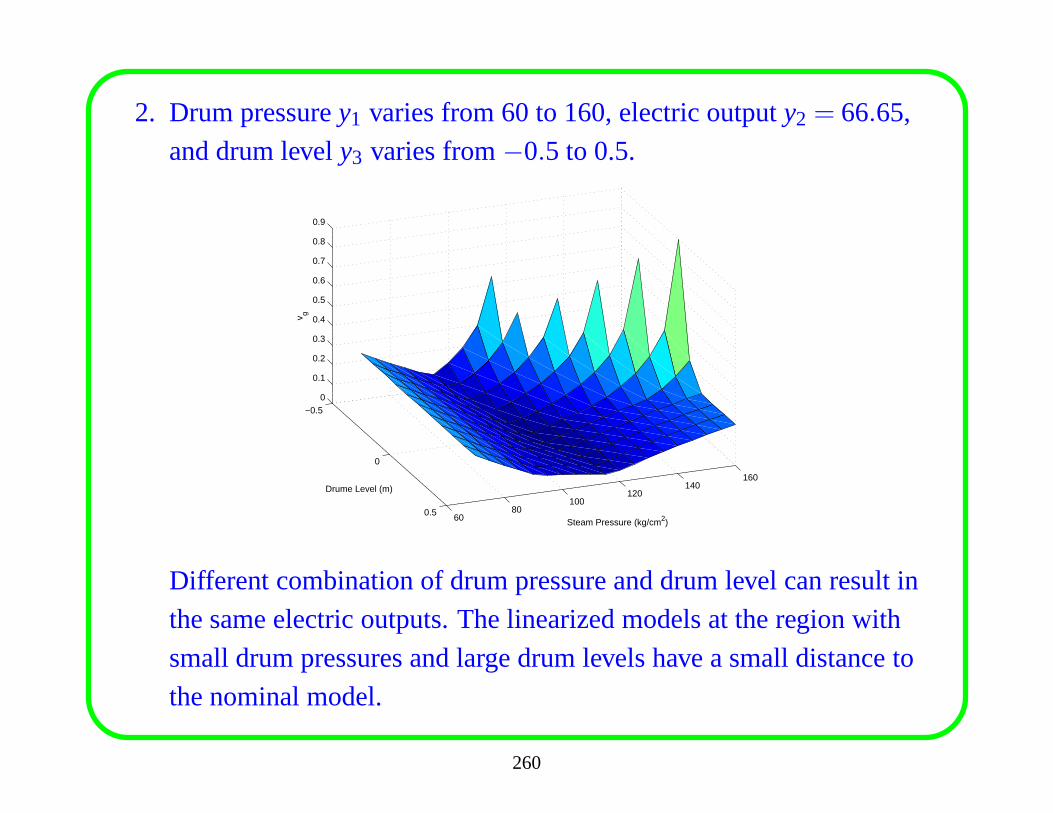
2. Drum pressurey1 varies from 60 to 160, electric outputy2 = 66.65,

and drum levely3 varies from−0.5 to 0.5.

−0.5

0

0.5 6080

100120

140160

0

0.1

0.2

0.3

0.4

0.5

0.6

0.7

0.8

0.9

Steam Pressure (kg/cm2)

Drume Level (m)

v g

Different combination of drum pressure and drum level can result in

the same electric outputs. The linearized models at the region with

small drum pressures and large drum levels have a small distance to

the nominal model.

260

3. Drum pressurey1 varies from 60 to 160, electric outputy2 varies

from 20 to 160, and drum levely3 = 0.

20

40

60

80

100

120

60

80

100

120

140

1600

0.2

0.4

0.6

0.8

Electric Output (MW)Steam Pressure (kg/cm2)

v g

For fixed drum level operation, only the linearized models atthe region

with small electric outputs have a small distance to the nominal model.

261

It is also observed

• Larger values ofvg occur at the region with large drum pressures,

large electric outputs, and small drum levels; The maximum is about

0.9.

To evaluate the nonlinearity of the unit, we need to computevg by taking

L as linearized models at other operating points. It is found that the

maximum ofvg is always larger than 0.7, so we conclude that the Bell and

Astrom model shows severe nonlinearity.

262

8.3 Linear Control of Nonlinear Processes

If a process shows severe nonlinearity, does it mean that only nonlinearcontrollers can be used to achieve wide-range performance?The answeris NO.

In this section we will show that by careful choice of operation points thecontrol system can avoid the nonlinearity and a linear controller is enoughin the operating range.

Example: (continue)

The plots ofvg show us how to ‘avoid’ the nonlinear dynamics due to theoperating point change. Since a boiler-turbine unit must follow theelectricity demand from the grid, and the same amount of electric outputcan be obtained with different combination of drum pressureand drumlevel, the operating range of the unit should be carefully chosen.

263

For instant, if a linear controller is designed at operatingpoint #4, then we

should avoid driving the unit to operating points that have large drum

pressures, large electric outputs, and small drum levels, since at these

operating points the dynamics are quite different from the nominal one.

A good operation is to increase the drum pressure and drum level as the

electric output is increased. In this case the dynamics at the operating

region will not be far away from the nominal, thus stability of the system

can be guaranteed.

To verify the argument, we compute the gaps between the linearized

models at the typical operating points. It is clear that the gaps between

them are small, the largest being between models at operating point #1

and #7. If the nominal model is taken at #4, then as long as the designed

linear controllerK satisfiesbG,K > 0.195, then the controller can

guarantee the closed-loop stability at other operating points.

264

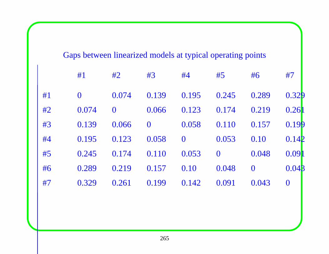
Gaps between linearized models at typical operating points

#1 #2 #3 #4 #5 #6 #7

#1 0 0.074 0.139 0.195 0.245 0.289 0.329

#2 0.074 0 0.066 0.123 0.174 0.219 0.261

#3 0.139 0.066 0 0.058 0.110 0.157 0.199

#4 0.195 0.123 0.058 0 0.053 0.10 0.142

#5 0.245 0.174 0.110 0.053 0 0.048 0.091

#6 0.289 0.219 0.157 0.10 0.048 0 0.043

#7 0.329 0.261 0.199 0.142 0.091 0.043 0

265

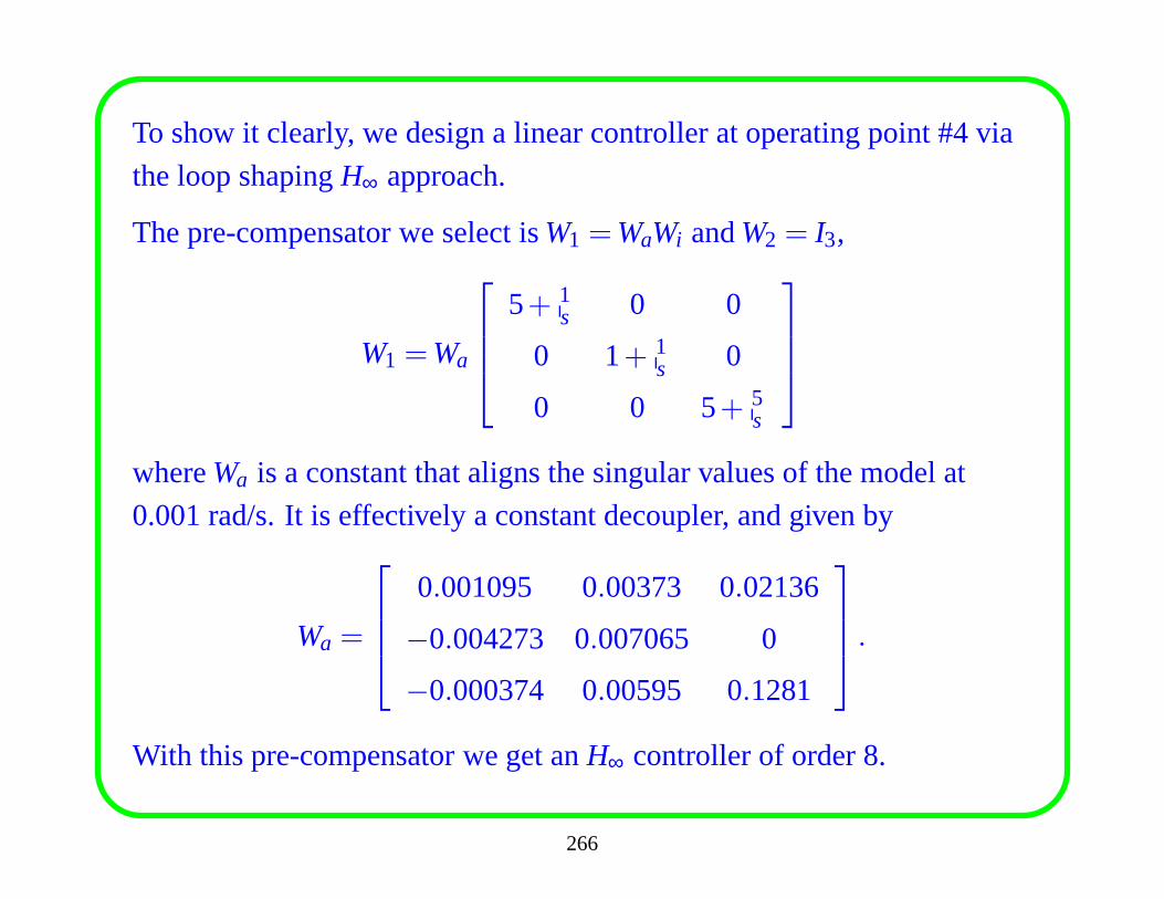
To show it clearly, we design a linear controller at operating point #4 via

the loop shapingH∞ approach.

The pre-compensator we select isW1 =WaWi andW2 = I3,

W1 =Wa

5+ 1s 0 0

0 1+ 1s 0

0 0 5+ 5s

whereWa is a constant that aligns the singular values of the model at

0.001 rad/s. It is effectively a constant decoupler, and given by

Wa =

0.001095 0.00373 0.02136

−0.004273 0.007065 0

−0.000374 0.00595 0.1281

.

With this pre-compensator we get anH∞ controller of order 8.

266

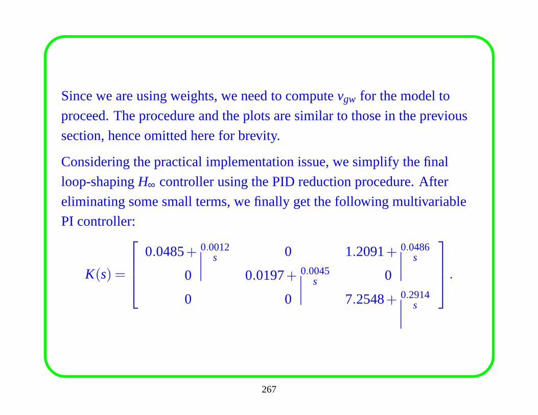
Since we are using weights, we need to computevgw for the model to

proceed. The procedure and the plots are similar to those in the previous

section, hence omitted here for brevity.

Considering the practical implementation issue, we simplify the final

loop-shapingH∞ controller using the PID reduction procedure. After

eliminating some small terms, we finally get the following multivariable

PI controller:

K(s) =

0.0485+ 0.0012s 0 1.2091+ 0.0486

s

0 0.0197+ 0.0045s 0

0 0 7.2548+ 0.2914s

.

267

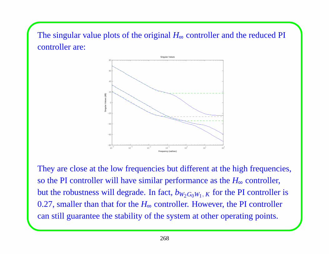
The singular value plots of the originalH∞ controller and the reduced PIcontroller are:

10−4

10−3

10−2

10−1

100

101

102

−80

−60

−40

−20

0

20

40

60

80

Singular Values

Frequency (rad/sec)

Sin

gula

r V

alue

s (d

B)

They are close at the low frequencies but different at the high frequencies,so the PI controller will have similar performance as theH∞ controller,but the robustness will degrade. In fact,bW2G0W1, K for the PI controller is0.27, smaller than that for theH∞ controller. However, the PI controllercan still guarantee the stability of the system at other operating points.

268

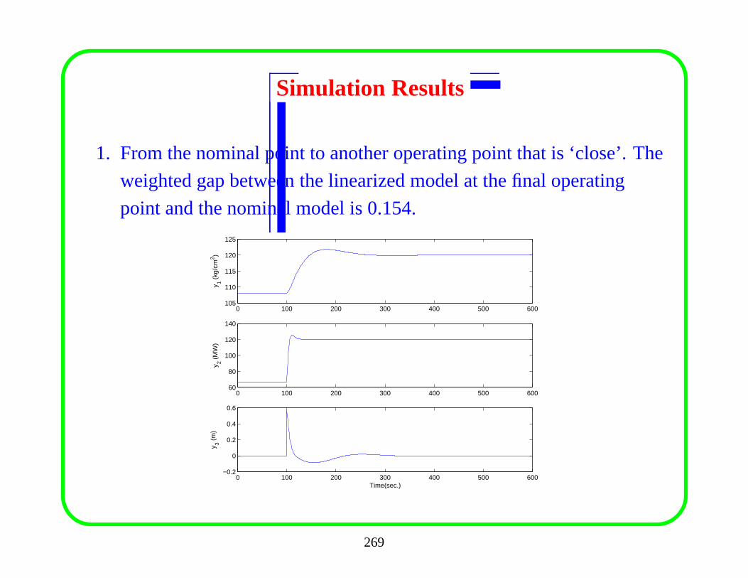
Simulation Results

1. From the nominal point to another operating point that is ‘close’. The

weighted gap between the linearized model at the final operating

point and the nominal model is 0.154.

0 100 200 300 400 500 600105

110

115

120

125

y 1 (kg

/cm

2 )

0 100 200 300 400 500 60060

80

100

120

140

y 2 (M

W)

0 100 200 300 400 500 600−0.2

0

0.2

0.4

0.6

y 3 (m

)

Time(sec.)

269

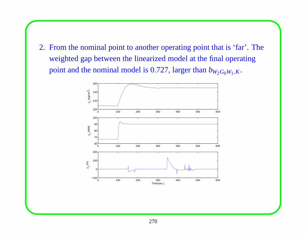
2. From the nominal point to another operating point that is ‘far’. The

weighted gap between the linearized model at the final operating

point and the nominal model is 0.727, larger thanbW2G0W1,K .

0 100 200 300 400 500 600100

120

140

160

y 1 (kg

/cm

2 )

0 100 200 300 400 500 60060

70

80

90

100

y 2 (M

W)

0 100 200 300 400 500 600−100

0

100

200

y 3 (m

)

Time(sec.)

270

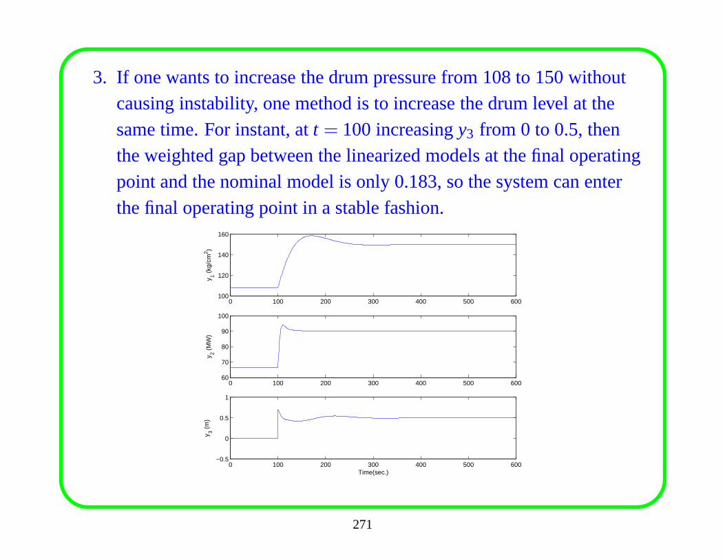
3. If one wants to increase the drum pressure from 108 to 150 withoutcausing instability, one method is to increase the drum level at thesame time. For instant, att = 100 increasingy3 from 0 to 0.5, thenthe weighted gap between the linearized models at the final operatingpoint and the nominal model is only 0.183, so the system can enterthe final operating point in a stable fashion.

0 100 200 300 400 500 600100

120

140

160

y 1 (kg

/cm

2 )

0 100 200 300 400 500 60060

70

80

90

100

y 2 (M

W)

0 100 200 300 400 500 600−0.5

0

0.5

1

y 3 (m

)

Time(sec.)

271

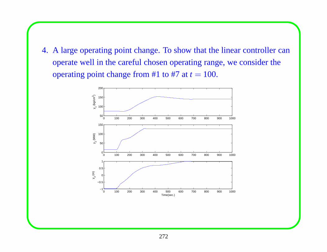
4. A large operating point change. To show that the linear controller can

operate well in the careful chosen operating range, we consider the

operating point change from #1 to #7 att = 100.

0 100 200 300 400 500 600 700 800 900 100050

100

150

200

y 1 (kg

/cm

2 )

0 100 200 300 400 500 600 700 800 900 10000

50

100

150

y 2 (M

W)

0 100 200 300 400 500 600 700 800 900 1000−1

−0.5

0

0.5

1

y 3 (m

)

Time(sec.)

272

8.4 Multimodel Control

If a single linear controller cannot achieve the performance in the desiredrange for a nonlinear system, then nonlinear strategies should beconsidered. The simplest method is the so called ’multimodel control’.The method represents the nonlinear system as a combinationof linearsystems.

Several problems are critical for multimodel control:

1) How many models are sufficient in design? Where the models shouldbe selected?

2) How to combine local controllers? Switching or weighting?

3) How to prove that the performance can be guaranteed for themultimodel controller?

These problems are not yet completely solved.

273

Selection of Operating Points

Gap metric is suggested as a guideline for selecting local models. The

idea is that the ‘distance’ of two selected models should notbe larger than

a prescribed level. Since local controller can be designed to robustly

stabilize all the models within the prescribed level, models selected in this

way can guarantee the global stability of the closed-loop systems as long

as the change of models is ‘slow’.

Theoretical background in applying the gap metric in selecting operating

points for multimodel controller design is Theorem ?. It shows that a

linear controllerK can stabilize all the linear systems that have a distance

to G less thanbG, K .

274

Suppose now a certain operating point has been selected. Thelocal model

is G and the local controller isK. Then the next operating point should be

selected at a distance (in the gap metric sense) no larger than bG, K , since

all models with a gap metric less thanbG, K to the given model can be

stabilized by the local controllerK. To have a minimal set of the

operating points, the next operating point should be selected at a distance

exactly equal tobG, K , or just a little smaller than it.

In practice, the local controller is not available before selecting the

operating points, so we can first prescribe a distance level,and then

starting from an initial operating point, compute the next operating point

till the whole range of the operating points are covered.

275

There are two drawbacks when applying the gap metric in selecting the

operating points for multimodel controller design:

1) The gap metric is only related to robust stability, that is, the local

controllerK can only guarantee that it can stabilize the models at

operating points close to the given operating point. However, stability

is not the only issue in control system design. Other performance

should also be guaranteed in selecting operating points.

2) In multimodel controller design,bG, K should be checked to make

sure it is larger than the prescribed distance level, otherwise robust

stability cannot be guaranteed.

276

Motivated by the loop shapingH∞ approach, we can include performance

weights in the gap metric computation.

Since

bopt = maxK

bG, K

Sobopt is the maximum of the robustness margin for the shaped plantG,

and we can directly obtainbopt with loop shapingH∞ design.

The gap metric between the shaped plants thus has potential applications

in selecting operating points for multimodel controller design. We

compute the distance between the shaped models instead of the original

models. Then a shaped model with a distance less thanbopt to a given

(shaped) model at one operating point can be stabilized withthe local

optimal controller and the performance can be guaranteed.

277

Multimodel Controller Design

The procedure of multimodel controller design goes as follows:

1. Compensator selection for performance. We have discussed some

guidelines in choosing the pre- and/or post-compensators to reflect

the performance requirements. However, for multimodel controller

design, we have two options in choosing the compensators:

(a) Choose a fixed set of pre- and/or post-compensators for all

operating points.

(b) Choose different sets of pre- and/or post-compensatorsat

different operating points.

278

Obviously, the first method is simple. However, due to different gains

of the models at different operating points, the resulting open-loop

shapes will certainly be different, that means at differentoperating

points the performance specifications are different, whichis

undesired.

The most desired is that at all the operating points, we specify the

same open-loop shapes. However, it is not always possible due to

system nonlinearity. Note that in process control most of the

disturbance arises at the low frequency, so we will choose sets of

compensators such that the desired open-loop shapes at all operating

points are almost the same at the low frequency, which means that the

closed-loop systems will have similar disturbance rejection ability at

all operating points.

279

2. Local controller design. It is a standard practice to design such loop

shaping controllers. One thing to remember is to check whether the

designedbG,K is actually less thanbopt, otherwise the operating

points selected are not appropriate and new operating points needed

to be re-selected.

3. Constructing the multimodel controller. Once local controllers are

designed, we can form the global controller by switching, orusing

weights (fuzzy logic). We will use membership functions to create a

transition region according to the operating pointz,

u(t) =k

∑i=1

ui(t)ρi(z)

wherek is the number of operating points,ui(t) is the output of the

ith local controller, andρi(z) is the membership function of theith

local controller.

280

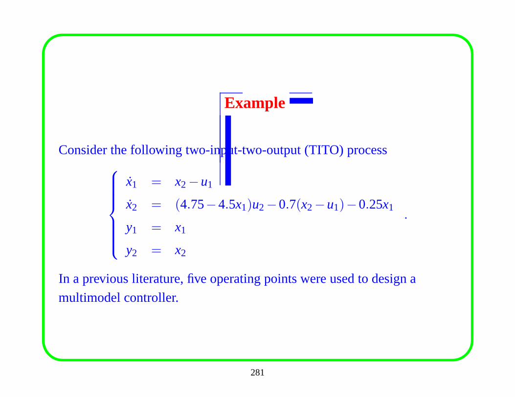
Example

Consider the following two-input-two-output (TITO) process

x1 = x2−u1

x2 = (4.75−4.5x1)u2−0.7(x2−u1)−0.25x1

y1 = x1

y2 = x2

.

In a previous literature, five operating points were used to design a

multimodel controller.

281

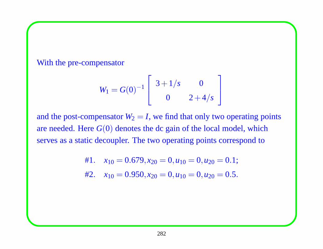
With the pre-compensator

W1 = G(0)−1

3+1/s 0

0 2+4/s

and the post-compensatorW2 = I , we find that only two operating points

are needed. HereG(0) denotes the dc gain of the local model, which

serves as a static decoupler. The two operating points correspond to

#1. x10 = 0.679,x20 = 0,u10 = 0,u20 = 0.1;

#2. x10 = 0.950,x20 = 0,u10 = 0,u20 = 0.5.

282

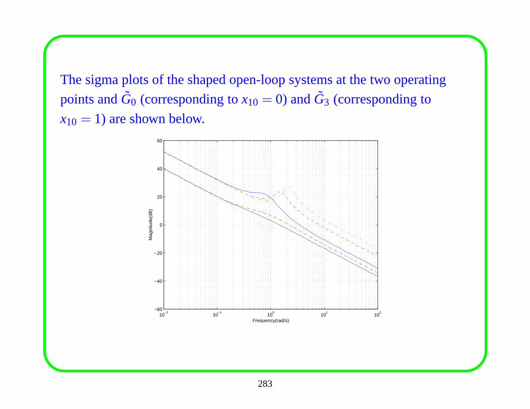
The sigma plots of the shaped open-loop systems at the two operating

points andG0 (corresponding tox10 = 0) andG3 (corresponding to

x10 = 1) are shown below.

10−2

10−1

100

101

102

−60

−40

−20

0

20

40

60

Frequency(rad/s)

Mag

nitu

de(d

B)

283

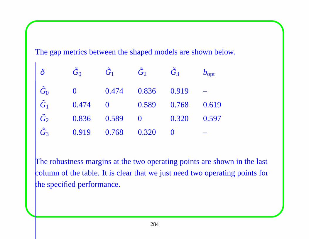
The gap metrics between the shaped models are shown below.

δ G0 G1 G2 G3 bopt

G0 0 0.474 0.836 0.919 –

G1 0.474 0 0.589 0.768 0.619

G2 0.836 0.589 0 0.320 0.597

G3 0.919 0.768 0.320 0 –

The robustness margins at the two operating points are shownin the last

column of the table. It is clear that we just need two operating points for

the specified performance.

284

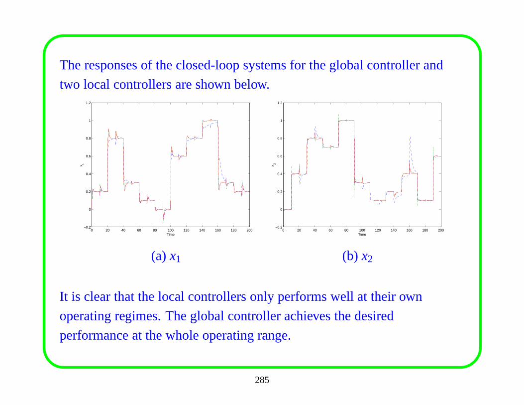
The responses of the closed-loop systems for the global controller and

two local controllers are shown below.

0 20 40 60 80 100 120 140 160 180 200−0.2

0

0.2

0.4

0.6

0.8

1

1.2

Time

x 1

0 20 40 60 80 100 120 140 160 180 200−0.2

0

0.2

0.4

0.6

0.8

1

1.2

Time

x 2

(a) x1 (b) x2

It is clear that the local controllers only performs well at their own

operating regimes. The global controller achieves the desired

performance at the whole operating range.

285