Robust Control of an Inverted Pendulum on a Cart€¦ · Robust Control of an Inverted Pendulum on...
16
Robust Control of an Inverted Pendulum on a Cart Alexis Ball ME/ECE 854 Robust Control Final Project Due: April 29, 2007 Abstract This paper investigates the design and analysis of three controllers used to stabilize an inverted pendulum on a cart. This is accomplished by decomposing each control algorithm into two separate phases: swing-up control and stabilization control. A classical, H 2 , and H ∞ design are each considered to stabilize a nominal linearized model of the inverted pendulum on a cart in the upward vertical position. The effectiveness of each stabilizing design is evaluated through the use of the μ synthesis bound, as it applies to nominal performance, robust stability, and robust performance. Simulation results are provided to show the validity of each method. I. INTRODUCTION The inverted pendulum is a canonical example of a nonlinear system. The dynamics inherent in the model are often used to represent problems dealing with balance, such as bipedal walking as explored in [1], [2], and [3], unicycles [4], and the Segway Personal Transporters [5], due to the inherent instability of the system. Moreover, the inverted pendulum on a cart is often viewed as an under-actuated mechanical system, where the control inputs available are less than the degrees of freedom of the system. Thus, the natural complexity of this deceptively simple system makes it a prime candidate as a baseline study when investigating new control algorithms. However, as with all systems, the models are never perfect. Thus, with the addition of model uncertainty paired with sensor noise and other unknown exogenous disturbances, the system previously thought to be stabilized can easily go unstable. The authors of [6] attempt to address the variability in system representation through the design of a controller using neutral networks. Although the approach is successful, no consideration is given to the possibility of outside disturbances. In [7], parametric uncertainties are dealt with via a combination of classic control theory and grey theory. In particular, the authors use a grey prediction model combined with a proportional plus derivative controller to balanced the inverted pendulum. Yet, the information received from the sensors is assumed to be flawless. Note that there are other possible methods and approaches that may be used to control an inverted pendulum, with
Transcript of Robust Control of an Inverted Pendulum on a Cart€¦ · Robust Control of an Inverted Pendulum on...
Robust Control of an Inverted Pendulum on a Cart
Alexis Ball
ME/ECE 854 Robust Control
Final Project
Due: April 29, 2007
Abstract
This paper investigates the design and analysis of three controllers used to stabilize an inverted pendulum
on a cart. This is accomplished by decomposing each control algorithm into two separate phases: swing-up
control and stabilization control. A classical, H2, and H∞ design are each considered to stabilize a nominal
linearized model of the inverted pendulum on a cart in the upward vertical position. The effectiveness of
each stabilizing design is evaluated through the use of the µ synthesis bound, as it applies to nominal
performance, robust stability, and robust performance. Simulation results are provided to show the validity
of each method.
I. INTRODUCTION
The inverted pendulum is a canonical example of a nonlinear system. The dynamics inherent in the
model are often used to represent problems dealing with balance, such as bipedal walking as explored in
[1], [2], and [3], unicycles [4], and the Segway Personal Transporters [5], due to the inherent instability of
the system. Moreover, the inverted pendulum on a cart is often viewed as an under-actuated mechanical
system, where the control inputs available are less than the degrees of freedom of the system. Thus, the
natural complexity of this deceptively simple system makes it a prime candidate as a baseline study when
investigating new control algorithms.
However, as with all systems, the models are never perfect. Thus, with the addition of model
uncertainty paired with sensor noise and other unknown exogenous disturbances, the system previously
thought to be stabilized can easily go unstable. The authors of [6] attempt to address the variability in
system representation through the design of a controller using neutral networks. Although the approach
is successful, no consideration is given to the possibility of outside disturbances. In [7], parametric
uncertainties are dealt with via a combination of classic control theory and grey theory. In particular, the
authors use a grey prediction model combined with a proportional plus derivative controller to balanced
the inverted pendulum. Yet, the information received from the sensors is assumed to be flawless. Note that
there are other possible methods and approaches that may be used to control an inverted pendulum, with
only a select few mentioned in this work. Moreover, the mathematical model and physical system itself
can also vary widely in the literature.
The goal of this body of work is to study the inverted pendulum on a cart within the context of model
uncertainty, sensor noise, and external disturbances, and provide a comparison between pole-placement,
H2, and H∞ design methods as they relate to the overall system stability and performance. Section 2
fleshes out the details pertaining to the physical and mathematical description of the pendulum model used
in this study. This includes the error introduced into the model through the linearization of the nonlinear
system. The idea behind the use of two separate control algorithms and system representations to swing-up
the pendulum from rest to an upright position is addressed in Section 3; in particular, there is a swing-up
controller to be used initially and a stabilization controller to help maintain the pendulum at the vertical
upright position. Given the swing-up period is not the focus of this paper (requires no robust control
methods), the method will not be explored beyond Section 3. A entire section, Section 4, is dedicated
to providing the technical details relevant to the three separate methods used for stabilization, including
supplying the system form that lends itself to the robust control approach, performance requirements, and
the design methodology. Some preliminary closed-loop system results are provided, but not fully quantified
until Section 5. The success in terms of nominal performance, robust stability, and robust performance are
addressed using µ synthesis in Section 5. An overall comparison between the three methods is also given.
II. PROBLEM FORMULATION AND SYSTEM DESCRIPTION
The system of interest is an inverted pendulum mounted on a motor driven cart. The rod mounted on
the cart is “free-moving” in the sense that there are no actuators dedicated to moving the pendulum alone.
Furthermore, both the cart and the pendulum are constrained to movement within the vertical plane. Any
movement that is experienced by the pendulum must be due to movement induced by the cart; this may
include outside disturbances such as wind or human interference (such as pushing the pendulum or cart) in
addition to the motion generated by the motors. However, all disturbances entering the system are assumed
to be bounded and have finite energy. This fact will later be utilized when designing the robust portion of
the control algorithm, such that all disturbances fit into a set of L2 disturbances (to be defined).
Using simple Newtonian physics and the free body diagrams shown in Fig. 1, we can begin to define
the dynamics of the inverted pendulum on a cart. It is assumed that the mass of the cart is M = 0.5kg and
the mass of the pendulum m = 0.5kg. The cart is subjected to a frictional force, where the coefficient of
friction is represented as b = 0.1N/m/sec. Naturally, this force is assumed to be in the opposite direction
of the applied force on the cart. The externally applied force F is assumed to be composed of the control
input and the external disturbances acting on the cart. The length of the pendulum to the center of the
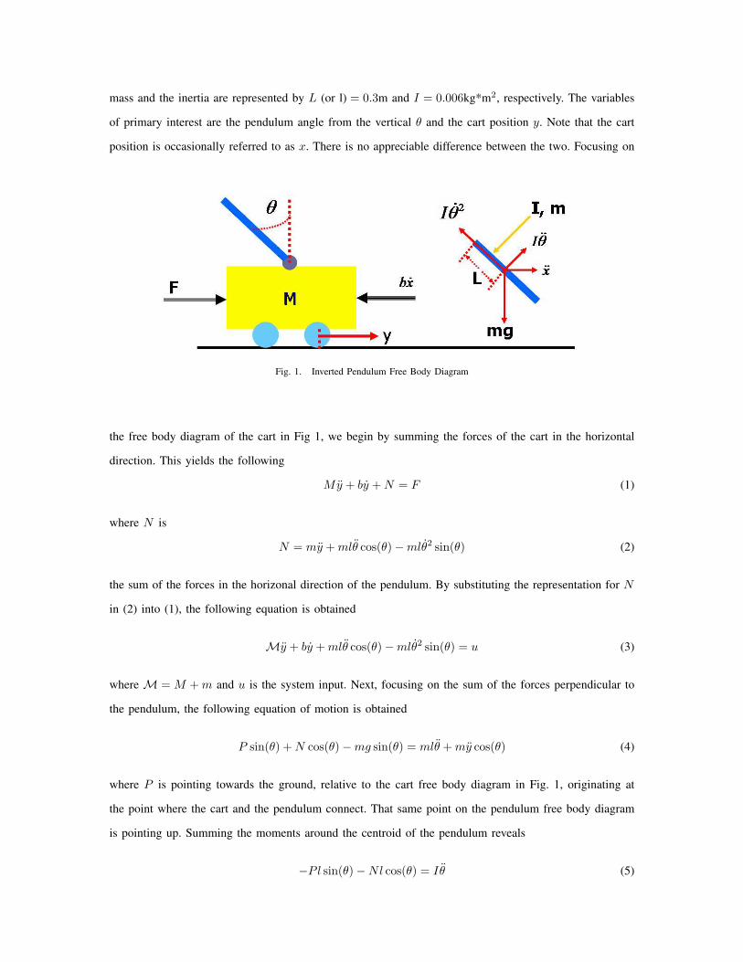
mass and the inertia are represented by L (or l) = 0.3m and I = 0.006kg*m2, respectively. The variables
of primary interest are the pendulum angle from the vertical θ and the cart position y. Note that the cart
position is occasionally referred to as x. There is no appreciable difference between the two. Focusing on
Fig. 1. Inverted Pendulum Free Body Diagram
the free body diagram of the cart in Fig 1, we begin by summing the forces of the cart in the horizontal
direction. This yields the following
My + by + N = F (1)
where N is
N = my + mlθ cos(θ)−mlθ2 sin(θ) (2)
the sum of the forces in the horizonal direction of the pendulum. By substituting the representation for N
in (2) into (1), the following equation is obtained
My + by + mlθ cos(θ)−mlθ2 sin(θ) = u (3)
where M = M + m and u is the system input. Next, focusing on the sum of the forces perpendicular to
the pendulum, the following equation of motion is obtained
P sin(θ) + N cos(θ)−mg sin(θ) = mlθ + my cos(θ) (4)
where P is pointing towards the ground, relative to the cart free body diagram in Fig. 1, originating at
the point where the cart and the pendulum connect. That same point on the pendulum free body diagram
is pointing up. Summing the moments around the centroid of the pendulum reveals
−Pl sin(θ)−Nl cos(θ) = Iθ (5)
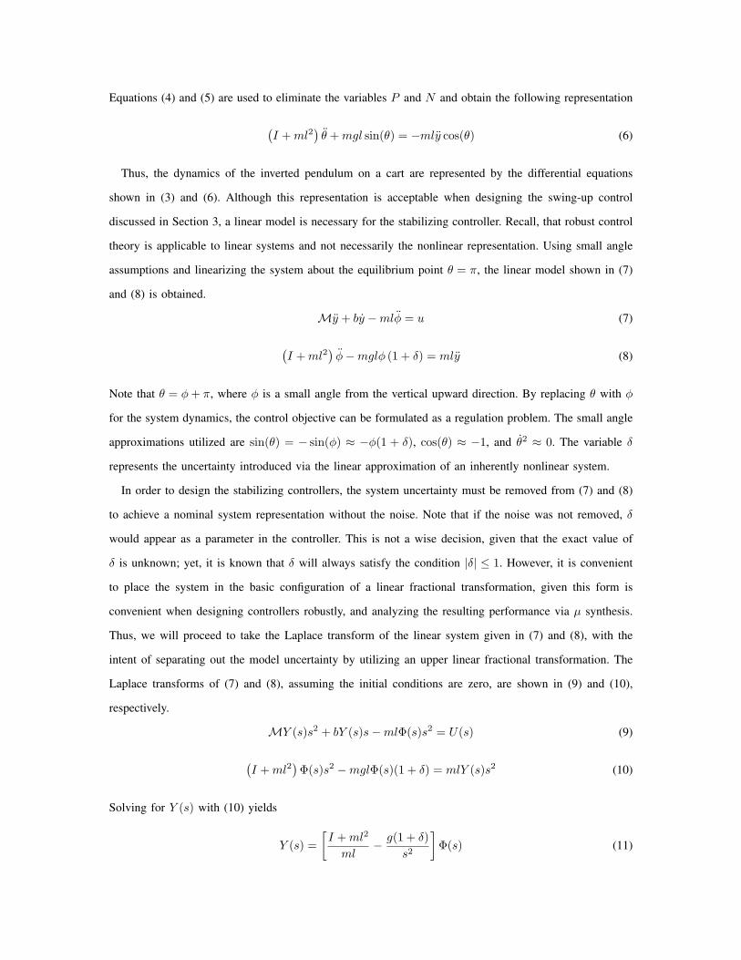
Equations (4) and (5) are used to eliminate the variables P and N and obtain the following representation
(I + ml2
)θ + mgl sin(θ) = −mly cos(θ) (6)
Thus, the dynamics of the inverted pendulum on a cart are represented by the differential equations
shown in (3) and (6). Although this representation is acceptable when designing the swing-up control
discussed in Section 3, a linear model is necessary for the stabilizing controller. Recall, that robust control
theory is applicable to linear systems and not necessarily the nonlinear representation. Using small angle
assumptions and linearizing the system about the equilibrium point θ = π, the linear model shown in (7)
and (8) is obtained.
My + by −mlφ = u (7)
(I + ml2
)φ−mglφ (1 + δ) = mly (8)
Note that θ = φ + π, where φ is a small angle from the vertical upward direction. By replacing θ with φ
for the system dynamics, the control objective can be formulated as a regulation problem. The small angle
approximations utilized are sin(θ) = − sin(φ) ≈ −φ(1 + δ), cos(θ) ≈ −1, and θ2 ≈ 0. The variable δ
represents the uncertainty introduced via the linear approximation of an inherently nonlinear system.
In order to design the stabilizing controllers, the system uncertainty must be removed from (7) and (8)
to achieve a nominal system representation without the noise. Note that if the noise was not removed, δ
would appear as a parameter in the controller. This is not a wise decision, given that the exact value of
δ is unknown; yet, it is known that δ will always satisfy the condition |δ| ≤ 1. However, it is convenient
to place the system in the basic configuration of a linear fractional transformation, given this form is
convenient when designing controllers robustly, and analyzing the resulting performance via µ synthesis.
Thus, we will proceed to take the Laplace transform of the linear system given in (7) and (8), with the
intent of separating out the model uncertainty by utilizing an upper linear fractional transformation. The
Laplace transforms of (7) and (8), assuming the initial conditions are zero, are shown in (9) and (10),
respectively.
MY (s)s2 + bY (s)s−mlΦ(s)s2 = U(s) (9)
(I + ml2
)Φ(s)s2 −mglΦ(s)(1 + δ) = mlY (s)s2 (10)
Solving for Y (s) with (10) yields
Y (s) =[I + ml2
ml− g(1 + δ)
s2
]Φ(s) (11)
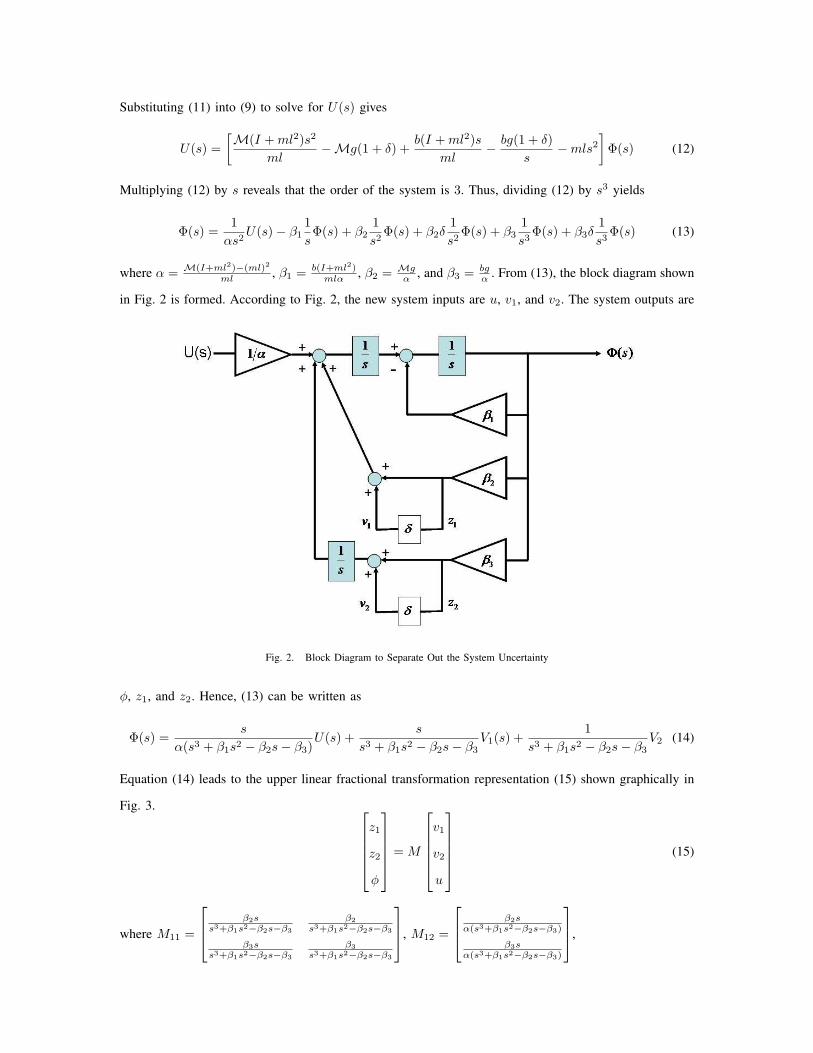
Substituting (11) into (9) to solve for U(s) gives
U(s) =[M(I + ml2)s2
ml−Mg(1 + δ) +
b(I + ml2)sml
− bg(1 + δ)s
−mls2
]Φ(s) (12)
Multiplying (12) by s reveals that the order of the system is 3. Thus, dividing (12) by s3 yields
Φ(s) =1
αs2U(s)− β1
1sΦ(s) + β2
1s2
Φ(s) + β2δ1s2
Φ(s) + β31s3
Φ(s) + β3δ1s3
Φ(s) (13)
where α = M(I+ml2)−(ml)2
ml , β1 = b(I+ml2)mlα , β2 = Mg
α , and β3 = bgα . From (13), the block diagram shown
in Fig. 2 is formed. According to Fig. 2, the new system inputs are u, v1, and v2. The system outputs are
Fig. 2. Block Diagram to Separate Out the System Uncertainty
φ, z1, and z2. Hence, (13) can be written as
Φ(s) =s
α(s3 + β1s2 − β2s− β3)U(s) +
s
s3 + β1s2 − β2s− β3V1(s) +
1s3 + β1s2 − β2s− β3
V2 (14)
Equation (14) leads to the upper linear fractional transformation representation (15) shown graphically in
Fig. 3.
z1
z2
φ
= M
v1
v2
u
(15)
where M11 =
β2ss3+β1s2−β2s−β3
β2s3+β1s2−β2s−β3
β3ss3+β1s2−β2s−β3
β3s3+β1s2−β2s−β3
, M12 =
β2sα(s3+β1s2−β2s−β3)
β3sα(s3+β1s2−β2s−β3)
,
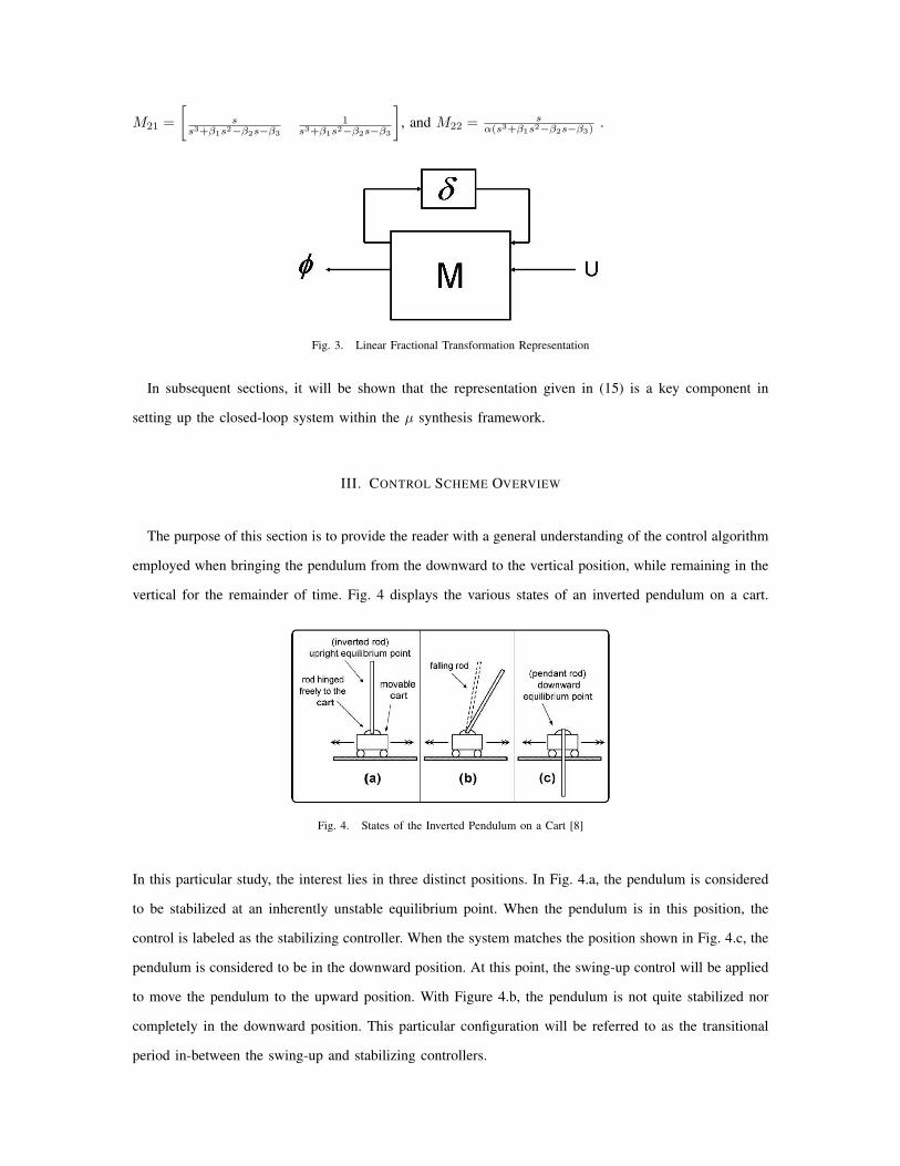
M21 =[
ss3+β1s2−β2s−β3
1s3+β1s2−β2s−β3
], and M22 = s
α(s3+β1s2−β2s−β3).
Fig. 3. Linear Fractional Transformation Representation
In subsequent sections, it will be shown that the representation given in (15) is a key component in
setting up the closed-loop system within the µ synthesis framework.
III. CONTROL SCHEME OVERVIEW
The purpose of this section is to provide the reader with a general understanding of the control algorithm
employed when bringing the pendulum from the downward to the vertical position, while remaining in the
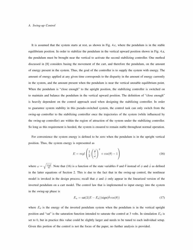
vertical for the remainder of time. Fig. 4 displays the various states of an inverted pendulum on a cart.
Fig. 4. States of the Inverted Pendulum on a Cart [8]
In this particular study, the interest lies in three distinct positions. In Fig. 4.a, the pendulum is considered
to be stabilized at an inherently unstable equilibrium point. When the pendulum is in this position, the
control is labeled as the stabilizing controller. When the system matches the position shown in Fig. 4.c, the
pendulum is considered to be in the downward position. At this point, the swing-up control will be applied
to move the pendulum to the upward position. With Figure 4.b, the pendulum is not quite stabilized nor
completely in the downward position. This particular configuration will be referred to as the transitional
period in-between the swing-up and stabilizing controllers.
A. Swing-up Control
It is assumed that the system starts at rest, as shown in Fig. 4.c, where the pendulum is in the stable
equilibrium position. In order to stabilize the pendulum in the vertical upward position shown in Fig. 4.a,
the pendulum must be brought near the vertical to activate the second stabilizing controller. One method
discussed in [8] considers basing the movement of the cart, and therefore the pendulum, on the amount
of energy present in the system. Thus, the goal of the controller is to supply the system with energy. The
amount of energy applied at any given time corresponds to the disparity in the amount of energy currently
in the system, and the amount present when the pendulum is near the vertical unstable equilibrium point.
When the pendulum is “close enough” to the upright position, the stabilizing controller is switched on
to maintain and balance the pendulum in the vertical upward position. The definition of “close enough”
is heavily dependent on the control approach used when designing the stabilizing controller. In order
to guarantee system stability in this pseudo-switched system, the control task can only switch from the
swing-up controller to the stabilizing controller once the trajectories of the system (while influenced by
the swing-up controller) are within the region of attraction of the system under the stabilizing controller.
So long as this requirement is heeded, the system is ensured to remain stable throughout normal operation.
For convenience the system energy is defined to be zero when the pendulum is in the upright vertical
position. Thus, the system energy is represented as
E = mgl
1
2
(θ
ω
)2
+ cos(θ)− 1
(16)
where ω =√
mgl4I . Note that (16) is a function of the state variables θ and θ instead of φ and φ as defined
in the latter equations of Section 2. This is due to the fact that in the swing-up control, the nonlinear
model is invoked in the design process; recall that φ and φ only appear in the linearized version of the
inverted pendulum on a cart model. The control law that is implemented to input energy into the system
in the swing-up phase is
Eu = sat(2(E − Ed))sign(θ cos(θ)) (17)
where Ed is the energy of the inverted pendulum system when the pendulum is in the vertical upright
position and “sat” is the saturation function intended to saturate the control at 3 volts. In simulation Ed is
set to 0, but in practice this value could be slightly larger and needs to be tuned to each individual setup.
Given this portion of the control is not the focus of the paper, no further analysis is provided.
B. Stabilizing Control
Once the pendulum has reached a region near the unstable equilibrium, the stabilizing controller takes
over. The primary goal of the stabilizing control is to maintain the inverted pendulum in the upright
orientation. This is achieved using three separate controllers that use either a pole-placement, H2, or H∞design approach. The particulars of each design is discussed in Section 4.
Given that the actuator, the cart motor, cannot instantaneously generated the torque necessary to move
the cart, a time delay is imposed on all three controllers of the form
1τs + 1
(18)
where τ is time constant for the transfer function in (18). Note that the value of τ is chosen relative to
the time constant of the inverted pendulum on a cart system. Moreover, the control magnitude is limited
to a value of 5 to ensure a fair comparison among all three control approaches.
C. Transition Control
Although the transition from the swing-up to the stabilizing controller should experience no instabilities,
there is no guarantee that the system will remain stable if a switch is required from the stabilizing to the
swing-up controller. If, for instance, the pendulum fails to satisfy the small angle approximations made
when constructing the linear model (i.e. the pendulum angle φ diverges too far from the vertical), the
pendulum could drop down and inadvertently reactivate the swing-up controller. To avoid exciting un-
modeled dynamics and parametric uncertainties a smoothing algorithm was utilized to ensure a smooth
transition from one control law to the next. This was done by averaging the outputs of the two controllers
near the region where the control switching occurs. However, including this algorithm in the overall control
scheme appears to provide no appreciable improvement to system performance. Thus, it has been removed
from the control architecture.
IV. STABILIZING CONTROL DESIGN
Recall the upper linear fractional transformation representation given in Section 2 in (15). This form
only includes the model uncertainty. However, when analyzing the success of the stabilizing controllers,
it is required that the external disturbances as well as the sensor noise be included in the model. The
diagram shown in Fig. 5 shows the closed-loop system in the context of all uncertainties affecting the
system performance. The variable di is the external disturbances acting on the inverted pendulum system.
These disturbances could include wind or a human interacting with the pendulum, with the caveat that
the disturbance energy is finite and belongs to a set of L2 signals, such that the magnitude is bounded
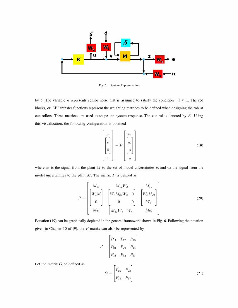
Fig. 5. System Representation
by 5. The variable n represents sensor noise that is assumed to satisfy the condition |n| ≤ 1. The red
blocks, or “W ” transfer functions represent the weighting matrices to be defined when designing the robust
controllers. These matrices are used to shape the system response. The control is denoted by K. Using
this visualization, the following configuration is obtained
zδ
e
u
z
= P
vδ
di
n
u
(19)
where zδ is the signal from the plant M to the set of model uncertainties δ, and vδ the signal from the
model uncertainties to the plant M . The matrix P is defined as
P =
M11 M12Wd M12
WeM
0
WeM22Wd 0
0 0
WeM22
Wu
M21
[M22Wd Wn
]M22
(20)
Equation (19) can be graphically depicted in the general framework shown in Fig. 6. Following the notation
given in Chapter 10 of [9], the P matrix can also be represented by
P =
P11 P12 P13
P21 P22 P23
P31 P32 P33
Let the matrix G be defined as
G =
P22 P23
P32 P33
(21)
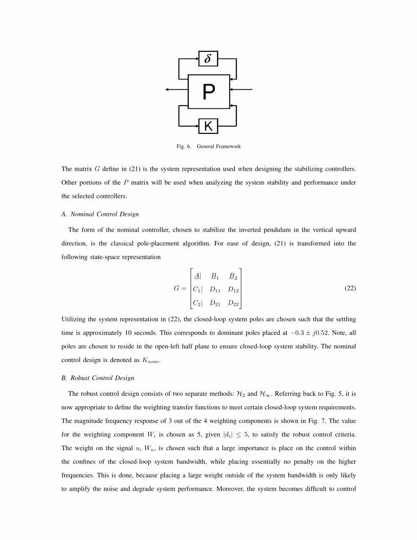
Fig. 6. General Framework
The matrix G define in (21) is the system representation used when designing the stabilizing controllers.
Other portions of the P matrix will be used when analyzing the system stability and performance under
the selected controllers.
A. Nominal Control Design
The form of the nominal controller, chosen to stabilize the inverted pendulum in the vertical upward
direction, is the classical pole-placement algorithm. For ease of design, (21) is transformed into the
following state-space representation
G =
A| B1 B2
C1| D11 D12
C2| D21 D22
(22)
Utilizing the system representation in (22), the closed-loop system poles are chosen such that the settling
time is approximately 10 seconds. This corresponds to dominant poles placed at −0.3 ± j0.52. Note, all
poles are chosen to reside in the open-left half plane to ensure closed-loop system stability. The nominal
control design is denoted as Knom.
B. Robust Control Design
The robust control design consists of two separate methods: H2 and H∞. Referring back to Fig. 5, it is
now appropriate to define the weighting transfer functions to meet certain closed-loop system requirements.
The magnitude frequency response of 3 out of the 4 weighting components is shown in Fig. 7. The value
for the weighting component Wi is chosen as 5, given |di| ≤ 5, to satisfy the robust control criteria.
The weight on the signal u, Wu, is chosen such that a large importance is place on the control within
the confines of the closed-loop system bandwidth, while placing essentially no penalty on the higher
frequencies. This is done, because placing a large weight outside of the system bandwidth is only likely
to amplify the noise and degrade system performance. Moreover, the system becomes difficult to control
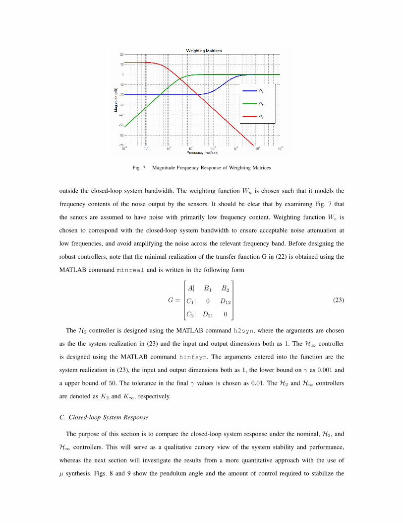
Fig. 7. Magnitude Frequency Response of Weighting Matrices
outside the closed-loop system bandwidth. The weighting function Wn is chosen such that it models the
frequency contents of the noise output by the sensors. It should be clear that by examining Fig. 7 that
the senors are assumed to have noise with primarily low frequency content. Weighting function We is
chosen to correspond with the closed-loop system bandwidth to ensure acceptable noise attenuation at
low frequencies, and avoid amplifying the noise across the relevant frequency band. Before designing the
robust controllers, note that the minimal realization of the transfer function G in (22) is obtained using the
MATLAB command minreal and is written in the following form
G =
A| B1 B2
C1| 0 D12
C2| D21 0
(23)
The H2 controller is designed using the MATLAB command h2syn, where the arguments are chosen
as the the system realization in (23) and the input and output dimensions both as 1. The H∞ controller
is designed using the MATLAB command hinfsyn. The arguments entered into the function are the
system realization in (23), the input and output dimensions both as 1, the lower bound on γ as 0.001 and
a upper bound of 50. The tolerance in the final γ values is chosen as 0.01. The H2 and H∞ controllers
are denoted as K2 and K∞, respectively.
C. Closed-loop System Response
The purpose of this section is to compare the closed-loop system response under the nominal, H2, and
H∞ controllers. This will serve as a qualitative cursory view of the system stability and performance,
whereas the next section will investigate the results from a more quantitative approach with the use of
µ synthesis. Figs. 8 and 9 show the pendulum angle and the amount of control required to stabilize the
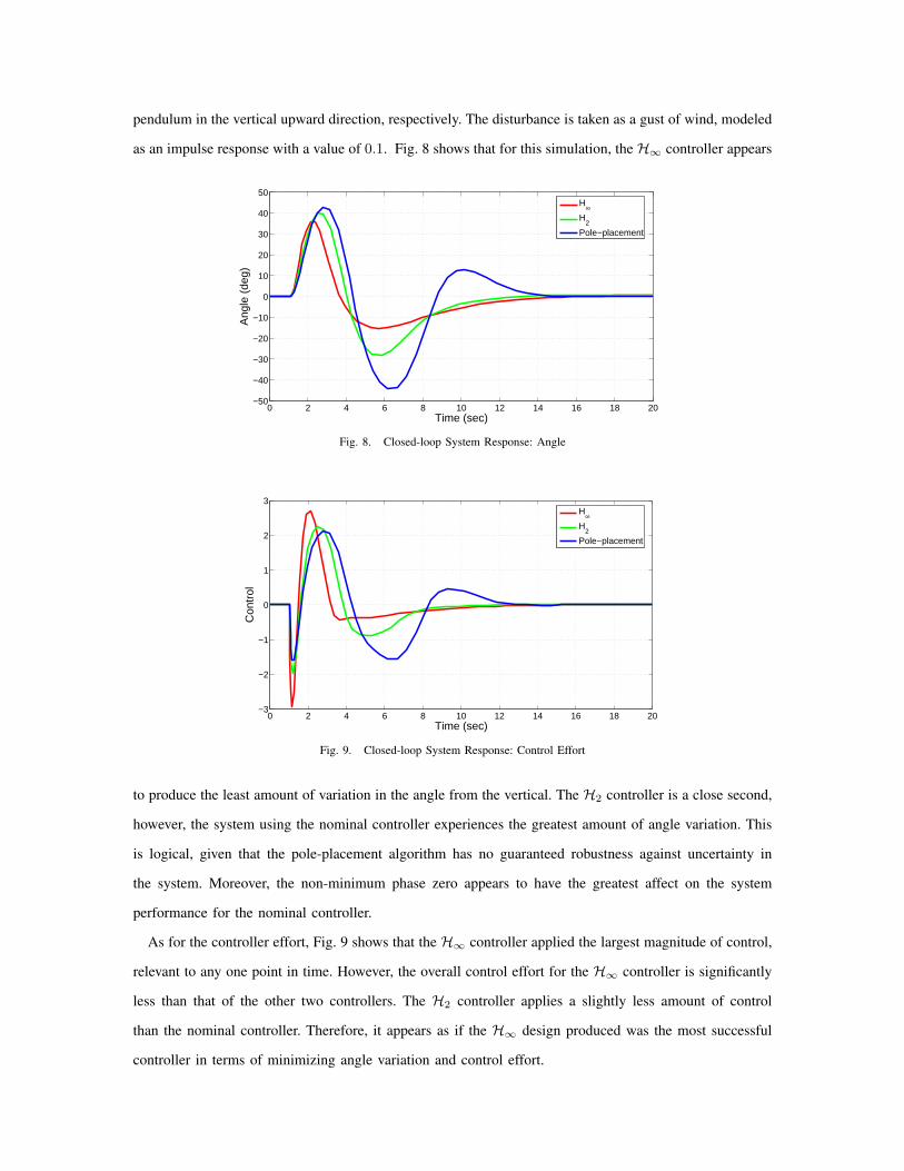
pendulum in the vertical upward direction, respectively. The disturbance is taken as a gust of wind, modeled
as an impulse response with a value of 0.1. Fig. 8 shows that for this simulation, the H∞ controller appears
0 2 4 6 8 10 12 14 16 18 20−50
−40
−30
−20
−10
0
10
20
30
40
50
Time (sec)
Ang
le (
deg)
H∞
H2
Pole−placement
Fig. 8. Closed-loop System Response: Angle
0 2 4 6 8 10 12 14 16 18 20−3
−2
−1
0
1
2
3
Time (sec)
Con
trol
H∞
H2
Pole−placement
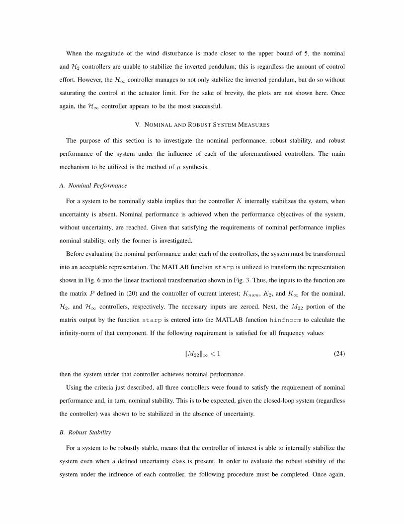
Fig. 9. Closed-loop System Response: Control Effort
to produce the least amount of variation in the angle from the vertical. The H2 controller is a close second,
however, the system using the nominal controller experiences the greatest amount of angle variation. This
is logical, given that the pole-placement algorithm has no guaranteed robustness against uncertainty in
the system. Moreover, the non-minimum phase zero appears to have the greatest affect on the system
performance for the nominal controller.
As for the controller effort, Fig. 9 shows that the H∞ controller applied the largest magnitude of control,
relevant to any one point in time. However, the overall control effort for the H∞ controller is significantly
less than that of the other two controllers. The H2 controller applies a slightly less amount of control
than the nominal controller. Therefore, it appears as if the H∞ design produced was the most successful
controller in terms of minimizing angle variation and control effort.
When the magnitude of the wind disturbance is made closer to the upper bound of 5, the nominal
and H2 controllers are unable to stabilize the inverted pendulum; this is regardless the amount of control
effort. However, the H∞ controller manages to not only stabilize the inverted pendulum, but do so without
saturating the control at the actuator limit. For the sake of brevity, the plots are not shown here. Once
again, the H∞ controller appears to be the most successful.
V. NOMINAL AND ROBUST SYSTEM MEASURES
The purpose of this section is to investigate the nominal performance, robust stability, and robust
performance of the system under the influence of each of the aforementioned controllers. The main
mechanism to be utilized is the method of µ synthesis.
A. Nominal Performance
For a system to be nominally stable implies that the controller K internally stabilizes the system, when
uncertainty is absent. Nominal performance is achieved when the performance objectives of the system,
without uncertainty, are reached. Given that satisfying the requirements of nominal performance implies
nominal stability, only the former is investigated.
Before evaluating the nominal performance under each of the controllers, the system must be transformed
into an acceptable representation. The MATLAB function starp is utilized to transform the representation
shown in Fig. 6 into the linear fractional transformation shown in Fig. 3. Thus, the inputs to the function are
the matrix P defined in (20) and the controller of current interest; Knom, K2, and K∞ for the nominal,
H2, and H∞ controllers, respectively. The necessary inputs are zeroed. Next, the M22 portion of the
matrix output by the function starp is entered into the MATLAB function hinfnorm to calculate the
infinity-norm of that component. If the following requirement is satisfied for all frequency values
‖M22‖∞ < 1 (24)
then the system under that controller achieves nominal performance.
Using the criteria just described, all three controllers were found to satisfy the requirement of nominal
performance and, in turn, nominal stability. This is to be expected, given the closed-loop system (regardless
the controller) was shown to be stabilized in the absence of uncertainty.
B. Robust Stability
For a system to be robustly stable, means that the controller of interest is able to internally stabilize the
system even when a defined uncertainty class is present. In order to evaluate the robust stability of the
system under the influence of each controller, the following procedure must be completed. Once again,
the MATLAB function starp is utilized to transform the representation shown in Fig. 6 into the linear
fractional transformation shown in Fig. 3. Thus, the inputs to the function are the matrix P defined in
(20) and the controller of current interest; Knom, K2, and K∞ for the nominal, H2, and H∞ controllers,
respectively. The necessary inputs are zeroed. Next, the M11 portion of the matrix output by the function
starp is entered into the MATLAB function mu to calculate the µ bound. The arguments entered into
this function include M11 and an array describing the perturbation block structure, denoted as “blk”. In
this case, “blk” is defined as
blk =
1 0
2 2
(25)
Given this system satisfies the necessary uncertainty dimension requirements listed in [9], the output of
this function is defined to be the bound on µ. If the following requirement is satisfied
µδ(M11) < 1, ∀ω (26)
then the system under that controller is considered to be robustly stable.
Using the criteria just described, only the two robust controllers were found to be robustly stable. This is
logical, given the nominal controller fails to take any uncertainty into account during the design phase. Note
that robust stability requires that the system be stabilized for the entire class of uncertainties define. Thus,
showing that the nominal controller is able to stabilize the system in the presence of some uncertainties
does not guarantee robust stability (as shown by the simulation provided in Section 4). The µ bounds for
the system under the nominal, H2, and H∞ controllers were 3.23, 0.54, and 0.38, respectively.
C. Robust Performance
For a system to achieve robust performance, the performance objectives must be met even when a
particular class of uncertainties is present in the system. If the system satisfies the requirements of robust
performance, that implies that it is also robustly stabilized. Similar to the previous two cases, the system
must be transformed into a robust control friendly representation. The MATLAB function starp is used
to transform the representation shown in Fig. 6 into the linear fractional transformation shown in Fig. 3.
Thus, the inputs to the function are the matrix P defined in (20) and the controller of current interest;
Knom, K2, and K∞ for the nominal, H2, and H∞ controllers, respectively. The necessary inputs are
zeroed. The matrix M , which is the output from the function starp, is then entered into the MATLAB
function mu to calculate the µ bound. The arguments entered into this function include M and an array
describing the perturbation block structure, denoted as “blk”. The “blk” array is as defined in (25). If the
following requirement is satisfied
µδ(M) < 1, ∀ω (27)
then the system is said to meet the requirements of robust performance. Only the H∞ controller was able
to satisfy the requirement given in (27). The µ bounds on both the nominal and H2 controllers exceeded
the required value of 1. However, the H∞ controller managed to produce a µ bound of approximately
0.87.
VI. CONCLUSION
This paper investigated the design and analysis of three controllers used to stabilize an inverted pendulum
on a cart. This was accomplished by decomposing each control algorithm into two separate phases: swing-up
control and stabilization control. A classical, H2, and H∞ design are each considered to stabilize a nominal
linearized model of the inverted pendulum on a cart in the upward vertical position. All three controllers
were found to meet the requirements of nominal stability and nominal performance. However, only the
robust controllers were able to achieve robust stability. Although all controllers were able to stabilize the
inverted pendulum in the vertical upward direction for some limited uncertainty, not all uncertainties chosen
within the acceptable set of finite energy bounded disturbances resulted in a stabilized system. The H∞controller was shown to achieve robust performance, whereas the other controllers allowed the system to
go unstable in the presence of large exogenous disturbances. Overall, a controller designed with uncertainty
in mind will not always be able to guarantee robust performance. This point rings particularly true when
considering that there are no guaranteed stability margins when designing a H2 controller.
REFERENCES
[1] T. McGeer, “Passive dynamic walking,” The International Journal of Robotics Research, vol. 9, no. 2, 1990.
[2] A. Kuo, J. Donelan, and A. Ruina, “Energetic consequences of walking like an inverted pendulum: Step-to-step transitions,”
Exercise and Sport Sciences Reviews, vol. 33, no. 2, 2005.
[3] R. Kram, A. Domingo, and D. Ferris, “Effect of reduced gravity on the preferred walk-run transition speed,” Journal of
Experimental Biology, vol. 200, no. 4, 1997.
[4] D. Vos and A. V. Flowtow, “Dynamics and nonlinear adaptive control of an autonomous unicycle:theory and experiment,” in
Proceedings of the 29th IEEE CDC, 1990.
[5] K. Pathak, J. Franch, and S. Agrawal, “Velocity and position control of a wheeled inverted pendulum by partial feedback
linearization,” IEEE Transactions on Robotics, vol. 21, no. 3, 2005.
[6] C. Anderson, “Learning to control an inverted pendulum using neural networks,” IEEE Control Systems Magazine, vol. 9, no. 3,
1989.
[7] S.-J. Huang and C.-L. Huang, “Control of an inverted pendulum using grey prediction model,” IEEE Transactions on Industry
Applications, vol. 36, no. 2, 2000.
[8] M. Bugeja, “Non-linear swing-up and stabilizing control of an inverted pendulum system,” in EUROCON, Ljubljana, Slovenia,
2003.

[9] K. Zhou and J. Doyle, Essentials of Robust Control. Upper Saddle River, NJ: Prentice Hall, 1998.


![Inverted Pendulum [Final]](https://static.fdocuments.in/doc/165x107/58904db31a28abcb668bcda8/inverted-pendulum-final.jpg)