10/26/2004

Robust Control 2Controllability, Observability & Transfer Functions

Harry G. KwatnyDepartment of Mechanical Engineering & MechanicsDrexel University

Outline• Reachable• Controllability• Distinguishable• Observability• Zeros• Transfer Functions• Poles• Interconnections• Stability

System

0 00

, ,n m p

tAt A(t-s)

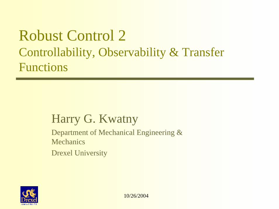
x Ax Buy Cxx R u R y R

x(t; x ,u) e x e Bu(s)ds

= +=

∈ ∈ ∈

= + ∫

Reachability

( )

1 0

0 1 0

0

A state is from if there exists a finite time 0 and a piecewise continuous control

such that . denotes the set of states reachabl

reachab

efrom .

le

Definition: nx R xt

u x(t; x ,u) x xx

∈

>

= R

Reachability: Properties

( )

( )

111 1

1 1

1 11 1

1 0 1

0 0

0

If is reachable from in some time >0, it is reachable in every time . To see this simply rescale :

Thus, we h

stt

stt

t tA(t - )A(t -s) st st

t t

tA(t- ) A(t -t) st st

t t

x x tt s

e Bu(s)ds e Bu( )d

e Be u( )d

=

=

∫ ∫

∫1

1

1 0 1 0

1 0 10

ave the replacement ( ) .______________________

Notice that is reachable from if and only if is reachable from the origin for any 0

A(t -t) stt

At

tAt A(t-s)

u s e u( )

x x x e xt

x e x e Bu(s)ds x

→

−< < ∞

= + ⇔ −∫ 00

tAt A(t-s)e x e Bu(s)ds= ∫

Some Geometry, 1

{ }

1 2

1 2

1 2

2

2 1

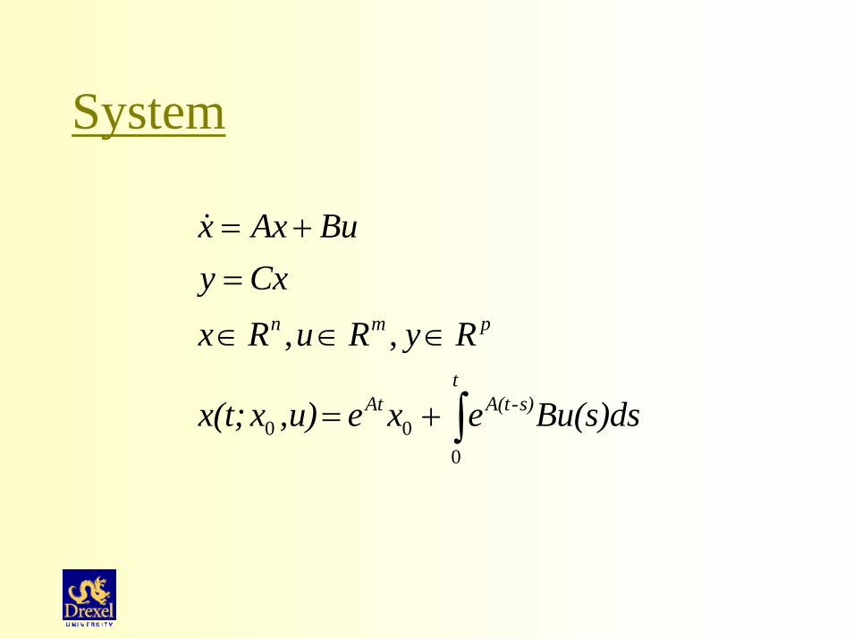
Consider two linear vector spaces , with inner products, and , ,respectively, and a mapping

:- the range or image ( Im ) of is the set of points in

,

- the null space or ker

X X

A X XA X

y X y Ax x X

→

∈ = ∈

{ }1

1

*2 1

*2 1

nel ( ker ) of is the set of points in

0

- the adjoint mapping : is defined by

, ,

A X

x X Ax

A X X

y Ax A y x

∈ =

→

=

Some Geometry, 2

( )

( )

*

** *

* *

1

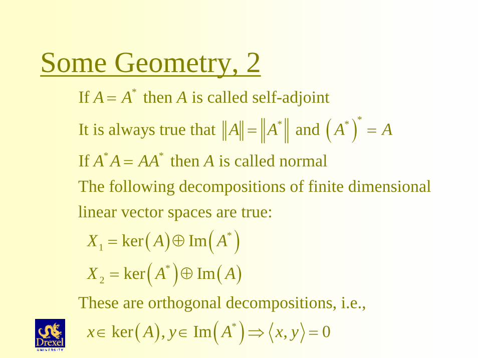
If then is called self-adjoint

It is always true that and

If then is called normalThe following decompositions of finite dimensionallinear vector spaces are true:

ker Im

A A A

A A A A

A A AA A

X A

=

= =

=

= ⊕ ( )( ) ( )

( ) ( )

*

*2

*

ker Im

These are orthogonal decompositions, i.e.,

ker , Im , 0

A

X A A

x A y A x y

= ⊕

∈ ∈ ⇒ =

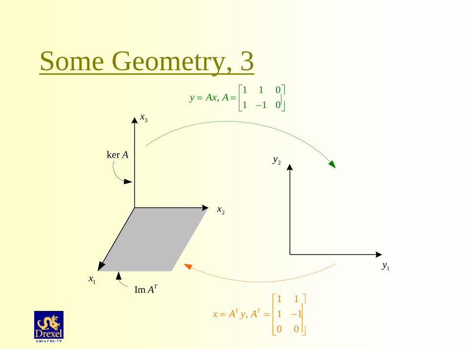
Some Geometry, 31 1 0

,1 1 0

y Ax A ⎡ ⎤= = ⎢ ⎥−⎣ ⎦

1y

2y

1x

2x

3x

1 1, 1 1

0 0

T Tx A y A⎡ ⎤⎢ ⎥= = −⎢ ⎥⎢ ⎥⎣ ⎦

Im TA

ker A

Reachability Condition

( )

( )

11

1

1

( )1 0

* *1 1 1

Let denote the linear vector space of control functions ( ), [0, ],

and the space of states . The map : is defined by

( ) (

0 Im Im note :

)

Proposit

n

t A t

x x

u t

R x t

x t e Bu d

x

τ

τ τ

τ τ−

∈ ⇔ ∈ ⇔

=

→

≅ →

∈

∈

∫

R A A

U

X A

A AA X

U

X

X

[ ]1

1 1

1

( ) ( )*

0

The set of states reachable from the origin over the time interval 0, is

Im Im

ion:

Tt A t A tT

t

e BB e dτ τ τ− −⎡ ⎤= ⎢ ⎥⎣ ⎦∫AA

Controllability

1

0

The system or the matrix pair ( , ) is said to be (completely) controllable if any state is reachable from any other state in finite time.

The system is completely contro

Definition:

Proposition:

A Bx

x

11 1

1

( ) ( )1 0

llable if an

controllability G

d only if

rank ( )where

( )

is th rammiane .

T

C

t A t A tTC

G t n

G t e BB e dτ τ τ− −

=

= ∫

Controllability Main Result

( )

1 1

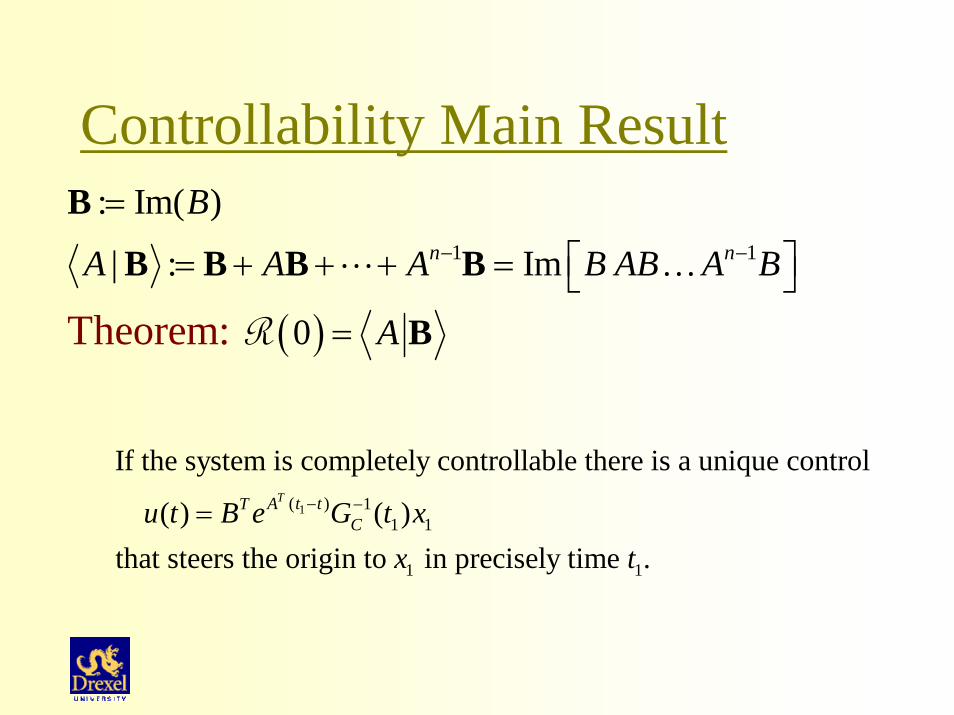
: Im( )

| : Im

0Theorem:

n n

B

A A A B AB A B

A

− −

=

⎡ ⎤= + + + = ⎣ ⎦=

B

B B B B

BR

…

1( ) 11 1

1 1

If the system is completely controllable there is a unique control

( ) ( )that steers the origin to in precisely time .

TA t tTCu t B e G t x

x t

− −=

Distinguishable

( )

1 0

1 2 0

0

A state is indistinguishable from if for every finite time and piecewise continuous control

( ), ( ; , ) ( ; , ). denotes the set of statesindistinguishable from .

:

Definition: nx R xt

u t y t x u y t x u xx

∈

= I

N ( )1

11

ker ker

(0)Theorem:

ni

in

CCA

CA

CA

−

=−

⎡ ⎤⎢ ⎥⎢ ⎥= =⎢ ⎥⎢ ⎥⎣ ⎦

=I N

∩

Observability The system or the matrix pair ( , ) is said

to be if knowledge of ( ) and ( ) on a finite time interval determines the sta

(completely) obte trajectory o

servablen

that interval.

Definition:

Theorem:

C Au t y t

1

(completely) observ

The system or the matrix pair ( , ) is if and only if (0) , i.e.

r

e

ank

abl

n

C A

CCA

n

CA −

= ∅

⎡ ⎤⎢ ⎥⎢ ⎥ =⎢ ⎥⎢ ⎥⎣ ⎦

I

Summary: Controllability/Observability1

1

1 11 12 13 14 1

2 22 24 2

3 33 34 3

4 44 4

Controllability rank

Observability rank

Kalman Decomposition, such that

0 00 00 0 0

nB AB A B n

CCA

n

CAx z

z A A A A zz A A zdz A A zdtz A z

−

−

⎡ ⎤⇔ =⎣ ⎦⎡ ⎤⎢ ⎥⎢ ⎥⇔ =⎢ ⎥⎢ ⎥⎣ ⎦

⎡ ⎤ ⎡ ⎤ ⎡⎢ ⎥ ⎢ ⎥ ⎢⎢ ⎥ ⎢ ⎥ ⎢=⎢ ⎥ ⎢ ⎥ ⎢⎢ ⎥ ⎢ ⎥ ⎢⎢ ⎥ ⎢ ⎥ ⎢⎣ ⎦ ⎣ ⎦ ⎣

[ ]11

222 4

3

4

1 2 2 4

, 0 000

, controllable , observable

zBzB

u y C Czz

z z z z

⎤ ⎡ ⎤⎡ ⎤⎥ ⎢ ⎥⎢ ⎥⎥ ⎢ ⎥⎢ ⎥+ =⎥ ⎢ ⎥⎢ ⎥⎥ ⎢ ⎥⎢ ⎥⎥ ⎢ ⎥⎣ ⎦⎦ ⎣ ⎦

Notice that the substate z2 is both controllable and

observable

Example

[ ]

[ ]

( ) [ ] [ ] ( )( )( )

( )( )

1

2 2 1, 1 0

0 4 1

1 41 4

4 210 2

1 012 4

2 12 4 4

x x u y x

B AB

ss

G s C sI A Bs s

ss s s

−

− −⎡ ⎤ ⎡ ⎤= + =⎢ ⎥ ⎢ ⎥−⎣ ⎦ ⎣ ⎦

−⎡ ⎤= = ⎢ ⎥−⎣ ⎦

+ −⎡ ⎤⎢ ⎥+ ⎡ ⎤⎣ ⎦= − = ⎢ ⎥+ + ⎣ ⎦

+= =

+ + +

C

Some MATLAB FunctionsFunctioncanon canonical stste-space realizations

ctrb controllability matrix

ctrbf controllability staircase form

gram controllability and observability gramians

obsv observability matrix

obsvf observability staircase form

ss2ss state coordinate transformation

ssbal diagonal balancing of state-space realizations

minreal returns a minimal realization

Example, Continued>> tf(sys)Transfer function:

s + 2-------------s^2 + 6 s + 8>> tf(minreal(sys))1 state removed.Transfer function:1

-----s + 4

>> A=[-2 -2;0,-4];>> B=[1;1];>> C=[1 0];>> sys=ss(A,B,C,0);>> ctrb(sys)ans =

1 -41 -4

>> gram(sys,'c')ans =

0.1250 0.12500.1250 0.1250

System Poles & Zeros

( ) [ ] 1

Two descriptions of linear time-invariant systemsstate space and transfer function.

Assumption: is a complete characterization of , , , or, equivalently, , , , is a

x Ax BuG s C sI A B D

y Cx DuG A B C D

A B C D

−= +⇔ = − +

= +

the poles of are the eigenvalues of

minimal realization of .Defining poles via state space is very easy:

.Defining zeros is more complicated. We do it via state spacein the followin .

g

GG

A

SISO System Zeros

[ ] [ ]{ }

( ) [ ]{ } ( )

[ ] [ ]

1 10

1

1 10 0

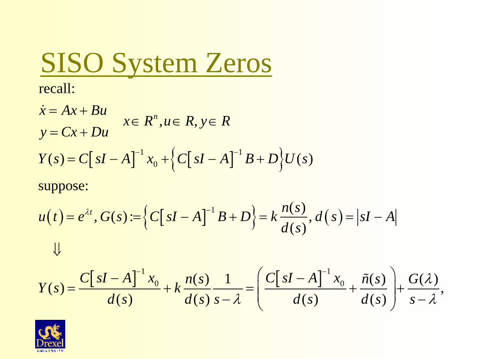
recall:

, ,

( ) ( )

suppose:( ), ( ) : ,( )

( ) 1 ( ) ( )( ) ,( ) ( ) ( ) ( )

n

t

x Ax Bux R u R y R

y Cx Du

Y s C sI A x C sI A B D U s

n su t e G s C sI A B D k d s sI Ad s

C sI A x C sI A xn s n s GY s kd s d s s d s d s s

λ

λλ λ

− −

−

− −

= +∈ ∈ ∈

= +

= − + − +

= = − + = = −

⇓

⎞⎛− −= + = + +⎟⎜⎜ ⎟− −⎝ ⎠

SISO System Zeros, Cont’d

[ ]

( ) ( ) ( ) ( )

( )

0

0

0 0

1

0

can always be chosen so that

( ) 0( ) ( )

in which case

( ) , if is a ze

In summary:if is a

ro of , then 0, 0

system zero, there exists such that

and ( )

x

C sI A x n sd s d

x

x t

s

GY s G s y t

s

u t

Y

x

λλ λ

λ

λ

− ⎞⎛ −+ ≡⎟⎜⎜ ⎟

=

=

⎝ ⎠

= =−

( ) 0

te y tλ= ⇒ ≡

MIMO System Zeros

0

0

0 0 0

0

, ,

Does there exist and such that

( ) ( ) and ( ) 0?The assumed solution must satisfy

00

n m p

m n

t t

t t t

t t

x Ax Bux R u R y R

y Cx Dug R x R

u t ge x t x e y t

x e Ax e Bge I A B xC D gCx e Dge

λ λ

λ λ λ

λ λ

λ λ

= +∈ ∈ ∈

= +

∈ ∈

= ⇒ = ≡

= + − −⎡ ⎤ ⎡ ⎤⇒ =⎢ ⎥ ⎢ ⎥−= + ⎣ ⎦ ⎣ ⎦

MIMO System Zeros, Cont’d

max

max

max

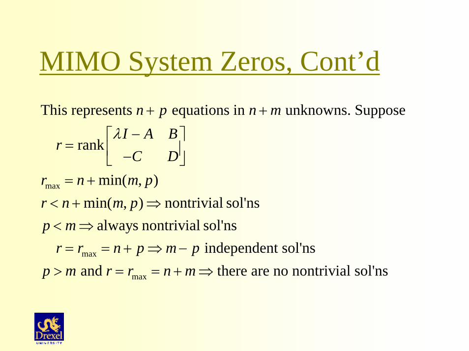
This represents equations in unknowns. Suppose

rank

min( , )min( , ) nontrivial sol'ns

always nontrivial sol'ns independent sol'ns

and ther

n p n mI A B

rC D

r n m pr n m pp m

r r n p m pp m r r n m

λ+ +

−⎡ ⎤= ⎢ ⎥−⎣ ⎦= +

< + ⇒< ⇒= = + ⇒ −

> = = + ⇒ e are no nontrivial sol'ns

Square MIMO Systems (p=m) If for typical ,

rank

Those specific values of forinva

which are called. Invariant zeros consist of

(uncontrollable mor

Nondegenerate case:

iant zerosinput decoupling zeros

I A Br n m

C Dr n m

λλ

λ

−⎡ ⎤= = +⎢ ⎥−⎣ ⎦

< +

•

[ ]des), satisfies

rank (unobservable modes), satisfies

rank

, all other invariant

output decoupling zeros

transmission zeros zeros.

I A B n

I An

C

λλ

λλ

− <

•

−⎡ ⎤<⎢ ⎥

⎣ ⎦•

Square MIMO Systems, Cont’d

( )

For typical ,

rank

0

insufficient independent controls, rank insufficient independent outputs,

degenerate case

rank

:I A B

r n mC D

G

B mC p

λλ

λ

−⎡ ⎤= < +⎢ ⎥−⎣ ⎦

≡

• <• <

Transfer Functions

( ) [ ] [ ]1 12 2 2

2 2 2

, ,

where , , are those of the Kalman decomposition -,i.e., parameters of a minimal realization.So, only the controllable and observable part of the s

n m px Ax Bux R u R y R

y Cx

G s C sI A B C sI A BA B C

− −

= +∈ ∈ ∈

=

= − = −

( )Definition: complete characterizati

ystemis characterized by its transfer function.

is called a of the system if the system is completely observable and controlla e

onbl .

G s

10/26/2004

Poles & Zeros from Transfer Functions

Numbers: Prime & CoprimeA (or integer) is a positive integer 1 that has nopositive integer divisors other than 1 and itself.

Two integers are relatively prime or if they share no pos

prime number

coprime itiveinteger factors

p >

( )

(divisors) other than 1 - i.e., their greatest common divisor is 1.

If and are integers not both zero, then thereexist integers and such thaBezout's iden

t,

If and are cop

tity

i

:

r

a bx y

GCD a b ax bya b

= +

me then there exist integers and such that1

x yax by= +

Polynomials

( )( )

11 0

11 0

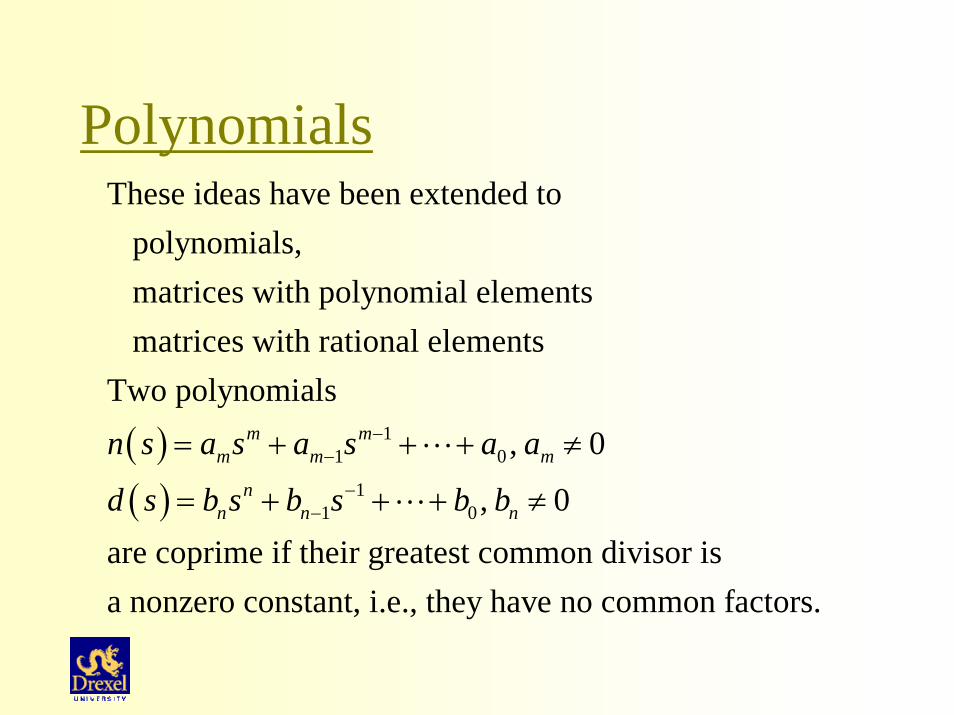
These ideas have been extended to polynomials, matrices with polynomial elements matrices with rational elementsTwo polynomials

, 0

, 0are coprime if

m mm m m

nn n n

n s a s a s a a

d s b s b s b b

−−

−−

= + + + ≠

= + + + ≠

their greatest common divisor isa nonzero constant, i.e., they have no common factors.

Example

F1 = s4 + 2s3 + s + 2 = (s + 1) (s + 2) (s2 - s + 1) F2 = s5 + s4 + 2s3 + 3s2 + 3s + 2 = (s + 1) (s2 - s + 2) (s2 + s + 1)

gcd(F1,F2) = (s + 1)

Bezout relation: (5/24s3 + 1/12s2 + 1/4s + 5/24) F1 + (-5/24s2 - 7/24s + 7/24) F2

= s + 1

Polynomial Matrices

( )( )

( )( ) ( ) ( ) ( ) ( ) ( )( ) ( )

11 0 , ,

11 0

,right common d

Two matrix polynomials

,

have a if

,

, are if the only right common

divisors are unim

ivisor

right coprime

A B

m mm m p q p q

i inn n

q q

N s A s A s AA R B R

D s B s B s B

R s R

N s N s R s D s D s R s

N s D s

−−

−−

= + + +∈ ∈

= + + +

∈

= =

( )odular, i.e., det 0.Similary, left coprimeness can be defined for polynomialmatrices with the same number of rows.

R s c= ≠

Poles( )

( )( ) ( ) ( ) ( ) ( )1 1

Suppose the transfer matrix is a complete characterization of,

can always be factored into

where , and , are coprime pairs of polynomial matrices. l l r r

l l r r

q m G sx Ax Bu y Cx Du

G s

G s D s N s N s D sD N D N N

− −

×

= + = +

= =

[ ] ( )

[ ] ( )

1 2 1 2

, and , are called numerator, denominator matrices, respectively.

det det (Definition: Pol

) det , are constants. are the roots of:

det 0, or det

Theore

( ) 0, or det

m

0e

:s

r l

r r

l r

l r

ND D

sI A D s D s

sI A D s D s

α α α α− = =

− = = =

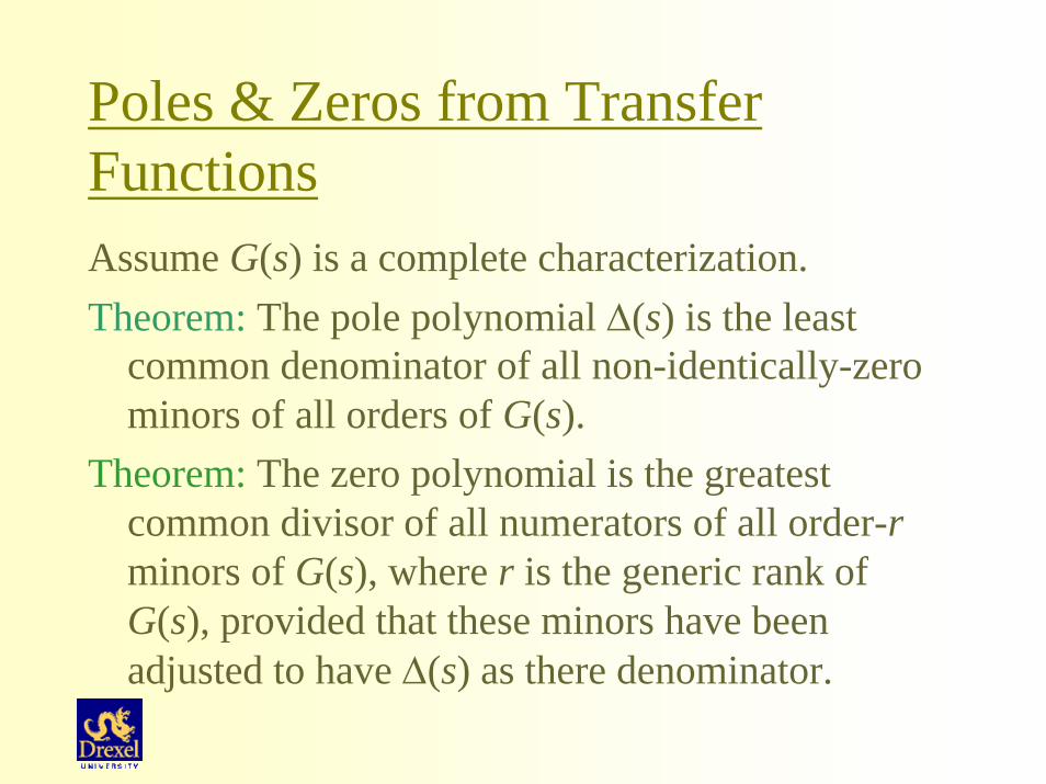
Poles & Zeros from Transfer FunctionsAssume G(s) is a complete characterization.Theorem: The pole polynomial ∆(s) is the least

common denominator of all non-identically-zero minors of all orders of G(s).

Theorem: The zero polynomial is the greatest common divisor of all numerators of all order-rminors of G(s), where r is the generic rank of G(s), provided that these minors have been adjusted to have ∆(s) as there denominator.

Recall a minor of a matrix is the determinant of a matrix obtained by deleting rows and columns.Example

( ) ( )

( )

Consider the transfer function:1 41

4.5 2 12To determine poles we need all minors of all orders.The 4 minors of order 1 are

1 4 4.5 1, , ,22 2 2 2

rank =2.

The single minor of order 2 i

sG s

ss

s ss s s s

G s

−⎡ ⎤= ⎢ ⎥−+ ⎣ ⎦

− −+ + + +

( ) ( )( )( )

4s det 22

pole polynomial: 2

zero polynomial: 4

sG ss

s s

z s s

φ

−=

+

= +

= −

10/26/2004

Multivariable Interconnections & Feedback Loops

Well-Posed Loops: Example( )G s

( )

( ) ( ) ( )

[ ]( ) ( )

1

1

11

1 21 1

1 11

Let , be proper rational transfer matrices.Then

is proper and rational iff is nonsin

T

gula

he

r

m:

.

ore

cl

cl

sG ss

s ss s

G s G s I G ss

G H

G G I HG

I H G

−

−

⎡ ⎤−⎢ ⎥= ⎢ ⎥

− −⎢ ⎥⎢ ⎥+ +⎣ ⎦

− + − −⎡ ⎤= + =⎡ ⎤ ⎢ ⎥⎣ ⎦ −⎣ ⎦

= +

+ ∞ ∞

Poles of Closed Loops( )G s

( )H s

[ ]

[ ]

1

It might be anticipated that the poles of arethe roots of det . Not True!!

cl

cl

G G I HGG

I HG

−= +

+

( ) ( )

( ) [ ]

21 1 ,

211

21 1 , det 1

211

obviously, has poles at 1.

cl

s ss sG s H s I

ss s

s sG s I HGss

s

−⎡ ⎤⎢ ⎥− += = ⇒⎢ ⎥

−⎢ ⎥⎢ ⎥+⎣ ⎦

−⎡ ⎤⎢ ⎥+ += + ≡ −⎢ ⎥

−⎢ ⎥−⎢ ⎥−⎣ ⎦= ±

Poles, Cont’d

( ) ( )

( ) ( ) ( ) ( ) ( )

( )( )( ) ( )

( )( ) ( )

If , are proper, reational matrices and

det 0, then the poles of are the

roots of the polyn

Example:1 1

0.5 1.5 0.

omial

d

Theor

e

50.5 1

0.5 1.5 .5

e :

0

t

m

cl

G H

G H

I H G G

s s s

s s sG s

ss s s

I H s G s

+ ∞ ∞ ≠⎡ ⎤⎣ ⎦

∆ = ∆ ∆ +⎡ ⎤⎣

⎡ ⎤⎢ − + −⎢=⎢ +

− +⎣

⎦

⎢ −⎢ ⎦

2, H I⎥⎥ =⎥⎥⎥

Poles: Example Cont’d( )

( ) ( )( ) ( ) ( ) ( )( )

( )( )

( ) ( )

( )( )1

0.5det0.5

1.5 0.5 , 1 1.5 0.5

100.5

1 11.5 1.5

0 1.5 1 01.5 0.5

0.5 0.5 0 1

G H

cl

sI G ss

s s s s s s s

sG s

s s

ss s

s s

−

++ =⎡ ⎤⎣ ⎦ −

∆ = + − ∆ = ⇒ ∆ = + +

⎡ ⎤⎢ ⎥−⎢ ⎥=⎢ ⎥⎢ ⎥+ +⎢ ⎥⎣ ⎦

+ ⎛ ⎞⎡ ⎤ ⎡ ⎤= + +⎜ ⎟⎢ ⎥ ⎢ ⎥+ +⎣ ⎦ ⎣ ⎦⎝ ⎠

System Interconnections1 2

1 1

1 2

1 2

Systems , are complete characterizations, with

, 1,2 coprime fractions. parallel connection

controllable , left coprime

observable , right coprime series connecti

i li li ri ri

r r

l l

G G

G D N N D i

D D

D D

− −= = =

•

⇔

⇔

•

( ) ( )

2 1 1 2 1 2 2 1

1 2 1 2 2 1 2 1

2 1

1 2

oncontrollable , , or , or , are left coprimeobservable , , or , or , right coprime

det 0. Then

controllable controllableobservable

r r l r l l l r

l r l r r r l r

D N D D N D N N

D N D D N D N N

I G G

G GG

⇔

⇔

• + ∞ ∞ ≠⎡ ⎤⎣ ⎦⇔⇔ 2 1 observableG

1G

2G

1G

2G

2G1G

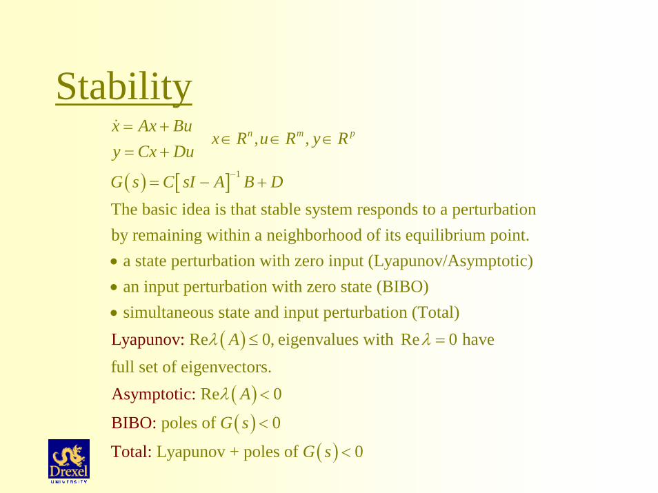
Stability

( ) [ ] 1

, ,

The basic idea is that stable system responds to a perturbationby remaining within a neighborhood of its equilibrium point. a state perturbation with zero i

n m px Ax Bux R u R y R

y Cx Du

G s C sI A B D−

= +∈ ∈ ∈

= +

= − +

•

( )

nput (Lyapunov/Asymptotic) an input perturbation with zero state (BIBO) simultaneous state and input perturbation (Total)

Re 0, eigenvalues with Re 0 havefull set of eigenvLyapunov:

Asympecto

tors.

t

Aλ λ

••

≤ =

( )( )

( )

ic:

BIBO:

To

Re 0

poles of 0

Lyapunov + poles ofal: t 0

A

G s

G s

λ <

<

<