ROBUST ANTENNA ARRAY BEAMFORMING UNDER ...2.2. Conventional Adaptive Beamforming Using Signal...

Progress In Electromagnetics Research B, Vol. 35, 307–328, 2011

ROBUST ANTENNA ARRAY BEAMFORMING UNDERCYCLE FREQUENCY MISMATCH

J.-H. Lee*

Department of Electrical Engineering, Graduate Institute of Commu-nication Engineering, and Graduate Institute of Biomedical Electronicsand Bioinformatics, National Taiwan University, No. 1, Sec. 4, Roo-sevelt Rd., Taipei 10617, Taiwan

Abstract—Many algorithms exploiting the signal cyclostationarityhave been shown to be effective in performing antenna arraybeamforming. However, these algorithms can not provide a uniqueweight vector for simultaneously extracting multiple signals of interest(SOIs) with distinct cycle frequencies (DCFs). They also sufferfrom severe performance degradation in the presence of a cyclefrequency error (CFE). To simultaneously accommodate multiple SOIswith DCFs and alleviate the effects of cycle leakage due to finitedata samples, we propose a cyclic sample matrix inversion (C-SMI)beamformer. To make the C-SMI beamformer robust against CFE,we present a novel objective function which is optimized by using asteepest-descent based algorithm to find the appropriate estimates ofthe true DCFs. The simulation results show the effectiveness of therobust C-SMI beamformer.

1. INTRODUCTION

For conventional adaptive array beamforming, we require the prioriinformation of either the impinging direction or the waveform of thedesired signal to adapt the weights [l, 2]. A steered-beam beamformeris taught by the actual direction vector of the desired signal andforced to make a constant response in the desired signal direction.Hence, its performance is very sensitive to the accuracy of the steeringvector. However, the true direction vector of the desired signal maynot be exactly known in some applications, e.g., the application in landmobile-cellular radio systems. Hence, we often encounter the problem

Received 22 August 2011, Accepted 22 October 2011, Scheduled 1 November 2011* Corresponding author: Ju-Hong Lee ([email protected]).

308 Lee

of mismatch between the real direction vector of the desired signal andthe steering vector. The effectiveness of a steered-beam beamformercan be destroyed even if a small mismatch arises [2, 17–20].

In contrast, adaptive beamforming utilizing signal cyclostation-arity has been developed due to two main reasons. Based on thecyclostationary property, we can solve the problem of blind adaptivebeamforming, i.e., an adaptive beamformer can automatically preservethe desired signal while cancelling noise and interference without anypriori information about the desired signal direction [3]. Moreover,cyclostationarity is a statistical property possessed by most of practi-cal man-made communication signals [4, 5]. Another cyclic adaptivebeamforming (CAB) algorithm and two more complicated CAB-basedalgorithms, namely, the constrained CAB (C-CAB) and the robustCAB (R-CAB), were also proposed in [6] to enhance the performanceof the CAB algorithm. However, these three algorithms are eigenvalueproblems and work for extracting either one signal of interest (SOI)or multiple SOIs with the same cycle frequency. For multiple SOIshaving distinct cycle frequencies (DCFs), they treat each SOI as asingle signal. It has been shown in [6] that the least-squares spectralself-coherence restoral (LS-SCORE) and C-CAB algorithms have thesame asymptotical maximum output signal-to-interference plus noiseratio (SINR) performance as the number of data snapshots approachesinfinite. Among these blind beamforming techniques, the LS-SCOREapproach [3] has been extensively considered [7] because of its sim-plicity in avoiding the computationally expensive eigen-decompositionor singular-value decomposition (SVD) in implementation. The prioriinformation that the original LS-SCORE approach requires to work isonly the cycle frequency of the SOI. Hence, its performance is sensi-tive to the accuracy of the presumed cycle frequency. However, theactual cycle frequency of the SOI may not be known exactly in someapplications due, for example, to the phenomenon of Doppler shift.The research work in [8, 9] has presented an analytical formula thatdemonstrates the behavior of the performance degradation due to cyclefrequency error (CFE) for the LS-SCORE approach. The output SINRof an adaptive blind beamformer using the LS-SCORE approach dete-riorates like a sinc function as the number of data snapshots increases.Robust approaches based on the LS-SCORE algorithm were then pre-sented in [8, 9] for estimating the true cycle frequency. Recently, threerobust algorithms based on the CAB algorithm of [6] were developedin [10] to deal with CFE. The subspace constrained CAB (SC-CAB)algorithm simply projects the CAB weight vector onto the signal-plus-interference subspace to alleviate the steering vector error due to CFE.The robust SC-CAB algorithm is a combination of the SC-CAB algo-

Progress In Electromagnetics Research B, Vol. 35, 2011 309

rithm and the robust idea based on optimization of worst-case perfor-mance [11]. A convex second-order cone optimization problem withan optimal value of the diagonal loading factor must be solved underthe uncertainty of the SC-CAB weight vector. The structured steer-ing vector (SSV) algorithm estimates the direction vector of the SOIfrom the SC-CAB weight vector. Then it finds the SSV weight vectorby minimizing the array output power with a distortionless constrainttowards the estimated SOI’s direction vector. These three robust algo-rithms work for extracting either only one SOI or multiple SOIs withthe same cycle frequency. Besides these three CAB-based robust al-gorithms are still eigenvalue problems, they cannot provide a uniqueweight vector for simultaneously receiving multiple SOIs with DCFs.

In this paper, we consider adaptive blind beamforming undermultiple SOIs with DCFs. To simultaneously accommodate multipleSOIs with DCFs and alleviate the effects of cycle leakage due to finitedata samples, a cyclic sample matrix inversion (C-SMI) beamformerwhich is developed based on the conventional SMI beamformer withthe exploitation of signal cyclostationarity and diagonal loading. Tomake the C-SMI beamformer robust against CFE, we present a novelobjective function to formulate an optimization problem. The trueDCFs can be estimated by solving the optimization problem througha steepest-descent based iterative algorithm with the exploitation ofsignal cyclostationarity. The C-SMI beamformer with the iterativealgorithm effectively provides a weight vector for simultaneouslyextracting multiple SOIs with DCFs against CFE.

This paper is organized as follows. In Section 2, we brieflydescribe the original LS-SCORE algorithm of [3]. The C-SMIbeamformer for adaptive blind beamforming under multiple SOIs withDCFs is presented in Section 3. We present the theoretical workfor alleviating the performance degradation caused by the CFE inSection 4. The convergence analysis of the proposed approach ispresented in Section 5. Several computer simulation examples forconfirming the effectiveness of the proposed approach are provided inSection 6. Finally, we conclude the paper in Section 7.

2. CONVENTIONAL ADAPTIVE BEAMFORMINGUSING CYCLOSTATIONARITY

2.1. Signal Cyclostationarity

Cyclostationarity is a statistical property possessed by most ofpractical man-made communication signals. A signal r (t) withcyclostationarity has the property that its cyclic correlation function(CCF) and cyclic conjugate correlation function (CCCF) given by the

310 Lee

following infinite time averages

Rrr(α, τ) =⟨r(t)r∗(t− τ)e−j2παt

⟩∞

and Rrr∗(α, τ) =⟨r(t)r(t− τ)e−j2παt

⟩∞ (1)

respectively, are not equal to zero at some time delay τ andcycle frequency α, where the superscript “*” denotes the complexconjugate. It has been shown in [9] that many modulated signalsexhibit cyclostationarity with cycle frequency equal to twice the carrierfrequency or multiples of the baud rate or combinations of these. Forthe data vector x (t) received by an antenna array with N isotropicsensor elements, the associated cyclic correlation matrix (CCM) andcyclic conjugate correlation matrix (CCCM) are given by

Rxx(α, τ) =⟨x(t)xH(t− τ)e−j2παt

⟩∞

and Rxx∗(α, τ) =⟨x(t)xT (t− τ)e−j2παt

⟩∞ , (2)

respectively, where the superscripts “H” and “T” denote the conjugatetranspose and the complex conjugate, respectively.

2.2. Conventional Adaptive Beamforming Using SignalCyclostationarity

Consider an adaptive beamformer using an M -element antenna arrayexcited by a signal of interest (SOI), J interferers, and spatially whitenoise. The received data vector x (t) is given by

x(t) = s(t)a(θd) +J∑

j=1

sj(t)a(θj) + n(t) = s(t)a(θd) + i(t), (3)

where s(t) and sj (t) denotes the waveforms of the SOI and the jthinterferer, a (θd) and a (θj) the direction vectors of the SOI withdirection angle θd and the jth interferer with direction angle θj , andn(t) the noise vector, respectively. The array output is given byy(t) = wHx(t), where w denotes the weight vector of the beamformer.Assume that s(t) is cyclostationary and has a cycle frequency α, buti (t) is not cyclostationary at α and is temporally uncorrelated withs(t). According to the original LS-SCORE algorithm of [3], a costfunction is defined as follows:

G(w; c) =⟨|y(t)− r(t)|2

⟩T

, (4)

where the reference signal r (t) is given by

r(t) = cHx∗(t− τ)ej2παt (5)


and < · >T denotes the average over the time interval [0,T ]. c is afixed control vector. The optimal weight vector wls minimizing (4) isgiven by [3]

wls = R−1xx rxr(α), (6)

where Rxx =⟨x(t)xH(t)

⟩T and rxr(α) = 〈x(t)r∗(t)〉T are the sample

correlation matrix of x (t) and the sample cross-correlation vector ofx (t) and r (t) computed over [0,T ], respectively. For any control vectorc as long as cHa(θd) 6= 0, it is shown in [3] that (6) converges to thesolution of conventional adaptive beamforming based on the maximumoutput SINR criterion as T approaches infinite.

3. ADAPTIVE BLIND BEAMFORMING WITHMULTIPLE CYCLE FREQUENCIES

Assume that there are D uncorrected SOIs with direction angles θd

and DCFs αd, d = 1, 2, . . ., D and J interferers. The received datavector x (t) becomes

x(t)=D∑

d=1

sd(t)a(θd)+D+J∑

j=D+1

sj(t)a(θj)+n(t)=D∑

d=1

sd(t)a(θd)+i(t). (7)

To accommodate the D SOIs, we use the following reference signal

r(α1, α2, . . . , αD; t) =D∑

d=1

ej2παdtcHx∗(t− τ). (8)

Let the interferers and noise do not have the cycle fre-quencies equal to αd, d = 1, 2, . . ., D. It is shownin Appendix A that the corresponding rxr(α1, α2, . . . , αD) =〈x(t)r∗(α1, α2, . . . , αD; t)〉T approaches rxr (α1, α2, . . ., αD) =D∑

d=1

traceRxx(αd, 0)ρsds∗d(αd, 0) / Mρsdsd(αd, 0)a(θd) as T ap-

proaches infinity, where ρsdsd(αd, 0) and ρsds∗d (αd, 0) denote the cyclic

correlation coefficient (CCC) and cyclic conjugate correlation coeffi-cient (CCCC) of sd (t) computed at τ = 0, respectively. As a result,rxr (α1, α2, . . . , αD) can be used as a weight vector to retrieve the DSOIs. However, the effects of cycle leakage due to finite data sam-ples as shown by [8, 9] will be significant if we directly set the beam-former’s weight vector equal to rxr(α1, α2, . . . , αD). To alleviate theeffects of cycle leakage, we propose an approach based on the results

312 Lee

of Appendix A. First, the CCC and CCCC of sd (t) are given as fol-lows [12, 13] :

ρsdsd(αd, τ) =

Rsdsd(αd, τ)

rsdsd

and ρsds∗d(αd, τ) =Rsds∗d(αd, τ)

rsdsd

, (9)

respectively, where rsdsddenotes the average power of sd (t). For a

given cyclostationary signal sd (t), its ρsdsd(αd, τ)and ρsds∗d(αd, τ) can

be computed in advance. Using (9) and (A4), we obtain the averagepower of sd (t) as follows:

rsdsd=

trace Rxx(αd, τ)Mρsdsd

(αd, τ). (10)

Moreover, the CCCF Rsds∗d (αd, τ) of sd (t) can be obtained from (9)and (10) as follows:

Rsds∗d(αd, τ) = ρsds∗d(αd, τ)× trace Rxx(αd, τ)Mρsdsd

(αd, τ). (11)

Therefore, the correlation matrix Rss due to the D uncorrected SOIscan be expressed as

Rss = E

(D∑

d=1

sd(t) a(θd)

)(D∑

d=1

sd(t) a(θd)

)H

=D∑

d=1

rsdsda(θd)a(θd)H . (12)

Based on (A6) of Appendix A, we can obtain a (θd) as follows:

a(θd) = ρsdsd(αd, 0)Mrxr(αd)

/traceRxx(αd,0)ρsds∗d(αd, 0). (13)

Therefore, we note from (13) that rxr(αd) can be viewed as a consistentestimate of a (θd). In case of finite data samples, we can set theestimate a (θd) of a (θd) equal to the normalized version of rxr(αd), i.e.,a(θd) = rxr(αd)/(rxr(1)

√M), where rxr(1) denotes the first element

of rxr(αd). Substituting (13) into (12) yields

Rss =D∑

d=1

trace Rxx(αd, 0)Mρsdsd

(αd, 0)ρsdsd

(αd, 0)Mrxr(αd)

/traceRxx(αd, 0)ρsds∗d(αd, 0) × ρsdsd(αd, 0)Mrxr(αd)

/traceRxx(αd, 0)ρsds∗d(αd, 0)H . (14)


The correlation matrix Rii due to the interference plus noise can beobtained as follows:

Rii = Rxx −Rss

= Ex(t)x(t)H −D∑

d=1

trace Rxx(αd, 0)Mρsdsd

(αd, 0)ρsdsd

(αd, 0)Mrxr(αd)

/traceRxx(αd,0)ρsds∗d(αd, 0) × ρsdsd(αd, 0)Mrxr(αd)

/traceRxx(αd,0)ρsds∗d(αd, 0)H . (15)

The above procedure proposed for obtaining Rii does not need to solveany eigenvalue problem. In contrast, the R-CAB algorithm [6] basedon the C-CAB algorithm does need to solve an eigenvalue problem forcomputing Rii.

To compute an efficient weight vector wnew for simultaneouslyreceiving multiple cyclostationary signals with DCFs, we combine thesample matrix inversion (SMI) beamformer [1] with the exploitation ofsignal cyclostationarity and the diagonal loading (DL) [14] as follows:

wnew = (Rii + κI)−1rxr(α1, α2, . . . , αD), (16)

where Rii denotes the sample version of Rii computed by takingthe data samples over the time interval [0,T ], I the M × Midentity matrix, and wnew the sample version of wnew = (Rii +κI)−1rxr(α1, α2, . . . , αD). We term the beamformer with the weightvector of (16) as the cyclic SMI (C-SMI) beamformer. Since the noiseeigenvalues associated with Rii show random variation due to thefinite sample data, the noise eigenvectors affect the SMI beamformer’sresponse in a manner determined by the variation of the correspondingrandom eigenvalues. As a result, a conventional SMI beamformersuffers from the addition of randomly weighted noise eigenvectors andhence higher sidelobe level in its adaptive beam pattern. Adding theloading factor κ in (16) is to add the loading level to all the eigenvaluesassociated with Rii and hence produces a bias in the noise eigenvaluesto reduce their random variation. To enhance the performance of theC-SMI beamformer, the loading factor κ is usually chosen according tothe power level of the SOIs. According to our simulation experience, itis appropriate to set κ to a large value so that κI dominates the term(Rii +κI) when the D SOIs are strong. In contrast, κ is set to a smallvalue so that Rii dominates when the D SOIs are weak. Hence, anappropriate choice for κ is given by

κ = traceRss

, (17)

314 Lee

where Rss denotes the sample version of Rss computed over the timeinterval [0,T ]. Recently, an ad-hoc way developed for conventionalstandard Capon beamformer to determine the loading factor level waspresented in [16].

To make a comparison between the proposed C-SMI beamformerand the LS-SCORE beamformer for simultaneously receiving multiplecyclostationary signals with DCFs, we modify the original LS-SCOREweight vector of (6) by replacing the rxr(α) with rxr(α1, α2, . . . , αD),i.e., the weight vector is set to wls = R−1

xx rxr(α1, α2, . . . , αD).

4. ROBUST BLIND BEAMFORMING AGAINST CFE

Here, we present a robust approach for performing blind beamformingagainst CFE. First, consider the concept for conventional linearlyconstrained minimum variance (LCMV) beamforming with main-beam constraint [1]. The optimum weight vector wLCMV is obtainedby minimizing the array output power subject to the steered-beamconstraint as follows:

Minimize wHLCMVRxxwLCMV Subject to wLCMVa(θd) = 1, (18)

where θd is the SOI’s direction angle. It is easy to show that theminimum value of wH

LCMVRxxwLCMV corresponding to the optimumsolution of wLCMV is equal to the inverse of a (θd)HR−1

xxa (θd). Usingthis result and (A6) of Appendix A, we propose an objective functionQ (α1, α2, . . . , αD) for the considered problem as follows:

Q(α1, α2, . . . , αD) = rxr(α1, α2, . . . , αD)HR−1xx rxr(α1, α2, . . . , αD),(19)

where α1, α2, . . ., and αD represent the estimates of α1, α2, . . . ,and αD, respectively. Clearly, this objective function reaches itsmaximum when the estimates α1, α2, . . . , αD are equal to the actualα1, α2, . . . , αD, respectively. To find the appropriate estimates forthe DCFs α1, α2, . . . , αD, we formulate the following optimizationproblem:

Maximizeα1,α2,....,αD

rxr(α1, α2, . . . , αD)HR−1xx rxr(α1, α2, . . . , αD), (20)

To solve (20), we adapt the method of steepest descent by taking thederivatives of the objective function Q (α1, α2, . . . , αD) with respect to


α1, α2, . . . , αD. The derivatives are given by

∇αd

Q(α1, α2, . . . , αD) =∂Q(α1, α2, . . . , αD)

∂αd

=∂rxr(α1, α2, . . . , αD)HR−1

xx rxr(α1, α2, . . . , αD)∂αd

=∂rxr(α1, α2, . . . , αD)H

∂αdR−1

xx rxr(α1, α2, . . . , αD)

+rxr(α1, α2, . . . , αD)HR−1xx

∂rxr(α1, α2, . . . , αD)∂αd

= 2× real

rxr(α1, α2, . . . , αD)HR−1

xx

∂rxr(α1, α2, . . . , αD)∂αd

= 2× realrxr(α1, α2, . . . , αD)HR−1

xx rxud(αd)

, (21)

for d = 1, 2, . . . , D, whererxud

(αd) = ∂ 〈x(t)r∗(α1, α2, . . . , αD; t)〉T /∂αd

=⟨x(t)xT (t)ce−j2παdt(−j2πt)

⟩T

. (22)

Since the objective function Q (α1, α2, . . . , αD) reaches the maximumat α1, α2, . . . , αD, it should be approximately a concave function inan appropriate neighborhood of α1, α2, . . . , αD. Accordingly, theupdated value of the estimate for the cycle frequency αd at the timeinstant ti+1 can be computed by using the following recursive formula:

αd(ti+1) = αd(ti) + νd(ti) ∇αd

Q(α1, α2, . . . , αD)|α1 = α1(ti), α2 = α2(ti), . . . , αD = αD(ti), (23)

for d = 1, 2, . . . ,D, where νd (ti) is a positive real-valued parameterreferred to as the step-size parameter. Examining the derivatives givenby (21), we set the step-size parameter equal to

νd(ti) =1∥∥∥

⟨x(t)xT (t)e−j2παd(ti)t(−j2πt)

⟩ti

∥∥∥pd

(24)

for d = 1, 2, . . . , D, to ensure the convergence of the steepest-descentbased algorithm used by (23), where ||B|| denotes the maximumsingular value of the matrix B. As shown in the next section, pd is apositive real value which must be appropriately determined to ensurethe convergence. The updated weight vector at the time instant ti+1

is obtained by substituting (23) into (16) and given by

wnew(ti+1)=(Rii(ti+1)+κI

)−1rxr

(α1(ti+1), α2(ti+1), . . . , αD(ti+1)

), (25)

316 Lee

where Rii(ti+1) denotes the sample version of Rii computed in thetime interval [0, ti+1] with ti+1 = (i + 1)Ts and the sampling period =Ts.

5. CONVERGENCE OF THE PROPOSED APPROACH

From (19), we can obtain the following expression after some algebraicmanipulations

Q(α1(ti), α2(ti), . . . , αD(ti)) = rxr(α1(ti), α2(ti), . . . , αD(ti))HR−1xx(ti)

rxr(α1(ti),α2(ti), . . . , αD(ti))=1i2

i−1∑

l=0

i−1∑

k=0

D∑

u=1

D∑

v=1

cHx∗(l)xT (k)c

×xH(l)R−1

xx(ti)x(k)

ej2π(lαu−kαv)Ts , (26)

where we add the time index ti to indicate that the objective function iscomputed at the time instant ti. From (7), the term xH(l)R−1

xx(ti)x(k)can be approximated as follows:

xH(l)R−1xx(ti)x(k) ≈

D∑

d=1

s∗d(l)sd(k)a(θd)HR−1

xx(ti)a(θd)

+D+J∑

j=D+1

s∗j (l)sj(k)a(θj)HR−1

xx(ti)a(θj)

+ noise-related terms. (27)

(27) is obtained due to a(θd)HR−1xx(ti)a(θj)≈ 0 and a(θj)HR−1

xx(ti)a(θj)≈ 0as the number i of data snapshots approaches infinity, j, j = D +1, 2, . . . , D + J and j 6= j. The term cHx∗(l)xT (k)c can be expressedas follows:

cHx∗(l)xT (k)c = cH

D∑

d=1

sd(l) a(θd) +J∑

j=1

sj(l) a(θj) + n(l)

∗

D∑

d=1

sd(k) a(θd) +D+J∑

j=D+1

sj(k) a(θj) + n(k)

T

c

=D∑

d=1

s∗d(l)sd(k)cH a∗(θd)aT (θd)c

+

D+J∑

j=D+1

s∗j (l)sj(k)

cH a∗(θj)aT (θj)c

+ cH n∗(l)nT (k)c+ cross terms. (28)

We have from (27) and (28) that


cHx∗(l)xT (k)c

xH(l)R−1

xx(ti)x(k)

≈D∑

d=1

s∗d(l)s∗d(l)sd(k)sd(k)

a(θd)HR−1

xx(ti)a(θd)

cH a∗(θd)aT (θd)c

+D+J∑

j=D+1

s∗j (l)s∗j (l)sj(k)sj(k)

a(θj)HR−1

xx(ti)a(θj)


+the cross terms including noise and interference. (29)

As the number i of data snapshots approaches infinity, wesubstitute (29) into (26) and perform some necessary algebraicmanipulations to obtain


rxr(α1(ti), α2(ti), . . . , αD(ti)) ≈D∑

d=0

D∑

u=1

D∑

v=1

1i2

i−1∑

l=0

i−1∑

k=0

sd(l)sd(l)

e−j2πlαuTs

∗×

sd(k)sd(k)e−j2πkαvTs

×

a(θd)HR−1

xx(ti)a(θd)

×cHa∗(θd)aT(θd)c

+

D+J∑

j=D+1

D∑

u=1

D∑

v=1

1i2

i−1∑

l=0

i−1∑

k=0

sj(l)sj(l)e−j2πlαuTs

∗

×sj(k)sj(k)e−j2πkαvTs

×

a(θj)HR−1

xx(ti)a(θj)×

cHa∗(θj)aT (θj)c

=D∑

d=1

[D∑

u=1

D∑

v=1

Rsds∗d(αu, 0)∗Rsds∗d(αv, 0)

×

a(θd)HR−1

xx(ti)a(θd)

×cHa∗(θd)aT(θd)c

]+

D+J∑

j=D+1

[D∑

u=1

D∑

v=1

Rsjs∗j (αu, 0)∗Rsjs∗j (αv, 0)

×a(θj)HR−1

xx(ti)a(θj)×


]. (30)

The cross terms disappear in (30) because of the stationarity ofn (t) and the assumed uncorrelation among sd (t), sj(t), and n(t).From (30), we can rewrite (21) as

318 Lee

∇αd

Q(α1(ti), α2(ti), . . . , αD(ti)) =∂Q(α1(ti),α2(ti), . . . , αD(ti))

∂αd

≈D∑

d=1

[[∂

D∑

u=1

D∑

v=1

Rsdsd∗(αu, 0)∗Rsdsd∗(αv, 0)

/∂αd

]

×a(θd)HR−1

xx(ti)a(θd)×


]

+J∑

j=1

[[∂

D∑

u=1

D∑

v=1


/∂αd

]

×a(θj)HR−1

xx(ti)a(θj)×


]. (31)

Consider BPSK signals. We set

sd(t) = Adej(παdt+Φsd

(t)) and sj(t) = Ajej(παjt+Φsj (t)), (32)

where Ad and Aj are the constant amplitudes, and Φsd(t) and Φsj (t)

are the random phases equal to ±(π/2) for d = 1, 2, . . . , D andj = D + 1, . . . , D + J , respectively. Accordingly, we have

Rsds∗d(αu, 0) = −A2d sinc((αu − αd)T )

and Rsjs∗j (αu, 0) = −A2j sinc((αu − αj)T ). (33)

Based on (32), it can be shown that

∂

D∑

u=1

D∑

v=1


/∂αd

= A4d

D∑

v=1

∂sinc((αd − αd)T )∂αd

sinc((αv − αd)T )+

D∑

u=1

∂sinc((αd − αd)T )∂αd

sinc((αu − αd)T )


and

∂

D∑

u=1

D∑

v=1


/∂αd

= A4j

D∑

v=1

∂sinc((αd − αj)T )∂αd

sinc((αv − αj)T )+

D∑

u=1

∂sinc((αd − αj)T )∂αd

sinc((αu − αj)T )

. (34)

Let αd = αd + ∆αd and αd − αq = ∆αdq. It is appropriate toconsider the case where the interval T = iTs is so large that all theterms sinc (∆αdqT ) are negligible for all d 6= q. Therefore, we canapproximate (34) as follows:

∂

D∑

u=1

D∑

v=1


/∂αd|αd=αd(i)

= 2A4d

∂sinc(∆αdiTs)∂∆αd

|∆αd=∆αd(i)sinc(∆αd(i)iTs)

=2π∆αd(i)iTs cos(π∆αd(i)iTs)−sin(π∆αd(i)iTs)

π∆α2d(i)iTs

A4dsinc(∆αd(i)iTs)

and ∂

D∑

u=1

D∑

v=1

Rsjs∗j(αu, 0)∗Rsjs∗j(αv, 0)

/∂αd≈0 (35)

if we can make sure that the following condition given by

|∆αd(i)iTs| ≤ 12

(36)

is satisfied, where ∆αd(i) = αd(i)−αd denotes the estimation error ofαd at the time instant T = iTs. As a result, (31) becomes

∇αd

Q(α1(ti),α2(ti), . . . , αD(ti)) =∂Q(α1(ti),α2(ti), . . . , αD(ti))

∂αd

≈D∑

d=1

[[2π∆αd(i)iTs cos(π∆αd(i)iTs)− sin(π∆αd(i)iTs)

π∆α2d(i)iTs

A4d

sinc(∆αd(i)iTs)

]×

a(θd)HR−1

xx(ti)a(θd)×

cHa∗(θd)aT(θd)c

](37)

320 Lee

and the term⟨x(t)xT (t)e−j2παd(ti)t(−j2πt)

⟩ti

of (24) becomes


⟩ti≈

D∑

d=1

A2de−jπ∆αd(i)iTs

π∆α2d(i)iTs

×

sin(π∆αd(i)iTs)− π∆αd(i)iTs cos(π∆αd(i)iTs)+ jπ∆αd(i)iTs sin(π∆αd(i)iTs)

a(θd)a(θd)T . (38)

We note that the maximum singular value of (38) is approximatelyequal to

M2A2d

π∆α2d(i)iTs

∣∣∣∣sin(π∆αd(i)iTs)− π∆αd(i)iTs cos(π∆αd(i)iTs)+ jπ∆αd(i)iTs sin(π∆αd(i)iTs)

∣∣∣∣ . (39)

Therefore, the step-size parameter of (24) is approximately given by

νd(ti) =1∥∥∥


⟩ti

∥∥∥pd

≈

M2A2d

π∆α2d(i)iTs

∣∣∣∣sin(π∆αd(i)iTs)−π∆αd(i)iTscos(π∆αd(i)iTs)+jπ∆αd(i)iTssin(π∆αd(i)iTs)

∣∣∣∣−pd

. (40)

Next, we consider the objective function shown by (30). Aftersubstituting (33) into (30), we have


rxr(α1(ti), α2(ti), . . . , αD(ti)) =D∑

d=1

[D∑

u=1

D∑

v=1

A4dsinc((αu − αd)T )

sinc((αv − αd)T )

×

a(θd)HR−1

xx(ti)a(θd)×


]

+D+J∑

j=D+1

[D∑

u=1

D∑

v=1

A4j sinc((αu − αj)T )sinc((αv − αj)T )

×a(θj)HR−1

xx(ti)a(θj)×


]. (41)

Again, we can approximate (41) as follows:


rxr(α1(ti), α2(ti), . . . , αD(ti)) ≈D∑

d=1

A4

dsinc2(∆αdT )×

a(θd)H

R−1xx(ti)a(θd)

×

cHa∗(θd)aT (θd)c

(42)


when the interval T = iTs is so large that all the terms sinc (∆αdqT )are negligible for all d 6= q.

From the update formula of (23), we have that∆αd(ti+1) = ∆αd(ti) + νd(ti) ∇

αd

Q(α1, α2, . . . , αD)|α1 = α1(ti), α2 = α2(ti), . . . , αD = αD(ti) (43)

and∆αd(i + 1)(i + 1)Ts ≈

∆αd(i) + 2M−2pdA4−2pds

a(θd)HR−1

xx (ti)a(θd)

×cHa(θd)∗a(θd)Tc

× sinc(∆αd(i)iTs)

×π∆αd(i)iTs cos(π∆αd(i)iTs)−sin(π∆αd(i)iTs)(π∆α2

d(i)iTs

)1−pd

× |sin(π∆αd(i)iTs)− π∆αd(i)iTs cos(π∆αd(i)iTs)

+jπ∆αd(i)iTs sin(π∆αd(i)iTs)|−pd

(i + 1)Ts. (44)

Setting ∆αd(i)(iTs) to the extreme value 1/2 and performingsome necessary algebraic manipulations, we have the followingapproximation

∆αd(i + 1)(i + 1)Ts ≈ 12

+12i− Ω× i + 1

ipd−1, (45)

where Ω =

24−2pdπpd−2M−2pdA4−2pds a(θd)HR−1

xx (ti)a(θd)×cHa(θd)∗a(θd)TcT 2−pd

s

×

(1 + π2

4

)−pd/2. Ω is always non-negative and approximately indepen-

dent of i by neglecting the finite sample effect. Under the condition|∆αd(i)iTs| ≤ 1

2 of (36), we have that

−1 ≤ 12(i− 1)

− Ωi

(i− 1)pd−1≤ 0. (46)

Equation (46) leads to that

(i− 1)pd−2

2i≤ Ω ≤ (2i− 1)(i− 1)pd−2

2i. (47)

Based on (36), we have to ensure that |∆αd(i + 1)(i + 1)Ts| ≤ 12.

From (47), we obtain12i− (2i− 1)(i + 1)

2ipd(i− 1)2−pd≤ 1

2i− Ω

i + 1ipd−1

≤ 12i− i + 1

2ipd(i− 1)2−pd. (48)

322 Lee

Hence, setting 1 ≤ pd ≤ 2 leads to

12i− i + 1

2ipd(i− 1)2−pd=

12i

[1−

(i + 1

i

)pd−1 (i + 1i− 1

)2−pd]≤ 0

and 12i −

(2i−1)(i+1)

2ipd (i−1)2−pd> −1 if pd = 2 and < −1 if pd = 1. Therefore,

there exists some pd between 1 and 2 such that |∆αd(i+1)(i+1)Ts| ≤ 12

for d = 1, 2, . . . , D. Following the similar procedure, we can provethat the conclusion is also valid for substituting the other extremevalue −1/2 for ∆αd(i)(iTs) into (44) and performing some necessaryalgebraic manipulations.

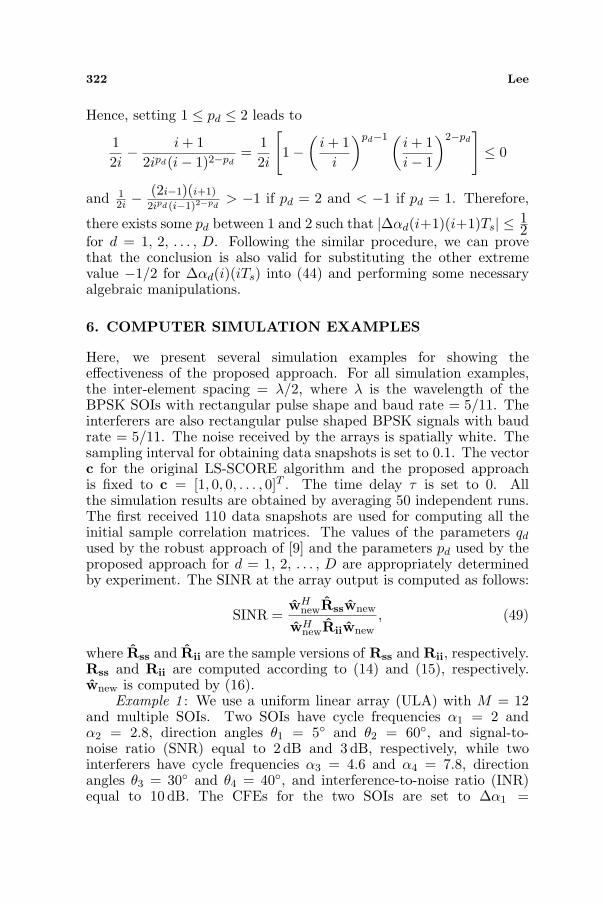
6. COMPUTER SIMULATION EXAMPLES

Here, we present several simulation examples for showing theeffectiveness of the proposed approach. For all simulation examples,the inter-element spacing = λ/2, where λ is the wavelength of theBPSK SOIs with rectangular pulse shape and baud rate = 5/11. Theinterferers are also rectangular pulse shaped BPSK signals with baudrate = 5/11. The noise received by the arrays is spatially white. Thesampling interval for obtaining data snapshots is set to 0.1. The vectorc for the original LS-SCORE algorithm and the proposed approachis fixed to c = [1, 0, 0, . . . , 0]T . The time delay τ is set to 0. Allthe simulation results are obtained by averaging 50 independent runs.The first received 110 data snapshots are used for computing all theinitial sample correlation matrices. The values of the parameters qd

used by the robust approach of [9] and the parameters pd used by theproposed approach for d = 1, 2, . . . , D are appropriately determinedby experiment. The SINR at the array output is computed as follows:

SINR =wH

newRsswnew

wHnewRiiwnew

, (49)

where Rss and Rii are the sample versions of Rss and Rii, respectively.Rss and Rii are computed according to (14) and (15), respectively.wnew is computed by (16).

Example 1 : We use a uniform linear array (ULA) with M = 12and multiple SOIs. Two SOIs have cycle frequencies α1 = 2 andα2 = 2.8, direction angles θ1 = 5 and θ2 = 60, and signal-to-noise ratio (SNR) equal to 2 dB and 3 dB, respectively, while twointerferers have cycle frequencies α3 = 4.6 and α4 = 7.8, directionangles θ3 = 30 and θ4 = 40, and interference-to-noise ratio (INR)equal to 10 dB. The CFEs for the two SOIs are set to ∆α1 =


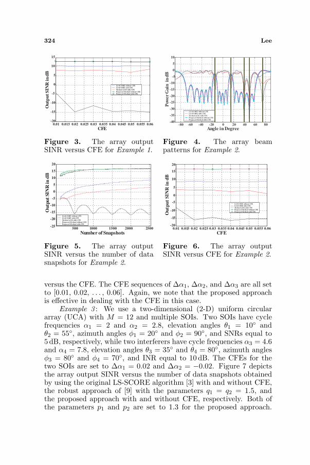
0.02 and ∆α2 = −0.02. Figure 1 plots the array beam patternswith 2530 data snapshots obtained by using the original LS-SCOREalgorithm [3] with and without CFE, the robust approach of [9] withthe parameters q1 = q2 = 1.5, and the proposed approach with andwithout CFE, respectively. The parameters p1 and p2 are set to 1.32and 1.3, respectively for the proposed approach. The array outputSINRs are −12.776, 10.532, 7.949, 12.736, and 12.949 dB, respectively.Figure 2 depicts the array output SINR versus the number of datasnapshots. Figure 3 demonstrates the array output SINR versusthe CFE. The CFE sequences of ∆α1 and ∆α2 are [0.01, 0.02, . . . ,0.06] and [−0.01, −0.02, . . . , −0.06], respectively. We note that theproposed approach is effective in dealing with the CFE problem andprovides the performance better than that of using the original LS-SCORE algorithm without CFE.

Example 2 : We use a ULA with M = 18 and multiple SOIs. ThreeSOIs have cycle frequencies α1 = 2, α2 = 2.8, and α3 = 9.4, directionangles θ1 = −15, θ2 = 15, and θ3 = 75, and SNR equal to 5 dB,while two interferers have cycle frequencies α3 = 4.6 and α4 = 7.8,direction angles θ3 = 40 and θ4 = 50, and INR equal to 15 dB. TheCFEs for the SOIs are set to ∆α1 = ∆α2 = ∆α3 = 0.02. Figure 4plots the array beam patterns with 2530 data snapshots obtained byusing the original LS-SCORE algorithm [3] with and without CFE,the robust approach of [9] with the parameters q1 = q2 = q3 = 1.8,and the proposed approach with and without CFE, respectively. Theparameters p1, p2, and p3 are all set to 1.32 for the proposed approach.The array output SINRs are −16.236, 8.625, 3.141, 16.957, and17.057 dB, respectively. Figure 5 depicts the array output SINR versusthe number of data snapshots. Figure 6 shows the array output SINR

-80 -60 -40 -20 0 20 40 60 80-40

-35

-30

-25

-20

-15

-10

-5

0

5

10

Angle in Degree

Po

wer G

ain

in

dB

LS-SCORE without CFE

LS-SCORE with CFE

Method of [9] with CFE

Proposed Method without CFE

Proposed Method with CFE

Figure 1. The array beampatterns for Example 1.

500 1000 1500 2000 2500-20

-15

-10

-5

0

5

10

15

Number of Snapshots

Ou

tpu

t S

INR

in

dB


LS-SCORE with CFE




Figure 2. The array outputSINR versus the number of datasnapshots for Example 1.

324 Lee

0.01 0.015 0.02 0.025 0.03 0.035 0.04 0.045 0.05 0.055 0.06-20

-15

-10

-5

0

5

10

15

CFE

Ou

tpu

t S

INR

in

dB


LS-SCORE with CFE




Figure 3. The array outputSINR versus CFE for Example 1.

-80 -60 -40 -20 0 20 40 60 80-40

-35

-30

-25

-20

-15

-10

-5

0

5

10

Angle in Degree

Pow

er G

ain

in

dB


LS-SCORE with CFE




Figure 4. The array beampatterns for Example 2.

500 1000 1500 2000 2500-25

-20

-15

-10

-5

0

5

10

15

20

Number of Snapshots

Ou

tpu

t SIN

R in d

B


LS-SCORE with CFE





0.01 0.015 0.02 0.025 0.03 0.035 0.04 0.045 0.05 0.055 0.06-20

-15

-10

-5

0

5

10

15

20

CFE

Ou

tpu

t S

INR

in

dB


LS-SCORE with CFE





versus the CFE. The CFE sequences of ∆α1, ∆α2, and ∆α3 are all setto [0.01, 0.02, . . . , 0.06]. Again, we note that the proposed approachis effective in dealing with the CFE in this case.

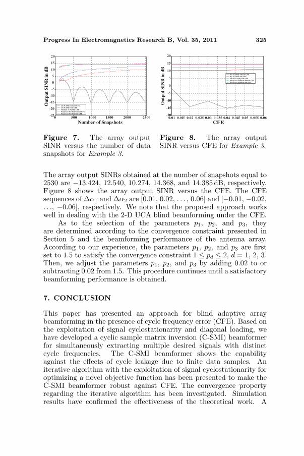
Example 3 : We use a two-dimensional (2-D) uniform circulararray (UCA) with M = 12 and multiple SOIs. Two SOIs have cyclefrequencies α1 = 2 and α2 = 2.8, elevation angles θ1 = 10 andθ2 = 55, azimuth angles φ1 = 20 and φ2 = 90, and SNRs equal to5 dB, respectively, while two interferers have cycle frequencies α3 = 4.6and α4 = 7.8, elevation angles θ3 = 35 and θ4 = 80, azimuth anglesφ3 = 80 and φ4 = 70, and INR equal to 10 dB. The CFEs for thetwo SOIs are set to ∆α1 = 0.02 and ∆α2 = −0.02. Figure 7 depictsthe array output SINR versus the number of data snapshots obtainedby using the original LS-SCORE algorithm [3] with and without CFE,the robust approach of [9] with the parameters q1 = q2 = 1.5, andthe proposed approach with and without CFE, respectively. Both ofthe parameters p1 and p2 are set to 1.3 for the proposed approach.


0 500 1000 1500 2000 2500-25

-20

-15

-10

-5

0

5

10

15

20

Number of Snapshots

Ou

tpu

t S

INR

in

dB


LS-SCORE with CFE





0.01 0.015 0.02 0.025 0.03 0.035 0.04 0.045 0.05 0.055 0.06-20

-15

-10

-5

0

5

10

15

20

CFE

Ou

tpu

t S

INR

in

dB


LS-SCORE with CFE

Mehtod of [9] with CFE




The array output SINRs obtained at the number of snapshots equal to2530 are −13.424, 12.540, 10.274, 14.368, and 14.385 dB, respectively.Figure 8 shows the array output SINR versus the CFE. The CFEsequences of ∆α1 and ∆α2 are [0.01, 0.02, . . . , 0.06] and [−0.01, −0.02,. . ., −0.06], respectively. We note that the proposed approach workswell in dealing with the 2-D UCA blind beamforming under the CFE.

As to the selection of the parameters p1, p2, and p3, theyare determined according to the convergence constraint presented inSection 5 and the beamforming performance of the antenna array.According to our experience, the parameters p1, p2, and p3 are firstset to 1.5 to satisfy the convergence constraint 1 ≤ pd ≤ 2, d = 1, 2, 3.Then, we adjust the parameters p1, p2, and p3 by adding 0.02 to orsubtracting 0.02 from 1.5. This procedure continues until a satisfactorybeamforming performance is obtained.

7. CONCLUSION

This paper has presented an approach for blind adaptive arraybeamforming in the presence of cycle frequency error (CFE). Based onthe exploitation of signal cyclostationarity and diagonal loading, wehave developed a cyclic sample matrix inversion (C-SMI) beamformerfor simultaneously extracting multiple desired signals with distinctcycle frequencies. The C-SMI beamformer shows the capabilityagainst the effects of cycle leakage due to finite data samples. Aniterative algorithm with the exploitation of signal cyclostationarity foroptimizing a novel objective function has been presented to make theC-SMI beamformer robust against CFE. The convergence propertyregarding the iterative algorithm has been investigated. Simulationresults have confirmed the effectiveness of the theoretical work. A

326 Lee

further research work on the extension of the proposed approach todeal with random cycle frequency mismatch as discussed in [15] iscurrently under investigation.

APPENDIX A.

From (7) and (8), the cross-correlation vector of x (t) and r(t) iscomputed over [0,T ] as follows:

rxr(α1, α2, . . . , αD) =⟨x(t)r∗(t)

⟩T

=

⟨(D∑

d=1sd(t)a(θd) + i(t)

)(D∑

d=1

ej2παdtcHx∗(t− τ)

)∗⟩

T

. (A1)

As T approaches infinity, it follows from the proof of [7] that (A1) canbe approximated by

limT→∞

rxr(α1, α2, . . . , αD) = limT→∞

〈x(t)r∗(t)〉T = rxr(α1, α2, . . . , αD)

= 〈x(t)r∗(t)〉∞ =D∑

d=1

kdRsds∗d(αd, τ)a(θd) =D∑

d=1

Sda(θd), (A2)

where kd = aT (θd)ce−jπαdτ , Rsds∗d(αd, τ) =⟨sd(t)sd(t− τ)e−j2παdt

⟩∞,

and Sd = kdRsds∗d(αd, τ). From (A2), we note that the parameter Sd,for d = 1, 2, . . . , D, can be obtained as follows. From (2), the CCMRxx(αd, τ) is given byRxx(αd, τ)=

⟨x(t)xH(t−τ)e−j2παdt

⟩∞=Rsdsd

(αd, τ)a(θd)aH(θd). (A3)Hence, we havetraceRxx(αd, τ) = Rsdsd

(αd, τ)aH(θd)a(θd) = MRsdsd(αd, τ). (A4)

Accordingly, the CCF Rsdsd(αd, τ) of sd (t) can be obtained from

(A4) as follows: Rsdsd(αd, τ) = traceRxx(αd, τ)/M . Next, setting

the M × 1 control vector to c = [1 0 0 . . . 0]T and τ = 0, we havekd = aT (θd)ce−jπτ = 1 since the first array sensor is the reference. Asa result, Sd is given bySd =Rsds∗d(αd, 0)=ρsds∗d(αd, 0)traceRxx(αd, 0)/Mρsdsd

(αd, 0),(A5)for d = 1, 2, . . . , D. It follows that (A2) can be rewritten asrxr(α1, α2, . . . , αD) = lim

T→∞rxr(α1, α2, . . . , αD) = lim

T→∞〈x(t)r∗(t)〉T

=D∑

d=1

Sda(θd) =D∑

d=1

ρsds∗d(αd, 0)trace

Rxx(αd,0)a(θd)/Mρsdsd(αd, 0). (A6)


ACKNOWLEDGMENT

This work was supported by the National Science Council of TAIWANunder Grants NSC96-2221-E002-086 and NSC97-2221-E002-174-MY3.The author would like to thank Mr. H.-H. Chan for his helpin preparing MATLAB programs to obtain the simulation resultspresented in the paper.

REFERENCES

1. Monzingo, R. A. and T. W. Miller, Introduction to AdaptiveArrays, John Wiley, New York, 1980.

2. Compton, Jr., R. T., Adaptive Antennas, Concepts, andPerformance, Prentice Hall, Englewood Cliffs, NJ, 1989.

3. Agee, B. G., S. V. Schell, and W. A. Gardner, “Spectral self-coherence restoral: A new approach to blind adaptive signalextraction using antenna arrays,” Proc. IEEE, Vol. 78, No. 4, 753-767, Apr. 1990.

4. Gardner, W. A., “Spectral correlation of modulated signals: PartI — Analog modulation,” IEEE Trans. on Commun., Vol. 35,No. 6, 584-594, Jun. 1987.

5. Gardner, W., W. Brown, and C.-K. Chen, “Spectral correlation ofmodulated signals: Part II — Digital modulation,” IEEE Trans.on Commun., Vol. 35, No. 6, 595–601, Jun. 1987.

6. Wu, Q. and K. M. Wong, “Blind adaptive beamforming forcyclostationary signals,” IEEE Trans. on Signal Processing,Vol. 44, No. 11, 2757–2767, Nov. 1996.

7. Yu S.-J. and J.-H. Lee, “Adaptive array beamforming forcyclostationary signals,” IEEE Trans. on Antennas and Propagat.,Vol. 44, No. 7, 943–953, Jul. 1996.

8. Lee, J.-H. and Y.-T. Lee, “Robust adaptive array beamforming forcyclostationary signals under cycle frequency error,” IEEE Trans.on Antennas and Propagat., Vol. 47, No. 2, 233–241, Feb. 1999.

9. Lee, J.-H., Y.-T. Lee, and W.-H. Shih, “Efficient robust adaptivebeamforming for cyclostationary signals,” IEEE Trans. on SignalProcessing, Vol. 48, No. 7, 1893–1901, Jul. 2000.

10. Tang, H., K. M. Wong, A. B. Gershman, and S. Vorobyov, “Blindadaptive beamforming for cyclostationary signals with robustnessagainst cycle frequency mismatch,” Proc. of IEEE Sensor Arrayand Multichannel Signal Processing Workshop, 18–22, Rosslyn,VA, USA, Aug. 2002.

328 Lee

11. Vorobyov, S. A., A. B. Gershman, and Z.-Q. Luo, “Robustadaptive beamforming using worst-case performance optimization:A solution to the signal mismatch problem,” IEEE Trans. onSignal Processing, Vol. 51, No. 2, 313–324, Feb. 2003.

12. Gardner, W. A., Statistical Spectral Analysis: A NonprobabilisticTheory, Prentice Hall, Englewood Cliffs, NJ, 1988.

13. Gardner, W. A., “Exploitation of spectral redundancy incyclostationary signals,” IEEE Signal Processing Mag., 14–36,Apr. 1991.

14. Wang, Z. and P. Stoica, “On robust Capon beamforming anddiagonal loading,” IEEE Trans. on Signal Processing, Vol. 51,No. 7, 1702–1715, Jul. 2003.

15. Lee, Y.-T. and J.-H. Lee, “Robust adaptive array beamformingwith random error in cycle frequency,” IEE Proc. Radar, Sonarand Navigation, Vol. 148, 193–199, Aug. 2001.

16. Lin, D., J. Li, and P. Stoica, “Fully automatic computation ofdiagonal loading levels for robust adaptive beamforming,” IEEETrans. on Aerospace and Electronic Systems, Vol. 46, No. 1, 449–458, Jan. 2010.

17. Li, Y., Y.-J. Gu, Z.-G. Shi, and K. S. Chen, “Robust adaptivebeamforming based on particle filter with noise unknown,”Progress In Electromagnetics Research, Vol. 90, 151–169, 2009.

18. Mallipeddi, R., J. P. Lie, P. N. Suganthan, S. G. Razul, andC. M. S. See, “Near optimal robust adaptive beamforming ap-proach based on evolutionary algorithm,” Progress In Electromag-netics Research B, Vol. 29, 157–174, 2011.

19. Mallipeddi, R., J. P. Lie, S. G. Razul, P. N. Suganthan, andC. M. S. See, “Robust adaptive beamforming based on covariancematrix reconstruction for look direction mismatch,” Progress InElectromagnetics Research Letters, Vol. 25, 37–46, 2011.

20. Lee, J.-H., G.-W. Jung, and W.-C. Tsai, “Antenna arraybeamforming in the presence of spatial information uncertainties,”Progress In Electromagnetics Research B, Vol. 31, 139-156, 2011.

ROBUST ANTENNA ARRAY BEAMFORMING UNDER ...2.2. Conventional Adaptive Beamforming Using Signal...

Documents

Transcript of ROBUST ANTENNA ARRAY BEAMFORMING UNDER ...2.2. Conventional Adaptive Beamforming Using Signal...