Robust and Adaptive Multigrid Methods: comparing ...
25
NUMERICAL LINEAR ALGEBRA WITH APPLICATIONS Numer. Linear Algebra Appl. 0000; 00:1–25 Published online in Wiley InterScience (www.interscience.wiley.com). DOI: 10.1002/nla Robust and Adaptive Multigrid Methods: comparing structured and algebraic approaches S.P. MacLachlan 1, * , J.D. Moulton 2 , and T.P. Chartier 3 1 Department of Mathematics, Tufts University, 503 Boston Avenue, Medford, MA 02155, USA. 2 Applied Mathematics and Plasma Physics, MS B284, Los Alamos National Laboratory, Los Alamos, NM 87545, USA 3 Department of Mathematics, Davidson College, Box 6908, Davidson, NC 28035, USA. SUMMARY Although there have been significant advances in robust algebraic multigrid methods in recent years, numerical studies and emerging hardware architectures continue to favor structured-grid approaches. Specifically, implementations of logically structured robust variational multigrid algorithms, such as the Black Box Multigrid (BoxMG) solver, have been shown to be 10 times faster than AMG for three-dimensional heterogeneous diffusion problems on structured grids [1]. BoxMG offers important features such as operator-induced interpolation for robustness, while taking advantage of direct data access and bounded complexity in the Galerkin coarse-grid operator. Moreover, since BoxMG uses a variational framework, it can be used to explore advances of modern adaptive AMG approaches in a structured setting. In this paper, we show how to extend the adaptive multigrid methodology to the BoxMG setting. This extension not only retains the favorable properties of the adaptive framework, but also sheds light on the relationship between BoxMG and AMG. In particular, we show how classical BoxMG can be viewed as a special case of classical AMG, and how this viewpoint leads to a richer family of adaptive BoxMG approaches. We present numerical results that explore this family of adaptive methods and compare its robustness and efficiency to the classical BoxMG solver. Copyright c 0000 John Wiley & Sons, Ltd. Received . . . KEY WORDS: Multigrid, Adaptive Multigrid, Algebraic Multigrid 1. INTRODUCTION While multigrid methods have been actively studied since the seminal work of Brandt in the 1970’s [2,3], the field remains one of active research, with recent advances in robustness from the adaptive multigrid framework [4–7] and application to a wide variety of new problems [8–12]. Additionally, the challenges of evolving computer architectures have driven research into numerical methods that are naturally suited to GPUs and other accelerated architectures [13–15]. In this paper, we consider the implementation of the adaptive multigrid methodology * Correspondence to: S. P. MacLachlan, Department of Mathematics, Tufts University, 503 Boston Avenue, Medford, MA 02155, USA. [email protected] Contract/grant sponsor: The work of SPM was partially supported by the National Science Foundation, under grant DMS-0811022. The work of JDM was funded by the Department of Energy at Los Alamos National Laboratory under contracts DE-AC52-06NA25396 and the DOE Office of Science Advanced Computing Research (ASCR) program in Applied Mathematical Sciences. The work of TPC was partially supported by a research fellowship from the Alfred P. Sloan Foundation and the Department of Energy, under grant DE-FG02-04ER25590. Copyright c 0000 John Wiley & Sons, Ltd. Prepared using nlaauth.cls [Version: 2010/05/13 v2.00]
Transcript of Robust and Adaptive Multigrid Methods: comparing ...
NUMERICAL LINEAR ALGEBRA WITH APPLICATIONSNumer. Linear Algebra Appl. 0000; 00:1–25Published online in Wiley InterScience (www.interscience.wiley.com). DOI: 10.1002/nla
Robust and Adaptive Multigrid Methods: comparing structuredand algebraic approaches
S.P. MacLachlan1,∗, J.D. Moulton2, and T.P. Chartier3
1 Department of Mathematics, Tufts University, 503 Boston Avenue, Medford, MA 02155, USA.2 Applied Mathematics and Plasma Physics, MS B284, Los Alamos National Laboratory,Los Alamos, NM 87545, USA3 Department of Mathematics, Davidson College, Box 6908, Davidson, NC 28035, USA.
SUMMARY
Although there have been significant advances in robust algebraic multigrid methods in recent years,numerical studies and emerging hardware architectures continue to favor structured-grid approaches.Specifically, implementations of logically structured robust variational multigrid algorithms, such asthe Black Box Multigrid (BoxMG) solver, have been shown to be 10 times faster than AMG forthree-dimensional heterogeneous diffusion problems on structured grids [1]. BoxMG offers importantfeatures such as operator-induced interpolation for robustness, while taking advantage of direct dataaccess and bounded complexity in the Galerkin coarse-grid operator. Moreover, since BoxMG uses avariational framework, it can be used to explore advances of modern adaptive AMG approaches in astructured setting. In this paper, we show how to extend the adaptive multigrid methodology to theBoxMG setting. This extension not only retains the favorable properties of the adaptive framework,but also sheds light on the relationship between BoxMG and AMG. In particular, we show howclassical BoxMG can be viewed as a special case of classical AMG, and how this viewpoint leads toa richer family of adaptive BoxMG approaches. We present numerical results that explore this familyof adaptive methods and compare its robustness and efficiency to the classical BoxMG solver.Copyright c© 0000 John Wiley & Sons, Ltd.
Received . . .
KEY WORDS: Multigrid, Adaptive Multigrid, Algebraic Multigrid
1. INTRODUCTION
While multigrid methods have been actively studied since the seminal work of Brandt in the1970’s [2,3], the field remains one of active research, with recent advances in robustness from theadaptive multigrid framework [4–7] and application to a wide variety of new problems [8–12].Additionally, the challenges of evolving computer architectures have driven research intonumerical methods that are naturally suited to GPUs and other accelerated architectures[13–15]. In this paper, we consider the implementation of the adaptive multigrid methodology
∗Correspondence to: S. P. MacLachlan, Department of Mathematics, Tufts University, 503 Boston Avenue,Medford, MA 02155, USA. [email protected]
Contract/grant sponsor: The work of SPM was partially supported by the National Science Foundation, undergrant DMS-0811022. The work of JDM was funded by the Department of Energy at Los Alamos NationalLaboratory under contracts DE-AC52-06NA25396 and the DOE Office of Science Advanced ComputingResearch (ASCR) program in Applied Mathematical Sciences. The work of TPC was partially supportedby a research fellowship from the Alfred P. Sloan Foundation and the Department of Energy, under grantDE-FG02-04ER25590.
Copyright c© 0000 John Wiley & Sons, Ltd.
Prepared using nlaauth.cls [Version: 2010/05/13 v2.00]
2 S.P. MACLACHLAN, J.D. MOULTON, AND T.P. CHARTIER
for structured-grid robust multigrid approaches, such as the Black Box Multigrid algorithm(BoxMG) [16, 17]. We also note several connections between BoxMG and the AlgebraicMultigrid algorithm (AMG) [18–20].
The Black Box Multigrid method (BoxMG), which was introduced in [17] (largely followingfrom [16]) and further developed in [21–24], is a robust multigrid solver (or, more correctly,family of algorithms) that is known to be effective for the solution of various PDEs discretizedon logically structured two- or three-dimensional grids. Much like AMG (and as its nameimplies), these algorithms are intended to function as “black boxes”, with the user providingonly the fine-grid discretization, right-hand side, and an initial guess for the solution. Thekey difference between BoxMG and AMG is that BoxMG uses a fixed coarse-grid structure,based on geometric coarsening, while the coarse grids in AMG are typically computed basedon either graph algorithms [18, 19, 25–27] or compatible relaxation principles [28–30]. Thus,BoxMG may be efficiently implemented using structured data representations allowing directaddressing, while AMG typically relies on unstructured data storage and indirect addressing.As with AMG, interest in simulating challenging applications, such as electrical activationin the heart [31], models of tumor growth [32], geophysical electromagnetic simulation [33],and flow in heterogeneous porous media [34–36], has driven the algorithm’s use and continueddevelopment.
While much of the development of robust multigrid approaches in the last decade has beenfocused on algebraic multigrid techniques and their parallelization [25–27,37–41], recent trendsin computer architectures, particularly towards many-core and accelerated architectures thatachieve their best performance operating on structured data, suggest that it is worthwhile torevisit structured robust algorithms like BoxMG. On these architectures, the performance hittaken by unstructured data accesses and indirect addressing may be so significant that it ismore efficient to consider larger, logically structured grids with regular data access patternsthan optimal-accuracy unstructured refinements that necessitate AMG. For example, logicallystructured body-fitted grids may be used to handle complex shapes, and irregular domainsmay be embedded in rectangular domains.
A major goal of this paper is to extend the recently developed adaptive multigrid framework[4–7] to the structured BoxMG setting. While classical AMG significantly expanded the scopeof problems to which multigrid can be applied, important classes of problems, such as those ofquantum chromodynamics [42–44], still pose difficulties for classical AMG. For such problems,the implicit assumptions made by AMG regarding the errors that pointwise Gauss-Seidelrelaxation is slow to reduce are not satisfied. Adaptive multigrid methods, then, are designedto avoid making such fixed assumptions by dynamically assessing the nature of these slow-to-converge errors in order to construct effective multigrid components. Similarly, the constructionof the interpolation operators in classical BoxMG is based on assumptions regarding the slow-to-converge errors in the BoxMG relaxation, either pointwise or linewise Gauss-Seidel, and theadaptive methodology offers similar improvements to the robustness of the BoxMG algorithm.Two important consequences of this extension are the use of the adaptive framework witha linewise Gauss-Seidel smoother, allowing better treatment of anisotropic problems, and theability to remove some of the logical complexities in the classical BoxMG interpolation scheme,which allow for efficient treatment of a wide variety of boundary conditions (see Section 4).
A natural consequence of the extension of adaptive multigrid methods (which have, thusfar, been developed only for algebraic multigrid algorithms) to the BoxMG framework is anew perspective on the relationship between the classical and adaptive AMG and BoxMGinterpolation formulae. This relationship is also explored here. In particular, we see thatthe BoxMG interpolation formulae can be viewed as special cases of the AMG formulae,based on non-standard definitions of strong and weak connections. This perspective, then,suggests a family of logically structured robust multigrid algorithms, based on BoxMG, AMG,or combinations of the two. These approaches are also explored.
The remainder of this paper is organized as follows. Section 2.1 reviews the classical BoxMGinterpolation formulae, while the adaptive variants of these formulae are introduced in Section
Copyright c© 0000 John Wiley & Sons, Ltd. Numer. Linear Algebra Appl. (0000)Prepared using nlaauth.cls DOI: 10.1002/nla
ROBUST AND ADAPTIVE MULTIGRID METHODS 3
2.2. The adaptive multigrid setup cycling scheme is reviewed in Section 2.3. The connectionsbetween BoxMG and AMG interpolation are discussed in Section 3. Numerical results arepresented in Section 4, while Section 5 gives conclusions.
2. STRUCTURED AND ADAPTIVE INTERPOLATION APPROACHES
The structured-grid interpolation used in BoxMG [17] is based on the assumptions that boththe fine and coarse grids are logically rectangular; that is, that the fine-grid matrix has either a5-point or 9-point stencil that matches the connectivity pattern of a finite-difference or finite-element discretization on a tensor-product Cartesian mesh. While there are important practicaldifferences in implementation if the fine-grid stencil is a 5-point (finite-difference) stencil, thereis no change in the formulae for the resulting interpolation operators, aside from the use ofzero coefficients for the missing entries in the matrix. Thus, we focus here on the 9-pointconnectivity case that is typical of quadrilateral finite-element discretizations. We also focushere on standard geometric multigrid coarsening of these meshes, by a factor of two in eachdirection. While coarsening by higher ratios is also possible [45,46], the standard coarsening byfactors of 2d closely matches the classical AMG framework [18,20] to which we will compare.
Historically, BoxMG predates AMG, with the concept of operator-induced interpolationoriginally introduced in [16, 17]. Thus, complications in the multigrid treatment of the PDE,including jumps in diffusion coefficients or unequal grid spacings, are automatically includedin the definition of the interpolation operator. Physically, for a standard diffusion problem, theBoxMG interpolation operator can be seen to be based on the approximation of continuity ofnormal fluxes across jumps in the diffusion coefficient that are aligned with the mesh [36]; inSection 3, we show that this approach can also be equated to a standard AMG definition ofinterpolation for a fixed choice of the coarse grid and non-standard choice of the definition of“strong connections” in the matrix.
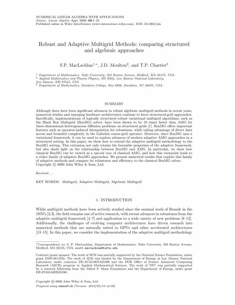
In the discussion that follows, we make use of a compass-based notation for connections inthe matrix, A, as given in Figure 1. In this notation, the row of the matrix equation Ax = bassociated with node (i, j) is given by
aSWi,j xi−1,j−1+aS
i,jxi,j−1 + aSEi,j xi+1,j−1 + aW
i,jxi−1,j + aOi,jxi,j
+aEi,jxi+1,j + aNW
i,j xi−1,j+1 + aNi,jxi,j+1 + aNE
i,j xi+1,j+1 = bi,j .
Within BoxMG, just as within AMG, the goal of the definition of interpolation is to faithfullyrepresent this equation for an error that yields a small residual, typically assumed to be zero:
aSWi,j ei−1,j−1+aS
i,jei,j−1 + aSEi,j ei+1,j−1 + aW
i,jei−1,j + aOi,jei,j
+aEi,jei+1,j + aNW
i,j ei−1,j+1 + aNi,jei,j+1 + aNE
i,j ei+1,j+1 = 0, (1)
although the inclusion of the residual in an affine interpolation process was noted to beimportant in certain cases in [17].
2.1. Classical BoxMG Interpolation
The classical BoxMG interpolation operator involves four cases:
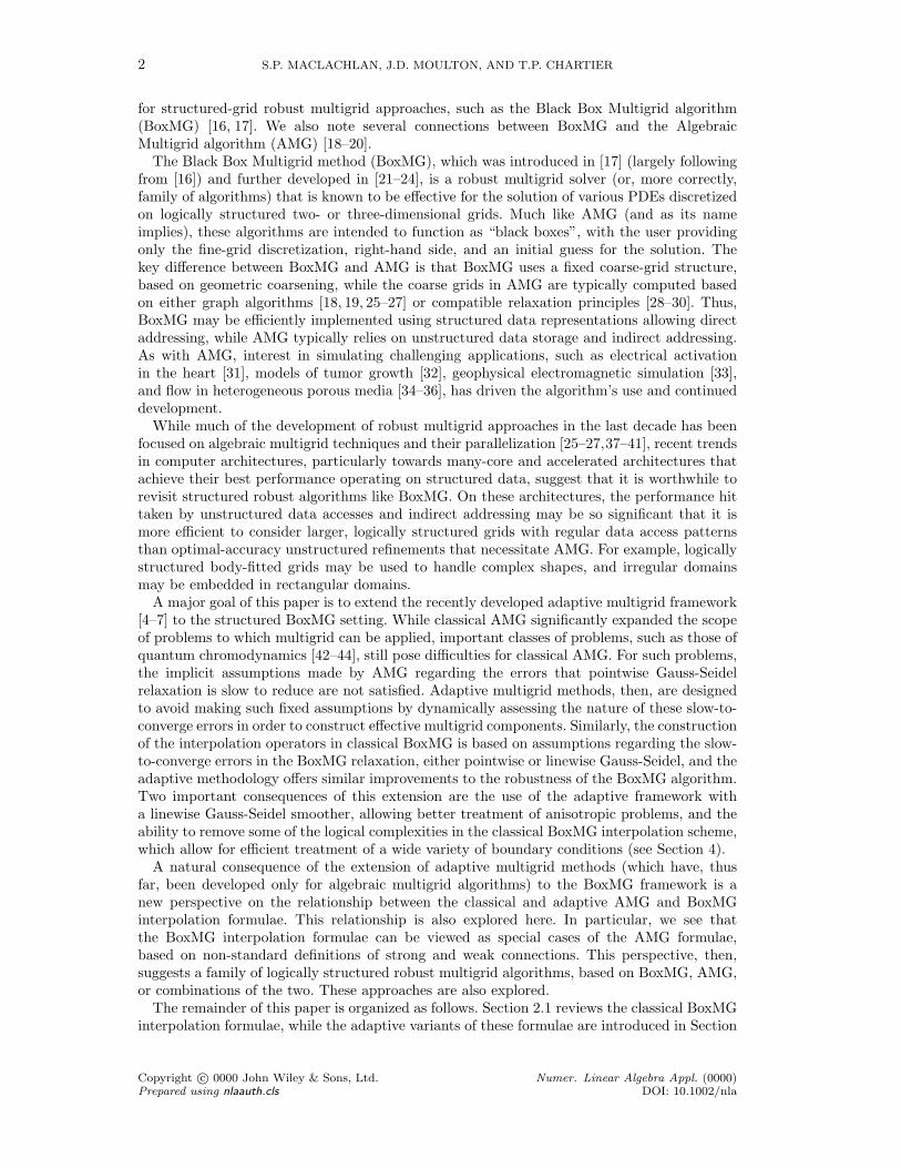
1. (i, j) is a coarse point: In this case, shown at the left of Figure 2, interpolation simplypreserves the coarse-grid value:
(PeC
)i,j
= eCI,J , where (I, J) is the coarse-grid index for
the node corresponding to (i, j) on the fine grid.2. (i− 1, j) and (i+ 1, j) are coarse points: In this case, shown in the middle of Figure
2, point (i, j) lies embedded in a coarse-grid line in the x-direction, and the goal isto define a one-dimensional interpolation formula from coarse-grid points (I, J) and(I + 1, J), corresponding to fine-grid points (i− 1, j) and (i+ 1, j), respectively, to (i, j).
Copyright c© 0000 John Wiley & Sons, Ltd. Numer. Linear Algebra Appl. (0000)Prepared using nlaauth.cls DOI: 10.1002/nla
4 S.P. MACLACHLAN, J.D. MOULTON, AND T.P. CHARTIER
................................
................................
....
....
....
....
....
....
....
....
................................
aOi,j
aNEi,jaNi,jaNWi,j
aEi,jaWi,j
aSi,j aSEi,jaSWi,j
Figure 1. Compass-Based Notation for the Stencil at Node (i, j)
Figure 2. The schematic [45] shows injection of coarse-grid points (left) and interpolation of twodifferent classes of fine-grid points: points embedded in coarse-grid lines (middle), and points located
at the logical center of a coarse-grid cell (right).
The BoxMG approach is to simply collapse the stencil in the y-direction onto the line withfixed y-coordinate, j. Thus, in Equation (1), we assume that the error is approximatelyconstant in the y direction and write
ek,j ≈ ek,j−1 ≈ ek,j+1, for k = i− 1, i, i+ 1, (2)
giving(aS
i,j + aOi,j + aN
i,j
)ei,j = −
(aSW
i,j + aWi,j + aNW
i,j
)eCI,J −
(aSE
i,j + aEi,j + aNE
i,j
)eCI+1,J , (3)
where we have used the injected errors at the coarse-grid points, ei−1,j = eCI,J and
ei+1,j = eCI+1,J . Thus, the interpolation formula is given by
(PeC)i,j = −aSW
i,j + aWi,j + aNW
i,j
aSi,j + aO
i,j + aNi,j
eCI,J −
aSEi,j + aE
i,j + aNEi,j
aSi,j + aO
i,j + aNi,j
eCI+1,J . (4)
Writing aOyi,j = aS
i,j + aOi,j + aN
i,j , aWi,j = aSW
i,j + aWi,j + aNW
i,j , and aEi,j = aSE
i,j + aEi,j + aNE
i,j ,
this can be compactly written as (PeC)i,j = − aWi,j
aOyi,j
eCI,J −
aEi,j
aOyi,j
eCI+1,J .
3. (i, j − 1) and (i, j + 1) are coarse points: This case is analogous to the previous one,with the roles of the x- and y-coordinates switched. Thus, taking (I, J) and (I, J + 1)to be the coarse-grid indices corresponding to fine-grid points (i, j − 1) and (i, j + 1),respectively, we make the approximations that
ei,k ≈ ei−1,k ≈ ei+1,k, for k = j − 1, j, j + 1.
Copyright c© 0000 John Wiley & Sons, Ltd. Numer. Linear Algebra Appl. (0000)Prepared using nlaauth.cls DOI: 10.1002/nla
ROBUST AND ADAPTIVE MULTIGRID METHODS 5
Substituting these in Equation (1) and rearranging, as above, gives
(PeC)i,j = −aSW
i,j + aSi,j + aSE
i,j
aWi,j + aO
i,j + aEi,j
eCI,J −
aNWi,j + aN
i,j + aNEi,j
aWi,j + aO
i,j + aEi,j
eCI,J+1. (5)
4. (i− 1, j − 1), (i+ 1, j − 1), (i− 1, j + 1), and (i+ 1, j + 1) are coarse points: In thiscase, shown at the right of Figure 2, the fine-grid point (i, j) lies at the center of a coarse-grid cell with nodes (I, J), (I + 1, J), (I, J + 1), and (I + 1, J + 1) corresponding to fine-grid nodes (i− 1, j − 1), (i+ 1, j − 1), (i− 1, j + 1), and (i+ 1, j + 1), respectively. Inthis case, there is no clear preferential geometric direction for collapsing the stencil, sinceeach connection to the fine-grid neighbors of (i, j) is equidistant (both geometrically andgrid-wise) from two coarse-grid points and (i, j) itself. However, as interpolation hasalready been determined for each of these neighbors, we can leverage the definitions ofinterpolation given above to eliminate them from Equation (1), writing
aSWi,j ei−1,j−1+aS
i,j
(PeC
)i,j−1
+ aSEi,j ei+1,j−1 + aW
i,j
(PeC
)i−1,j
+ aOi,jei,j
+aEi,j
(PeC
)i+1,j
+ aNWi,j ei−1,j+1 + aN
i,j
(PeC
)i,j+1
+ aNEi,j ei+1,j+1 = 0,
or
aOi,jei,j = −aSW
i,j eCI,J − aS
i,j
(PeC
)i,j−1
− aSEi,j e
CI+1,J − aW
i,j
(PeC
)i−1,j
(6)
−aEi,j
(PeC
)i+1,j
− aNWi,j eC
i,J+1 − aNi,j
(PeC
)i,j+1
− aNEi,j e
CI+1,I+1.
Denoting the coefficient of P interpolating from coarse-grid node (K,L) to fine-grid node(k, `) by p(k,`),(K,L) (in a slight modification of the usual row-column indexing notation),we can then expand the entries of PeC that appear above as(
PeC)i,j−1
= p(i,j−1),(I,J)eCI,J + p(i,j−1),(I+1,J)e
CI+1,J ,(
PeC)i,j+1
= p(i,j+1),(I,J+1)eCI,J+1 + p(i,j+1),(I+1,J+1)e
CI+1,J+1,(
PeC)i−1,j
= p(i−1,j),(I,J)eCI,J + p(i−1,j),(I,J+1)e
CI,J+1,
and(PeC
)i+1,j
= p(i+1,j),(I+1,J)eCI+1,J + p(i+1,j),(I+1,J+1)e
CI+1,J+1.
Making these substitutions into Equation (6) implicitly gives the interpolation formula
(PeC
)i,j
=−aSW
i,j + aSi,jp(i,j−1),(I,J) + aW
i,jp(i−1,j),(I,J)
aOi,j
eCI,J
−aSE
i,j + aSi,jp(i,j−1),(I+1,J) + aE
i,jp(i+1,j),(I+1,J)
aOi,j
eCI+1,J
−aNW
i,j + aNi,jp(i,j+1),(I,J+1) + aW
i,jp(i−1,j),(I,J+1)
aOi,j
eCI,J+1
−aNE
i,j + aNi,jp(i,j+1),(I+1,J+1) + aE
i,jp(i+1,j),(I+1,J+1)
aOi,j
eCI+1,J+1. (7)
To achieve added robustness, for problems on grids of dimensions other than 2N + 1, thatinclude lower-order terms, or that involve a wide variety of boundary conditions, the BoxMGalgorithm supplements these definitions with a heuristic switch for diagonally dominant rowsof the matrix [45]. Thus, each of the definitions in Equations (4), (5), and (7) has a generalizedform that makes use of this switch. For example, at fine-grid points embedded in horizontalcoarse-grid lines, Equation (4) becomes
(PeC)i,j = −aW
i,j
AOyi,j
eCI,J −
aEi,j
AOyi,j
eCI+1,J .
Copyright c© 0000 John Wiley & Sons, Ltd. Numer. Linear Algebra Appl. (0000)Prepared using nlaauth.cls DOI: 10.1002/nla
6 S.P. MACLACHLAN, J.D. MOULTON, AND T.P. CHARTIER
Taking AOyi,j = aOy
i,j , as in Equation (4) above, is referred to as averaging interpolation.Although this is an effective option for many situations, there are also situations wherethis leads to poor performance, particularly for diagonally dominant rows of the matrix.An alternate approach, defining AOy
i,j = aWi,j + aE
i,j , gives interpolation coefficients that exactlypreserve the constant in interpolation, even when the stencil is diagonally dominant. Thisformulation is referred to as constant-preserving interpolation; although this approach iseffective in many situations, it is not always successful. Most notably, constant-preservinginterpolation fails when the grids are not of dimension 2N + 1 in each direction, asextrapolation is used at the right and/or top boundaries.
The solution implemented in BoxMG is to use a heuristic switch to choose between these twoformulations. Letting ωy = aW
i,j + aEi,j , the denominator of the interpolation weights is defined
as,
AOyi,j =
aOy
i,j aOi,j > (1 + εy)ωy
ωy aOi,j ≤ (1 + εy)ωy
,
where εy = min(|aWi,j |/aO
i,j , |aEi,j |/aO
i,j). An analogous switch is defined for the fine-grid pointsembedded in y-lines, and for fine-grid points in the interior of coarse-grid cells. This formulationis referred to as switched interpolation.
2.2. Adaptive BoxMG interpolation
Adjusting the interpolation formulae in Equations (4), (5), and (7) to account for modifiedinformation about the near-null space of matrix A can be done following a similar approach asin [6]. In (4) and (5), connections between the fine-grid point (i, j) and its fine-grid neighborsare collapsed based on the assumption that the unwanted values of the fine-grid error vectorcould be accurately approximated directly by the values at their neighbors on the coarse grid,or by the error at point (i, j) itself. This is a natural assumption when the matrix, A, comesfrom a standard discretization of an elliptic differential operator, for which the constant vectorgives a good local representative of the near-null space of the matrix. As such, this is closelyrelated to the standard AMG assumption that algebraically smooth errors vary slowly alongstrong connections [18].
When the constant vector doesn’t give a good representation of the near-null space of thematrix, adaptive multigrid methods [4–6, 11, 47–50] make use of so-called prototype vectors,that are assumed to give an accurate local picture of the variation in the near-null spaceof the matrix or, equivalently, in the slow-to-converge errors for simple pointwise relaxationschemes, such as weighted Jacobi or Gauss-Seidel. Because we consider such adaptivity withinthe setting of the scalar BoxMG algorithm (and, in particular, not its systems variant [22]),we only consider the case where such information is provided in the form of a single prototypevector, z, although recent experience with the scalar gauged-Laplacian operator from quantumchromodynamics suggests that this may limit the applicability of the resulting algorithm [47].
Thus, given a single prototype vector, z, we propose to modify the interpolation rules givenin Equations (4) and (5) based on indirect fitting of z. When point (i, j) is embedded in acoarse-grid line in the x-direction, instead of making the approximations in Equation (2) thatlead to (4), we define local scaling factors based on the prototype,
wSk,j =
zk,j−1
zk,jand wN
k,j =zk,j+1
zk,j, for k = i− 1, i, i+ 1,
and make weighted approximations to the error in the y direction,
ek,j−1 ≈ wSk,jek,j and ek,j+1 ≈ wN
k,jek,j , for k = i− 1, i, i+ 1.
These factors locally capture the slope of the error transverse to the direction of interpolation,leading to the definition of a rich interpolation space that appropriately represents theprototype vector. With these approximations, the overall approximation of Equation (1)
Copyright c© 0000 John Wiley & Sons, Ltd. Numer. Linear Algebra Appl. (0000)Prepared using nlaauth.cls DOI: 10.1002/nla
ROBUST AND ADAPTIVE MULTIGRID METHODS 7
becomes (wS
i,jaSi,j + aO
i,j + wNi,ja
Ni,j
)ei,j =−
(wS
i−1,jaSWi,j + aW
i,j + wNi−1,ja
NWi,j
)eCI,J
−(wS
i+1,jaSEi,j + aE
i,j + wNi+1,ja
NEi,j
)eCI+1,J ,
which gives the interpolation formula,
(PeC)i,j = −wS
i−1,jaSWi,j + aW
i,j + wNi−1,ja
NWi,j
wSi,ja
Si,j + aO
i,j + wNi,ja
Ni,j
eCI,J −
wSi+1,ja
SEi,j + aE
i,j + wNi+1,ja
NEi,j
wSi,ja
Si,j + aO
i,j + wNi,ja
Ni,j
eCI+1,J .
Rewriting this in terms of only entries in A and z gives
(PeC)i,j =−zi,j
(aSW
i,j zi−1,j−1 + aWi,jzi−1,j + aNW
i,j zi−1,j+1
)zi−1,j
(aS
i,jzi,j−1 + aOi,jzi,j + aN
i,jzi,j+1
) eCI,J (8)
−zi,j
(aSE
i,j zi+1,j−1 + aEi,jzi+1,j + aNE
i,j zi+1,j+1
)zi+1,j
(aS
i,jzi,j−1 + aOi,jzi,j + aN
i,jzi,j+1
) eCI+1,J .
Similarly, to replace the interpolation formula given in Equation (5) for the case where point(i, j) is embedded in a coarse-grid line in the y-direction, we define the scaling factors,
wWi,k =
zi−1,k
zi,kand wE
i,k =zi+1,k
zi,k, for k = j − 1, j, j + 1,
and make weighted approximations to the error in the x direction,
ei−1,k ≈ wWi,kei,k and ei+1,k ≈ wE
i,kei,k, for k = j − 1, j, j + 1.
Then, following the analogous derivation as in Equation (8), we can derive the adaptive versionof Equation (5),
(PeC)i,j = −wW
i,j−1aSWi,j + aS
i,j + wEi,j−1a
SEi,j
wWi,ja
Wi,j + aO
i,j + wEi,ja
Ei,j
eCI,J −
wWi,j+1a
NWi,j + aN
i,j + wEi,j+1a
NEi,j
wWi,ja
Wi,j + aO
i,j + wEi,ja
Ei,j
eCI,J+1.
Again rewriting in terms of the entries of A and z gives
(PeC)i,j =−zi,j
(aSW
i,j zi−1,j−1 + aSi,jzi,j−1 + aSE
i,j zi+1,j−1
)zi,j−1
(aW
i,jzi−1,j + aOi,jzi,j + aE
i,jzi+1,j
) eCI,J (9)
−zi,j
(aNW
i,j zi−1,j+1 + aNi,jzi,j+1 + aNE
i,j zi+1,j+1
)zi,j+1
(aW
i,jzi−1,j + aOi,jzi,j + aE
i,jzi+1,j
) eCI,J+1.
While modification of the definition of interpolation to fine-grid nodes that lie at the centersof coarse-grid cells, as given in (6), is possible (see Section 3), it is natural to keep the generalform, and simply replace the values of
(PeC
)i,j−1
,(PeC
)i,j+1
,(PeC
)i−1,j
, and(PeC
)i+1,j
with those from Equations (8) and (9).An immediate consequence of these definitions is a scaling-invariance property of the
adaptive BoxMG interpolation scheme given in Equations (8) and (9). Just as in classicalAMG [6], the performance of classical BoxMG is known to suffer significantly when the systemmatrix, A, is rescaled, even in the simplest ways; however, the adjustments in (8) and (9) aresufficient to “undo” the effects of scaling.
Theorem 1. Let A be a given matrix with regular 9-point connectivity structure (i.e., anon-zero pattern contained within that of the standard 9-point tensor-product bilinear finite-element stencil on a regular mesh), and let S be a non-singular diagonal matrix. DefineA = SAS, and z = S−11 to be the prototype vector for adaptive BoxMG interpolation, sothat zi,j = 1/s(i,j),(i,j) is the value of the prototype at node (i, j). Let P denote the classical
Copyright c© 0000 John Wiley & Sons, Ltd. Numer. Linear Algebra Appl. (0000)Prepared using nlaauth.cls DOI: 10.1002/nla
8 S.P. MACLACHLAN, J.D. MOULTON, AND T.P. CHARTIER
BoxMG interpolation operator for matrix A, as given in Equations (4), (5), and (7). Assumethat all of
aOi,j
aWi,j + aO
i,j + aEi,j
aSi,j + aO
i,j + aNi,j
aWi,jzi−1,j + aO
i,jzi,j + aEi,jzi+1,j
aSi,jzi,j−1 + aO
i,jzi,j + aNi,jzi,j+1
are nonzero for each node (i, j) where these appear in the interpolation formulae, so thatboth the classical BoxMG interpolation operator for A and the adaptive BoxMG interpolationoperator for A based on prototype z, P , are well-defined. Then, P = S−1PSc, where Sc is thediagonal matrix whose values are given by taking the values of S at only the coarse-grid nodes.
ProofWe prove this result by considering each of the four cases discussed above.
1. (i, j) is a coarse point: In this case, both(PeC
)i,j
= eCI,J and
(PeC
)i,j
= eCI,J . Note,
however, that the entry on the diagonal of Sc corresponding to (I, J) is the same as theentry on the diagonal of S corresponding to (i, j), so that the effects of the left and rightscalings in S−1PSc on these rows cancel out.
2. (i− 1, j) and (i+ 1, j) are coarse points: In this case, we have two formulae for theclassical and adaptive cases, Equations (4) and (8), respectively, giving
(PeC)i,j =−aSW
i,j + aWi,j + aNW
i,j
aSi,j + aO
i,j + aNi,j
eCI,J −
aSEi,j + aE
i,j + aNEi,j
aSi,j + aO
i,j + aNi,j
eCI+1,J
and (PeC)i,j =−zi,j
(aSW
i,j zi−1,j−1 + aWi,jzi−1,j + aNW
i,j zi−1,j+1
)zi−1,j
(aS
i,jzi,j−1 + aOi,jzi,j + aN
i,jzi,j+1
) eCI,J
−zi,j
(aSE
i,j zi+1,j−1 + aEi,jzi+1,j + aNE
i,j zi+1,j+1
)zi+1,j
(aS
i,jzi,j−1 + aOi,jzi,j + aN
i,jzi,j+1
) eCI+1,J .
Noting that the scaling, A = SAS, gives aSWi,j = aSW
i,j z−1i,j z
−1i−1,j−1, aW
i,j = aWi,jz−1i,j z
−1i−1,j ,
and so forth, we see that many of the terms, zk,`, in the adaptive case cancel with thescaling in A, ultimately giving
PeCi,j = −
zi,j
(aSW
i,j + aWi,j + aNW
i,j
)zi−1,j
(aS
i,j + aOi,j + aN
i,j
) eCI,J −
zi,j
(aSE
i,j + aEi,j + aNE
i,j
)zi+1,j
(aS
i,j + aOi,j + aN
i,j
)eCI+1,J .
From this, we see that p(i,j),(I,J) = zi,j
zi−1,jp(i,j),(I,J) and that p(i,j),(I+1,J) =
zi,j
zi+1,jp(i,j),(I+1,J). Further noting that the entry of Sc corresponding to (I, J) is z−1
i−1,j
and that corresponding to (I + 1, J) is z−1i+1,j (since (i− 1, j) and (i+ 1, j) are the
fine-grid points corresponding to these coarse-grid indices), establishes that p(i,j),(I,J) =(S−1PSc
)(i,j),(I,J)
and p(i,j),(I+1,J) =(S−1PSc
)(i,j),(I+1,J)
.3. (i, j − 1) and (i, j + 1) are coarse points: This case is essentially identical to the
previous case, except that we now identify coarse points (I, J) and (I, J + 1) with finepoints (i, j − 1) and (i, j + 1), respectively. Following the analogous steps, Equation (9)becomes
(PeC)i,j = −zi,j
(aSW
i,j + aSi,j + aSE
i,j
)zi,j−1
(aW
i,j + aOi,j + aE
i,j
)eCI,J −
zi,j
(aNW
i,j + aNi,j + aNE
i,j
)zi,j+1
(aW
i,j + aOi,j + aE
i,j
) eCI,J+1.
Copyright c© 0000 John Wiley & Sons, Ltd. Numer. Linear Algebra Appl. (0000)Prepared using nlaauth.cls DOI: 10.1002/nla
ROBUST AND ADAPTIVE MULTIGRID METHODS 9
As before, we see the relationship that p(i,j),(I,J) = zi,j
zi,j−1p(i,j),(I,J) and p(i,j),(I,J+1) =
zi,j
zi,j+1p(i,j),(I,J+1); a similar argument shows that p(i,j),(I,J) =
(S−1PSc
)(i,j),(I,J)
and
p(i,j),(I,J+1) =(S−1PSc
)(i,j),(I,J+1)
.4. (i− 1, j − 1), (i+ 1, j − 1), (i− 1, j + 1), and (i+ 1, j + 1) are coarse points: In this
case, the formula for A follows that for A, with entries from P replacing those of P :(PeC
)i,j
=−aSW
i,j + aSi,j p(i,j−1),(I,J) + aW
i,j p(i−1,j),(I,J)
aOi,j
eCI,J
−aSE
i,j + aSi,j p(i,j−1),(I+1,J) + aE
i,j p(i+1,j),(I+1,J)
aOi,j
eCI+1,J
−aNW
i,j + aNi,j p(i,j+1),(I,J+1) + aW
i,j p(i−1,j),(I,J+1)
aOi,j
eCI,J+1
−aNE
i,j + aNi,j p(i,j+1),(I+1,J+1) + aE
i,j p(i+1,j),(I+1,J+1)
aOi,j
eCI+1,J+1,
where the coarse-grid indices (I, J), (I + 1, J), (I, J + 1), and (I + 1, J + 1) refer tofine-grid points (i− 1, j − 1), (i+ 1, j − 1), (i− 1, j + 1), and (i+ 1, j + 1), respectively.Making the appropriate substitutions for entries in A and P , we have
p(i,j),(I,J) = −aSW
i,j + aSi,j p(i,j−1),(I,J) + aW
i,j p(i−1,j),(I,J)
aOi,j
= −aSW
i,j z−1i,j z
−1i−1,j−1
aOi,jz−2i,j
−aS
i,jz−1i,j z
−1i,j−1p(i,j−1),(I,J)
zi,j−1zi−1,j−1
aOi,jz−2i,j
−aW
i,jz−1i,j z
−1i−1,jp(i−1,j),(I,J)
zi−1,j
zi−1,j−1
aOi,jz−2i,j
= −zi,j
(aSW
i,j + aSi,jp(i,j−1),(I,J) + aW
i,jp(i−1,j),(I,J)
)zi−1,j−1aO
i,j
=zi,j
zi−1,j−1p(i,j),(I,J).
Similar calculations for the other coefficients show that
p(i,j),(I+1,J) =zi,j
zi+1,j−1p(i,j),(I+1,J),
p(i,j),(I,J+1) =zi,j
zi−1,j+1p(i,j),(I,J+1),
and p(i,j),(I+1,J+1) =zi,j
zi+1,j+1p(i,j),(I+1,J+1).
As before, this shows that these coefficients are also scaled as given by P = S−1PSc.
The desired corollary to Theorem 1 is that the performance of BoxMG based on adaptiveinterpolation applied to Ax = b is equivalent to that of classical BoxMG applied to Ax = b;however, the truth of this depends on both the choice of smoother and availability of entries inS. If the error-propagation operator for the BoxMG smoother applied to A is I −MA, whilethat applied to A is I − MA, then the performance of BoxMG based on adaptive interpolationapplied to Ax = b depends on how M relates to S. For standard smoothers, such as Jacobi andGauss-Seidel, M−1 = SM−1S and, so, I − MA = S−1(I −MA)S. The same relation holds forline smoothers, or any other smoother where M−1 is chosen by taking a fixed subset of thenonzero elements of A. Under the assumption that M−1 = SM−1S, it can be seen that theoverall solver performance of BoxMG based on adaptive interpolation applied to Ax = b is
Copyright c© 0000 John Wiley & Sons, Ltd. Numer. Linear Algebra Appl. (0000)Prepared using nlaauth.cls DOI: 10.1002/nla
10 S.P. MACLACHLAN, J.D. MOULTON, AND T.P. CHARTIER
equivalent to that of classical BoxMG applied to Ax = b, when the diagonal scaling S is knownexactly. This, of course, is not a practical assumption, although results in Section 4 show thata good enough approximation can usually be found such that the performance doesn’t suffervery much.
2.3. Adaptive setup procedure
In this paper, we make use of a simple adaptive setup cycling scheme, as was consideredin [6], where the prototype vector is initialized to be a random vector, and an initial series ofsetup V-cycles is performed. On each level of these cycles, a fixed number of pre-relaxations isperformed on the homogeneous problem, Az = 0 (with the current prototype on that level usedas the initial guess), an adaptive interpolation operator, P , is formed based on the resultingimproved prototype, which is then injected to give an initial prototype vector on the nextcoarser grid along with the computed Galerkin coarse-grid operator, PTAP . After these steps,the process moves to the next coarser grid and begins again, until the coarsest grid is reached.No computation is done on the coarsest grid (although further relaxation or an exact eigensolvemight be used to improve the process [6, 7, 49]). On the upward traversal of the V-cycle, thecoarser-grid prototype is interpolated to the finer grid based on the appropriate adaptiveinterpolation operator defined on the downward traversal, again a fixed number of relaxationson Az = 0 is performed with the interpolated prototype as the initial guess, but no updateis computed for the interpolation operators. (Thus, if we are performing a fixed number ofcycles, we skip this relaxation on the final cycle to avoid unnecessary work.) As was notedin [6], this is not typically the most efficient approach to the adaptive cycling when only oneor two relaxations are used on each level in the setup V-cycle, as we consider in Section 4;rather, this serves to illustrate the overall performance of the adaptive approach.
After these setup cycles are performed, we take the interpolation and Galerkin coarse-gridoperators defined on the last adaptive cycle and use these in the solve phase of the algorithm.The solve phase makes use of standard multigrid V-cycles in the usual way. Here, we follow theBoxMG solution algorithm and make use of either pointwise or linewise Gauss-Seidel relaxationand Galerkin coarse-grid correction.
3. CONNECTIONS BETWEEN BOXMG AND AMG
The equivalence given in Theorem 1 is effectively the same as that observed for classical andadaptive AMG in [6], and relies on similar cancellations occurring when the scaled coefficientsof A are introduced into the adaptive interpolation formula. Thus, it is natural to investigatethe connection between both the classical and adaptive interpolation formulae for BoxMGand AMG. Here, we show that BoxMG can be viewed as a “special case” of AMG, based ongeometric choices of the definitions of strong connections, rather than the typical algebraicchoice based on classical M-matrix properties [18].
The primary difference between the coarsening algorithms employed by BoxMG and AMGis in the selection of coarse grids, with BoxMG using standard geometric coarsening, whileAMG uses an algebraic approach based on the graph of the matrix, A, filtered based on“strong connections”. If A has a standard 9-point stencil with all connections deemed tobe strong, then the standard “fully coarsened” grid used by BoxMG is an allowable coarsegrid for the classical AMG coloring algorithm [51]. While this standard coarsening can alsoarise in other situations, our goal here is, instead, to examine the interpolation processesrather than the coarse-grid selection algorithms. However, it is interesting to note some ofthe fundamental differences between BoxMG and AMG that result from these very differentapproaches to coarsening. First, since BoxMG uses a geometric coarsening that is independentof the problem, some fine-scale features of the problem, such as discontinuities in the continuumdiffusion coefficients, will not be preserved on coarser grids. In these cases, the operator-inducedinterpolation must capture these features and, through the Galerkin coarse-grid operator,
Copyright c© 0000 John Wiley & Sons, Ltd. Numer. Linear Algebra Appl. (0000)Prepared using nlaauth.cls DOI: 10.1002/nla
ROBUST AND ADAPTIVE MULTIGRID METHODS 11
represent their influence on coarser grids. In contrast, the algebraic approach to coarseningin classical AMG naturally attempts to preserve these features on coarser grids and, hence,tends to coarsen along features but not across them. Similarly, for anisotropic problems, AMGaims to achieve the semicoarsened grids needed for efficient multigrid solution using pointwisesmoothers, while BoxMG defaults to using the coupled line relaxation (and, in 3D, planerelaxation) approaches needed for efficient multigrid solution using full geometric coarsening.
Based on this structured coarse grid, the BoxMG interpolation formulae are given abovein Section 2. In contrast, the AMG interpolation formulae are determined based on only twocases, when a fine-grid point is also a coarse-grid point, and when it isn’t. When node (i, j)is both a fine-grid and coarse-grid point, then the AMG interpolation is the same as BoxMG,(PeC
)i,j
= eCI,J , where (I, J) is the coarse-grid index corresponding to fine-grid point (i, j).
When (i, j) doesn’t correspond to a coarse-grid point, the definition of AMG interpolationbegins with the same small-residual assumption that gives Equation (1). From here, theneighboring points, indexed by d ∈ SW,S, SE,W,E,NW,N,NE, are divided into thestrongly connected coarse-grid, Ci,j , and fine-grid, Fi,j , neighbors and the weakly connectedneighbors, Wi,j . Then, Equation (1) can be rewritten as
aOi,jei,j = −
∑d∈Ci,j
adi,je(i,j)+~d −
∑d′∈Fi,j
ad′
i,je(i,j)+~d′ −∑
d′′∈Wi,j
ad′′
i,je(i,j)+~d′′ ,
where we use the notation e(i,j)+~d to denote the error at the grid point in direction d from
(i, j); for example, e(i,j)+
−−→SW
= ei−1,j−1. For directions d ∈ Ci,j , node (i, j) + ~d is a coarse-gridnode, and so these values can be used directly in interpolation. The goal in the AMG definitionof interpolation is to “collapse” connections to d ∈ Fi,j ∪Wi,j onto those in Ci,j .
Weak connections, d′′ ∈Wi,j , occur when ad′′
i,j is small enough that the approximation ofe(i,j)+~d′′ is unimportant, so long as a significant error in scaling isn’t made. In this case, itis typical to assume that e(i,j)+~d′′ ≈ ei,j , so that the connection is said to be collapsed ontothe diagonal. For strong connections between (i, j) and one of its fine-grid neighbors, d′ ∈ Fi,j ,AMG interpolation makes the approximation that the error at node (i, j) + ~d′ can be writtenas a linear combination of the errors at the coarse-grid points d ∈ Ci,j ,
e(i,j)+~d′ ≈∑
d∈Ci,j
wd′,di,j e(i,j)+~d.
To determine the coefficients, wd′,di,j , we again start with a modified form of Equation (1),
aO(i,j)+~d′
e(i,j)+~d′ = −∑
d∈Ci,j
ad−d′
(i,j)+~d′e(i,j)+~d −
∑d′′ /∈Ci,j∪d′
ad′′−d′
(i,j)+~d′e(i,j)+~d′′ , (10)
where the notation d− d′ refers to the net direction between nodes (i, j) + ~d′ and (i, j) + ~d,when d′ and d are directions measured from node (i, j). For example, if d′ = SW and d = W ,then d− d′ = N , the direction from (i− 1, j − 1) to (i− 1, j). Note that d− d′ is not well-defined for all pairs of directions (e.g., if d′ = SW and d = N); the coefficient ad−d′
(i,j)+~d′is taken
to be zero if d− d′ is not well defined.To turn Equation (10) into an interpolation weighting to collapse the connection to ad′
i,j , weintroduce an approximation, where the second sum on the right-hand side is discarded, andthe coefficient of e(i,j)+~d′ is modified to compensate. In classical AMG, this is done based onthe assumption that the slow-to-converge errors of relaxation (the algebraically smooth errors)locally match the constant vector, so that the interpolation from d ∈ Ci,j to (i, j) + ~d′ shouldalso preserve the constant vector. With this assumption, the weights wd′,d
i,j for d ∈ Ci,j are
Copyright c© 0000 John Wiley & Sons, Ltd. Numer. Linear Algebra Appl. (0000)Prepared using nlaauth.cls DOI: 10.1002/nla
12 S.P. MACLACHLAN, J.D. MOULTON, AND T.P. CHARTIER
given by
wd′,di,j =
ad−d′
(i,j)+~d′∑d′′∈Ci,j
ad′′−d′
(i,j)+~d′
. (11)
Putting these all together gives the approximation of Equation (1) ofaOi,j +
∑d′′∈Wi,j
ad′′
i,j
ei,j = −∑
d∈Ci,j
adi,je(i,j)+~d −
∑d′∈Fi,j
ad′
i,j
∑d∈Ci,j
ad−d′
(i,j)+~d′∑d′′∈Ci,j
ad′′−d′
(i,j)+~d′
e(i,j)+~d,
(12)which can easily be transformed into an interpolation operator after consolidating terms onthe right-hand side and dividing by the coefficient on the left-hand side.
While Equation (12) and its derivation appear to be completely unrelated to the BoxMGformulae derived in Section 2, there are, nonetheless, similarities in the treatment ofconnections from node (i, j) to fine-grid neighbors in Equation (1). Considering Equation (3),we see that this has similar form, with the term aS
i,j + aOi,j + aN
i,j replacing the sum on the left-hand side, and simple sums of coefficients on the right-hand side. Note, however, that in thiscase, nodes (i+ 1, j + 1) and (i+ 1, j − 1) have only a single connection to d ∈ Ci,j , for d = E,so that wNE,E
i,j = wSE,Ei,j = 1 and, similarly, wNW,W
i,j = wSW,Wi,j = 1. Thus, one observation is
that the BoxMG interpolation formula in Equation (4) is the same as the AMG interpolationformula in this case, where nodes (i, j ± 1) are treated as weakly connected neighbors(S,N ∈Wi,j), and (i− 1, j ± 1) and (i+ 1, j ± 1) are treated as strongly connected fine-gridneighbors (SW,NW,SE,NE ∈ Fi,j), with (i± 1, j) as coarse-grid neighbors, W,E ∈ Ci,j .
This equivalence is, however, somewhat unsatisfactory, as there is no apparent justificationin treating the connections to nodes (i, j ± 1) as weak connections. A more satisfying point ofview arises from considering an analogue of Equation (10) in which collapsing strong fine-gridconnections is allowed to both (i, j) and d ∈ Ci,j :
aO(i,j)+~d′
e(i,j)+~d′ = −∑
d∈Ci,j∪O
ad−d′
(i,j)+~d′e(i,j)+~d −
∑d′′ /∈Ci,j∪O,d′
ad′′−d′
(i,j)+~d′e(i,j)+~d′′ ,
leading to the analogue of Equation (11) for d ∈ Ci,j ∪ O,
wd′,di,j =
ad−d′
(i,j)+~d′∑d′′∈Ci,j∪O
ad′′−d′
(i,j)+~d′
.
With this definition of wd′,di,j , the modified AMG interpolation weights and the classical BoxMG
interpolation weights coincide when the definition of strong connections used in determining theAMG interpolation weights is based on the simple criterion of geometric distance. For each fine-grid neighbor of (i, j), (k, `), we say that (k, `) strongly depends on node (k′, `′) ∈ Ci,j ∪ (i, j)if and only if the geometric distance between (k, `) and (k′, `′) is minimal over all points inCi,j ∪ (i, j). Note that we specifically use geometric distance here rather than graph distance,since the two are not the same for a standard 9-point stencil. A similar conclusion holds forthe analogue of Equation (5).
For the case where (i, j) is in the center of a coarse-grid cell, given in Equation (7),the inclusion of node (i, j) in the distribution does not give equivalence between the AMGand BoxMG approaches. The “usual” indirect interpolation weights, given by Equation (11)may give this equivalence, depending on the relationship between the weights prescribed byEquation (11) and the BoxMG weights given in Equations (4) and (5). When these weightsare the same (as, for instance, they will be in cases where both result in linear interpolationalong cell edges, such as for a constant-coefficient diffusion problem), then the BoxMG and
Copyright c© 0000 John Wiley & Sons, Ltd. Numer. Linear Algebra Appl. (0000)Prepared using nlaauth.cls DOI: 10.1002/nla
ROBUST AND ADAPTIVE MULTIGRID METHODS 13
AMG interpolation rules coincide. A plausible rule to distinguish between the cases where(i, j) should and shouldn’t be included in the distribution is based on whether or not node(k, `) is strongly connected (based on geometric distance) to only node (i, j) or to some nodesin Ci,j . When the strong connection is only to node (i, j), as in the horizontal and verticalline interpolation cases, the generalized formula should be used, since the denominator in theclassical formula (Equation (11)) is zero. This occurs because the fully coarsened grid enforcedby BoxMG violates the typical AMG assumption that every pair of strongly connected fine-grid points should have a common coarse-grid neighbor that is strongly connected to eachof the fine-grid points. When this assumption is not violated, as in the case when (i, j) is acoarse-grid cell center, the classical AMG collapsing should be used.
This connection between BoxMG and AMG is, to our knowledge, a new perspective on thesetwo robust multigrid approaches. While BoxMG has long been acknowledged as an efficientand robust multigrid solution algorithm, outperforming AMG by a factor of 10 in solving 3Dheterogeneous diffusion equations in [1], this connection provides the opportunity to investigatea broader family of structured robust multigrid methods, in both the classical and adaptiveframeworks. Among the possible “hybrid” approaches of structured coarsening with algebraicinterpolation are
1. Using classical or adaptive AMG interpolation on structured coarsening meshes,2. Using classical or adaptive AMG interpolation for interpolation along coarse-grid cell
edges, in place of Equations (4) and (5), combined with BoxMG interpolation for coarse-grid cell centers, and
3. Using classical or adaptive BoxMG interpolation for interpolation along coarse-grid celledges, combined with classical or adaptive AMG interpolation for coarse-grid cell centers.
In all of these cases, because of the explicit grid structure, we can derive fully explicit formulaeif we use geometric or graph-based definitions of strength of connection. Even with algebraicdefinitions of strength of connection, however, we can still make use of the known coarseningstructure to make use of direct data access in achieving significant speedup over naıve AMGimplementations. These hybrid approaches are investigated in Section 4.1.2.
4. NUMERICAL RESULTS
In this section, we explore the performance of adaptive BoxMG interpolation operators,in comparison to the classical BoxMG algorithm, as well as with interpolation based onAMG and adaptive AMG principles. We consider two examples where the fine-grid matrixcomes from a bilinear finite-element discretization of the second-order form of Darcy’s Law,−∇ · K(x)∇p(x) = q(x) on [0, 1]2, with variable permeability K(x). In the first examples, K(x)has a simple two-scale periodic structure that allows easy comparison and analysis of thenumerical performance of these algorithms. The second set of examples are more realistic, usinga geostatistical approach to generate layered media, with corresponding values of K(x). Finally,we consider test problems based on five-point finite-difference discretizations of both isotropicand anisotropic diffusion problems, with a focus on the effects of non-standard boundaryconditions.
4.1. Periodic Permeability
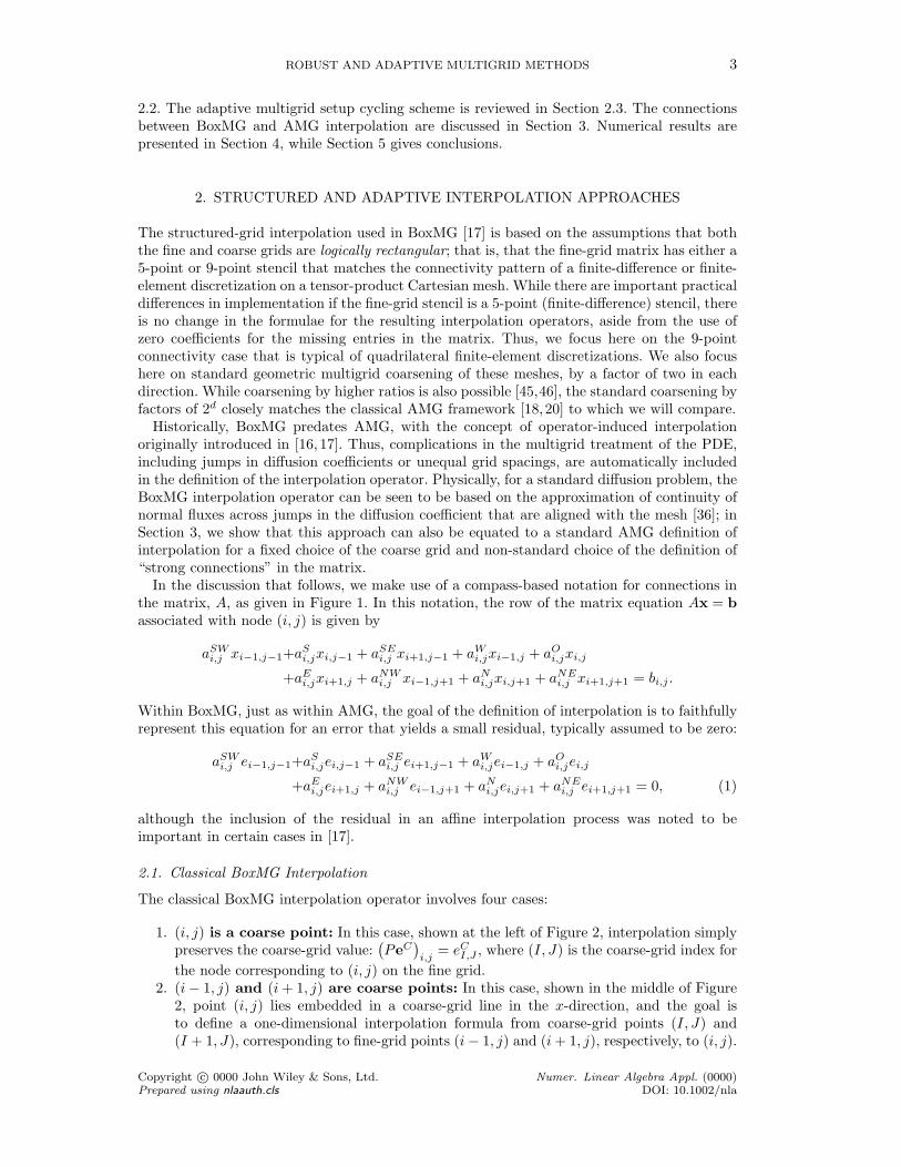
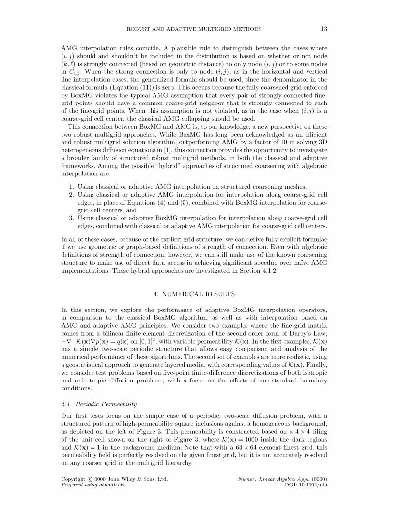
Our first tests focus on the simple case of a periodic, two-scale diffusion problem, with astructured pattern of high-permeability square inclusions against a homogeneous background,as depicted on the left of Figure 3. This permeability is constructed based on a 4× 4 tilingof the unit cell shown on the right of Figure 3, where K(x) = 1000 inside the dark regionsand K(x) = 1 in the background medium. Note that with a 64× 64 element finest grid, thispermeability field is perfectly resolved on the given finest grid, but it is not accurately resolvedon any coarser grid in the multigrid hierarchy.
Copyright c© 0000 John Wiley & Sons, Ltd. Numer. Linear Algebra Appl. (0000)Prepared using nlaauth.cls DOI: 10.1002/nla
14 S.P. MACLACHLAN, J.D. MOULTON, AND T.P. CHARTIER
1
05/16
5/16
11/16
1
111/160
0
1
0
Figure 3. Periodic permeability field. At left, the 4× 4 tiling of a unit cell (shown at right) that isused in the numerical examples that follow.
4.1.1. Neumann Boundary Conditions A natural first experiment is to see if the adaptiveBoxMG approach can recover the performance seen by the classical BoxMG approach in thecase where the ideal prototype vector is the constant vector. While classical BoxMG andAMG effectively use the constant vector as the prototype for all problems, in the adaptivesetup stage (regardless of the final choice of adaptive interpolation), the constant vector arisesas the ideal prototype only if it is the (unique) eigenvector associated with the largest (inmodulus) eigenvalue of the relaxation process. A natural way to guarantee that this is the caseis to consider the singular problem that arises from considering Neumann boundary conditionson all edges of the domain. The (unique) zero eigenvalue of the system matrix, A, becomesthe (unique) unit eigenvalue of the semi-convergent relaxation process, I −MA, for standardchoices of M , such as in weighted Jacobi or Gauss-Seidel relaxation. This, then, in the adaptiveviewpoint, makes the associated eigenvector (the constant vector) the ideal vector on whichto base interpolation.
The obvious disadvantage of considering the case with only Neumann Boundary conditionsis the singularity of the resulting linear system, and its effect on the convergence of theresulting multigrid V-cycle iteration. To address this, we employ two strategies. Followingclassical BoxMG [24], for problems with a non-zero right-hand side (i.e., in the case wherewe are interested in the solution of a PDE and not in measuring asymptotic convergencefactors), the singularity is treated only on the coarsest grid. Here, we modify the last diagonalentry of the coarsest-grid matrix to make it artificially non-singular before factoring it; aftersolving this perturbed coarsest-grid system in each V-cycle, we add a projection step, makingthe coarsest-grid correction orthogonal to the coarsest-grid constant vector, to ensure thatthe coarse-grid correction process does not introduce components in the direction of the nullspace. For the case of a non-zero right-hand side, this approach is sufficient to restore optimalmultigrid convergence to the level of machine precision; however, it does not allow for testingof asymptotic convergence rates by applying the multigrid V-cycle to a problem with a zeroright-hand side (with a random initial guess). In that case, we add an additional projectionstep against the finest-grid constant vector, to eliminate the effects of the singularity on themeasurement of the performance of the resulting multigrid methods. We note that both ofthese approaches rely on the assumption that the null-space vector is known with sufficientaccuracy to make these projections effective. In the case of the projection on the coarsest-grid,this means that the pre-image of the finest-grid null-space is assumed to be known; this maybe reasonable for standard finite-element problems, such as are typically considered, but addsan additional challenge for problems where this is not the case.
Our first test is to examine how the adaptive process converges to a steady-state, and howthat convergence can be related to the case of classical BoxMG. In Table I, we compare the
Copyright c© 0000 John Wiley & Sons, Ltd. Numer. Linear Algebra Appl. (0000)Prepared using nlaauth.cls DOI: 10.1002/nla
ROBUST AND ADAPTIVE MULTIGRID METHODS 15
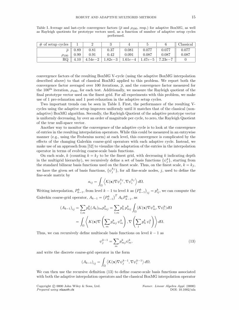
Table I. Average and last-cycle convergence factors (ρ and ρ100, resp.) for adaptive BoxMG, as wellas Rayleigh quotients for prototype vectors used, as a function of number of adaptive setup cycles
performed.
# of setup cycles 1 2 3 4 5 6 Classicalρ 0.89 0.81 0.37 0.081 0.077 0.077 0.077
ρ100 0.99 0.91 0.42 0.091 0.087 0.087 0.087RQ 4.10 4.54e−2 1.82e−3 1.61e−4 1.47e−5 7.23e−7 0
convergence factors of the resulting BoxMG V-cycle (using the adaptive BoxMG interpolationdescribed above) to that of classical BoxMG applied to this problem. We report both theconvergence factor averaged over 100 iterations, ρ, and the convergence factor measured forthe 100th iteration, ρ100, for each test. Additionally, we measure the Rayleigh quotient of thefinal prototype vector used on the finest grid. For all experiments with this problem, we makeuse of 1 pre-relaxation and 1 post-relaxation in the adaptive setup cycles.
Two important trends can be seen in Table I. First, the performance of the resulting V-cycles using the adaptive setup improves uniformly until it matches that of the classical (non-adaptive) BoxMG algorithm. Secondly, the Rayleigh Quotient of the adaptive prototype vectoris uniformly decreasing, by over an order of magnitude per cycle, to zero, the Rayleigh Quotientof the true null-space vector.
Another way to monitor the convergence of the adaptive cycle is to look at the convergenceof entries in the resulting interpolation operators. While this could be measured in an entrywisemanner (e.g., using the Frobenius norm) at each level, this convergence is complicated by theeffects of the changing Galerkin coarse-grid operators with each adaptive cycle. Instead, wemake use of an approach from [52] to visualize the adaptation of the entries in the interpolationoperator in terms of evolving coarse-scale basis functions.
On each scale, k (counting k = kf to be the finest grid, with decreasing k indicating depthin the multigrid hierarchy), we recursively define a set of basis functions ψk
j , starting fromthe standard bilinear basis functions used on the finest scale. Thus, on the finest scale, k = kf ,we have the given set of basis functions, ψkf
j , for all fine-scale nodes, j, used to define thefine-scale matrix by
aij =∫
Ω
⟨K(x)∇ψkf
j ,∇ψkf
i
⟩dΩ.
Writing interpolation, P kk−1, from level k − 1 to level k as
(P k
k−1
)ij
= pkij , we can compute the
Galerkin coarse-grid operator, Ak−1 =(P k
k−1
)TAkP
kk−1, as
(Ak−1)ij =∑l,m
pkli(Ak)lmp
kmj =
∑l,m
pkli p
kmj
∫Ω
〈K(x)∇ψkm,∇ψk
l 〉dΩ
=∫
Ω
⟨K(x)∇
(∑m
pkmj ψ
km
),∇
(∑l
pkli ψ
kl
)⟩dΩ.
Thus, we can recursively define multiscale basis functions on level k − 1 as
ψk−1j =
∑m
pkmjψ
km, (13)
and write the discrete coarse-grid operator in the form
(Ak−1)ij =∫
Ω
⟨K(x)∇ψk−1
j ,∇ψk−1i
⟩dΩ.
We can then use the recursive definition (13) to define coarse-scale basis functions associatedwith both the adaptive interpolation operators and the classical BoxMG interpolation operator
Copyright c© 0000 John Wiley & Sons, Ltd. Numer. Linear Algebra Appl. (0000)Prepared using nlaauth.cls DOI: 10.1002/nla
16 S.P. MACLACHLAN, J.D. MOULTON, AND T.P. CHARTIER
(a) 1 adaptive setup cycle (b) 2 adaptive setup cycles (c) 3 adaptive setup cycles
(d) 4 adaptive setup cycles (e) 5 adaptive setup cycles (f) Classical BoxMG
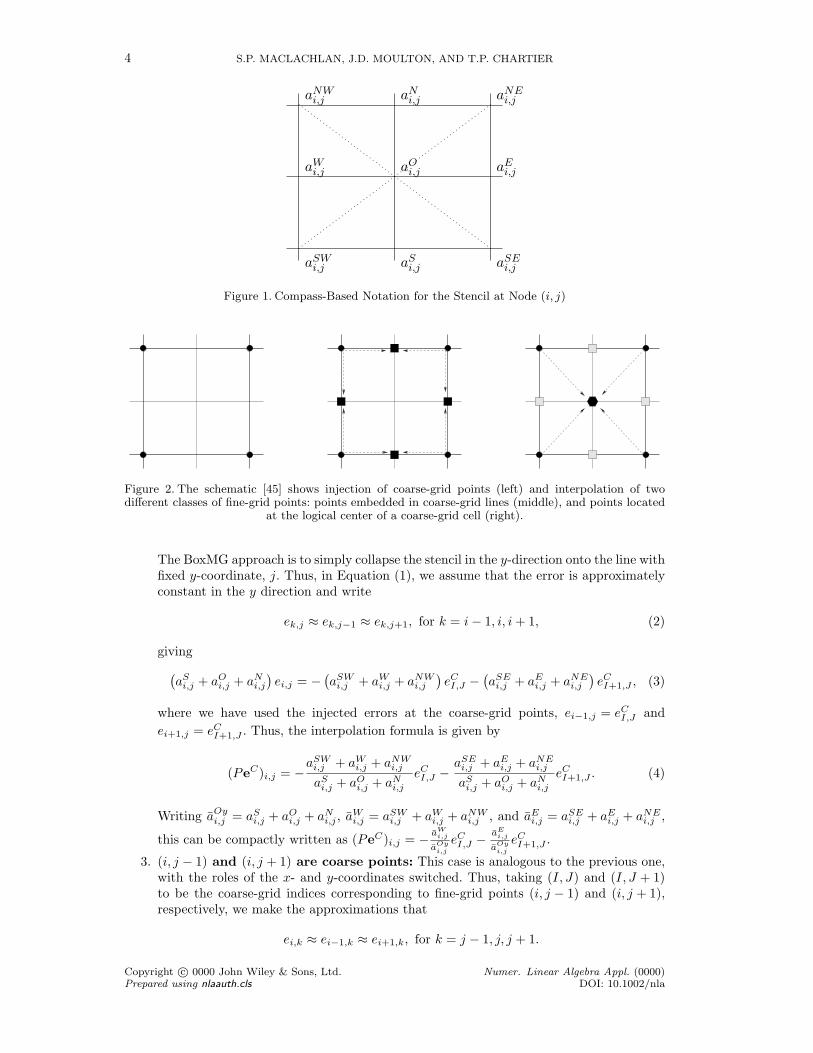
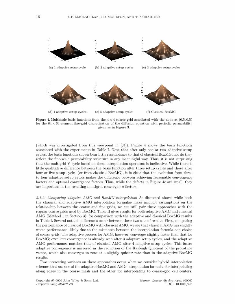
Figure 4. Multiscale basis functions from the 4× 4 coarse grid associated with the node at (0.5, 0.5)for the 64× 64 element fine-grid discretization of the diffusion equation with periodic permeability
given as in Figure 3.
(which was investigated from this viewpoint in [34]). Figure 4 shows the basis functionsassociated with the experiments in Table I. Note that after only one or two adaptive setupcycles, the basis functions shown bear little resemblance to that of classical BoxMG, nor do theyreflect the fine-scale permeability structure in any meaningful way. Thus, it is not surprisingthat the multigrid V-cycle based on these interpolation operators is ineffective. While there islittle qualitative difference between the basis function after three setup cycles and those afterfour or five setup cycles (or from classical BoxMG), it is clear that the evolution from threeto four adaptive setup cycles makes the difference between achieving reasonable convergencefactors and optimal convergence factors. Thus, while the defects in Figure 4c are small, theyare important in the resulting multigrid convergence factors.
4.1.2. Comparing adaptive AMG and BoxMG interpolation As discussed above, while boththe classical and adaptive AMG interpolation formulae make implicit assumptions on therelationship between the coarse and fine grids, we can still pair these approaches with theregular coarse grids used by BoxMG. Table II gives results for both adaptive AMG and classicalAMG (Method 1 in Section 3), for comparison with the adaptive and classical BoxMG resultsin Table I. Several notable differences occur between these two sets of results. First, comparingthe performance of classical BoxMG with classical AMG, we see that classical AMG has slightlyworse performance, likely due to the mismatch between the interpolation formula and choiceof coarse grids. The adaptive process for AMG, however, converges slightly faster than that forBoxMG; excellent convergence is already seen after 3 adaptive setup cycles, and the adaptiveAMG performance matches that of classical AMG after 4 adaptive setup cycles. This fasteradaptive convergence is mirrored in the reduction of the Rayleigh Quotient of the prototypevector, which also converges to zero at a slightly quicker rate than in the adaptive BoxMGresults.
Two interesting variants on these approaches occur when we consider hybrid interpolationschemes that use one of the adaptive BoxMG and AMG interpolation formulae for interpolatingalong edges in the coarse mesh and the other for interpolating to coarse-grid cell centers,
Copyright c© 0000 John Wiley & Sons, Ltd. Numer. Linear Algebra Appl. (0000)Prepared using nlaauth.cls DOI: 10.1002/nla
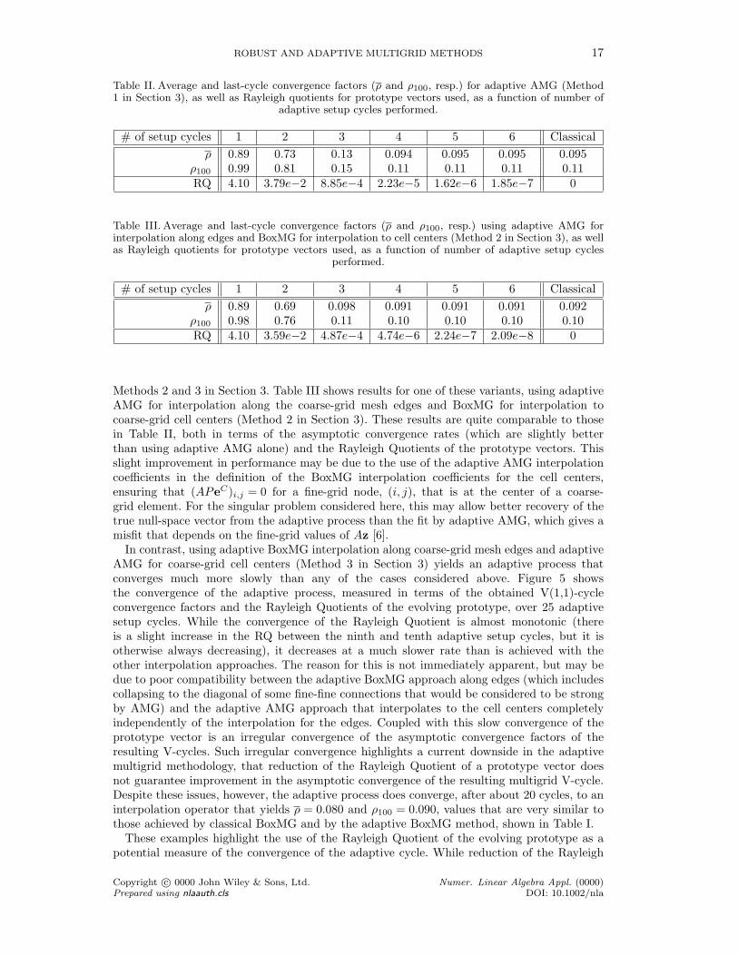
ROBUST AND ADAPTIVE MULTIGRID METHODS 17
Table II. Average and last-cycle convergence factors (ρ and ρ100, resp.) for adaptive AMG (Method1 in Section 3), as well as Rayleigh quotients for prototype vectors used, as a function of number of
adaptive setup cycles performed.
# of setup cycles 1 2 3 4 5 6 Classicalρ 0.89 0.73 0.13 0.094 0.095 0.095 0.095
ρ100 0.99 0.81 0.15 0.11 0.11 0.11 0.11RQ 4.10 3.79e−2 8.85e−4 2.23e−5 1.62e−6 1.85e−7 0
Table III. Average and last-cycle convergence factors (ρ and ρ100, resp.) using adaptive AMG forinterpolation along edges and BoxMG for interpolation to cell centers (Method 2 in Section 3), as wellas Rayleigh quotients for prototype vectors used, as a function of number of adaptive setup cycles
performed.
# of setup cycles 1 2 3 4 5 6 Classicalρ 0.89 0.69 0.098 0.091 0.091 0.091 0.092
ρ100 0.98 0.76 0.11 0.10 0.10 0.10 0.10RQ 4.10 3.59e−2 4.87e−4 4.74e−6 2.24e−7 2.09e−8 0
Methods 2 and 3 in Section 3. Table III shows results for one of these variants, using adaptiveAMG for interpolation along the coarse-grid mesh edges and BoxMG for interpolation tocoarse-grid cell centers (Method 2 in Section 3). These results are quite comparable to thosein Table II, both in terms of the asymptotic convergence rates (which are slightly betterthan using adaptive AMG alone) and the Rayleigh Quotients of the prototype vectors. Thisslight improvement in performance may be due to the use of the adaptive AMG interpolationcoefficients in the definition of the BoxMG interpolation coefficients for the cell centers,ensuring that (APeC)i,j = 0 for a fine-grid node, (i, j), that is at the center of a coarse-grid element. For the singular problem considered here, this may allow better recovery of thetrue null-space vector from the adaptive process than the fit by adaptive AMG, which gives amisfit that depends on the fine-grid values of Az [6].
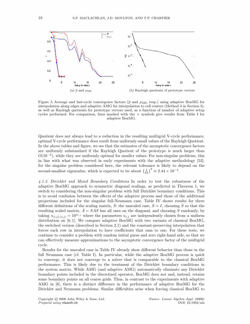
In contrast, using adaptive BoxMG interpolation along coarse-grid mesh edges and adaptiveAMG for coarse-grid cell centers (Method 3 in Section 3) yields an adaptive process thatconverges much more slowly than any of the cases considered above. Figure 5 showsthe convergence of the adaptive process, measured in terms of the obtained V(1,1)-cycleconvergence factors and the Rayleigh Quotients of the evolving prototype, over 25 adaptivesetup cycles. While the convergence of the Rayleigh Quotient is almost monotonic (thereis a slight increase in the RQ between the ninth and tenth adaptive setup cycles, but it isotherwise always decreasing), it decreases at a much slower rate than is achieved with theother interpolation approaches. The reason for this is not immediately apparent, but may bedue to poor compatibility between the adaptive BoxMG approach along edges (which includescollapsing to the diagonal of some fine-fine connections that would be considered to be strongby AMG) and the adaptive AMG approach that interpolates to the cell centers completelyindependently of the interpolation for the edges. Coupled with this slow convergence of theprototype vector is an irregular convergence of the asymptotic convergence factors of theresulting V-cycles. Such irregular convergence highlights a current downside in the adaptivemultigrid methodology, that reduction of the Rayleigh Quotient of a prototype vector doesnot guarantee improvement in the asymptotic convergence of the resulting multigrid V-cycle.Despite these issues, however, the adaptive process does converge, after about 20 cycles, to aninterpolation operator that yields ρ = 0.080 and ρ100 = 0.090, values that are very similar tothose achieved by classical BoxMG and by the adaptive BoxMG method, shown in Table I.
These examples highlight the use of the Rayleigh Quotient of the evolving prototype as apotential measure of the convergence of the adaptive cycle. While reduction of the Rayleigh
Copyright c© 0000 John Wiley & Sons, Ltd. Numer. Linear Algebra Appl. (0000)Prepared using nlaauth.cls DOI: 10.1002/nla
18 S.P. MACLACHLAN, J.D. MOULTON, AND T.P. CHARTIER
(a) ρ and ρ100 (b) Rayleigh quotients of prototype vectors
Figure 5. Average and last-cycle convergence factors (ρ and ρ100, resp.) using adaptive BoxMG forinterpolation along edges and adaptive AMG for interpolation to cell centers (Method 3 in Section 3),as well as Rayleigh quotients for prototype vectors used, as a function of number of adaptive setupcycles performed. For comparison, lines marked with the × symbols give results from Table I for
adaptive BoxMG.
Quotient does not always lead to a reduction in the resulting multigrid V-cycle performance,optimal V-cycle performance does result from uniformly small values of the Rayleigh Quotient.In the above tables and figure, we see that the estimates of the asymptotic convergence factorsare uniformly substandard if the Rayleigh Quotient of the prototype is much larger thanO(10−4), while they are uniformly optimal for smaller values. For non-singular problems, thisin line with what was observed in early experiments with the adaptive methodology [53];for the singular problem considered here, the relevant tolerance is likely to depend on thesecond-smallest eigenvalue, which is expected to be about
(164
)2 ≈ 2.44× 10⁻⁴.
4.1.3. Dirichlet and Mixed Boundary Conditions In order to test the robustness of theadaptive BoxMG approach to symmetric diagonal scalings, as predicted in Theorem 1, weswitch to considering the non-singular problem with full Dirichlet boundary conditions. Thisis to avoid confusion between the effects of the adaptive process and those of the additionalprojections included for the singular full-Neumann case. Table IV shows results for threedifferent definitions of the scaling matrix, S: the unscaled case, S = I, choosing S so that theresulting scaled matrix, A = SAS has all ones on the diagonal, and choosing S randomly, bytaking s(i,j),(i,j) = 10ui,j where the parameters ui,j are independently chosen from a uniformdistribution on [0, 1]. We compare adaptive BoxMG with two variants of classical BoxMG,the switched version (described in Section 2.1) and the constant-preserving interpolation thatforces each row in interpolation to have coefficients that sum to one. For these tests, wecontinue to consider a problem with random initial guess and zero right-hand side, so that wecan effectively measure approximations to the asymptotic convergence factor of the multigridcycle.
Results for the unscaled case in Table IV already show different behavior than those in thefull Neumann case (cf. Table I). In particular, while the adaptive BoxMG process is quickto converge, it does not converge to a solver that is comparable to the classical BoxMGperformance. This is likely due to the treatment of the Dirichlet boundary conditions inthe system matrix. While AMG (and adaptive AMG) automatically eliminate any Dirichletboundary points included in the discretized operator, BoxMG does not and, instead, retainssome boundary points on all coarse grids. Thus, in contrast to the experiments with adaptiveAMG in [6], there is a distinct difference in the performance of adaptive BoxMG for theDirichlet and Neumann problems. Similar difficulties arise when forcing classical BoxMG to
Copyright c© 0000 John Wiley & Sons, Ltd. Numer. Linear Algebra Appl. (0000)Prepared using nlaauth.cls DOI: 10.1002/nla
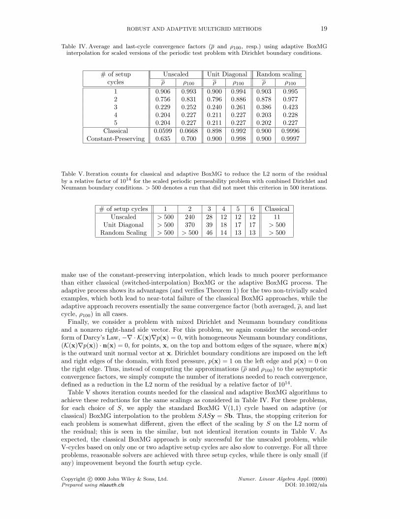
ROBUST AND ADAPTIVE MULTIGRID METHODS 19
Table IV. Average and last-cycle convergence factors (ρ and ρ100, resp.) using adaptive BoxMGinterpolation for scaled versions of the periodic test problem with Dirichlet boundary conditions.
# of setup Unscaled Unit Diagonal Random scalingcycles ρ ρ100 ρ ρ100 ρ ρ100
1 0.906 0.993 0.900 0.994 0.903 0.9952 0.756 0.831 0.796 0.886 0.878 0.9773 0.229 0.252 0.240 0.261 0.386 0.4234 0.204 0.227 0.211 0.227 0.203 0.2285 0.204 0.227 0.211 0.227 0.202 0.227
Classical 0.0599 0.0668 0.898 0.992 0.900 0.9996Constant-Preserving 0.635 0.700 0.900 0.998 0.900 0.9997
Table V. Iteration counts for classical and adaptive BoxMG to reduce the L2 norm of the residualby a relative factor of 1014 for the scaled periodic permeability problem with combined Dirichlet andNeumann boundary conditions. > 500 denotes a run that did not meet this criterion in 500 iterations.
# of setup cycles 1 2 3 4 5 6 ClassicalUnscaled > 500 240 28 12 12 12 11
Unit Diagonal > 500 370 39 18 17 17 > 500Random Scaling > 500 > 500 46 14 13 13 > 500
make use of the constant-preserving interpolation, which leads to much poorer performancethan either classical (switched-interpolation) BoxMG or the adaptive BoxMG process. Theadaptive process shows its advantages (and verifies Theorem 1) for the two non-trivially scaledexamples, which both lead to near-total failure of the classical BoxMG approaches, while theadaptive approach recovers essentially the same convergence factor (both averaged, ρ, and lastcycle, ρ100) in all cases.
Finally, we consider a problem with mixed Dirichlet and Neumann boundary conditionsand a nonzero right-hand side vector. For this problem, we again consider the second-orderform of Darcy’s Law, −∇ · K(x)∇p(x) = 0, with homogeneous Neumann boundary conditions,(K(x)∇p(x)) · n(x) = 0, for points, x, on the top and bottom edges of the square, where n(x)is the outward unit normal vector at x. Dirichlet boundary conditions are imposed on the leftand right edges of the domain, with fixed pressure, p(x) = 1 on the left edge and p(x) = 0 onthe right edge. Thus, instead of computing the approximations (ρ and ρ100) to the asymptoticconvergence factors, we simply compute the number of iterations needed to reach convergence,defined as a reduction in the L2 norm of the residual by a relative factor of 1014.
Table V shows iteration counts needed for the classical and adaptive BoxMG algorithms toachieve these reductions for the same scalings as considered in Table IV. For these problems,for each choice of S, we apply the standard BoxMG V(1,1) cycle based on adaptive (orclassical) BoxMG interpolation to the problem SASy = Sb. Thus, the stopping criterion foreach problem is somewhat different, given the effect of the scaling by S on the L2 norm ofthe residual; this is seen in the similar, but not identical iteration counts in Table V. Asexpected, the classical BoxMG approach is only successful for the unscaled problem, whileV-cycles based on only one or two adaptive setup cycles are also slow to converge. For all threeproblems, reasonable solvers are achieved with three setup cycles, while there is only small (ifany) improvement beyond the fourth setup cycle.
Copyright c© 0000 John Wiley & Sons, Ltd. Numer. Linear Algebra Appl. (0000)Prepared using nlaauth.cls DOI: 10.1002/nla
20 S.P. MACLACHLAN, J.D. MOULTON, AND T.P. CHARTIER
(a) Principle axis of 15 (b) Principle axis of 60
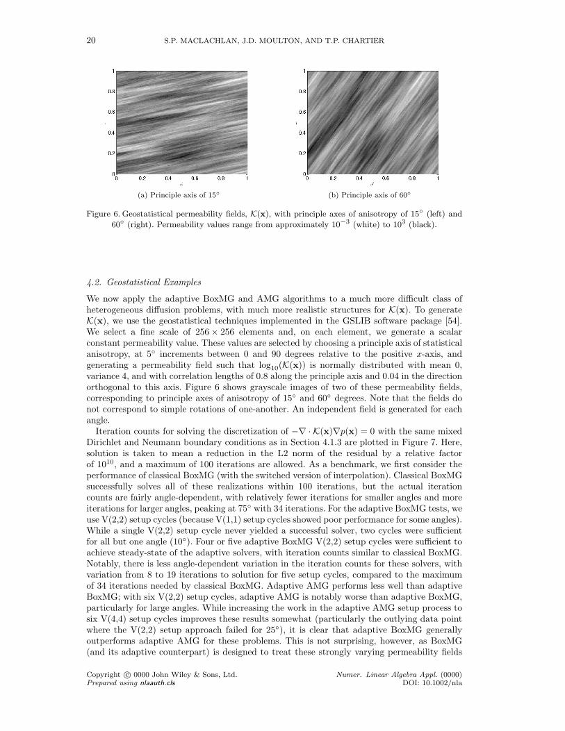
Figure 6. Geostatistical permeability fields, K(x), with principle axes of anisotropy of 15 (left) and
60 (right). Permeability values range from approximately 10−3 (white) to 103 (black).
4.2. Geostatistical Examples
We now apply the adaptive BoxMG and AMG algorithms to a much more difficult class ofheterogeneous diffusion problems, with much more realistic structures for K(x). To generateK(x), we use the geostatistical techniques implemented in the GSLIB software package [54].We select a fine scale of 256× 256 elements and, on each element, we generate a scalarconstant permeability value. These values are selected by choosing a principle axis of statisticalanisotropy, at 5 increments between 0 and 90 degrees relative to the positive x-axis, andgenerating a permeability field such that log10(K(x)) is normally distributed with mean 0,variance 4, and with correlation lengths of 0.8 along the principle axis and 0.04 in the directionorthogonal to this axis. Figure 6 shows grayscale images of two of these permeability fields,corresponding to principle axes of anisotropy of 15 and 60 degrees. Note that the fields donot correspond to simple rotations of one-another. An independent field is generated for eachangle.
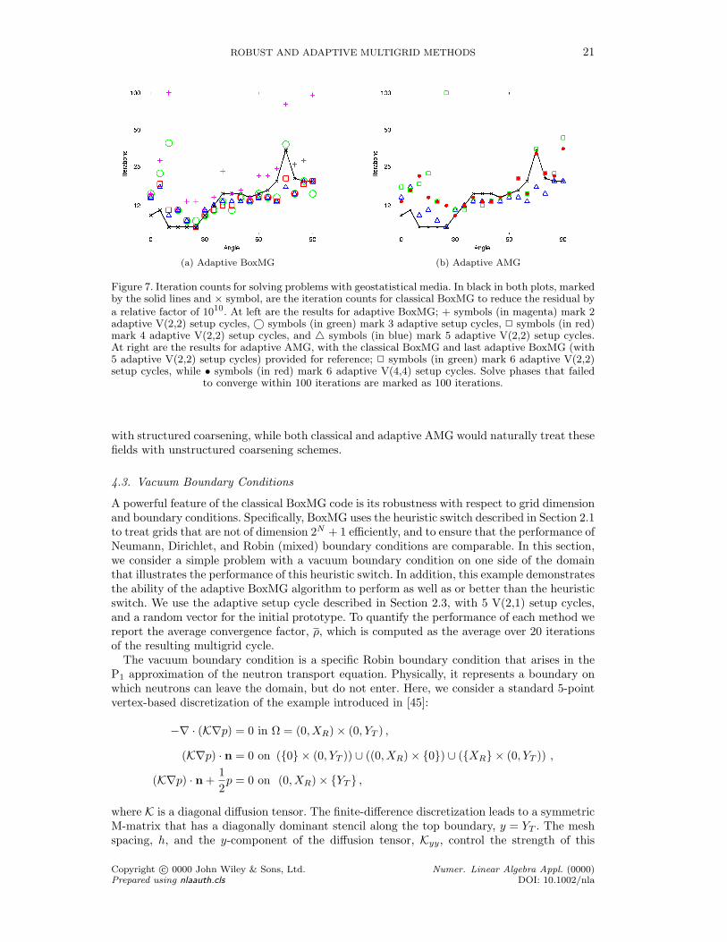
Iteration counts for solving the discretization of −∇ · K(x)∇p(x) = 0 with the same mixedDirichlet and Neumann boundary conditions as in Section 4.1.3 are plotted in Figure 7. Here,solution is taken to mean a reduction in the L2 norm of the residual by a relative factorof 1010, and a maximum of 100 iterations are allowed. As a benchmark, we first consider theperformance of classical BoxMG (with the switched version of interpolation). Classical BoxMGsuccessfully solves all of these realizations within 100 iterations, but the actual iterationcounts are fairly angle-dependent, with relatively fewer iterations for smaller angles and moreiterations for larger angles, peaking at 75 with 34 iterations. For the adaptive BoxMG tests, weuse V(2,2) setup cycles (because V(1,1) setup cycles showed poor performance for some angles).While a single V(2,2) setup cycle never yielded a successful solver, two cycles were sufficientfor all but one angle (10). Four or five adaptive BoxMG V(2,2) setup cycles were sufficient toachieve steady-state of the adaptive solvers, with iteration counts similar to classical BoxMG.Notably, there is less angle-dependent variation in the iteration counts for these solvers, withvariation from 8 to 19 iterations to solution for five setup cycles, compared to the maximumof 34 iterations needed by classical BoxMG. Adaptive AMG performs less well than adaptiveBoxMG; with six V(2,2) setup cycles, adaptive AMG is notably worse than adaptive BoxMG,particularly for large angles. While increasing the work in the adaptive AMG setup process tosix V(4,4) setup cycles improves these results somewhat (particularly the outlying data pointwhere the V(2,2) setup approach failed for 25), it is clear that adaptive BoxMG generallyoutperforms adaptive AMG for these problems. This is not surprising, however, as BoxMG(and its adaptive counterpart) is designed to treat these strongly varying permeability fields
Copyright c© 0000 John Wiley & Sons, Ltd. Numer. Linear Algebra Appl. (0000)Prepared using nlaauth.cls DOI: 10.1002/nla
ROBUST AND ADAPTIVE MULTIGRID METHODS 21
(a) Adaptive BoxMG (b) Adaptive AMG
Figure 7. Iteration counts for solving problems with geostatistical media. In black in both plots, markedby the solid lines and × symbol, are the iteration counts for classical BoxMG to reduce the residual bya relative factor of 1010. At left are the results for adaptive BoxMG; + symbols (in magenta) mark 2adaptive V(2,2) setup cycles, © symbols (in green) mark 3 adaptive setup cycles, 2 symbols (in red)mark 4 adaptive V(2,2) setup cycles, and 4 symbols (in blue) mark 5 adaptive V(2,2) setup cycles.At right are the results for adaptive AMG, with the classical BoxMG and last adaptive BoxMG (with5 adaptive V(2,2) setup cycles) provided for reference; 2 symbols (in green) mark 6 adaptive V(2,2)setup cycles, while • symbols (in red) mark 6 adaptive V(4,4) setup cycles. Solve phases that failed
to converge within 100 iterations are marked as 100 iterations.
with structured coarsening, while both classical and adaptive AMG would naturally treat thesefields with unstructured coarsening schemes.
4.3. Vacuum Boundary Conditions
A powerful feature of the classical BoxMG code is its robustness with respect to grid dimensionand boundary conditions. Specifically, BoxMG uses the heuristic switch described in Section 2.1to treat grids that are not of dimension 2N + 1 efficiently, and to ensure that the performance ofNeumann, Dirichlet, and Robin (mixed) boundary conditions are comparable. In this section,we consider a simple problem with a vacuum boundary condition on one side of the domainthat illustrates the performance of this heuristic switch. In addition, this example demonstratesthe ability of the adaptive BoxMG algorithm to perform as well as or better than the heuristicswitch. We use the adaptive setup cycle described in Section 2.3, with 5 V(2,1) setup cycles,and a random vector for the initial prototype. To quantify the performance of each method wereport the average convergence factor, ρ, which is computed as the average over 20 iterationsof the resulting multigrid cycle.
The vacuum boundary condition is a specific Robin boundary condition that arises in theP1 approximation of the neutron transport equation. Physically, it represents a boundary onwhich neutrons can leave the domain, but do not enter. Here, we consider a standard 5-pointvertex-based discretization of the example introduced in [45]:
−∇ · (K∇p) = 0 in Ω = (0, XR)× (0, YT ) ,
(K∇p) · n = 0 on (0 × (0, YT )) ∪ ((0, XR)× 0) ∪ (XR × (0, YT )) ,
(K∇p) · n +12p = 0 on (0, XR)× YT ,
where K is a diagonal diffusion tensor. The finite-difference discretization leads to a symmetricM-matrix that has a diagonally dominant stencil along the top boundary, y = YT . The meshspacing, h, and the y-component of the diffusion tensor, Kyy, control the strength of this
Copyright c© 0000 John Wiley & Sons, Ltd. Numer. Linear Algebra Appl. (0000)Prepared using nlaauth.cls DOI: 10.1002/nla
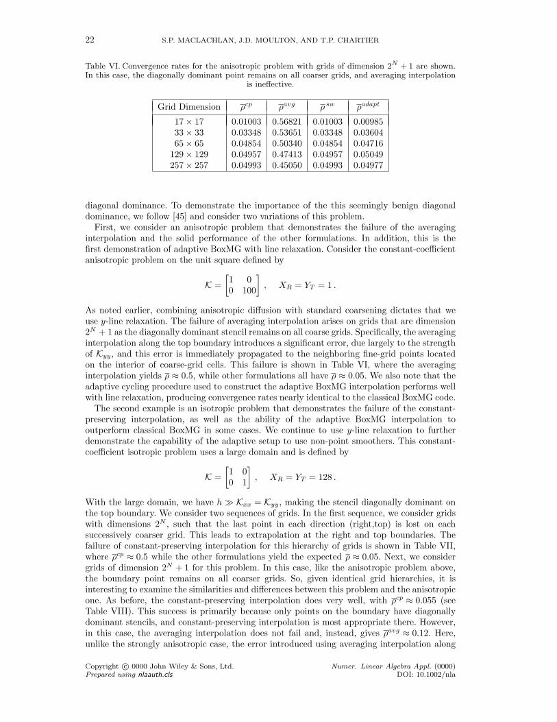
22 S.P. MACLACHLAN, J.D. MOULTON, AND T.P. CHARTIER
Table VI. Convergence rates for the anisotropic problem with grids of dimension 2N + 1 are shown.In this case, the diagonally dominant point remains on all coarser grids, and averaging interpolation
is ineffective.
Grid Dimension ρcp ρavg ρ sw ρadapt
17× 17 0.01003 0.56821 0.01003 0.0098533× 33 0.03348 0.53651 0.03348 0.0360465× 65 0.04854 0.50340 0.04854 0.04716
129× 129 0.04957 0.47413 0.04957 0.05049257× 257 0.04993 0.45050 0.04993 0.04977
diagonal dominance. To demonstrate the importance of the this seemingly benign diagonaldominance, we follow [45] and consider two variations of this problem.
First, we consider an anisotropic problem that demonstrates the failure of the averaginginterpolation and the solid performance of the other formulations. In addition, this is thefirst demonstration of adaptive BoxMG with line relaxation. Consider the constant-coefficientanisotropic problem on the unit square defined by
K =[1 00 100
], XR = YT = 1 .
As noted earlier, combining anisotropic diffusion with standard coarsening dictates that weuse y-line relaxation. The failure of averaging interpolation arises on grids that are dimension2N + 1 as the diagonally dominant stencil remains on all coarse grids. Specifically, the averaginginterpolation along the top boundary introduces a significant error, due largely to the strengthof Kyy, and this error is immediately propagated to the neighboring fine-grid points locatedon the interior of coarse-grid cells. This failure is shown in Table VI, where the averaginginterpolation yields ρ ≈ 0.5, while other formulations all have ρ ≈ 0.05. We also note that theadaptive cycling procedure used to construct the adaptive BoxMG interpolation performs wellwith line relaxation, producing convergence rates nearly identical to the classical BoxMG code.
The second example is an isotropic problem that demonstrates the failure of the constant-preserving interpolation, as well as the ability of the adaptive BoxMG interpolation tooutperform classical BoxMG in some cases. We continue to use y-line relaxation to furtherdemonstrate the capability of the adaptive setup to use non-point smoothers. This constant-coefficient isotropic problem uses a large domain and is defined by
K =[1 00 1
], XR = YT = 128 .
With the large domain, we have h Kxx = Kyy, making the stencil diagonally dominant onthe top boundary. We consider two sequences of grids. In the first sequence, we consider gridswith dimensions 2N , such that the last point in each direction (right,top) is lost on eachsuccessively coarser grid. This leads to extrapolation at the right and top boundaries. Thefailure of constant-preserving interpolation for this hierarchy of grids is shown in Table VII,where ρcp ≈ 0.5 while the other formulations yield the expected ρ ≈ 0.05. Next, we considergrids of dimension 2N + 1 for this problem. In this case, like the anisotropic problem above,the boundary point remains on all coarser grids. So, given identical grid hierarchies, it isinteresting to examine the similarities and differences between this problem and the anisotropicone. As before, the constant-preserving interpolation does very well, with ρcp ≈ 0.055 (seeTable VIII). This success is primarily because only points on the boundary have diagonallydominant stencils, and constant-preserving interpolation is most appropriate there. However,in this case, the averaging interpolation does not fail and, instead, gives ρavg ≈ 0.12. Here,unlike the strongly anisotropic case, the error introduced using averaging interpolation along
Copyright c© 0000 John Wiley & Sons, Ltd. Numer. Linear Algebra Appl. (0000)Prepared using nlaauth.cls DOI: 10.1002/nla
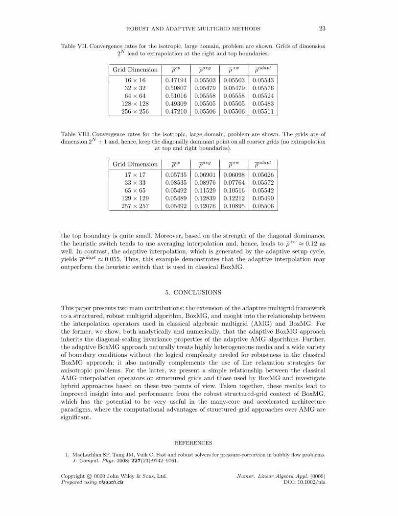
ROBUST AND ADAPTIVE MULTIGRID METHODS 23
Table VII. Convergence rates for the isotropic, large domain, problem are shown. Grids of dimension
2N lead to extrapolation at the right and top boundaries.
Grid Dimension ρcp ρavg ρ sw ρadapt
16× 16 0.47194 0.05503 0.05503 0.0554332× 32 0.50807 0.05479 0.05479 0.0557664× 64 0.51016 0.05558 0.05558 0.05524
128× 128 0.49309 0.05505 0.05505 0.05483256× 256 0.47210 0.05506 0.05506 0.05511
Table VIII. Convergence rates for the isotropic, large domain, problem are shown. The grids are of
dimension 2N + 1 and, hence, keep the diagonally dominant point on all coarser grids (no extrapolationat top and right boundaries).
Grid Dimension ρcp ρavg ρ sw ρadapt
17× 17 0.05735 0.06901 0.06098 0.0562633× 33 0.08535 0.08976 0.07764 0.0557265× 65 0.05492 0.11529 0.10516 0.05542
129× 129 0.05489 0.12839 0.12212 0.05490257× 257 0.05492 0.12076 0.10895 0.05506
the top boundary is quite small. Moreover, based on the strength of the diagonal dominance,the heuristic switch tends to use averaging interpolation and, hence, leads to ρ sw ≈ 0.12 aswell. In contrast, the adaptive interpolation, which is generated by the adaptive setup cycle,yields ρadapt ≈ 0.055. Thus, this example demonstrates that the adaptive interpolation mayoutperform the heuristic switch that is used in classical BoxMG.
5. CONCLUSIONS
This paper presents two main contributions: the extension of the adaptive multigrid frameworkto a structured, robust multigrid algorithm, BoxMG, and insight into the relationship betweenthe interpolation operators used in classical algebraic multigrid (AMG) and BoxMG. Forthe former, we show, both analytically and numerically, that the adaptive BoxMG approachinherits the diagonal-scaling invariance properties of the adaptive AMG algorithms. Further,the adaptive BoxMG approach naturally treats highly heterogeneous media and a wide varietyof boundary conditions without the logical complexity needed for robustness in the classicalBoxMG approach; it also naturally complements the use of line relaxation strategies foranisotropic problems. For the latter, we present a simple relationship between the classicalAMG interpolation operators on structured grids and those used by BoxMG and investigatehybrid approaches based on these two points of view. Taken together, these results lead toimproved insight into and performance from the robust structured-grid context of BoxMG,which has the potential to be very useful in the many-core and accelerated architectureparadigms, where the computational advantages of structured-grid approaches over AMG aresignificant.
REFERENCES
1. MacLachlan SP, Tang JM, Vuik C. Fast and robust solvers for pressure-correction in bubbly flow problems.J. Comput. Phys. 2008; 227(23):9742–9761.
Copyright c© 0000 John Wiley & Sons, Ltd. Numer. Linear Algebra Appl. (0000)Prepared using nlaauth.cls DOI: 10.1002/nla
24 S.P. MACLACHLAN, J.D. MOULTON, AND T.P. CHARTIER
2. Brandt A. Multi–level adaptive technique (MLAT) for fast numerical solution to boundary value problems.Proceedings of the Third International Conference on Numerical Methods in Fluid Mechanics, LectureNotes in Physics, vol. 18, Cabannes H, Teman R (eds.), Springer–Verlag: Berlin, 1973; 82–89.
3. Brandt A. Multi–level adaptive solutions to boundary–value problems. Math. Comp. 1977; 31:333–390.4. Brezina M, Falgout R, MacLachlan S, Manteuffel T, McCormick S, Ruge J. Adaptive smoothed aggregation
(αSA). SIAM J. Sci. Comput. 2004; 25(6):1896–1920.5. Brezina M, Falgout R, MacLachlan S, Manteuffel T, McCormick S, Ruge J. Adaptive smoothed aggregation
(αSA) multigrid. SIAM Rev. 2005; 47(2):317–346.6. Brezina M, Falgout R, MacLachlan S, Manteuffel T, McCormick S, Ruge J. Adaptive algebraic multigrid.
SIAM J. Sci. Comput. 2006; 27:1261–1286.7. Brandt A, Brannick J, Kahl K, Livshits I. Bootstrap AMG. SIAM Journal on Scientific Computing 2011;
33(2):612–632.8. H De Sterck, Manteuffel TA, McCormick SF, Nguyen Q, Ruge J. Multilevel adaptive aggregation for
Markov chains, with application to web ranking. SIAM J. Sci. Comput. 2008; 30(5):2235–2262.9. Borzı A. High-order discretization and multigrid solution of elliptic nonlinear constrained optimal control
problems. J. Comput. Appl. Math. 2007; 200(1):67–85.10. Borgers C, MacLachlan S. An angular multigrid method for monoenergetic particle beams in Flatland. J.
Comp. Phys. 2010; 229:2914–2931.11. Brezina M, Manteuffel T, McCormick S, Ruge J, Sanders G. Towards adaptive smoothed aggregation
(αSA) for nonsymmetric problems. SIAM J. Sci. Comput. 2010; 32:14–39.12. Haber E, MacLachlan S. A fast method for the solution of the Helmholtz equation. Journal of
Computational Physics 2011; 230(12):4403 – 4418.13. Ritter D, Sturmer M, Rude U. A fast-adaptive composite grid algorithm for solving the free-space Poisson
problem on the cell broadband engine. Numerical Linear Algebra with Applications 2010; 17(2-3):291–305.14. Bell N, Garland M. Implementing sparse matrix-vector multiplication on throughput-oriented processors.
SC ’09: Proceedings of the Conference on High Performance Computing Networking, Storage andAnalysis, ACM: New York, NY, USA, 2009; 1–11.
15. Minden V, Smith B, Knepley MG. Preliminary implementation of PETSc using GPUs. Proceedings ofthe 2010 International Workshop of GPU Solutions to Multiscale Problems in Science and Engineering,2010.
16. Alcouffe RE, Brandt A, Dendy JE, Painter JW. The multigrid method for the diffusion equation withstrongly discontinuous coefficients. SIAM J. Sci. Stat. Comput. 1981; 2:430–454.
17. Dendy JE. Black box multigrid. J. Comput. Phys. 1982; 48:366–386.18. Ruge JW, Stuben K. Algebraic multigrid (AMG). Multigrid Methods, Frontiers in Applied Mathematics,
vol. 3, McCormick SF (ed.). SIAM: Philadelphia, PA, 1987; 73–130.19. Brandt A, McCormick SF, Ruge JW. Algebraic multigrid (AMG) for automatic multigrid solution with
application to geodetic computations. Technical Report, Institute for Computational Studies, ColoradoState University 1982.
20. Brandt A, McCormick SF, Ruge JW. Algebraic multigrid (AMG) for sparse matrix equations. Sparsityand Its Applications, Evans DJ (ed.). Cambridge University Press: Cambridge, 1984.
21. Dendy JE. Black box multigrid for nonsymmetric problems. Appl. Math. Comput. 1983; 13:261–283.22. Dendy JE. Black box multigrid for systems. Appl. Math. Comput. 1986; 19:57–74.23. Dendy, Jr JE. Two multigrid methods for three-dimensional problems with discontinuous and anisotropic
coefficients. SIAM J. Sci. Statist. Comput. 1987; 8(5):673–685.24. Dendy JE. Black box multigrid for periodic and singular problems. Appl. Math. Comput. 1988; 25:1–10.25. Alber DM, Olson LN. Parallel coarse-grid selection. Numerical Linear Algebra with Applications 2007;
14(8):611–643.26. De Sterck H, Yang UM, Heys JJ. Reducing complexity in parallel algebraic multigrid preconditioners.
SIAM J. Matrix Anal. Appl. 2006; 27(4):1019–1039.27. De Sterck H, Falgout RD, Nolting JW, Yang UM. Distance-two interpolation for parallel algebraic
multigrid. Numer. Linear Algebra Appl. 2008; 15(2-3):115–139.28. Livne O. Coarsening by compatible relaxation. Numer. Linear Alg. Appl. 2004; 11(2):205–227.29. Brannick JJ, Falgout RD. Compatible relaxation and coarsening in algebraic multigrid. SIAM Journal on
Scientific Computing 2010; 32(3):1393–1416.30. MacLachlan S, Saad Y. A greedy strategy for coarse-grid selection. SIAM J. Sci. Comput. 2007;
29(5):1826–1853.31. Austin TM, Trew ML, Pullan AJ. Solving the cardiac bidomain equations for discontinuous conductivities.
IEEE Trans Biomed Eng July 2006; 53(7):1265–1272.32. Jiang Y, Pjesivac J, Cantrell C, Freyer J. A multiscale model for avascular tumor growth 2005. Preprint:
LA-UR-04-5498.33. Aruliah DA, Ascher UM. Multigrid preconditioning for Krylov methods for time-harmonic Maxwell’s
equations in three dimensions. SIAM Journal on Scientific Computing 2002; 24(2):702–718.34. MacLachlan SP, Moulton JD. Multilevel upscaling through variational coarsening. Water Resour. Res.
2006; 42.35. Moulton J, Knapek S, Dendy J. Multilevel upscaling in heterogeneous porous media. CNLS report, Center
for Nonlinear Studies, Los Alamos National Laboratory, Los Alamos, New Mexico 1999.36. Moulton JD, Dendy JE, Hyman JM. The black box multigrid numerical homogenization algorithm. J.
Comput. Phys. 1998; 141:1–29.37. Adams M, Brezina M, Hu J, Tuminaro R. Parallel multigrid smoothing: polynomial versus Gauss-Seidel.
J. Comput. Phys. 2003; 188:593–610.
Copyright c© 0000 John Wiley & Sons, Ltd. Numer. Linear Algebra Appl. (0000)Prepared using nlaauth.cls DOI: 10.1002/nla
ROBUST AND ADAPTIVE MULTIGRID METHODS 25
38. Brezina M, Tong C, Becker R. Parallel algebraic multigrids for structural mechanics. SIAM J. Sci. Comput.2006; 27(5):1534–1554.
39. Henson V, Yang U. BoomerAMG: a parallel algebraic multigrid solver and preconditioner. AppliedNumerical Mathematics 2002; 41:155–177.
40. Tuminaro RS, Tong C. Parallel smoothed aggregation multigrid: Aggregation strategies on massivelyparallel machines. SuperComputing 2000 Proceedings, Donnelley J (ed.), 2000.
41. Yang UM. Parallel algebraic multigrid methods—high performance preconditioners. Numerical solutionof partial differential equations on parallel computers, Lect. Notes Comput. Sci. Eng., vol. 51. Springer:Berlin, 2006; 209–236.
42. Brannick J, Brezina M, Keyes D, Livne O, Livshits I, MacLachlan S, Manteuffel T, McCormick S, Ruge J,Zikatanov L. Adaptive smoothed aggregation in lattice QCD. Domain Decomposition Methods in Scienceand Engineering XVI, Lecture Notes in Computational Science and Engineering, vol. 55. Springer, 2007;505–512.
43. Babich R, Brannick J, Brower RC, Clark MA, Manteuffel TA, McCormick SF, Osborn JC, Rebbi C.Adaptive multigrid algorithm for the lattice Wilson-Dirac operator. arXiv Jan 2010; hep-lat.
44. Brannick J, Brower RC, Clark MA, Osborn JC, Rebbi C. Adaptive multigrid algorithm for lattice QCD.Physical Review Letters 2008; 100(4):041601.
45. Dendy, Jr JE, Moulton JD. Black box multigrid with coarsening by a factor of three. Numerical LinearAlgebra with Applications 2010; 17(2-3):577–598.
46. P Vanek, Mandel J, Brezina M. Algebraic multigrid by smoothed aggregation for second and fourth orderelliptic problems. Computing 1996; 56:179–196.
47. Brannick J, Frommer A, Kahl K, MacLachlan S. Adaptive reduction-based multigrid for nearly singularand highly disordered physical systems. Electron. Trans. Numer. Anal. 2010; 37:276–295.
48. Chartier T, Orr D. Adaptive multigrid via subcycling on complementary grids 2007; In progress.49. MacLachlan S, Manteuffel T, McCormick S. Adaptive reduction-based AMG. Numer. Linear Alg. Appl.
2006; 13:599–620.50. Chow E. An aggregation multilevel method using smooth error vectors. SIAM J. Sci. Comput. 2006;
27:1727–1741.51. Briggs WL, Henson VE, McCormick SF. A Multigrid Tutorial. SIAM Books: Philadelphia, 2000. Second
edition.52. Grauschopf T, Griebel M, Regler H. Additive multilevel-preconditioners based on bilinear interpolation,
matrix dependent geometric coarsening and algebraic multigrid coarsening for second order elliptic PDEs.Appl. Numer. Math. 1997; 23:63–96.
53. MacLachlan S. Improving robustness in multiscale methods. PhD Thesis, Univerity of Colorado at Boulder,Boulder, Colorado 2004.
54. Deutsch C, Journel A. GSLIB, geostatistical software library and user’s guide. Second edn., OxfordUniversity Press: Oxford, 1998.
Copyright c© 0000 John Wiley & Sons, Ltd. Numer. Linear Algebra Appl. (0000)Prepared using nlaauth.cls DOI: 10.1002/nla


![ROBUST SOLUTION OF SINGULARLY PERTURBED PROBLEMS …niall/Research/MultiGrid_RD_300812.pdf · Robust solution of SPPs using multigrid methods 3 We shall assume that ε∈ (0,1] and](https://static.fdocuments.in/doc/165x107/5e9752b1f4f00c1b8905ec86/robust-solution-of-singularly-perturbed-problems-niallresearchmultigridrd300812pdf.jpg)