Robust Adaptive Coverage for Robotic Sensor...

Robust Adaptive Coverage for Robotic SensorNetworks

Mac Schwager, Michael P. Vitus, Daniela Rus, and Claire J. Tomlin

Abstract This paper presents a distributed control algorithm to drive a group ofrobots to spread out over an environment and provide adaptive sensor coverage ofthat environment. The robots use an on-line learning mechanism to approximatethe areas in the environment which require more concentrated sensor coverage,while simultaneously exploring the environment before moving to final positionsto provide this coverage. More precisely, the robots learn a scalar field, called theweighting function, representing the relative importance of different regions in theenvironment, and use a Traveling Salesperson based exploration method, followedby a Voronoi-based coverage controller to position themselves for sensing over theenvironment. The algorithm differs from previous approaches in that provable ro-bustness is emphasized in the representation of the weighting function. It is provedthat the robots approximate the weighting function with a known bounded error, andthat they converge to locations that are locally optimal for sensing with respect tothe approximate weighting function. Simulations using empirically measured lightintensity data are presented to illustrate the performance of the method.

Mac SchwagerGRASP Lab, University of Pennsylvania, 3330 Walnut St, PA 19104, USA, andComputer Science and Artificial Intelligence Lab, MIT, 77 Massachusetts Ave., Cambridge, MA,02139, USA, e-mail: [email protected]

Michael P. VitusAeronautics and Astronautics, Stanford University, Stanford, CA 94305, USA,e-mail: [email protected]

Daniela RusComputer Science and Artificial Intelligence Lab, MIT, 77 Massachusetts Ave., Cambridge, MA02139, USA, e-mail: [email protected]

Claire J. TomlinElectrical Engineering and Computer Sciences, UC Berkeley, Berkeley, CA 94708, USA,e-mail: [email protected]

1

2 Mac Schwager, Michael P. Vitus, Daniela Rus, and Claire J. Tomlin

1 IntroductionIn this paper we present a distributed control algorithm to command a group ofrobots to explore an unknown environment while providing adaptive sensor cov-erage of interesting areas within the environment. This algorithm has many appli-cations in controlling teams of robots to perform tasks such as search and rescuemissions, environmental monitoring, automatic surveillance of rooms, buildings, ortowns, or simulating collaborative predatory behavior. As an example application,Japan was hit by a major earthquake on March 11, 2011 that triggered a devastat-ing tsunami causing catastrophic damage to the nuclear reactors at Fukushima. Dueto the risk of radiation exposure, humans could not inspect (or repair) the nuclearreactors, however, a team of robots could be used to monitor the changing levelsof radiation. Using the proposed algorithm, the robots would concentrate on areaswhere the radiation was most dangerous, continually providing updated informationon how the radiation was evolving. This information could be used to notify peoplein eminent danger of radiation exposure due to the changing conditions. Similarly,consider a team of waterborne robots charged with cleaning up an oil spill. Ourcontroller allows the robots to distribute themselves over the spill, learn the areaswhere the spill is most severe and concentrate their efforts on those areas, withoutneglecting the areas where the spill is not as severe.

Sensor coverage algorithms have been receiving a great deal of attention in recentyears. Cortes et al. [Cortes et al., 2004] considered the problem of findin an optimalsensing configuration for a group of mobile robots. They used concepts from loca-tional optimization [Weber, 1929, Drezner, 1995] to control the robots based upongradient descent of a weighting function which encodes the sensing quality and cov-erage of the environment. This weighting function can be viewed as describing theimportance of areas in the environment. The control law for each robot is distributedand only depends on the robot’s position and the positions of its neighbors’. How-ever, all robots are required to know the weighting function a priori which restrictsthe algorithm from being deployed in unknown environments. There have been sev-eral extensions to this formulation of coverage control. In [Cortes et al., 2005], therobots were assumed to have a limited sensing or communication range. Pimenta etal. [Pimenta et al., 2008a] incorporated heterogeneous robots, and extended the al-gorithm to handle nonconvex environments. The work [Martınez, 2010] used a dis-tributed interpolation scheme to recursively estimate the weighting function. Sim-ilarly, [Schwager et al., 2009] removed the requirement of knowing the weightingfunction a priori by learning a basis function approximation of the weighting func-tion on-line. This strategy has provable convergence properties, but requires that theweighting function lies in a known set of functions. The purpose of the present workis to remove this restriction, greatly broadening the class of weighting functions thatcan be approximated.

Similar frameworks have been used for multi-robot problems in a stochastic set-ting [Arsie and Frazzoli, 2007]. There are also a number of other notions of multi-robot sensor coverage (e.g. [Choset, 2001, Latimer IV et al., 2002] and [Butler andRus, 2004, Ogren et al., 2004]), but we choose to adopt the locational optimizationapproach for its interesting possibilities for analysis and its compatibility with exist-

Robust Adaptive Coverage for Robotic Sensor Networks 3

ing ideas in adaptive control [Narendra and Annaswamy, 1989, Sastry and Bodson,1989, Slotine and Li, 1991].

As noted above, this work extends [Schwager et al., 2009] by removing restric-tions on the weighting function, so that a much broader class of weighting functionscan be provably approximated. Typically, the form of the weighting function is notknown a priori, and if this is not accounted for directly then the learning algorithmcould chatter between models or even become unstable. Also, in simulations per-formed with a realistic weighting function, the original algorithm only explores ina local neighborhood of the robots resulting in a poor approximation of the weight-ing function. However, the algorithm we propose here explores the entire space,successfully learning the weighting function with provable robustness. The robotsfirst partition the environment and perform a Traveling Sales Person (TSP) baseddistributed exploration, so that the unknown weighting function can be adequatelyapproximated. They then switch, in an asynchronous and distributed fashion, to acoverage mode in which they deploy over the environment to achieve positions thatare advantageous for sensing. The robots use an on-line learning mechanism to ap-proximate the weighting function. Since we do not assume the robots can perfectlyapproximate the weighting function, the parameter adaptation law for learning thisfunction must be carefully constructed to be robust to function approximation errors.

Without specifically designing for such robustness, it is known that many differ-ent types of instability [Ioannou and Kokotovic, 1984] can occur. Several techniqueshave been proposed in the adaptive control literature to handle this kind of robust-ness, including using a dead-zone [Peterson and Narendra, 1982,Samson, 1983], theσ -modification [Ioannou and Kokotovic, 1984], and the e1- modification [Naren-dra and Annaswamy, 1987]. We chose to adapt a dead-zone technique, and provethat the robots learn a function that has bounded difference from the true function,while converging to positions that are locally optimal for sensing with respect to thelearned function.

The paper is organized as follows. In Section 2 we introduce notation and for-mulate the problem. In Section 3 we describe the function approximation strategyand the control algorithm, and we prove the main convergence result of the paper.Section 4 gives the results of a numerical simulation with a weighting function thatwas determined from empirical measurements of light intensity in a room. Finally,conclusions and future work are discussed in Section 5.

2 Problem FormulationIn this section we build a model of the multi-robot system, the environment, andthe weighting function defining areas of importance in the environment. We thenformulate the robust adaptive coverage problem with respect to this model.

Let there be n robots with positions pi(t) in a planar environment Q ⊂ R2. Theenvironment is assumed to be compact and convex.1 We call the tuple of all robotpositions P = (p1, . . . , pn) ∈Qn the configuration of the multi-robot system, and we

1 These assumptions can be relaxed to certain classes of nonconvex environments with obstacles[Breitenmoser et al., 2010, Pimenta et al., 2008a, Caicedo and Zefran, 2008].


assume that the robots move with integrator dynamics

pi = ui, (1)

so that we can control their velocities directly through the control input ui. We definethe Voronoi partition of the environment to be V (P) = V1(P), . . . ,Vn(P), where

Vi(P) = q ∈ Q | ‖q− pi‖ ≤ ‖q− p j‖,∀ j 6= i,

and ‖ · ‖ is the `2-norm. We think of each robot i as being responsible for sensingin its associated Voronoi cell Vi. Next we define the communication network as anundirected graph in which all robots whose Voronoi cells touch share an edge inthe graph. This graph is known as the Delaunay graph. Then the set of neighbors ofrobot i is defined as Ni := j |Vi∪Vj 6= /0.

We now define a weighting function over the environment φ : Q 7→ R>0 (whereR>0 denotes the strictly positive real numbers). This weighting function is notknown by the robots. Intuitively, we want a high density of robots in areas whereφ(q) is large and a lower density where it is small. Finally, suppose that the robotshave sensors with which they can measure the value of the weighting function attheir own position, φ(pi) with very high precision, but that their quality of sensingat arbitrary points, φ(q), degrades quadratically in the distance between q and pi.That is to say the cost of a robot at pi sensing a point at q is given by 1

2‖q− pi‖2.Since each robot is responsible for sensing in its own Voronoi cell, the cost of allrobots sensing over all points in the environment is given by

H (P) =n

∑i=1

∫Vi(P)

12‖q− pi‖2

φ(q)dq. (2)

This is the overall objective function that we would like to minimize by controllingthe configuration of the multi-robot system.2

The gradient of H can be shown3 to be given by

∂H

∂ pi=−

∫Vi(P)

(q− pi)φ(q)dq =−Mi(P)(Ci(P)− pi), (3)

where we define Mi(P) :=∫

Vi(P) φ(q)dq and Ci(P) := 1/Mi(P)∫

Vi(P) qφ(q)dq. Wecall Mi the mass of the Voronoi cell i and Ci its centroid, and for efficiency of no-tation we will henceforth write these without the dependence on P. We would liketo control the robots to move to their Voronoi centroids, pi = Ci for all i, since from(3), this is a critical point of H , and if we reach such a configuration using gradientdescent, we know it will be a local minimum. Global optimization of H is knownto be NP-hard, hence it is standard in the literature to only consider local optimality.

2 We have pursued an intuitive development of this cost function, though more rigorous argumentscan also be made [Schwager et al., 2011]. This function is known in several fields of study includingthe placement of retail facilities [Drezner, 1995] and data compression [Lloyd, 1982].3 The computation of this gradient is more complex than it may seem, because the Voronoi cellsVi(P) depend on P, which results in extra integral terms. Fortunately, these extra terms all sum tozero, as shown in, e.g. [Pimenta et al., 2008b].


2.1 Approximate Weighting Function

Note that the cost function (2) and its gradient (3) rely on the weighting functionφ(q), which is not known to the robots. In this paper we provide a means by whichthe robots can approximate φ(q) online in a distributed way and move to decrease(2) with respect to this approximate φ(q).

To be more precise, each robot maintains a separate approximation of the weight-ing function, which we denote φ(q, t). These approximate weighting functionsare generated from a linear combination of m static basis functions, K (q) =[K1(q) · · ·Km(q)]T, where each basis function is a radially symmetric Gaussian ofthe form

K j(q) =1

2πσexp

−‖q−µ j‖2

2σ2

, (4)

with fixed width σ and fixed center µ j. Furthermore, the centers are arranged ina regular grid over Q. Each robot then forms its approximate weighting functionas a weighted sum of these basis functions φi(q, t) = K (q)Tai(t), where ai(t)is the parameter vector of robot i. Each element in the parameter vector is con-strained to lie within some lower and upper bounds 0 < amin < amax < ∞ so thatai(t) ∈ [amin,amax]m. This function approximation scheme is illustrated in Fig. 1.Robot i’s approximation of its Voronoi cell mass and centroid can then be defined as

Fig. 1 The weighting function approximation is illustrated in this simplified 2-D schematic. Thetrue weighting function φ(q) is approximated by robot i to be φi(q, t). The basis function vectorK (q) is shown as three Gaussians (dashed curves), and the parameter vector ai(t) denotes theweighting of each Gaussian.

Mi(P, t) :=∫

Vi(P) φi(q, t)dq and Ci(P, t) := 1/Mi(P, t)∫

Vi(P) qφi(q, t)dq, respectively.Again, we will drop the dependence of Mi and Ci on (P, t) for notational simplicity.

We measure the difference between an approximate weighting function and thetrue weighting function as the L∞ function norm of their difference, so that the bestapproximation is given by

a := argmina∈[amin,amax]m

maxq∈Q

|K (q)Ta−φ(q)|, (5)

and the optimal function approximation error is given by

φε(q) := K (q)Ta−φ(q). (6)

It will be shown in the proof of Theorem 1 that the L∞ norm gives the tightest ap-proximation bound with our proof technique. The only restriction that we put on


φ(q) is that it is bounded over the environment, or equivalently, the approximationerror is bounded, |φε(q)| ≤ φεmax < ∞. We assume that the robots have knowledgeof this bound, φεmax . The theoretical analysis in the previous work [Schwager et al.,2009] was not robust to function approximation errors in that it required φε(q)≡ 0.One of the main contributions here is to formulate an algorithm that is provably ro-bust to function approximation errors. We only require that the robots have a knownbound for the function approximation error, φεmax .

Finally, we define the parameter error as ai(t) := ai(t)− a. In what follows wedescribe an online tuning law by which robot i can tune its parameters, ai, to ap-proach a neighborhood of the optimal parameters, a. Our proposed controller thencauses the robots to converge to their approximate centroids, pi → Ci for all i. Anoverview of the geometrical objects involved in our set-up is shown in Figure 2.

: Weighting function: Convex environment

: Robot location

: Voronoi regionof robot

: True centroid

: Estimated centroid

True position error Estimatedposition error

Fig. 2 A graphical overview of the quantities involved in the controller is shown. The robots moveto cover a bounded, convex environment Q their positions are pi, and they each have a Voronoiregion Vi with a true centroid Ci and an estimated centroid Ci. The true centroid is determinedusing a sensory function φ(q), which indicates the relative importance of points q in Q. The robotsdo not know φ(q), so they calculate an estimated centroid using an approximation φi(q) learnedfrom sensor measurements of φ(q).

3 Robust Adaptive Coverage AlgorithmIn this section we describe the algorithm that drives the robots to spread out overthe environment while simultaneously approximating the weighting function online.The algorithm naturally decomposes into two parts: (1) the parameter adaptationlaw, by which each robot updates its approximate weighting function, and (2) thecontrol algorithm, which drives the robots to explore the environment before movingto their final positions for coverage. We describe these two parts in separate sectionsand then prove performance guarantees for the two working together.

3.1 Online Function Approximation

The parameters ai used to calculate φi(q, t) are adjusted according to a set of adap-tation laws which are introduced below. First, we define two quantities,


Λi(t) = Λ0 +∫

s∈Ωi(t)K (s)K (s)T ds, and λi(t) =

∫s∈Ωi(t)

K (s)φ(s)ds, (7)

where Ωi(t) = s | s = pi(τ) for someτ ∈ [0, t] is the set of points in the trajectoryof pi from time 0 to time t, and Λ0 is a positive definite matrix. The quantities in(7) can be calculated differentially by robot i using Λi(t) = Ki(t)Ki(t)T|pi(t)| withinitial condition Λ0, and λi(t) = Ki(t)φi(t)|pi(t)| with zero initial conditions, wherewe introduced the shorthand notation Ki(t) := K (pi(t)) and φi(t) := φ(pi(t)). Werequire that Λ0 > 0, though it can be arbitrarily small. This will ensure that Λi(t) > 0for all time because

∫s∈Ωi(t) K (s)K (s)T ds ≥ 0 and the sum of a positive semi-

definite matrix and a positive definite matrix is positive definite. This, in turn, en-sures that Λ

−1/2i always exists, which will be crucial in the control law and proof of

convergence below. As previously stated, robot i can measure φi(t) with its sensors.Now we define another quantity

Fi =

∫Vi

K (q)(q− pi)T dq∫

Vi(q− pi)K (q)T dq∫

Viφi(q)dq

. (8)

Notice that Fi can also be computed by robot i as it does not require any knowledgeof the true weighting function, φ .

The “pre” adaptation law for ai is now defined as

˙aprei =−γBdz(Λiai−λi)−ζ ∑

j∈Ni

li j(ai− a j)− kFiai. (9)

where γ , ζ , and k are positive gains, li j is the length of the shared Voronoi edgebetween robots i and j, and Bdz(·) is a dead zone function which gives a zero if itsargument is below some value. We will give Bdz careful attention in what followsas it is the main tool to ensure robustness to function approximation errors. Beforedescribing the dead zone in detail, we note that the three terms in (9) have an intu-itive interpretation. The first term is an integral of the function approximation errorover the robot’s trajectory, so that the parameter ai is tuned to decrease this error.The second term is the difference between the robot’s parameters and its neighbors’parameters. This term will be shown to lead to parameter consensus; the parametervectors for all robots will approach a common vector. The third term compensatesfor uncertainty in the centroid position estimate, and will be shown to ensure con-vergence of the robots to their estimated centroids. A more in-depth explanation ofeach of these terms can be found in [Schwager et al., 2009].

Finally, we give the parameter adaptation law by restricting the “pre” adaptationlaw so that the parameters remain within their prescribed limits [amin,amax] using aprojection operator. We introduce a matrix Iproji defined element-wise as

Iproji :=

0 for amin < ai( j) < amax0 for ai( j) = amin and ˙apre

i ( j)≥ 00 for ai( j) = amax and ˙apre

i ( j)≤ 01 otherwise,

(10)


where ( j) denotes the jth element for a vector and the jth diagonal element for amatrix. The entries of Iproji are only nonzero if the parameter is about to exceed itsbound. Now the parameters are changed according to the adaptation law

˙ai = Γ ( ˙aprei − Iproji˙aprei), (11)

where Γ ∈ Rm×m is a diagonal, positive definite gain matrix. Although the adapta-tion law given by (11) and (9) is notationally complicated, it has a straightforwardinterpretation, it is of low computational complexity, and it is composed entirely ofquantities that can be computed by robot i.

As mentioned above, the key innovation in this adaptation law compared with theone in [Schwager et al., 2009] is the dead zone function Bdz. We design this functionso that the parameters are only changed in response to function errors that could bereduced with different parameters. More specifically, the minimal function error thatcan be achieved is φε , as shown in (6). Therefore if the integrated parameter error(Λiai − λi) is less than φε integrated over the robot’s path, we have no reason tochange the parameters. We will show that the correct form for the dead zone toprevent unnecessary parameter adaptation is

Bdz(x) =

0 if C(x) < 0

x‖x‖

C(x) otherwise, (12)

where C(x) := ‖Λ1/2i ‖

(‖Λ

−1/2i x‖−‖Λ

−1/2i βi‖φεmax −‖Λ

−1/2i Λ0‖amax

)and

βi :=∫

s∈Ωi(t) K (s)ds. This condition can be evaluated by robot i since βi(t) canbe computed differentially from βi = Ki|pi| with zero initial conditions, we havealready seen how to compute Λi, and φεmax , amax, and Λ0 are known.

3.2 Control Algorithm

We propose to use a control algorithm that is composed of a set of control modes,with switching conditions to determine when the robots change from one mode tothe next. The robots first move to partition the basis function centers among oneanother, so that each center is assigned to one robot, then each robot executes aTraveling Salesperson (TSP) tour through all of the basis function centers that havebeen assigned to it. This tour will provide sufficient information so that the weight-ing function can be estimated well over all of the environment. Then the robotscarry out a centroidal Voronoi controller using the estimated weighting function todrive to final positions. We call the first mode the “partitioning” mode, the secondthe “exploration” mode, and the third the “coverage” mode. This sequence of con-trol modes is executed asynchronously in a distributed fashion, during which thefunction approximation parameters are updated continually with (11) and (9).

For each robot we define a mode variable Mii ∈ partition,explore,cover. Inorder to coordinate their mode switches, each robot also maintains an estimate ofthe modes of all the other robots, so that Mi j is the estimate by robot i of robotj’s mode, and Mi := (Mi1, . . . ,Min) is an n-tuple of robot i’s estimates of all


robots’ modes. Furthermore, the modes are ordered with respect to one another bypartition < explore < cover, so that the max(Mi,M j) function is the maximum be-tween each element of the two mode estimate tuples, Mi and M j, according to thisordering. These mode estimates are updated using the flooding communication pro-tocol described below. We first describe the algorithmic structure of the controller,then define the behavior within each mode, and finally prove the convergence of thecoupled control algorithm and learning algorithm to a desirable final configuration.

The two algorithms below run concurrently in different threads. Algorithm 1defines the switching conditions between control modes, and Algorithm 2 describesthe flooding protocol that each robot uses to maintain its mode estimates.

Algorithm 1 Switching Control Algorithm (executed by robot i)Require: Communication with Voronoi neighbors.Require: Knowledge of position, pi, in global coordinate frame.Require: Knowledge of the total number of robots n.Require: Knowledge of flooding algorithm (Algorithm 2) update period, T .Require: Access to mode estimates Mi updated from Algorithm 2.

while Mi 6= (explore, . . . ,explore) doif Mii == explore then

ui = [0, 0]T

elseui = upartition

iend ifif Distance to mean of basis function centers < εpartition and Mii == partition then

Mii = exploreend if

end whileCompute TSP tour through basis function centers N µ

iWait for nT seconds with ui = [0, 0]T

Execute TSP tourMii = coverwhile Mii == cover do

ui = ucoveri

end while

Algorithm 2 Mode Estimate Flooding (executed by robot i)Require: The network is connected.Require: The robots have synchronized clocks with which they broadcast during a pre-assigned

time slot.Initialize Mi = (partition, . . . ,partition)while 1 do

if Broadcast received from robot j thenMi = max(Mi,M j) (where partition < explore < cover)

end ifif Robot i’s turn to broadcast then

Broadcast Miend if

end while


The control laws within each mode are then defined as follows. In the partitionmode, each robot uses the controller

upartitioni = k

( 1|N µ

i | ∑j∈N

µ

i

µ j − pi

), (13)

where N µ

i := µ j | ‖µ j − pi‖ ≤ ‖µ j − pk‖∀k 6= i is the set of the closest basisfunction centers to robot i, µ j are the basis function centers from (4), and |N µ

i |is the number of elements in N µ

i . In the explore mode, each robot drives a tourthrough each basis function center in its neighborhood, µ j for j ∈ N µ

i . Any tourwill do, but a good choice is to use an approximate TSP tour. Finally, for the “cover”mode, each robot moves toward the centroid of its Voronoi cell using

ucoveri = k(Ci− pi), (14)

where k is the same positive gain from (9).Using the above control and function approximation algorithm, we can prove that

all robots converge to the estimated centroid of their Voronoi cells, that all robotsfunction approximation parameters converge to the same parameter vector, and thatthis parameter vector has a bounded error with the optimal parameter vector. This isstated formally in the following theorem.

Theorem 1 (Convergence). A network of robots with dynamics (1) using Algo-rithm 1 for control, Algorithm 2 for communication, and (9) and (11) for onlinefunction approximation has the following convergence guarantees:

limt→∞

‖pi(t)−Ci(P, t)‖= 0 ∀i, (15)

limt→∞

‖ai(t)− a j(t)‖= 0 ∀i, j, (16)

and limt→∞

‖ai(t)−a‖ ≤

∑nj=1 2‖Λ j(t)1/2‖

(‖Λ j(t)−1/2β j(t)‖φεmax +‖Λ j(t)−1/2Λ0‖amax

)mineig(∑n

j=1 Λ j(t))∀i.

(17)

Proof. The proof has two parts. The first part is to show that all robots reach “cover”mode and stay in “cover” mode. The second part uses a Lyapunov type proof tech-nique similar to the one in [Schwager et al., 2009] to show that once all robots arein “cover” mode, the convergence claims of (15), (16), and (17) follow.

Firstly, the “partition” mode simply implements a K-means clustering algorithm[Duda et al., 2001], in which the basis function centers are the points to be clustered,and the robots move to the cluster means. This algorithm is well-known to convergein the sense that for any εpartition there exists a time T partition

i at which the distancebetween the robot and the centers’ mean is less than εpartition, therefore all robotswill reach Mii = explore at some finite time. After this time, according to Algo-


rithm 1, a robot will remain stopped until all of its mode estimates have switchedto “explore.” Suppose the first robot to achieve Mi = (explore, . . . ,explore) doesso at time Tf . This means that at some time in the past all the other robots, j,have switched to M j j = explore and stopped moving, but none of them haveM j = (explore, . . . ,explore) (otherwise they would be the first). Therefore at Tf allrobots are stopped. Suppose the last robot to achieve Mi = (explore, . . . ,explore)does so at Tl . From the properties of Algorithm 2 we know that Tl − Tf ≤ nT(the maximum time between the first robot to obtain Mi = (explore, . . . ,explore)and the last robot to do so is nT ). At time Tl , the first robot to have Mi =(explore, . . . ,explore) will still be stopped, because it waits for nT seconds af-ter achieving Mi = (explore, . . . ,explore), hence when any robot obtains Mi =(explore, . . . ,explore), all other robots are stopped. Even though the robots maycompute their TSP tours at different times, they are all at the same positions whenthey do so. Therefore, each basis function center is in at least one robot’s TSP tour.Consequently, when all robots have completed their TSP tours, mineig

(∑

ni=1 Λi

)will be similar in size to maxeig

(∑

ni=1 Λi

), making the bound in (17) small.

Each tour is finite length, so it will terminate in finite time, hence each robot willeventually enter the “cover” mode. Furthermore, when some robots are in “cover”mode, and some are still in “explore” mode, the robots in “cover” mode will remaininside the environment Q. This is because Q is convex, and since Ci ∈ Vi ⊂ Q andpi ∈ Q, by convexity, the segment connecting the two is in Q. Since the robots haveintegrator dynamics (1), they will stay within the union of these segments over time,pi(t) ∈ ∪τ>0(Ci(τ)− pi(τ)), and therefore remain in the environment Q. Thus atsome finite time, T cover, all robots reach “cover” mode and are at positions inside Q.

Now, define a Lyapunov-like function

V = H +12 ∑

iaT

i Γ−1ai, (18)

which incorporates the sensing cost H , and is quadratic in the parameter errors ai.We will use Barbalat’s lemma to prove that V → 0 and then show that the claimsof the theorem follow. Barbalat’s lemma requires that V is lower bounded, non-increasing, and uniformly continuous. V is bounded below by zero since H isa sum of integrals of strictly positive functions, and the quadratic parameter errorterms are each bounded below by zero.

Now we will show that V ≤ 0. Taking the time derivative of V along the trajec-tories of the system and simplifying with (3) gives

V = ∑i

(−‖Ci− pi‖2kMi + aT

i kFiai + aTi Γ

−1 ˙ai).

Substituting for ˙ai with (11) and (9) gives

V =−∑i

(‖Ci− pi‖2kMi +γ aT

i Bdz(Λiai +λεi)+ζ aTi ∑

j∈Ni

li j(ai− a j)+ aTi Iproji

˙aprei

),


where λεi :=∫

s∈Ωi(t) K (s)φε(s)ds+Λ0a. Rearranging terms we get

V =−∑i

(‖Ci− pi‖2kMi + γ aT

i Bdz(Λiai +λεi)+ aTi Iproji

˙aprei

)−ζ

m

∑j=1

αTj L(P)α j,

(19)where α j := [a1 j · · · am j]T is the jth element in every robot’s parameter vector,stacked into a vector, and L(P) ≥ 0 is the graph Laplacian for the Delaunay graphwhich defines the robots communication network (please refer to the proof of The-orem 2 in [Schwager et al., 2009] for details). The first term inside the first sum isthe square of a norm, and therefore is non-negative. The third term in the first sumis non-negative by design (please see the proof of Theorem 1 from [Schwager et al.,2009] for details). The second sum is nonnegative because L(P)≥ 0. Therefore, theterm with the dead-zone operator Bdz is the only term in question, and this distin-guishes the Lyapunov construction here from the one in the proof of Theorem 1in [Schwager et al., 2009].

We now show that the dead-zone term is also non-negative by design. Supposethe condition C(Λiai +λεi) < 0 from (12). Then Bdz(Λ ai +λεi) = 0 and the term iszero. Now suppose C(Λiai +λεi)≥ 0. In that case we have

0≤ ‖Λ1/2i ‖

(‖Λ

−1/2i (Λiai +λεi)‖−‖Λ


−1/2i Λ0‖amax

),

which implies

0 ≤ ‖Λ−1/2i (Λiai +λεi)‖−‖Λ


−1/2i Λ0‖amax

≤ ‖Λ1/2i ai +Λ

−1/2λεi‖−

∥∥∥Λ−1/2i

(∫Ωi(t)

K (s)φε(s)ds+Λ0a)∥∥∥

≤ ‖Λ1/2i ai +Λ

−1/2i λεi‖

2− (Λ−1/2i λεi)

T(Λ 1/2i ai−Λ

−1/2i λεi)

= (Λ 1/2i ai)T(Λ 1/2

i ai +Λ−1/2i λεi)

= aTi (Λiai +λεi). (20)

Then from the definition of the dead-zone operator, Bdz(·), we have

aTBdz(Λiai +λεi) =aT(Λiai +λεi)‖Λiai +λεi‖

C(Λiai +λεi)≥ 0,

since the numerator was shown to be non-negative in (20), and C(·) is non-negativeby supposition. Therefore the dead-zone term is non-negative in this case as well.We conclude therefore that V ≤ 0.

The final condition to prove that V → 0 is that V must be uniformly continuous,which is a technical condition that was shown in [Schwager et al., 2009], Lemmas1 and 2. These lemmas also apply to our case, since our function V is the same asin that case except for the dead-zone term. Following the argument of those lem-mas, the dead-zone term has a bounded derivative everywhere, except where it is


non-differentiable, and these point of non-differentiability are isolated. Therefore, itis Lipschitz continuous and hence uniformly continuous, and we conclude by Bar-balat’s lemma that V → 0.

Now we show that V → 0 implies the convergence claims stated in the the-orem. Firstly, since all the terms in (19) are non-negative, each one must sepa-rately approach zero. The first term approaching zero gives the position conver-gence (15), the last term approaching zero gives parameter consensus (16) (again,see [Schwager et al., 2009] for more details on these). Finally, we verify the param-eter error convergence (17). We know that the dead-zone term approaches zero,therefore either limt→ ∞ aT

i (Λt ai + λεi) = 0, or limt→∞ C(Λiai + λεi) ≤ 0. We al-ready saw from (20) that aT

i (Λt ai + λεi) = 0 implies C(Λiai + λεi) ≤ 0, thus weonly consider this later case. To condense notation at this point, we introduce di :=‖Λ

1/2i ‖

(‖Λ


−1/2i Λ0‖amax

). Then from limt→∞ C(Λiai + λεi) ≤ 0

we have

0≥ limt→∞

(‖Λ

1/2i ‖‖Λ

−1/2i (Λiai +λεi)‖−di

)≥ lim

t→∞

(‖Λiai +λεi‖−di

),

and because of parameter consensus (16), 0 ≥ limt→∞

(‖Λ jai +λε j‖−d j

)for all j.

Then summing over j, we have

0 ≥ limt→∞

( n

∑j=1‖Λ jai +λε j‖−

n

∑j=1

d j

)≥ lim

t→∞

(∥∥ n

∑j=1

Λ jai +n

∑j=1

λε j

∥∥− n

∑j=1

d j

)≥ lim

t→∞

(∣∣∣∥∥ n

∑j=1

Λ jai∥∥−∥∥ n

∑j=1

λε j

∥∥∣∣∣− n

∑j=1

d j

).

The last condition has two possibilities; either limt→∞

(‖∑

nj=1 Λ jai‖> ‖∑

nj=1 λε j‖

),

in which case

0≥ limt→∞

(∥∥ n

∑j=1

Λ jai∥∥−∥∥ n

∑j=1

λεi

∥∥− n

∑j=1

d j

)≥ lim

t→∞

(∥∥ n

∑j=1

Λ jai∥∥−2

n

∑j=1

d j

), (21)

where the last inequality uses the fact that∥∥∑

nj=1 λεi

∥∥≤ ∑nj=1 d j. Otherwise,

limt→∞

(‖∑

nj=1 Λ jai‖< ‖∑

nj=1 λε j‖

), which implies limt→∞

(‖∑

nj=1 Λ jai‖< ∑

nj=1 d j

)which in turn implies (21), thus we only need to consider (21). This expression thenleads to 0≥ limt→∞

(mineig

(∑

nj=1 Λ j

)‖ai‖−2∑

nj=1 d j

), and dividing both sides by

mineig(

∑nj=1 Λ j

)(which is strictly positive since ∑

nj=1 Λ j > 0), gives (17). ut

4 Simulation ResultsThe proposed algorithm is tested using the data collected from previous experi-ments [Schwager et al., 2008] in which two incandescent office lights were placedat the position (0,0) of the environment, and the robots used on-board light sensors


to measure the light intensity. The data collected during these previous experimentswas used to generate a realistic weighting function which cannot be reconstructedexactly by the chosen basis functions. In the simulation, there are 10 robots and thebasis functions are arranged on a 15×15 grid in the environment.

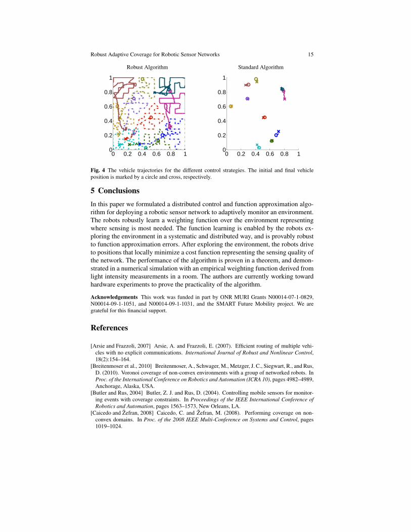
The proposed robust algorithm was compared against the standard algorithmfrom [Schwager et al., 2009], which assumes that the weighting function can bematched exactly. The true and optimally reconstructed (according to (5)) weightingfunctions are shown in Figure 3(a) and (b), respectively. As shown in Figure 3(c)and (d), with the robust and standard algorithm respectively, the proposed robustalgorithm significantly outperforms the standard algorithm and reconstructs the trueweighting function well. The robot trajectories for the robust and standard adaptivecoverage algorithm are shown in Figure 4(a) and (b), respectively. Since the standardalgorithm doesn’t include the exploration phase, the robots get stuck in a local areaaround their starting position which causes the robots to be unsuccessful in learningan acceptable model of the weighting function. In contrast, the robots with the ro-bust algorithm explore the entire space and reconstruct the true weighting functionwell.

True Weighting Function Optimally Reconstructed

Robust Algorithm Standard Algorithm

Fig. 3 A comparison of the weighting functions. (a) The true weighting function. (b) The optimallyreconstructed weighting function for the chosen basis functions. (c) The weighting function for theproposed algorithm with deadzone and exploration. (d) The previously proposed algorithm withoutdeadzone or exploration.


Robust Algorithm Standard Algorithm

0 0.2 0.4 0.6 0.8 10

0.2

0.4

0.6

0.8

1

0 0.2 0.4 0.6 0.8 10

0.2

0.4

0.6

0.8

1

Fig. 4 The vehicle trajectories for the different control strategies. The initial and final vehicleposition is marked by a circle and cross, respectively.

5 ConclusionsIn this paper we formulated a distributed control and function approximation algo-rithm for deploying a robotic sensor network to adaptively monitor an environment.The robots robustly learn a weighting function over the environment representingwhere sensing is most needed. The function learning is enabled by the robots ex-ploring the environment in a systematic and distributed way, and is provably robustto function approximation errors. After exploring the environment, the robots driveto positions that locally minimize a cost function representing the sensing quality ofthe network. The performance of the algorithm is proven in a theorem, and demon-strated in a numerical simulation with an empirical weighting function derived fromlight intensity measurements in a room. The authors are currently working towardhardware experiments to prove the practicality of the algorithm.

Acknowledgements This work was funded in part by ONR MURI Grants N00014-07-1-0829,N00014-09-1-1051, and N00014-09-1-1031, and the SMART Future Mobility project. We aregrateful for this financial support.

References

[Arsie and Frazzoli, 2007] Arsie, A. and Frazzoli, E. (2007). Efficient routing of multiple vehi-cles with no explicit communications. International Journal of Robust and Nonlinear Control,18(2):154–164.

[Breitenmoser et al., 2010] Breitenmoser, A., Schwager, M., Metzger, J. C., Siegwart, R., and Rus,D. (2010). Voronoi coverage of non-convex environments with a group of networked robots. InProc. of the International Conference on Robotics and Automation (ICRA 10), pages 4982–4989,Anchorage, Alaska, USA.

[Butler and Rus, 2004] Butler, Z. J. and Rus, D. (2004). Controlling mobile sensors for monitor-ing events with coverage constraints. In Proceedings of the IEEE International Conference ofRobotics and Automation, pages 1563–1573, New Orleans, LA.

[Caicedo and Zefran, 2008] Caicedo, C. and Zefran, M. (2008). Performing coverage on non-convex domains. In Proc. of the 2008 IEEE Multi-Conference on Systems and Control, pages1019–1024.


[Choset, 2001] Choset, H. (2001). Coverage for robotics—A survey of recent results. Annals ofMathematics and Artificial Intelligence, 31:113–126.

[Cortes et al., 2005] Cortes, J., Martınez, S., and Bullo, F. (2005). Spatially-distributed coverageoptimization and control with limited-range interactions. ESIAM: Control, Optimisation andCalculus of Variations, 11:691–719.

[Cortes et al., 2004] Cortes, J., Martınez, S., Karatas, T., and Bullo, F. (2004). Coverage controlfor mobile sensing networks. IEEE Transactions on Robotics and Automation, 20(2):243–255.

[Drezner, 1995] Drezner, Z. (1995). Facility Location: A Survey of Applications and Methods.Springer Series in Operations Research. Springer-Verlag, New York.

[Duda et al., 2001] Duda, R., Hart, P., and Stork, D. (2001). Pattern Classification. Wiley andSons, New York.

[Ioannou and Kokotovic, 1984] Ioannou, P. and Kokotovic, P. V. (1984). Instability analysis andimprovement of robustness of adaptive control. Automatica, 20(5):583–594.

[Latimer IV et al., 2002] Latimer IV, D. T., Srinivasa, S., Shue, V., adnd H. Choset, S. S., andHurst, A. (2002). Towards sensor based coverage with robot teams. In Proceedings of the IEEEInternational Conference on Robotics and Automation, volume 1, pages 961–967.

[Lloyd, 1982] Lloyd, S. P. (1982). Least squares quantization in pcm. IEEE Transactions onInformation Theory, 28(2):129–137.

[Martınez, 2010] Martınez, S. (2010). Distributed interpolation schemes for field estimation bymobile sensor networks. IEEE Transactions on Control Systems Technology, 18(2):419–500.

[Narendra and Annaswamy, 1987] Narendra, K. and Annaswamy, A. (1987). A new adaptive lawfor robust adaptation without persistent excitation. Automatic Control, IEEE Transactions on,32(2):134 – 145.

[Narendra and Annaswamy, 1989] Narendra, K. S. and Annaswamy, A. M. (1989). Stable Adap-tive Systems. Prentice-Hall, Englewood Cliffs, NJ.

[Ogren et al., 2004] Ogren, P., Fiorelli, E., and Leonard, N. E. (2004). Cooperative control ofmobile sensor networks: Adaptive gradient climbing in a distributed environment. IEEE Trans-actions on Automatic Control, 49(8):1292–1302.

[Peterson and Narendra, 1982] Peterson, B. and Narendra, K. (1982). Bounded error adaptivecontrol. IEEE Transactions on Automatic Control, 27(6):1161 – 1168.

[Pimenta et al., 2008a] Pimenta, L. C. A., Kumar, V., Mesquita, R. C., and Pereira, G. A. S.(2008a). Sensing and coverage for a network of heterogeneous robots. In Proceedings of theIEEE Conference on Decision and Control, Cancun, Mexico.

[Pimenta et al., 2008b] Pimenta, L. C. A., Schwager, M., Lindsey, Q., Kumar, V., Rus, D.,Mesquita, R. C., and Pereira, G. A. S. (2008b). Simultaneous coverage and tracking (SCAT)of moving targets with robot networks. In Proceedings of the Eighth International Workshop onthe Algorithmic Foundations of Robotics (WAFR 08), Guanajuato, Mexico.

[Samson, 1983] Samson, C. (1983). Stability analysis of adaptively controlled systems subject tobounded disturbances. Automatica, 19(1):81 – 86.

[Sastry and Bodson, 1989] Sastry, S. S. and Bodson, M. (1989). Adaptive control: stability, con-vergence, and robustness. Prentice-Hall, Inc., Upper Saddle River, NJ.

[Schwager et al., 2008] Schwager, M., McLurkin, J., Slotine, J. J. E., and Rus, D. (2008). Fromtheory to practice: Distributed coverage control experiments with groups of robots. In Experi-mental Robotics: The Eleventh International Symposium, volume 54, pages 127–136. Springer-Verlag.

[Schwager et al., 2009] Schwager, M., Rus, D., and Slotine, J. J. (2009). Decentralized, adaptivecoverage control for networked robots. International Journal of Robotics Research, 28(3):357–375.

[Schwager et al., 2011] Schwager, M., Rus, D., and Slotine, J. J. (2011). Unifying geometric,probabilistic, and potential field approaches to multi-robot deployment. International Journal ofRobotics Research, 30(3):371–383.

[Slotine and Li, 1991] Slotine, J. J. E. and Li, W. (1991). Applied Nonlinear Control. Prentice-Hall, Upper Saddle River, NJ.

[Weber, 1929] Weber, A. (1929). Theory of the Location of Industries. The University of ChicagoPress, Chicago, IL. Translated by Carl. J. Friedrich.

Robust Adaptive Coverage for Robotic Sensor...

Documents

Transcript of Robust Adaptive Coverage for Robotic Sensor...