Robotic Motion Planning: Potential Functions and Search

16-735, Howie Choset, with slides from Ji Yeong Lee, G.D. Hager and Z. Dodds

Robotic Motion Planning:Potential Functions and Search

Robotics Institute 16-735http://voronoi.sbp.ri.cmu.edu/~motion

Howie Chosethttp://voronoi.sbp.ri.cmu.edu/~choset


The Basic Idea

Compute Distance• Polygon• Sensor• Grid

Local Minima• Wavefront• Navigation Function


Diffeomorphism vs. Homeomorphism

HOMEOMORPHISM

DIFFEOMORPHISM


Potential Fields on Non-Euclidean Spaces

• Thus far, we’ve dealt with points in Rn --- what about real manipulators

• Recall we can think of the gradient vectors as forces -- the basic idea is to define forces in the workspace (which is ℜ2 or ℜ3)

Power in configuration space

Power in work space

Power is conserved!


Force on an Object

torque


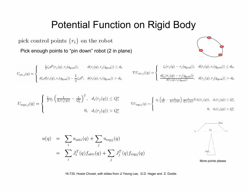
Potential Function on Rigid Body

Pick enough points to “pin down” robot (2 in plane)

More points please


Potential Fields for Multiple Bodies

• Recall we can think of the gradient vectors as forces -- the basic idea is to define forces in the workspace (which is ℜ2 or ℜ3)

– We have Jt f = u where f is in W and u is in Q– Thus, we can define forces in W and then map them to Q

– Example: our two-link manipulator

α

β

L1

L2

(x,y)

y

x

x L1cα L2cα+β

y L1sα L2sα+β

= +


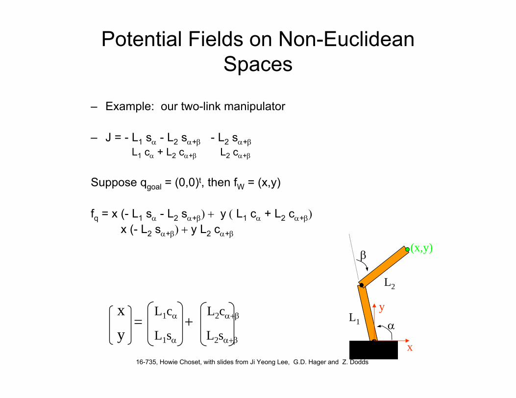
Potential Fields on Non-Euclidean Spaces

– Example: our two-link manipulator

– J = - L1 sα - L2 sα+β - L2 sα+βL1 cα + L2 cα+β L2 cα+β

Suppose qgoal = (0,0)t, then fW = (x,y)

fq = x (- L1 sα - L2 sα+β) + y ( L1 cα + L2 cα+β)x (- L2 sα+β) + y L2 cα+β

α

β

L1

L2

(x,y)

y

x

x L1cα L2cα+β

y L1sα L2sα+β

= +


In General

• Pick several points on the manipulator

• Compute attractive and repulsive potentials for each

• Transform these into the configuration space and add

• Use the resulting force to move the robot (in its configuration space)

α

β

L1

L2

(x,y)

y

x

RF4

RF3

RF2

RF1

AF1

Be careful to use the correct Jacobian!


Summary

• Basic potential fields– attractive/repulsive forces

• Gradient following and Hessian

• Navigation functions

• Extensions to more complex manipulators


Outline

• Overview of Search Techniques• A* Search• D* Search


Graphs

Collection of Edges and Nodes (Vertices)

A tree


Search in Path Planning

• Find a path between two locations in an unknown, partially known, or known environment

• Search Performance– Completeness– Optimality → Operating cost– Space Complexity– Time Complexity


Search

• Uninformed Search– Use no information obtained from the environment– Blind Search: BFS (Wavefront), DFS

• Informed Search– Use evaluation function– More efficient– Heuristic Search: A*, D*, etc.


Uninformed Search

Graph Search from A to N

BFS


Informed Search: A*

Notation• n → node/state• c(n1,n2) → the length of an edge connecting between n1 and n2

• b(n1) = n2 → backpointer of a node n1 to a node n2.


Informed Search: A*

• Evaluation function, f(n) = g(n) + h(n)• Operating cost function, g(n)

– Actual operating cost having been already traversed• Heuristic function, h(n)

– Information used to find the promising node to traverse– Admissible → never overestimate the actual path cost

Cost on a grid


A*: Algorithm

The search requires 2 lists to store information about nodes

1) Open list (O) stores nodes for expansions

2) Closed list (C) stores nodes which we have explored


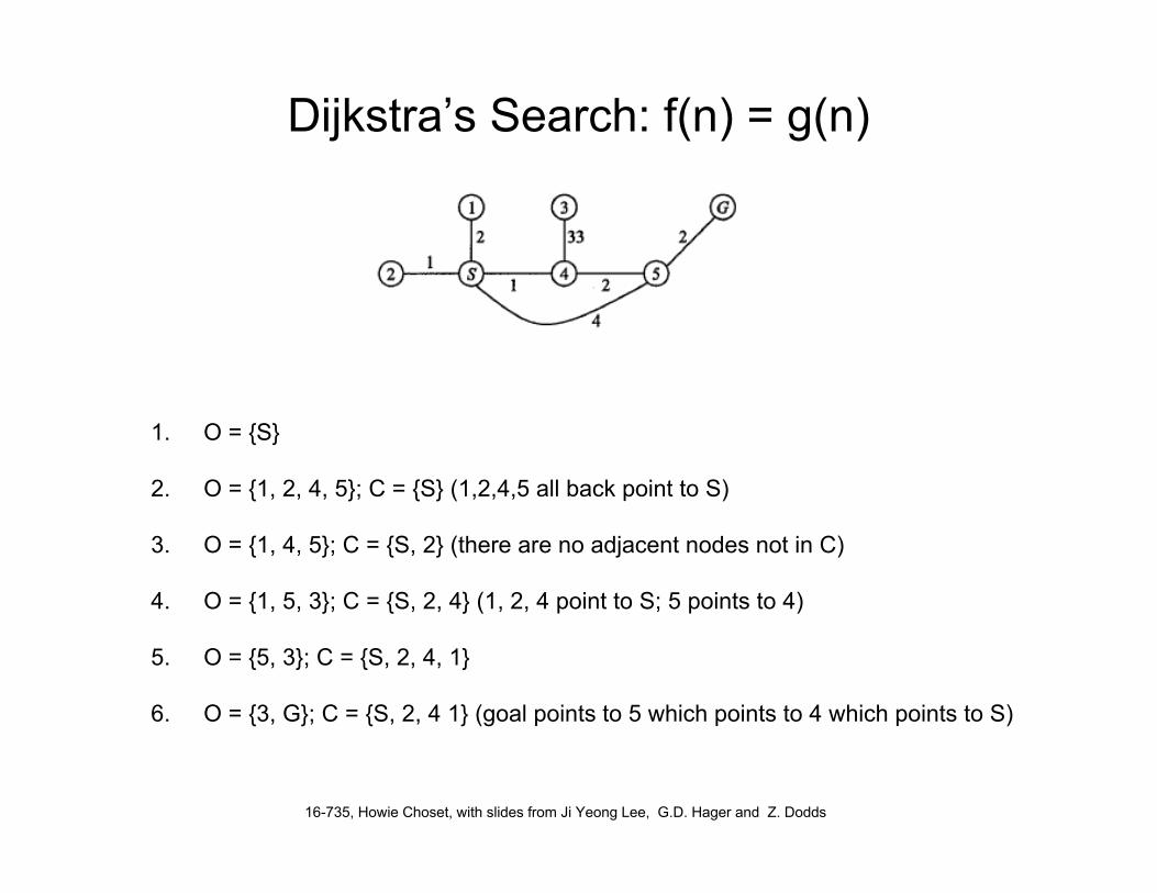
Dijkstra’s Search: f(n) = g(n)

1. O = {S}

2. O = {1, 2, 4, 5}; C = {S} (1,2,4,5 all back point to S)

3. O = {1, 4, 5}; C = {S, 2} (there are no adjacent nodes not in C)

4. O = {1, 5, 3}; C = {S, 2, 4} (1, 2, 4 point to S; 5 points to 4)

5. O = {5, 3}; C = {S, 2, 4, 1}

6. O = {3, G}; C = {S, 2, 4 1} (goal points to 5 which points to 4 which points to S)


Two Examples Running A*

GOAL

33 3

3

3

3 3

1

1 22

3

3

3

2

2

0 Start

2

241

1

1 1

1

1 1

1 1

A

B

CD

E F

G H I

J K

L


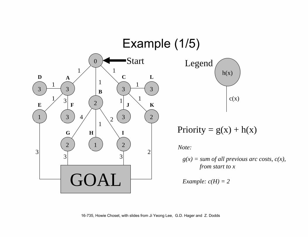
Example (1/5)

h(x)

c(x)

Legend

Priority = g(x) + h(x)

g(x) = sum of all previous arc costs, c(x),from start to x

Example: c(H) = 2GOAL

33 3

3

3

3 3

1

1 22

3

3

3

2

2

0 Start

2

241

1

1 1

1

1 1

1 1

A

B

CD

E F

G H I

J K

L

Note:


Example (2/5)

C(4)

A(4)

B(3)

A(4)

I(5)

G(7)

C(4)

H(3)

First expand the start node

If goal not found,expand the first nodein the priority queue(in this case, B)

Insert the newly expandednodes into the priority queueand continue until the goal isfound, or the priority queue isempty (in which case no pathexists)

Note: for each expanded node,you also need a pointer to its respectiveparent. For example, nodes A, B and Cpoint to Start

GOAL

33 3

3

3

3 3

1

1 22

3

3

3

2

2

0 Start

2

241

1

1 1

1

1 1

1 1

A

B

CD

E F

G H I

J K

L


Example (3/5)

C(4)

A(4)

B(3)

A(4)

I(5)

G(7)

C(4)

H(3) No expansion

F(7)

C(4)

I(5)

G(7)

D(5)

E(3) GOAL(5)

We’ve found a path to the goal:Start => A => E => Goal(from the pointers)

Are we done?GOAL

33 3

3

3

3 3

1

1 22

3

3

3

2

2

0 Start

2

241

1

1 1

1

1 1

1 1

A

B

CD

E F

G H I

J K

L


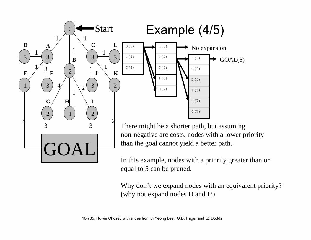
Example (4/5)

C(4)

A(4)

B(3)

A(4)

I(5)

G(7)

C(4)

H(3) No expansion

F(7)

C(4)

I(5)

G(7)

D(5)

E(3) GOAL(5)

There might be a shorter path, but assumingnon-negative arc costs, nodes with a lower prioritythan the goal cannot yield a better path.

In this example, nodes with a priority greater than orequal to 5 can be pruned.

Why don’t we expand nodes with an equivalent priority?(why not expand nodes D and I?)

GOAL

33 3

3

3

3 3

1

1 22

3

3

3

2

2

0 Start

2

241

1

1 1

1

1 1

1 1

A

B

CD

E F

G H I

J K

L


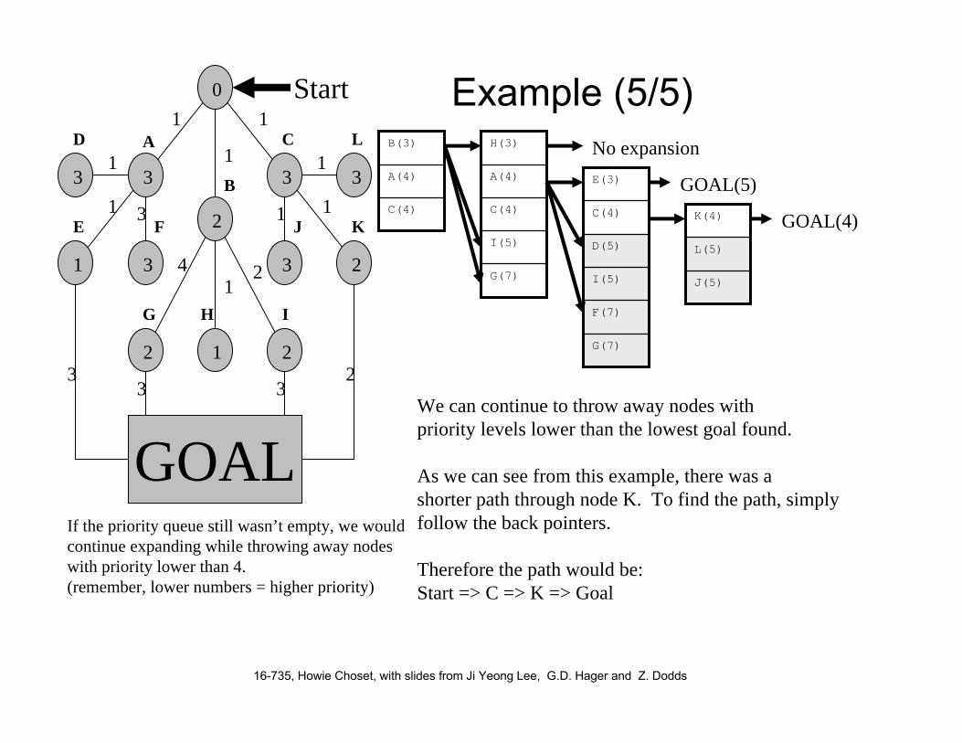
Example (5/5)

C(4)

A(4)

B(3)

A(4)

I(5)

G(7)

C(4)

H(3) No expansion

F(7)

C(4)

I(5)

G(7)

D(5)

E(3) GOAL(5)

We can continue to throw away nodes withpriority levels lower than the lowest goal found.

As we can see from this example, there was ashorter path through node K. To find the path, simplyfollow the back pointers.

Therefore the path would be:Start => C => K => Goal

L(5)

J(5)

K(4) GOAL(4)

If the priority queue still wasn’t empty, we wouldcontinue expanding while throwing away nodeswith priority lower than 4.(remember, lower numbers = higher priority)

GOAL

33 3

3

3

3 3

1

1 22

3

3

3

2

2

0 Start

2

241

1

1 1

1

1 1

1 1

A

B

CD

E F

G H I

J K

L


Assign Final Project

• Must have a filtering component (e.g., Kalman, Bayes)• Work on a real robot

Create a PPT• Title, Name, Photo of you, Photo of Robot• What your project is going to do• Which filtering technique and why• How you are going to demonstrate result

Robotic Motion Planning: Potential Functions and Search

Documents

Transcript of Robotic Motion Planning: Potential Functions and Search