ROBOTIC MANIPULATOR THROUGH THE USE OF -iM … · -im 933 positioning of a robotic manipulator...

-iM 933 POSITIONING OF A ROBOTIC MANIPULATOR THROUGH THE USE OF 1/2

VISUAL FEEDBACK(U) AIR FORCE INST OF TECHNRIGHT-PATTERSON AF9 OH N T O'DONNELL MAY 85

UNCLASSIFIED AFIT/CI/NR-85-2T F/G 6/4 M

2.

11111_L25

W ~ ~ ~ ~ c It!P ll2L21(

.. - ...- -..-. . , . . ;. . . . j . ' ; , ; - . • ': .* - ' W ' ' - • '

" " ' " '-• '

. . . A hU iLLA S ... ..... . ... ......

S-LI(IJAITY CL ASSiFIl, AlI).N 4, T. I' A(, l .n.

REP3RI DOUM=, .TIC . AE .,.,: ,'MI ~.lvl -. IMIIH A .I A N I' A AL n r-MiLL

=i / J' j'[ '

. .'' 2 0 T4 TIIL I .-,1. 2OT- b P- O HI, PUR1 & ~ kL , NI O VL t DN

Positioning Of A Robotic Manipulator Through The I.i -SI ,L.V lf/1Y YyVUse Of Visual Feedback

PI FO(MNG(.:;G.RLP.(.)HT" NUMULIR.

7Aul THUN(. P, CONTRACT OR LRANT NumaER(a)

Maurice Thomas O'Donnell

I /,, _ -LA CHA UNI- N,.- ..; ERt-' A

I A STUDENT AT: University of New Hampshire

~'V Cn TOL LING OFF ICE NAME ANU A0CDNLSS 12, REPORT DATE

(v AF!T/NR __y_____

WPAFB OH ,133 3. NUMBER OF PAGES113 __

4 M., 4 ITONIIJ(. Al.N , NAM[ A Ar,OHLs(i I..l,,a t,,l, ,,,,Ir.IIrl nih' 3) C iS. ko ,sECURITY CLA'.:. (oI lhi. P'p t)

* ln UNCLASS",15a. "DE (:L ASSIFICAT I)N DOWNGRAD)ING

S C I-EDU L E

L, ,-%TH 1 1, N ~TA T LM EN'T i t hI x H P~lr 1)

&PI'kUVHu !OR PUBLIC RLLEASE; DISTRIBUTION UNLIMITE,

tH . E 'At N TAil NOT!

API'UVLD fOR PUBLIC RELLASE: IAw AFR 1'0-, L';-N L. WOLAvLR - I -

Dean for Research andS Prufessio Ievelopmen

A rji ht -'atterson AF6 OH

71-1

---'--J ~ l " 4i.(g,.V '

0

,AN I 1 4/ '" ' ..... ... !JNCLA~jS

85 0 3 0.l- 4 "6" " " " T

q

2MAT IURICE O'DONNELl,USAF10)85

113 pages". S. ELICTRICAL ENGINEERINGENIVE.RSITY OF NEW IAMPSI!IRE

F : , "T

"T!.

-1\,J I'

A'*

POSITIONING OF A ROBOTIC MANIPULATOR

THROUGH THE USE OF VISUAL FEEDBACK

By

Maurice Thomas O'Donnell

B.S., University of New Hampshire, 1983

A THESIS

Submitted to the University of New Hampshire

in Partial Fulfillment of

the Requirements for the Degree of

Master of Science

in

Electrical Engineering

May, 1985

.I IJ

This thesis has been examined and approved.]

Thesis director, Filson H. Ga/4 Associate Professor of Electrical and

Computer Engineering

W. Thomas Miller, Associate Professor ofElectrical and Computer Engineering

I Gordon Kraft, Associate P*ofessor ofElectrical and Computer Engineering

Date

I p

I -1

e1

I .1

.]

ACKNOWLEDGEMENTS

I would like to express my sincere appreciation to Professor

Filson H. Glanz who generously gave much time and thought to helping me

complete this thesis research. I would also like to express my gratitude

to the United States Air Force for providing the means by which I could

afford to receive both my undergraduate and graduate degrees and still

provide for the needs of my family. Above all I would like to give

special thanks to my family; Linda, Michael, Kerilyn, and Jennifer who

put up with an absent father and husband on many important occasions

during the last four and one-half years with few complaints. In

addition I would like to thank them for some very happy memories and

giving me a place I enjoyed calling 'home'

iii

TABLE OF CONTENTS

ACKNOWLEDGEMENTS i--------------------------------------------i

LIST OF TABLES ---------------------------------------------- vi

LIST OF FIGURES --------------------------------------------- vii

ABSTRACT -------------------------------------------------------- ix

CHAPTER I INTRODUCTION ----------------------------------------- 1

CHAPTER II IMAGE ACQUISITION AND PROCESSING --------------------- 7

Computer Vision Systems---------------------------7

Static Scene Analysis ---------------------------- 16

Dynamic Scene Analysis --------------------------- 20

Equipment Used in the Study ----------------------- 22

Processing Technique Employed --------------------- 24

CHAPTER III ROBOTIC MANIPULATOR KINEMATICS ---------------------- 31

Forward Kinematics ------------------------------ 32

Forward Kinematics for P-5 Robot ------------------ 47

* Inverse Kinematics ------------------------------ 51

Inverse Kinematics for P-5 Robot ------------------ 53

Calibration of Camera to Robot -------------------- 57

Components of the System ------------------------- 59

The Estimation Used in the Demonstration Task 62

CHAPTER IV EXPERIMENTAL RESULTS AND ANALYSIS -------------------- 67

Experiments and Results -------------------------- 67

Model for Experimental Results -------------------- 75

CHAPTER V CONCLUSIONS AND FUTURE RESEARCH ----------------------- 82

Suggestion for Future Research -------------------- 83

iv

*q

REFERENCES------------------------------------------------------- 89

APPENDIX A: LEAST SQUARES CALIBRATION METHOD AND SOFTWARE LISTING- 92

APPENDIX B: COMPUTER PROGPAM LISfING ----------------------------- 100m

LIST OF TABLES

TABLE PAGE

3.1 P-5 Robot Joint Parameters ---------------------------- 48

4.1 Image Processing Error Data --------------------------- 70

4.2 Overall System Error Test Data ------------------------ 74

4.3 General Discrete Kalman Filter ------------------------ 77

vi

0 i

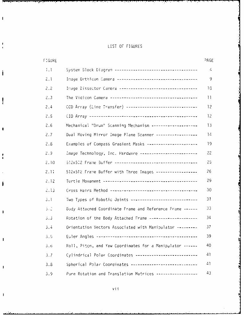
LIST OF FIGURES

FIGURE PAGE

1.i System Block Diagram -------------------------------------- 4

2.1 Image Orthi con Camera ------------------------------------- 9

2.2 Image Dissector Camera ------------------------------------ 10

2.3 The Vidicon Camera ---------------------------------------- 11

2.4 CCD Array (Line Transfer)--------------------------------- 12

2.5 CID Array------------------------------------------------ 12

2.6 Mechanical "Drum" Scanning Mechanism ---------------------- 13

2.7 Dual Moving Mirror, Image Plane Scanner -------------------- 14

2.8 Examples of Compass Gradient Masks-------------------------19

2.9 Image Technology, Inc. Hardware --------------------------- 22

2.10 1 2x512 Frame Buffer -------------------------------------- 25

2.11 512x512 Frame Buffer with Three Images -------------------- 26

2.12 Turtle Movement------------------------------------------ 29

2.13 Cross Hairs Method ---------------------------------------- 30

3.1 Two Types of Robotic Joints ------------------------------- 31

Body Attached Coordinate Frame and Reference Frame ---- 33

J3.3 Rotation of the Body Attached Frame ----------------------- 34

3.4 Orientation Vectors Associated with Manipulator ------------ 37

3.5 Euler Angles--------------------------------------------- 39

3.6 Roll, Pitch, and Yaw Coordinates for a Manipulator ---- 40

3.7 Cylindrical Polar Coordinates-----------------------------41

3.8 Spherical Polar Coordinates------------------------------- 41

3.9 Pure Rotation and Translation Matrices---------------------43

vii

FIGURE PAGE

3.10 Joint Variables and Quantities -------------------------- 46

3.11 Five Link Robot Similar to the P-5 Process Robot --------- 48

3.12 P-5 Robot, Vidicon Camera, Laser ------------------------ 57

3.13 Block Diagram of System -------------------------------- 59

3.14 Estimation Technique ----------------------------------- 64

4.1 Variance of Error in Estimation as a Function of

Prediction Time ----------------------------------- 76

4.2 Kalman Filter Estimates and Experimental Observations

for Circular Motion ------------------------------- 80

4.3 Circular Motion Prediction Using Linear Predictive

Algorithm ---------------------------------------- 81

.1 Averaging Technique for floise Problem ------------------- 35

D.2 limage Field at Two Different Heights -------------------- 37

ABSTRACT

POSITIONING OF A ROBOTIC MANIPULATOR

THROUGH THE USE OF VISUAL FEEDBACK

by

MAURICE THOMAS O'DONNELL

University of New Hampshire, May, 1985

A system for positioning a general purpose industrial robot by

4means of information extracted by a computer vision system is described.

The specific example implemented was the interception of a moving object

by a robotic manipulator based on three sequential images of the object.

The techniques used and constraints imposed are discussed. The robot

used is an industrial G.E. P-5 robot with five degrees of freedom.

Several experiments used to evaluate the various components of system

error were run. The results of these experiments were compared to the

behavior of a linear predictive Kalman filter model of the system. A

list of conclusions is presented along with a discussion of particular

areas where improvements on this system can be made. A listing of the

Fortran programs used and an outline of the camera-robot coordinate

system calibration process are included in the appendices.

ix

CHAPTER I

INTRODUCTION

The underlying objective of this project is to direct the movement

of a robotic manipulator using information acquired through an image

acquisition system. As an example of such a movement, a robotic

manipulator is driven to intercept a moving object. The prediction of

the object's position at a fixed future time is based on spacial infor-

mation extracted from three sequential images of the moving object.

For the most part in today's industrial workplace robots are per-

forming what seems to be rather trivial tasks. That is, tasks consisting

of maneuvers that can be played back over and over again. Possibly this

could be the primary reason why industry has been the ground breaking

(irea ror use of robotic manipulators. This is because a majority of

induxstrial tasks are clearly repetitive and can be expressed as a

2.jeme of fixed motions [Horn and Ikeuchi, 1984]. Tasks that have

, nidered tedious, boring, or even hazardous, such as spray paint-

,.iolng, ind part manipulation have been the perfect opportunity to

' rjot tecnnology. The particular maneuvers could be taught to

t oe <aDut by 'moving the robot through the sequence of motions while the

,;)Dot -ontrol facilities would store the sequence in some type of memory.

Tnen erely by running the stored information through a loop the robot

would be ,ble to proceed with little human intervention.

ne drawbai-k with these maneuvers is that when the environment

in some way the system breaks down rather quickly. For example,

,ne d> O O t in . speci i , ay to yiel d o d i i -ti1 na infor-

atio r to better urde r or L I or i 0 he in' frma ion tid s is a ready

o tob mu;

ril } I , he ,u. tput device presents tnis new d tf, ir, 5 T0 for:m to

J, ,3t_,J thie .) erdtor. It may consist or a onitor vin h s i / 0 I, -

oiays tO.e 'i. tio o I age. -urtnerl -ore, i ' -he output is i forxr'ati

..n lase te ,i'jnai iay be given to any one of a large grnu[) of

.evi is, su~n us i :ntrol ler, a robot, a burglar alarm, a colmlunications

n anrle an d SO oan.

e, en discussing te i mage signal in monitors or television screens,

iere are some standard features. Te image or scene on a televisio

sa.reen is due to the preserce of an electron beam striking a phosphorous

_Jdt'ing. T1hat is, the gray level of the particular point in the scene

decends on the intensity of the electron beam at that point. It is

oirly ot.ndard for the electron beam to be moved from >eft tC r1-::t !',d

tp;+ to bottom. The term 'field' has been applied to the image prodj ed

by sequence of 2621, horizontal scans lines at a rate of 60 Oties or

en O LIanin, 19'3]. By interlacing two such fields into a single i'

single frame is generated. The frame rate is therefore approxi atel .

ra es per second. This rate prevents the appearance of flicker in tie

scene becduse the iumdn visual system is able to sustain the image

Letween trames.

*bviusiy, the ability for the monitor or television receiver to

,,.pridui.e the jage acquired by the camera depend in large Dart on

.. netner the scanning systems of the camera and receiver are in 'sync'.

Tis nchronization is performed by the generati)n of synthetic video

,na is y One _a[sera .it arti calar timing spots. These timing spots

Id3Y-DEFLCTIGNSENSING ELEMENT

APERPTURE

d2 IMAGE

I F LANE

MAGNIFICATION 2 l~?+ 3 /0

x=(d ±d ) Tan 2!*

y=d 3 Tan 2#

-igure 27 "-Ad] M',oving Iirror P'age Plane Scamier [Castlemran, 1979]

ne current technnology of digitizers, as was stated before, will

t-ake an analog signal and quantize it through an analog-to-digital con-

verter and t-hen store the information in some type of semiconductor

'eroy. or the reader interested in the A1'D and quantization infor-

ation Hoescenele's text [Hoeschele, 1968] presents a complete presentation

in tne ,Abject. For those concerned with use and types of semiconductor

;iemory Muruga's text [Muroga, 198112] presents an adequate discussion in

Thnis area.

"At this point in tue, process tnere is available to t-he user a two-

,limensional representation of the image or scene located in a semi-

,_onduit'or meor ini ch Kan now be processed by the c omputer. It is

,bvious Thiat t-,f- air tdS ! -~t'hr ,o ,puter in the vision system is, to

13

Some popular mechanical scanning devices are described below.

Mechanical Drum: With this device the image is wrapped around a

cylindrical drum. The image is then rotated past a stationary aperture.

The aperture is moved by way of a lead-screw. After an entire line is

digitized the lead screw is repositioned. This process is repeated

until the entire image is scanned [Figure 2.6].

IMAGE ROTATING DRUM

7 MOTOR

CARRIER LEAD SCREW

Figure 2.6 Mechanical "Drum" Scanning Mechanism [Castleman, 1979]

Flat bed scanner: This device is similar to the drum system,

however the image is placed on a flat bed. In this structure either the

ned or the image is repositioned in the digitizing process.

Laser scanner: A source of light (laser) and a mirror configuration

are used to obtain a planar image. The mirrors are connected physically

tu galvanometers, which are driven by external sources, to provide

deflection in the x or y direction [Figure 2.7].

12

VIDEO OUT OUTPUT AMP

TRANSMISSION OU TPUT SHIFTGATES REGISTER

PHOTOSENSITIVEARRAY

L " -VERTICALSCANGENERATOR

FHORIZONTAL CLOCK

igure L.- ECD A:rdy (Line Transfer) [Ballard and Brown, 1982]

LPHOTOSENSITIVE ELEMENT

VERTICAL CHARGING TRANSFERGENE RATC1R HOLDING ELEMENTS

[I

HORIZONTAL REGISTER VIDEO OUT

Figure .5 CID Array [Ballard and Brown, 1982]

PF'OTUCONDUCTIVE THERMIONIC

TARGET CATHODE

MESH

SIGNAL SIGNAL

PLATE CURRENT BEAM CURRENT

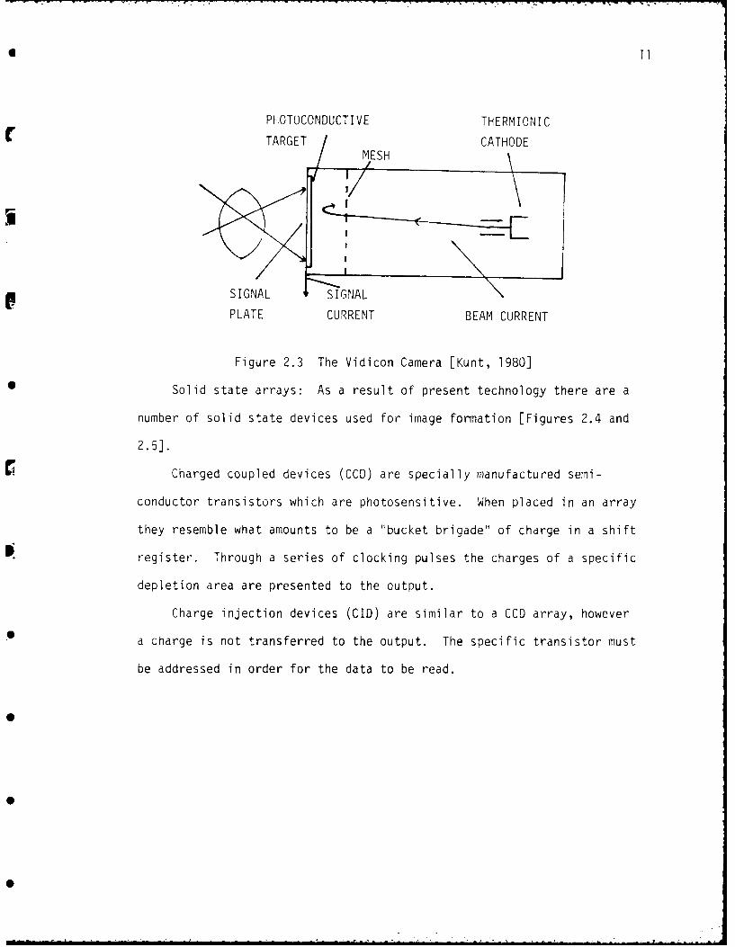
Figure 2.3 The Vidicon Camera [Kunt, 1980]

Solid state arrays: As a result of present technology there are a

number of solid state devices used for image formation [Figures 2.4 and

2.5].

Charged coupled devices (CCD) are specially manufactured semi-

conductor transistors which are photosensitive. When placed in an array

they resemble what amounts to be a "bucket brigade" of charge in a shift

register. Through a series of clocking pulses the charges of a specific

depletion area are presented to the output.

Charge injection devices (CID) are similar to a CCD array, however

a charge is not transferred to the output. The specific transistor must

be addressed in order for the data to be read.

0

, -=J ..

S. . .- - • - ' - ' - "-" - " • • .. . - .- . - . - .-.- .. °- . - .. -- -.- - •-~

10I0 "

current at the rear of the tube is the difference between the scanning

current and the locally absorbed current.

Image dissector tube: Here light from an object is focused on a

photocathode which converts photon energy into electron flow. Only those

electrons emitted from a specific area of the cathode are deflected into

an aperture and reach a photo multiplier. The spectral range of the

image dissector is from ultraviolet to infrared (Figure 2.2).

PH TOCATHODE APERTURE PLATE

ELECTRON IMAGE ELECTRON MULTIPLIER

Figure 2.2 Image Dissector Camera [Kunt, 1980]

The vidicon: This device converts the energy of incoming photons

to an electron flow through a photoconductive target. The target is

coated witn an emulsion whose resistance decreases when illuminated. An

electron beam is scanned on the back side of this target. Due to the

capacitance the charges are held by the target. The result is a capacitive

current which is used as the video signal [Figure 2.3].

*

6 9

ation of these two. It allows for the object to be illuminated

by a moving spot and sampled through a moving aperture. Such

a system is obviously complex and so has had limited use

[Castleman, 1979].

Some of the popular electronic scanning devices are described below.

Image orthicon camera: This system (Figure 2.1) has several

sections. Light from the scene is focused onto a photocathode. The

ELECTRON IMAGEPHOTOCATHODE TARGET ELECTRON MULTIPLIER

B EAM SIGNALU CURRENT

I RETURNT"-

C THERMIONIC CATHODE

Figure 2.1 Image Orthicon Camera [Kunt,1980]

photocathode in turn emits a number of electrons proportional to the light

intensity toward a positively charged target. This second target,

* which consists of a thin glass disk with a wire grid facing the photo-

cathode, will produce a secondary emission when struck by the electrons.

As a result, a positive charge begins to build up on the photocathode

* side of the second target. The back side of the disk is continuously

scanned by a moving electron beam. The disk absorbs these electrons in

a neutralizing process. The areas of high intensity will use a large

* number of electrons to neutralize this part of the target. The output

8

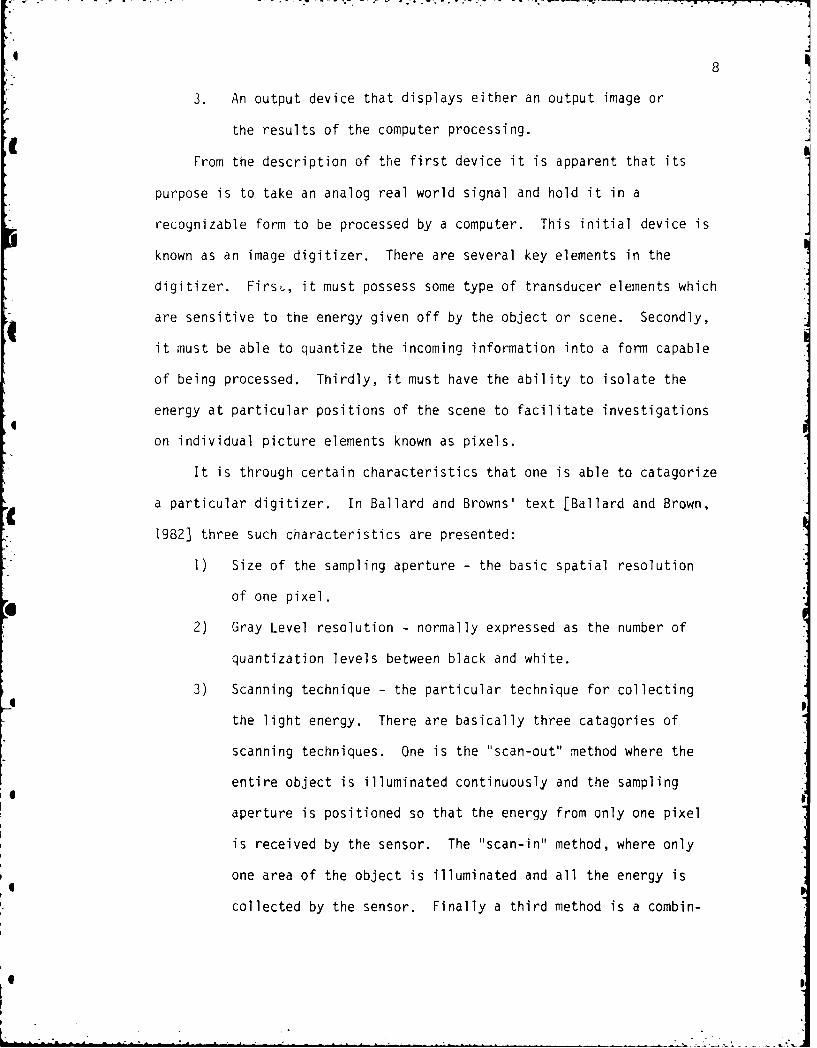
3. An output device that displays either an output image or

the results of the computer processing.j

From the description of the first device it is apparent that its

purpose is to take an analog real world signal and hold it in a

recognizable form to be processed by a computer. This initial device is

known as an image digitizer. There are several key elements in the

digitizer. Firsu, it must possess some type of transducer elements which

are sensitive to the energy given off by the object or scene. Secondly,

it must be able to quantize the incoming information into a form capable

of being processed. Thirdly, it must have the ability to isolate the

energy at particular positions of the scene to facilitate investigations

on individual picture elements known as pixels.

It is through certain characteristics that one is able to catagorize

a particular digitizer. In Ballard and Browns' text [Ballard and Brown,

1982] three such characteristics are presented:

1) Size of the sampling aperture - the basic spatial resolution

of one pixel.

2) Gray Level resolution - normally expressed as the number of

quantization levels between black and white.

3) Scanning technique - the particular technique for collecting

the light energy. There are basically three catagories of

scanning techniques. One is the "scan-out" method where the

entire object is illuminated continuously and the sampling

aperture is positioned so that the energy from only one pixel

is received by the sensor. The "scan-in" method, where only

one area of the object is illuminated and all the energy is

collected by the sensor. Finally a third method is a combin-

I

( CHAPTER II

IMAGE ACQUISITION AND PROCESSING

ro Digital image processing is an area of study that cannot be placed

under any one scientific or engineering discipline. The definitions range

from simply "...the manipulation of images by computer.. ." [Castleman,

E 1979] to more informative statements such as '"...the construction of

explicit, meaningful descriptions of physical objects from images...."

[Ballard and Brown, 1982]. It is obvious that within this second quote

lies the reason for most of the activity in this fairly new field.

Computer vision, for the purposes of this thesis, is a term used synony-

mously with digital image processing. It has proved to be a very useful

Ctool for learning additional information about the world in which we

live. The early applications of this field which included space

exploration and x-ray technology have opened doors to other fields in-

cluding robotics, pattern recognition, image graphics and so on. This

chapter presents certain facts describing techniques and equipment used

today in the field of computer vision. After this presentation the

techniques used in the study will be described.

Computer Vision Systems

I Tnere are basically three fundamental parts of any computer vision

system:

1. A device which will take and store an image.

I2. The digital computer which performs some type of processing.

7

6

In Chapter II of this thesis a brief introduction to specific

aspects of computer vision is presented. The elements of a general image

acquisition system are discussed. The specific hardware of the system

used in this research is briefly described. Finally, the image pro-

cessing techniques peculiar to this system are explained.

In Chapter III a discussion of robot configurations and kinematics

is presented. A description is given of some specific details of the

general system. The transformation from the attached camera coordinates

to the manipulator coordinates is derived. This chapter ends with a dis-

cussion of the specific estimation technique used in the example.

In Chapter IV the system performance is evaluated by means of three

experiments which were designed to quantify imaging error, positioning

error and total system error. Also introduced is a simple model using a

Kalman filter that will serve as a basis for examining the experimental

data of the system.

In Chapter V is a presentation of the conclusions of this research.

Finally, a discussion of specific improvements on the system is presented

along with an indication of future research areas that are possible with

this system.

0

-7-7 -1 .

graphical look at the major components of the system. The four

components are:

(p 1) The Supervisory Computer receives data from both the image

acquisition system and the robotic front end processor and controller.

Through the use of a high level language the supervisory computer can

examine the information concerning the existing environment and then

direct a movement of the robotic manipulator in response. The response

is delivered to the robotic front end processor and controller by means

of a serial communication line.

2) The Front End Processor and Controller performs two main

functions. The first is a command function which interprets the infor-

mation on the serial line as either data or instructions to be accomplish-

ed. The second function is that of control whereby the actual robotic

manipulator's trajectory and velocity are specified.

3) The Image Acquisition System provides digital images of the area

directly below the end-effector of the robot. These images basically

can act as a window on this area which when examined in sequence provide

dynamic information about this particular scene.

4) The Robotic Manipulator is the structure that is being directed

by the system.

The example used to test the robotic system developed in this thesis

is a simple linear tracker. The change in the environment that is being

observed is a moving object. The system monitors this object and makes

an estimate about the object's position at some point in the future.

Once the future position is calculated the system derives the necessary

information to direct the robotic manipulator to intercept this object

at the future point in time.

4

With the increased demand for intelligent robots the applications

will most certainly bring them out of the industrial area into new

expanding fields such as space exploration and deep sea mining. Possibly

any area that might present a hazard to man while necessitating a de-

cision being made will offer new areas of use for the intelligent robot.

It turns out that "computer vision, the collection of techniques...

for obtaining measurements and inferences from images, appears to offer

4 the richest source of sensory information for intelligent robotic

manipulation in the greatest number of environments" [Hall et al, 1982].

The need for vision-equipped robots is seen when estimations are presented

that a quarter of all industrial robots will be equipped with some form

of vision system [Miller, 1984].

In this research an attempt at establishing an intelligent robot

system is carried out. The block diagram seen in Figure 1.1 reveals a

FRONT-END PROCESSOR

SUPERVISORY COMPUTER and CONTROLLER

I0

MANIPULATOR WITH

CAMERA MOUNTED--

IMAGE ACQUISITIONSYSTEM

Figure 1.1 System Block Diagram

3

These reasons, and additionally the fact that numerous other tasks

could benefit, have led to the continuing development of intelligent

robots. Research in the areas of transportAtion, bin-picking, assembly,

and quality control has been on-going for the last few years. The

problems involved with transporting items from place to place in a "blind"

workplace have been stated already. The ability of an intelligent robot

to overcome these problems could help to avoid production loss due to down

time, damage to equipment and most importantly, injuries to human

operators.

Bin-Picking is a term that is applied in robotics to a situation

where a number of objects are in close proximity and the system is able to

uelirieate a particular object and then to maneuver the manipulator in such

j way ds to grasp and transport the object.

* s__embl is a term applied to a technique whereby a robot can grasp

several objects in a specific order and then orient them with reference

to eacn other in some predetermined fashion. For example, putting a nut

onto the end of a bolt or a peg into a hole. These common tasks should

not be belittled because of the complexities involved in directing such

manipulations. A simple assembly task may involve several very difficult

subtasks, such as, pattern recognition, bin-picking, and properly align-

ing the individual objects.

Finally, Quality Control, which is a repetitive examination of manu-

factured parts seems to be an excellent application for an intelligent

robot equipped with a vision capability, thus freeing the operator for

a more responsible position with much more satisfaction. This task

may run the gamut from inspection of integrated circuit boards to paint

jobs on the body of a new automobile.

..

.I

i t It ''.-U r ned path of the manipulator,

there is no Way 'I tj, + " , , 'r t, d Void the collision. With

toese "non-intel Ii jnt ' robus Ti orientation irnd initial Position of

the manipulated object, tne path ot movement and the final position must

be accomplished to very close tolerances.

It is obvious that a large number of tasks exist that are particularly

suited to application of so-called "intelligent" robots. These are robots

equipped with transducers so that changes in the environment can be de-

tected that may cause the system to falter. These robots should be

equipped to compensate for these contingencies.

Some authors are proposing that future industries will strive to

improve the organization of the workplace. This movement is working to

relieve any possibility that changes in the environment detrimental to

system performance occur. This trend is in response to the fact that for

non-intelligent robots all positions and orientations must be repetitive.

Simple tasks such as moving objects from place to place presuppose the

ability of the robot to grasp the object properly each time. Of course

this ability is dependent on the position and orientation of the object.

The proponents of this trend are advocating that storage structures for

objects be carriers and pallets rather than bins. At the present time

much research is devoted to designing devices that will perform the

positioning and orientation tasks on objects of all sizes. There are a

number of drawbacks that are evident in such a trend. First there is aI

manufacturing and design cost for these new devices. Second, if an

item is modified in any way the orientation device must also be modified.

Third,to provide orientation and position of parts may not be the most

economical way to store them. Finally, it seems an impossible task to

provide for all possible contingencies in any environment.

I

* 16

occur at the end of each horizontal scan when the camera's scanning

system must be moved back from right to left. At this time, a

horizontal blanking signal is generated by the camera so that no infor-

mation is acquired during this retrace. In addition a horizontal sync

pulse is generated at these times. basically, the presence of the

synthetic signals provide the timing information for the monitor to

lock-in on the active video signal. There is also a vertical blanking

signal that nmarks the time for the scanning system to reset itself to the

top-left position. Because of the time involved with this vertical re-

trace only about 480 out of 525 horizontal scan lines provide informat'on

to the monitor.

Static Scene Analysis

At this point we are concerned with the data as it exists in the

acquisition system. It can be viewed as an array of discrete picture

elements, whose numerical value is an indication of its shading or

gray level. The array of pixels, therefore, taken as a whole is a dis-

crete approximation of the initial scene or object. Through the use of

hardware and software algorithms the computer vision system '.. .extracts

pertinent information from the image data. This module in essence

performs the task of isolating 'interesting' areas for further

analysis" [Computer, Vol. 13, 1980].

It is this idea that leads to the next area of discussion. What

types of information processing can be performed on these distinct

arrays? It is this extraction of data from the frame of pixels that is

given the title of scene analysis. The additional feature of temporal

information extraction is placed under the title of dynamic scene

17

analysis. There are a number of papers that give a good idea of this

( lively field of investigation which are listed in the reference area at

the end of this thesis.

The authors of several articles use different terminology to deli-

neate the methods of data extraction. However, the miethods themselves

are common to a wajori ty of the authors.

The first method of interest is concerned with improvement of im'age

( clarity. This area of study is known as image enhancement. Histogram

transformation is a popular approach to image enhancement. As the name

implies the technique involves manipulating the gray level histogram of

an image [Hummnel, 1975]. A gray level histogram is simply a graphical

representation displaying the frequency of occurrence of the individual

gray-levels within a particular image. There are several ways to use

C tIhe histogram for enhancement. The most popular technique is through

tnresholding the grey-level histogram by making a subjective decision

about the threshold value which will highlight particular objects.

For example, a common approach is to form a binary image. This is done

by changing all gray levels below a specific threshold to black and

thiose above to white.

The second technique is known as histogram equalization. This

method tries to stretch the initial histogram consisting of n gray levels

into a new histogram of p gray levels (p>n). The result of this tech-

* niqu.e improves contrast and therefore facilitates individual object

recognition [Hummel , 1975].

The third technique used to manipulate the histogram is in histogram

* hyperbolization. This method tries to transform the histogram of dis-

played brightness levels by producing a uniform distribution of perceived

18

brightness levels. "All pictures processed in this way have been con-

sistently considered of superior intelligibility than their histogram

equalized counterparts.' [Frei, 1977].

Along with enhancement there are a num:,ber of types of image pro-

cessing techniques available to exttraLt spacial properties from a

scene. The first netnod here is Lalled template matching~ where a pixel-

by-pixel comparison is performed on one ',isually 'live") Image with

another (stored) image to be used as a reference. At times an operator

known as a "template" is used to extract or detect a particular sub-

image. The template is placed at several offsets on the initial image

and a correlation is performed. The point of maximum match is determined

to be the sub-image under investigation [Computer, 1980].

Several spatial properties can be extracted by the second method of

segmenting the image into meaningful entities. This is usually performed

by the approach known as edge detection. An edge is defined as an area

in an image where local gray levels are changing rapidly. Through the

use of an edge operator the presence of this edge can be detected. "The

unifying feature of ... edge operators is that they compute a direction

..of maximum gray-level change and a magnitude describing the severity

of this change" [Ballard and Brown, 1983]. Figure 2.8 is retrieved from

Robinson's paper on gradient masks [Robinson, 1971] and presents several

common edge operators and their directional sensitivity. The major

problem with these simple operators is that they also respond to noise

areas within the initial image. As a result a technique called edge

relaxation is employed to improve the edge operator measurement by

basing some measurements on the existence of neighboring edges. For

example, the existence of two strong edges within the vicinity of a

19

Direction of Prewitt Kirsch Three-level Five-level

Edge Masks Masks Simple Masks Simple Masks

North 1 1 T 5 5 1 1 T 1 2 TI I I

1 -2 1. 3 0 -3 0 0 0 0 0 0O

-1-- - -3 -3 -3_ -1-I - - -2 -1

Northwest 1 -5 5 -Ji I 1 0 1-2 1

1 -2 -1, 5 0 -3 1 0 -1 1 0 -1

1- -3 -3 -31 0 1 -1 0 1-l 2

West -I 1-1 -5 -3 -1 0 - 1 0-

1 -2 -1 5 0 -31 1 0 -1, 2 0 -2!

1 1 -1 5 -3 -31 1 0 -11 1 0 -1

Southwest 1 -l -T -3 -3 - 0 -l -1) 0 -l -2

1 -2 -1 5 0 -3, 1 0 -1 1 0 -Ii

a_1 1 _5 5 -3_ 1 1 0 2 1 0

South - I - -J- -3 - -3, -I -I -1) '1 -2 - :

1 -2 1i -3 0 -31 0 0 0! 0 0 0

l 1 1 _5 5 1 1 . _I 2 1

Southeast T- -1 T -3 -3 -3- ,1 -1 0 -2 -1 0,I I !

-1 -2 l i -3 0 51 - 0 1 -1 0 U

_1 1 1 -3 5 51 _0 1 L _0 1 2i

East -l T, -3 -3 5' -1 0 1- -l 0 TI-1 -2 1 -3 0 51 -1 0 1 -2 0 2

- 1 -3 -3 5, -1 0 L, ,-I 01

Northeast 1 1 l -3 5 5 0 1 1 0 1 21

'-l -2 1 -3 0 51 -1 0 1 l 0 1i I I ,

-1 - 1 1-3 3 -31 -0- 2 - 01-i -I i' 3 -_ o1,-2 -I o

Figure 2.8 Examples of Compass Gradient Masks

. ..0 ' .. . ' . . .. " . - - . - . . . . . . ... : , i :. : ". .. . . . .". . . . .. - ,. . .. . - : - o -

relatively weak edge miay give more credence to the existence of this

weak edge rather then to the possibility that it is just a noise pattern

in that area. The next step in this technique would be to somehow group

these edges into logical objects. This technique therefore assumes that

there is enough background information t-o specify what object a group

of edges represents.

Another technique for segmentation of an image tries to overcome

this problem. The method is known as reg-ion growing. It initiallyj

divides the image into basic areas either by grouping identical pixel

values or simply by dividing the image into small regions. These dis-

tinct groupings or regions are then merged together on the basis of

"similarity", where this criterion would be different for each system.

There are several problems encountered with this technique. "Problems

can arise in the selection of initial regions, and in selecting the

merging criteria" [Ohlander et al. , 1973].

All the methods mentioned thus far have been concerned with mani-

K, pulating static frames in order to derive specific data with which to

i dentify the existence of objects, to find their dimensions, and possibly

to classify them based on some criterion. By adding the dimension of

time we enter the field of dynamic scene analysis which obviously yields

additional information. This new information holds the possibility for a

number of interesting applications.

* Dynamic Scene Analysis

In looking at the dynamic case it is easy to concur with Martin and

Aggarwal in recognizing that ". ..a 'dynamic image' is a sequence of

static images . .. with a given or assumed time function relating the order

0 21

and elapsed interval between elements of the sequence" [Aggarwal and

Martin, 1978]. Obviously when the time factor is introduced we can view

groups of images which have similarities as well as differences. The

authors proceed to demonstrate the idea that "... a dynamic image analysis

system must be able to separate the constancies from the changes, and

be able to separate the interesting changes from the noisy ones"

[Aggarwal and Martin, 1978].

Within the area of dynamic scene analysis the idea of motion

detection is one of the most researched. As the name implies this study

deals with the ability to recognize and specify spacial changes by

studying objects in motion. In a number of techniques motion detection

is achieved, but the ability to gain information about specific features

is lost. The earliest research in this area dealt with the detection

and measurement of cloud motion from satellite photographs [Leese et al,

1970]. One of the approaches in these studies is to divide an initial

image into sections and then to correlate these sections with related

areas in the following image. The maximur- cross-correlation coefficient

is interpreted as a match for that section. As a result, the centers of

the two sections are connected with a motion vector. The second tech-

nique that seems to be popular is the binary thresholding technique.

With this method an image is divided into two gray levels. The dividing

point is chosen so that the boundary of cloud formation is evident. The

next step is to match each cloud formation to a formation in the follow-

ing image. Obviously the drawbacks to these two techniques are that

they assign a motion vector to a section, not to any feature within the

section.

22

Another technique that is popular for an indication of change be-

tween two images is a simple subtraction technique. If two images have

been aligned and one image is subtracted, pixel by pixel, from the other,

a resulting image will yield gray levels in areas where there are changes.

Again this technique, though straightforward, has some inherent problems.

The features within the area of change are still not specified, and the

presence of uncorrelated noise between images may appear as meaningful

changes. When using any of the methods described one must remain aware

of the limitations of the individual techniques and try to compensate for

them in the particular applications.

Equipment Used in the Study

In performing the image processing, Image Technology Inc.'s digital

picture acquisition system was used in conjunction with a PDP 11/60

U AID

FRAMEBUFFER

OUTPUT D /ADEVICE

Figure 2.9 Image Technology, Inc. Hardware0

4 23

digital computer. Figure 2.9 shows a graphical representation of how the

system is constructed. The system as depicted has the ability of pro-

cessing information from two cameras. The multiplexer merely selects the

appropriate channel. The equipment digitizes the video signal in real

time. This rea' time capability is due to the use of TRW TDC100TJ flash

analog-to-digital converters.

The pixel's digitized value, which ranges from 0 to 255, acts as a

pointer to a particular input look-up table (LUT). In the address of

the LUT will be stored a value (from 0 to 255) which represents a specific

gray level between black (0) and white (255). This gray level value is

then stored as the picture element in the image frame buffer memory.

The image frame buffer memory consists of 256K bytes of dynamic ram

constructed as a 512 x 512 array. The FB-512 board, as the manufacturer

Calls it, is capable of driving 3 analog signals (R (red), B (blue), G

(green)). From the figure the output value from the frame buffer again

acts as a pointer to an output look-up table. The particular address of

this LUT contains a value from 0 to 255 which represents the gray level

for the output representation. The final step then is to convert the

digital value of gray level to an analog signal. The equipment here is

the TRW TDCl0l6J-8 highspeed digital-to-analog converter. The signal

is then processed by additional circuitry to form a composite video

signal suitable for a standard TV monitor.

The control of this hardware is performed through a number of

MACRO subroutines and functions. The ability to call these subroutines

and functions from high-level languages makes the hardware functions

almost invisible to the user. There is issued a short pamphlet

entitled IMAGING - Basic Driver Programmer's Manual- which explains the

use of the different subroutines and functions.

6 24

Processing Techniques Employed

C By the appropriate use of the system hardware and software it was

possible to avoid many of the problems presented in the references.

Since this research was not primarily concerned with image processing or

r motion detection, it was decided to simplify all aspects of object

recognition. As a result, the number of objects in the field is limited

to one. Also the object of interest is a symmetrical shape (circle).

These two restrictions are used so that estimation of the object's

center could be facilitated. It was intended to establish motion de-

tection by specifying a change of position for the center of the object.

* Furthermore, by appropriately setting the input LUTs to produce a

binary image, a high contrast between object and background is assured.

The purpose behind using the image acquisition system is to extract

C information about the movement of an object. The information should

provide enough data to make an estimate of the object's position at some

advanced point in time.

S Image Technology's system allows for a rather intricate use of the

frame buffer. The technique is called "zooming." Zooming enables a user

to select an active video window within the frame buffer where image

- acquisition can be held to a local region. The user has the option to

".zoom" in either the x or y direction or in both. The result is that

the dimension of the applicable direction is reduced by one-half. The

location of the active video window is chosen by panning the upper left

corner of the window to a specific x location and then scrolling of this

point to a specific y location [Figure 2.10]. The active video window

may therefore take on any one of four two dimensional sizes.

S25

a) 512 x 512 NO ZOOMING

b) 256 x 512 ZOOM ONLY IN X-DIRECTION

c) 512 x 256 ZOOM ONLY IN Y-DIRECTION

d) 256 x 256 ZOOM IN X- AND Y-DIRECTIONS

X PAN

Y 0,0

SCROLL

ACTIVEVIDEOWINDOW

512 X 512256 X 512512 X 256256 X 256

512,512

Figure 2.10 512 x 512 Frame Buffer

26 O

The method incorporated in this study is to zoom in both the x-and 2

y-directions. This technique allows for the storage of several images in

the frame buffer" simultaneously. This technique allows for the processing

of images to be carried out at the same time. Three images are taken

at .25 seconds apart. Therefore, by examining the location of the

center of the objects in each image an estimate of both velocity and

direction can be extracted [Figure 2.11].

S

__ 0

F gure 2.11 512 x 512 Frame Buffer with Three Images

w;ur'ing *he initial stages of research two techniques were in-

4vestigdted *o dretermine the objects' centers. The first of the techniques

,-':ipl )d is n'wn as the turtle boundary detector/follower [Duda, 1973].

n- I , I'I l m I I --- -a---@ i i mm - M• -- [ " -' " ". . . . . .. ". . . . .. ...

27

The second method is a very simple approach that can be called the cross-

hairs approach.

Both methods require finding an object's boundary point as a start-

ing loc-tion. To avoid searching each entire section (256 x 256), a

method was devised to conduct the search in a grid-like approach. That

is the search was conducted by examining every fifth line of the y

direction starting from the top of each section and working down.

The "turtle" method was derived to examine the boundary of an object

located in a binary image. By keeping track of the x coordinates of

the boundary pixels, / coordinates of the boundary pixels, and the total

number of pixels in the boundary, the centroid of the object may be found

[Dubois, 1984]. The turtle method consists of moving a "turtle" around

the boundary of an image in the direction determined by whether the

current pixel is an object pixel or background pixel. If the turtle is

located on an object pixel, it will advance by imiaking a left-turn as re-

ferenced to its last movement. If it is located on a background pixel,

it will advance by making a right-turn as referenced to its last move-

ment rFigure 2.12]. By referring to the figure, it is obvious tnat

several pixels may be entered more then once. Software must insure that

duplicate information is avoided. The object's centroid specified by an

x and y coordinate is derived through two simple equations.

ceIne x i ent Yer where i = number of boundaryXcenter i Ycenter i1pixels.

The most striking problem in using the "turtle" is its sensitivity

to noise. In using this technique the investigation examined a black

object on a white background. The noise was visible in both the background

2 ~

and the object images. Several techniques were tried in order to reduce

this sensitivity. The first attempt consisted of subjectively determining

a threshold value that would reduce the background noise to a tolerable

level. This attempt merely reaffirmed the fact that the turtle method, as

presented, was unable to cope with any background noise. The second

attempt was based on an assumption that the large number of white back-

ground pixels Might be causing saturation in the automatic gain control

of the vidicon camera. This attempt consisted of using the imaging

system to produce a negative image of the scene. That is, pixels that

were white would be black and those that were black would be white. This

technique also did not reduce the noise as expected. The third attempt

used a white object on a black background to test if the noise was

c ontributed by the system hardware. Again the results revealed that the

noise was present at an unacceptable level. At the same time these tests

were being performed, the second method was used and performing well in

the noisy environment. As a result this second method was chosen for

continued tests.

The cross-hairs method was basically designed for use with sym-

metrical objects. The technique examines the horizontal chord of the

object at the boundary point. Because of the symmetry of the object,

the center of the chord is chosen as the initial x center for the object.

The next step is to examine the diameter of -he object in the y-direction

passing through the x center location. Due to symmetry the middle of

the diameter is chosen as the initial y center for the object.

Due to noise and inaccuracies in the system it was decided to

extract additional information in determining the center coordinates.

This was accomplished by examining points along the cross-hairs of the

29

BACKGROUNDHT TURN

!VJITIALBOUNDARY LEFT

PIXEL TURN

REPEATED

ENTRY " RIH I ?

Figure 2.12 Turtle Movement

object. After the initial center coordinates were located the next step

was to move + 1/4 diameter in the x direction. At this point two chords

were examined to find their midpoint in the y-direction. Finally an

average of the three values was taken and used as the final y center co-

ordinates. A similar procedure was used to determine the x center

coordinate [Figure 2.13].

This technique works in a noisy environment by simply setting a

limit on the minimum size object. That is, if the initial chord or

diameter was less than four pixels long, the object was discarded as a

noise pattern and the search continued.

43:!T T o o T1 0 0 0

z

Sg o 0 1 0 0

U 0 0 1

" i I

0 0 -1 0-

T 0 1 0

0001

* oo o

0 0 0 1

V -90

0 -1 00

71 0 0 Oi

UO 0 1 0

__0 0 0 01

z

p 1i 0 o

10 1 0 0!

S Y T =

,0 0 1 1

X trans I k O 0 0 1

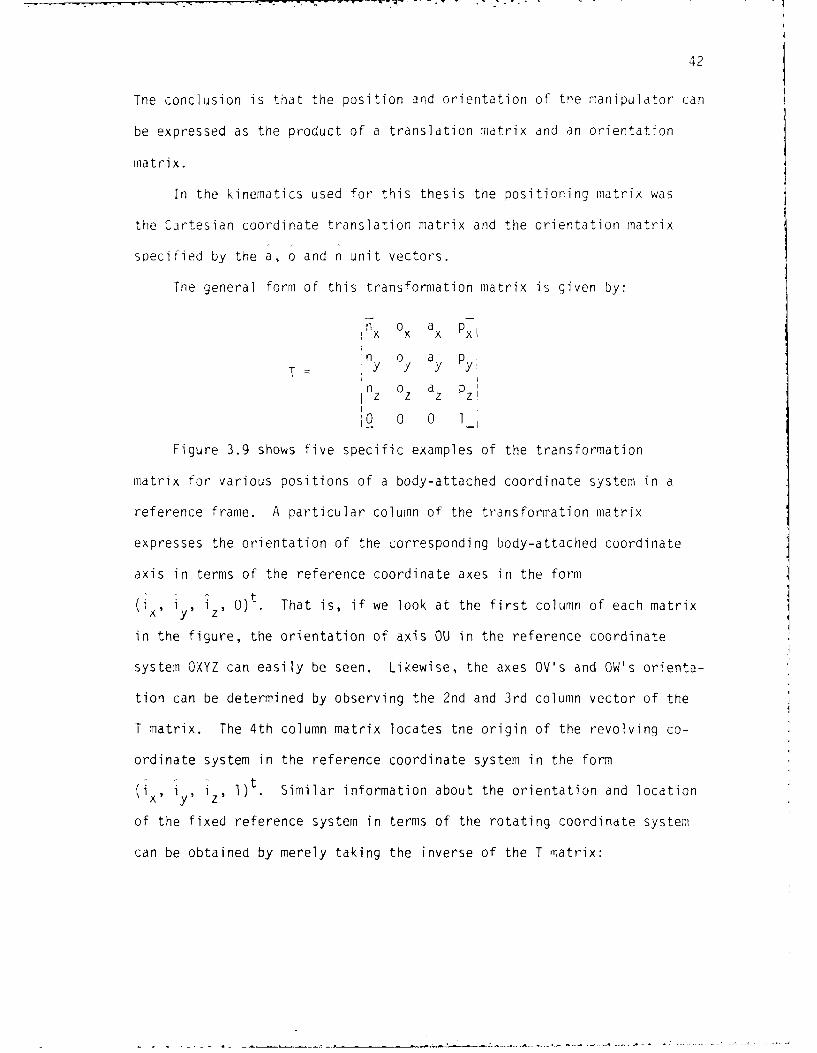
Figure 3.9 Pure Rotation and Translation Matrices

42

The conclusion is that the position and orientation of the manipulator can

be expressed as the product of a translation matrix and an orientation

matrix.

In the kinematics used for this thesis the positioning matrix was

the Cartesian coordinate translation matrix and the orientation matrix

specified by the a, o and n unit vectors.

The general form of this transformation matrix is given by:

nx oX ax Px

n o a pT= Y Y y Y

nz 0z az Pz

0 0 0 1

Figure 3.9 shows five specific examples of the transformation

matrix for various positions of a body-attached coordinate system in a

reference frame. A particular column of the transformation matrix

expresses the orientation of the corresponding body-attached coordinate

axis in terms of the reference coordinate axes in the form

(ix, y, I z 0) t . That is, if we look at the first column of each matrix

in the figure, the orientation of axis OU in the reference coordinate

system OXYZ can easily be seen. Likewise, the axes OV's and OW's orienta-

tion can be determined by observing the 2nd and 3rd column vector of the

T matrix. The 4th column matrix locates the origin of the revolving co-

ordinate system in the reference coordinate system in the form

t(i Iy, i z , ) . Similar information about the orientation and location

of the fixed reference system in terms of the rotating coordinate system

can be obtained by merely taking the inverse of the T matrix:

41

Tbout the z axis and finally a translation z along the z axis. Therefore

tie matrix representing such a position is given by:

Cyl (z,,r) Trans (O,O,z) Rot(z,..) Trans (r,O,O)

z a

zn

Y:yr

x

Figure 3.7 Cylindrical Polar Coordinates [Paul, 1981]

In Figure 3.3 the specification through spherical coordinates, r, , and

corresponds to a translation r along the z axis, followed by a rotation

about the y axis and finally a rotation , about the z axis. In this

case tne position can be described as:

Sph ( ,.,r) = Rot (z,,) Rot (y,.-) Trans (O,O,r)

a

z

r

y

r Ix

igu're 3., Spherical Polar Coordinates [Paul, 1981]

40

Euler (;,., ) = Rot(z,,) Rot(y,i) Rot(z,.,)

The third method for expressing the orientation of the end-effector

is given in terms of the roll, pitch, and yaw angles, terms commonly

used in speaking about ships. Figure 3.6 depicts the situation corres-

z

ROLL

YYAW -pYAW PITCH

X

Fiqure 3.6 Roll, Pitch, and Yaw Coordinates for a Manipulator

ponding to a rotation : about the z axis (roll), then a rotation - about

the y axis (pitch) and a rotation ., about the x axis (yaw). The general

rotation matrix is given as:

RPY(:,, ) = Rot(z,s) Rot(y,.) Rot (x,,,)

In addition to specifying the orientation of the coordinate frame

of the end-effector, a position for the origin of this frame must be

established. In the first method a vector p was introduced to specify

this position in the base coordinates. This position can also be de-

scribed in both cylindrical coordinates and spherical coordinates. In

Figure 3.7 the specification through cylindrical coordinates r, .,, and z

corresponds to a translation r along the x axis, followed by a rotation

39

z

x

z z

XI J

ZI I

yI

Figure 3.5 Euler Angles

0 38

The orientation and position of this hand can be described by an

attached coordinate frame whose origin is located at the midpoint between

the two fingers. This origin is also described by a vector p whose co-

ordinates are expressed in the defining reference frame. There are three

unit vectors which describe the orientation of the hand. The approach.

vector, a, is defined as the direction from which the hand would approach

an object. The orientation vector, o, is in the direction specifying the

orientation of the hand, from fingertip to fingertip. The normal vector,

n, will complete the right handed coordinate system and is specified by

crossing the o vector into the a vector [Paul, 1981].

There are a number of ways of specifying the orientation of a

manipulator or in this case the end-effector. It is obvious that within

the general matrix there are only a few values that afford any information.

r7, For example the bottom row will be tnree zeros ind a one depending on

whether scaling and perspective become involved.

The first method presented in the text [Paul, 1931] is by specifying

the three vectors a, o and n discussed before. These three vectors

specify the orientation of a coordinate frame whose position can be de-

fined in a number of ways to be discussed later. The constraints on this

method are simply that the a, o and n vectors are of unit magnitude, and

the p vector describes a location that can be reached by the manipulator.

The first method can be viewed as a Cartesian approach because orient-

ation is expressed as distances along these three axes. The second and

third methods are expressed as a set of rotations. The second method,

using a set of Euler angles, can describe any orientation in terms of a

rotation ;about the z axis, then a rotation -, about the new y axis y',

and finally a rotation ,about the new z axis z" [Figure 3.5]. In this

case the general rotation matrix car be expressed as:

37

T 0 0 dx

0 1 0 dyT =tran 0 0 1 dz

0 0 0 1_

In deriving kinematics equations for any robot the main consider-

ation is that of orienting and positioning the end-effector of the robot.

For the purposes of this thesis the end-effector is the fifth link of

the robotic manipulator. Therefore in specifying the individual elements

of the general transformation matrix 0T much more information is establish-

ed than merely transforming the coordinates of a vector expressed in the

final link's coordinate system into the base coordinates.

One method of interpreting the general matrix is by specifying three

vectors n, o, and a as shown in Figure 3.4, which represents the end

effector of a robot.

n

p a

Figure 3.4 Orientation Vectors Associated with Manipulator [Paul, 1981]

36

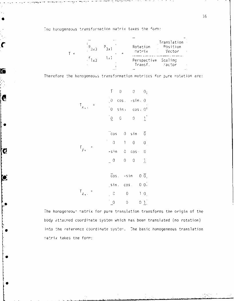
The homogeneous transformation matrix takes the form:

Translation

R P Rotation PositionT ximatrix Vector

lx3 lPerspective ScalingTransf. Factor

Therefore the homogeneous transformation matrices for pure rotation are:

70 00

0 cos, -sin, 0T

0 sin, cos, W

0 0 0 1

cos 0 sin

0 1 0 0'

TY, -sin 0 cos 0

0 0 0 1

cos, -sin 0

sin. cos, 0 0

Tz,. 0 0 1 0

0 0 0 1

The homogeneou- matrix for pure translation transforms the origin of the

body attached coordinate system which has been translated (no rotation)

into the reterence coordinate system. The basic homogeneous translation

matrix takes the form:

0

0

35

an angle = 90'. This transformation can be expressed as:

Pxyz = Rx,: Puvw

Therefore this rotational matrix can be expressed as:

i i ixj i *k w 1 0 0Ix U Xv X Wi

Rx_ jy'i Jyj jy k = 0 cosa -sin u y V y w

kzi k j kz'k 0 sina cos)

Similarly for rotations about the axes OY and OZ we can find rotation

matrices Ry and R respectively. These can be expressed as

cos: 0 sin cos. -sin 0

R = 0 1 0 I R sin. cos., 0y Z,sin.j 0 cos 1j 0 0 1

By knowing these 3x3 matrices we can decompose complex rotations into

their basic rotation matrices and derive the complex rotational matrix R.

R=R *R *Rx,. y, z,'v

By adding an additional coordinate to the position vector

Pxyz = (wpx, WPy, wp ,W)t

the position of the point is expressed in homogeneous coordinates. As a

result, the 4x4 homogeneous transformation matrix now has the capability

of expressing coordinate system rotation, translation, scaling, and per-

spective. The homogeneous matrix is composed of the original rotation

matrix in addition to 3 new components:

- 3xl position vector

- 1x3 perspective vector

- lxl scaling factor

34

z

0: 90C,

rV

Figure 3.3 Rotation of the Body Attached Frame

PX = 1X'PUVW = ixi uPu + ix'jvpv + ixk wPw

Py = ' Puvw = iuPu + j y*jvPv + j ykwPw

Pz = iz'Puvw = kz.i u Pu + kz'jv pv + kz'kwPw

These three equations can be expressed in matrix form:

p ix'l i j i k Px = yu xv x W up i j*j j *kz Y, u y v Y v

and so the transformation matrix A that relates the body attached coordi-

nate system to the reference coordinate system has been determined.

Likewise there exist a 3x3 matrix B that transforms a vector in the OXYZ

coordinate system into the OUVW coordinate system:

Puvw xyz0

Since any complex rotation can be divided into three component

rotations, the next step in developing the forward kinematics is to

derive the basic rotation matrices for rotation about the three axes

of the reference frame. Figure 3.3 shows a rotation about the OX axis by

33

Fz

Figure 3.2 Body Attached Coordinate Frame and Reference Frame

Obviously point p can be specified in either of the coordinate

systems, that is:

Puvw = (Pu'pv'pw)t

Pxyz = (PxPylPz t

If the block is rotated by some arbitrary angle, the point p, which

is fixed to the block, is also rotated [Figure 3.3]. That is, the vector

(pxPypz)t has changed while the vector (pu,PvPw)t has remained

constant.

A rotation matrix (3x3) can be constructed that maps the co-

K0 ordinates of a position vector in a rotated coordinate system (OUVW) in-

to a reference coordinate system (OXYZ) [Lee, 1982]. Therefore the

vector p =p + p I + w when projected onto the coordinate

frame OXYZ axes, will yield:

0i ii l i =iii 'i

32

In order to perform even the smallest movement of a robotic arm

(manipulator), there must be specific changes in the angles or displace-

wents that exist between the set of links and joints. The manipulator's

position and orientation in space may be specified by examining the

position, orientation, and dimensions of each link.

The kinematics problem is generally divided into two parts:

- forward kinematics is concerned with the position

and orientation of the manipulator given a set of

joint angles.

- inverse kinematics is concerned wic:h deriving a

legitimate set of joint angles given a position

and orientation of the end-effector of a robot in

some reference coordinate system.

Forward Kinematics

In viewing the forward kinematics problem it is necessary to in-

vestigate the relationship between a stationary or reference frame and

a coordinate system that is able to revolve and/or translate. Lee [Lee,

1982] discusses this topic using a rigid body example, where there is a

body-attached coordinate frame on a block located in a reference co-

ordinate system [Figure 3.2].

In this figure we have two right-handed rectangular coordinate

systems. OUVW is a body-attached coordinate system that will change

position and orientation as the rigid-body does so. OXYZ, on the other

hand, is a fixed reference frame. The purpose here is to develop a given

transformation matrix from the OUVW coordinate system to the OXYZ

coordinate system.

CHAPTER III

ROBOTIC MANIPULATOR KINEMATICS

In this chapter robot configurations and kinematics are reviewed and

a description is given of the specific robot manipulator used in this

study and of the computer network providing control for that manipulator.

Then a description of the system equations used in the particular

estimation problem which illustrates the integration of the vision

acquisition system with the mechanical manipulator arm is presented.

Kinematics is basically a description of the geometries associated

with a mechanical system. Many industrial robots of today consist of N+l

rigid bodies called links and N connections known as joints. There are

two types of joints, translational and revolute, whose names indicate the

types of motions the joints perform [Figure 3.1].

TRANSLATIONAL JREVOLUTE

Figure 3.1 Two Types of Robotic Joints

31

30

Xlength.

initial boundary II search in X direct l--1 ILc -

IfYc Ylength

"result: X S initial Y center searchc c

secondary Y center

searches

secondary XC center searche

*i Figure 2.13 Cross Hairs Method

I

-I ., - _,.. .. .,.... . .. . .. . . .. . . . . . .'

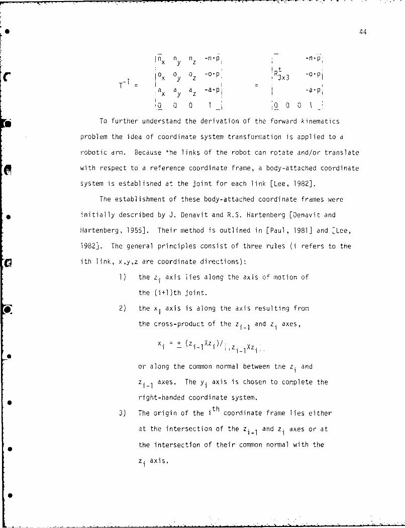
44

,x ynz --a n y -on.p

Rt

-ox 0y 0z o.p 3x3 o plT T a~ a a -a-p -a-

x y z-ap

0 0 0 1 ,0 0 0 1

To further understand the derivation of the forward kinematics

problem the idea of coordinate system transformation is applied to a

robotic arm. Because +he links of the robot can rotate and/or translate

with respect to a reference coordinate frame, a body-attached coordinate

system is established at the joint for each link [Lee, 1982].

The establishment of these body-attached coordinate frames were

initially described by J. Denavit and R.S. Hartenberg [Denavit and

Hartenberg, 1955]. Their method is outlined in [Paul, 1981] and [Lee,

1982]. The general principles consist of three rules (i refers to the

ith link, x,y,z are coordinate directions):

1) the z, axis lies along the axis of motion of

the (i+l)th joint.

2) the xi axis is along the axis resulting from

the cross-product of the zi-l and z. axes,

xi + (zi_ XZi)/: zi Xzi i

or along the common normal between the zi and

zi-i axes. The Yi axis is chosen to complete the

right-handed coordinate system.

3) The origin of the ith coordinate frame lies eitherat the intersection of the zi- l and zi axes or at

the intersection of their common normal with the

zi axis.

0

Denaivit and Hartenberg also present four additional quantities

that completely describe any revolute or translotional joint. It is

important to recognize that the links maintain a fixed relationship

between the joints [Paul, 1981]. The four parameters are:

the joint angle from, the xiI axis to the

xi axis about the zi 1 axis

dI• the distance from the origin of the (i-l)th

coordinate frame to the intersection of zi-1

axis with the xi axis along the z. axis.

a. the offset distance from the intersection of

the z i1 axis with the xi axis to the

origin of the ith system along the xi axis (or

the shortest distance between the z il and zi

axes).

i the offset angle from the z,-1 axis to the zi

axis about the xi axis (using the right-hand

rule) [Lee, 1982].

Depending on the type of joint some of the quantities are constants.

That is, for a revolute joint the values of di , ai and ,i remain constant.

Since i changes, it is given the term "joint variable." While with a

translational joint the values of ai , -'i and are constant and di

becomes the joint variable [Figure 3.10].

Once the coordinate system for each link has been established, a

homogeneous transformation matrix relating the coordinate system of link

i to that of link (i-l) can be found. That is, the orientation of the

ith coordinate system in the (i-l)th system can be reduced to four basic

transformations:

0 . .• _ . . • . .. .: . .. ... ...... ..... .. ...i ...

46

Link i

II iY zi-

it ia i

x i

d i -I'

-_ _ -

Link i-I X

Figure 3.10 Joint Variables and Quantities

1) rotation about zi axis an angle i to align the xi

axis with xi axis,

2) translation along the z i_ axis a distance d. so that

x il and xi become coincident.

3) translation along the xi axis d distance a. to

bring the origin of both coordinate systems into

coincidence.

4) rotation about the x i axis an angle .i so that

z i-I axis and zi axis are aligned.

As a result the homogeneous transformation matrix relating any ith

coordinate system to the (i-l)th coordinate system would be the matrix

product of these four basic transformations:

0

47

A =T T T TI- z, zd x,a x,4

For revolute joints, the resulting matrix takes the form

cos- -cosaisin. i sinisi n. aicos.

sin-Ci COs:icos i -sinticos. i aisin i

0 sin,. cos-. d.1 1 l

0 0 0 1

and for translational joints, it becomes

cos.,i -cos~isi n-.i si nisin, i

s1n-: i cosai cos., -sin ,(icosvi 0

0 sin-i cosi di

_0 0 0

Forward Kinematic for P-5 Robot

The robot used in this thesis research was the General Electric P-5

process robot. A graphical depiction of the robot can be found in Figure

3.1. Using the Denavit and Hartenburg method for establishing co-

ordinate frames, and both Paul and Lee's descriptions on how the homo-

geneous matrix between joints and coordinate frames can be established,

the following description of the forward kinematics of the P-5 was

arrived at.

S48

a(3

2 a2 ,5z 1d

24

0 X YO

Figure 3.11 Five Link Robot Similar to the P-5 Process Robot

In Table 3.1 the necessary link parameters of the P-5 process robot are

tabulated.

( Table 3.1 P-5 Robot Joint Parameters

HomeJon Constant parametersJoint Position

Link variable . a J d

* 1 00 0 900 65cm

2 900 60cm 00 0

'390 80cm 0 ° 0

- 4 - 900 0 900 0

5 5 00 0 00° 0cm

In order to establish the position of a point in coordinate system

i referred to the base coordinate system we must develop the homogeneous

transformation matrix 0Ti. This is given by the product of the individual

transformation matrices AI A 2 Ai

49

The matrix A as was stated in the previous section is a specific

application of the general matrix Al whose form was given previously.

For the P-5 robot with the notation Cos2.i Ci and Sin. Si , the in-

dividual A matrices take the form: jC1 0 S1 0

I S 0 -C 0 d = 65 cm a =0.0 cmAO=

0 1 0 dl 90

0 0 0 1

C 2 0 a2C2

I2

S2 C2 0 a2S2i d2 = 00 a2 = 60 cm

A 0 0 1 01 = 00! -L2

0 0 0 1_

C3 -S3 0 a3C3

S3 C3 0 a3S3 d 0 cm a3 = 80 cm

2 0 0 1 0 0

0 0 0 1

C 0 S 0,'4 44 4 0 C4 0i d 0 cm a4 = 0 cm

A3 - 0 1 0 01. 900

Sl4

5 -$5 0 0-1

IS5 C5 0010 - cm a = 0 cm

4 =

0 0 1 d5 ! A = 0 °

0 0 0 l-

Now the coordinates of any link relative to some reference coordinate

frame can be expressed as an appropriate product of these matrices.

. L. . . . . . i -1 . .i ' - .....:,...-,..,',..o-.., _, , L -._ . SI

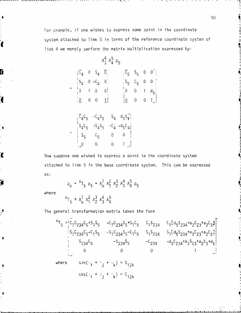
50

For example, if one wishes to express some point in the coordinate

system attached to link 5 in terms of the reference coordinate system of

link 4 we merely perform the matrix multiplication expressed by:

A4 A5 IS 4 0 S 4 0' S C5 0 0$4 0 -C 0 $50 0 0

S0 1 0 0: 0 0 1 d5

0 0 0 l 0 0 0 1

$405 -$4S5 -C4 -d5C4

S5 C5 0 05 51

_0 0 0 1_

Now suppose one wished to express a point in the coordinate system

attached to link 5 in the base coordinate system. This can be expressed

as:

0 T5 p A1 A2 A3 A4 A5 pTo :°5 P5 = A

where

T A1 A2 A3 A4 A55 01 23 4

The general transformation matrix takes the form

°T5 I1CIC 2 3 4C5+S1 S5 -C1C2 34 S5 +SIC 5 C1S23 4 C1 [d5S 23 4+a3C2 3+a2C21T

SIC 2 34C5 -CIS 5 -SIC 23 4S5-CIC 5 SIS234 Sl[d 5S2 3 4+a3C23 +a2 C2]

S C -S S -C -d C +a S +a S+dI234C5 234S5 234 5C234 3S23 2S3 1

0 0 0 1-

where sin(,; i + + k) Sij k

cos( i + + -:.k) ijk

51

Therefore with the general matrix transformation 0T5 any position of the

end effector expressed in the fifth coordinate system can easily be

transformed to base coordinates.

Inverse Kinematics

The inverse kinematic's problem may '5e the more important problem

in this discussion. The reason for this is simply that most robotic

arms or manipulators are positioned and oriented by a combination of

joint angles. This gives imnortance to the ability to transform real

world coordinates into this particular set of joint angles. "Obtaining a

solution for the joint coordinates requires intuition and is the most

difficult problem we will encounter ..." [Paul, 1981].

Paul presents a general approach to the solution along with some

problems that may be avoided. He also suggests that since the end

effector of an n-link manipulator has a general transformation matrix

SA 1 A2 . An- I Ann A0 n-2 n-1

by simply recursively premultiplying the matrix by the inverse of a link

transformation the specifications for the necessary joint angles can be

obtained. To facilitate understanding of the technique it will help to

introduce Paul's discussion of Euler angles and their solution [Paul, 1981].

Euler angles can describe any possible orientation of the end

effector in terms of a rotation t about the z axis, then a rotation

about the new y axis y' and finally a rotation -, about the new z axis z".

As previously discussed, the orientation of the end effector can be

expressed as a product of 3 rotation matrices which becomes:

52

cos;cos;cossin:sin, - coscos:sin - sin:cos,

sinsinsin + cos-sin, - sin.cossin. + coscosyEuler (:,)l

-sinjcos si n..sin,,

- 0 0

cos..sin7,

sin:sin: 01

cos" 0

0

Since this should yield the homogeneous transformation matrix that was

presented in the previous discussion, it must be true that:

In o a

Euler (;,:,>) = ny 0 a py y y y

n o a Pznz z z Z

o 0 0 1_

As a result, the unknown Euler angles should be determinable from this

matrix equation. The obvious solutions from these equalities are:

= cos- (az)

cos- (ax/sin-)

= cos- (-n /sin,,)z

As Paul points out there are several problems with this approach.

1) In using the arc cosine function:

a) the sign is undefined

b) the accuracy in determining the angle itself is dependent

on the angle

I

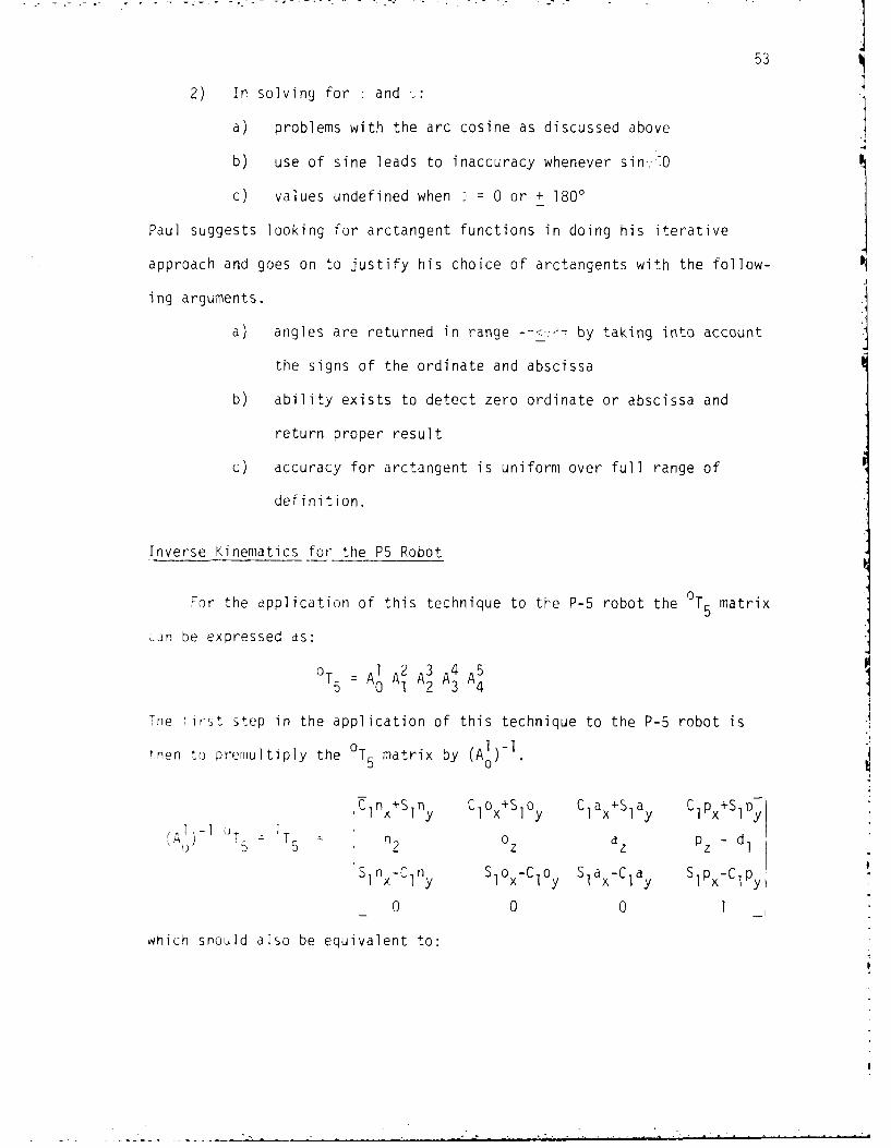
I2) In solving for and

53

a) problems with the arc cosine as discussed above

b) use of sine leads to inaccuracy whenever sinv7O

c) values undefined when -, = 0 or + 1800

Paul suggests looking for arctangent functions in doing his iterative

approach and goes on to justify his choice of arctangents with the follow-

ing arguments.

a) angles are returned in range --<.z-- by taking into account

the signs of the ordinate and abscissa

b) ability exists to detect zero ordinate or abscissa and

return proper result

c) accuracy for arctangent is uniform over full range of

definition.

Inverse Kinematics for the P5 Robot

For the application of this technique to the P-5 robot the 0T5 matrix

,-,n be expressed as:

0 4 A

The *irst step in the application of this technique to the P-5 robot is

then to premultiply the T5 matrix by (A0 )-

Clnx+Slny Cl 0x+S 0y Cla+S ay ClPx+SlP1 n y a p - d

,A T 5 T5 n2 0z az z d

S1 nx-Clny SlOx-Cl0y Slax-Clay SlPx-ClPy

0 0 0 1

which should also be equivalent to:

54

C234C5 -C234S5 S234 d5S234+a3C23+a2C2

s234C5 -S234S5 -C234 -d5C234+a3S23+a2S35 S5 C5 0 0

0 0 0 1

To be equivalent each term of the matrix must be equdl to the corresponding

term. By equating the third elements of columm four, I can be found:

Sl~x C~l~y = 0

tan-1 x

= tan - iyI Px

The next angle of interest is 5" By equating the third elements of the

Ist and 2nd columns 5 can be found:

S5 -- Sl nx - C ny

C5 = S1Ox - Cly

S - Cn I

5 x tan S 0 1 0 Next can be determined by equatingi *l1x C I Y23

the Ist and 2nd elements of the third columns.

S234 = CIax + Slay

-C 234 a

-1 ir(-C Ia -

~24=tan a234 z

The solutions for :2':3":4 can be found using a trigonometric technique.

After equating appropriate terms the identities of interest are:

C1px + SlPy = S234d5 + C23a3 + C2a2

Pz- dl = -C2 3 4d5 + C23a3 + S2a2

55

By manipulating the equations and defining two intermediate values it

can be shown that: I

q = CP x + SIPy - S2 3 4d5 = C2 3a3 + C2a 2

r p pz-d I + C234d5 S 23a3 + S2a2

q2 C 2a2 + 2C2C23a2a3 + C2a 22= $ 3 a + 2S2S23 a2a3 + Sa,

2~ r2 2+ 2 C2 + $2 22(C 3 a + 2~ 3 ) a a C + S

q(23 S23)a3 2 3(C2C23 s2S23) a2 2 2

= a 2+ 2a2a3(C 2C23 + $2S23 ) + a2

Now by examining the middle term, it can be shown that:

C2C23 + $2S23 = cos(V 23-.2 ) cos 3 = C3

2 r2 2 2q 23 + a2 + 2a2a303

2 r2 2 2q 2+ r2_ a- a 2q 3 2C3 = 2aa 3

S + V, 1 - C 2 yields 2 values3 -l 3

3= tan- (S3 /C3 )

q = C23a3 + C2a2 = C2C3a3 - S2S3a3 + C2a2

r S23a3 + S2A2 = S2C3a3 + C2S3a3 + S2a2

q S2 (-S3a3 ) + C2 (C3a3 + a2 )

S 2 (C3a3 + a2 ) + C2 (S3a3 )

Cramer's rule is then exployed in finding solutions for S2 and C2:

2 2

-S3a 3 C3a 3 + a2

C~a2 2 2 2= S3a3 (C3 a3 + a2)

C3 a3 +a2 S3 a3 j2 2 _ 2 2 2

-S3a3 LC3a3 + 2a3C3a2 + a2]

= -a3 2a2 a3 C3 - a2

3 2 33 2-(a3 + 2C3a2 a3 + a2)

q C3 a 3 + a.

S = qS3a3 - r(C3a3 + a2)

,r 3S3a3

S2 qS3a3 - r(C3 a3 + a2)2 2

-(a3 + 2C3a2a3 +a2 )

-S 3 a3 q

C2 -rS3a3 - q(C3 a3 + a.)

iC3a3+a2 r,

C (r)3a3 + q(C3a3 + a2 ))

2 2 2-(a 3 + 2C3a2a3+a2 )

2 tan- (n2)22

234= 2 + 3 + 4

4 234 2 3

the vector of joint angles is thus determined.

Aithin the working system there are two added constraints that have

an effect on the specific form of the 0T5 matrix. The first is the task

57

of .iaintaining the orientation of the fifth link parallel to the floor.

It can be accomplished by properly selecting the vectors a, o, and n,

which were discussed previously. The set of equations that specify this

task is:

Px-- -- = n = 0

ip x y

p-- = n = -o x

0.0 = nz =0O.=n o

The second constraint is that the manipulator is maintained at a fixed

height when not in motion. This constraint is realized by passing a

constant value for the z parameter to the controller.

Calibration of Camera to Robot

In this project an additional transformation is due to the introduction

of the camera into the system. The camera's image field acts as another

coordinate frame. As a result of the restrictions in link 5 and the fact

that the camera is mounted to a fixed frame [Figure 3.12], the camera lens

is maintained parallel to the floor. Therefore, this transformation is

only necessary in two dimensions.

Figure 3.12 P-5 Robot, Vidicon Camera, Laser

71

deviation are relatively of the same size in the range .5 -1.5 for the x

and y coordinate and also the radial distance.

The next significant source of error was that due to the repeat-

ability of robot motion. That is, what is the standard deviation of the

error between a desired position and the actual position, when the robot

is repeatedly asked to go to the desired position. In this test the robot

was started at the home position. The image of a stationary object was

used to direct a motion of the robot. When the move was completed, a new

image of the object was taken, and the coordinates of its center were

determined. The results of 100 such trials were:

x = 1.98

y= 6.12

r = 35

In each case an average value was determined. Then, using this

value as the mean, a variance and standard deviation were calculated . TIn

this experiment it is obvious that the repeatability of a move is different

in the x and y direction. Because these standard deviations are expressed

in pixels the true deviation of the repeated position is rather small. How-

ever these pixel values provide a basis for evaluating the overall system

error. Without any estimation taking place these values give an indication

of how accurately the robot can be placed over a stationary object. It

is obvious that in the overall system the fact that a moving object is

used and an estimation is attempted should yield higher expected standard

deviations.

The time constraint on the minimum estimation time is influenced

by two specific times. One was the time used to calculate the object's

estimated position, and the second was the time period between the be-

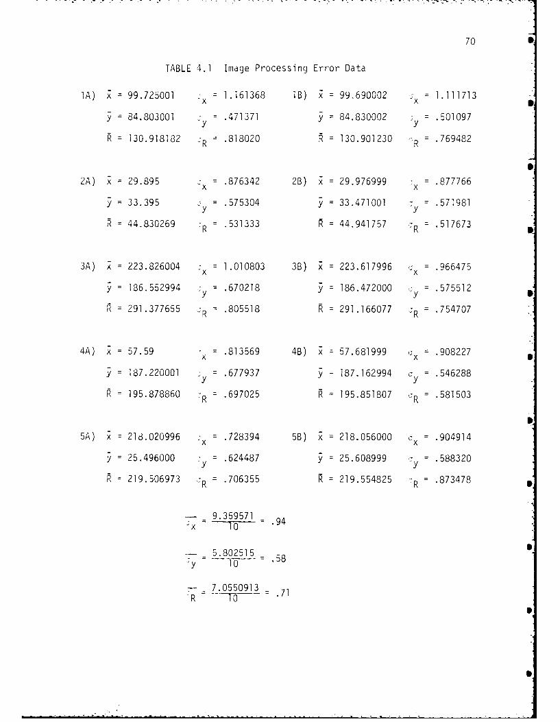
70 S

TABLE 4.1 Image Processing Error Data

A) x = 99.725001 x= 1.161368 IB) x = 99,690002 :x = 1.111713I9 0

y = 84.803001 - = .471371 y = 84.830002 y = .501097

= 130.918182 .R = ,818020 R = 130.901230 .R = .769482

2A) x = 29.895 x = .876342 2B) x = 29.976999 -x = .877766

y = 33.395 = .575304 y = 33.471001 = .571981Y Y

= 44.830269 :R = .531333 = 44.941757 R = .517673

3A) x = 223.826004 -x = 1.010803 3B) x = 223.617996 -jx = .966475

y = 186.552994 y= .670218 y = 186.472000 7y = .575512

= 291.377655 .R = .805518 R= 291.166077 j = 754707

4A) x = 57.59 x .813569 4B) x = 57.681999 x .908227

= 187.220001 : = .677937 y z 187.162994 = .546288

= 195.878860 R = .697025 R = 195.851807 o R = .581503

5A) x = 218.020996 :x = .728394 5B) x = 218.056000 ox = .904914

y= 25.496000 y = .624487 y = 25.608999 = .588320

= 219.506973 .R = .706355 R = 219.554825 R = .873478

9.359571x 10.9

5.802515 q'Y 10 .58

- 7.0550913 7- .71"R 10

S

69

deviation from this average value was derived. The data derived in the

experiment is presented in Table 4.1. The data in this table represents

experiments performed at five locations within a zoomed image field.

These five locations, labelled I through 5 in the table, include the four

corners and the center of the zoomed image field in order to detect any

variations over the field. Each position is represented by two experi-

ments (A and B). Each block of experimental results consist of the average

object center x coordinate and y coordinate. The average radial distance

from the image field origin, and the corresponding standard deviations.

In addition, the table includes a list of the average standard deviations

over all data.

The data in the table reveals some interesting features about the 1

image acquisition system for the static case. The most obvious result

is that the standard deviation in the y direction is consistently lower

then that of the x direction. At this time there is no obvious reason

for this type of bias. Another interesting result that is evident is

that the standard deviations of the x and y coordinates and radial

distance are on the average less than 1.0 pixel. The data in this experi-

ment typifies the actual data received in the working system. That is the

zooming feature of the imaging system has been incorporated so that

results of data acquisition within the tracking experiment would be con-

sistent with the data provided here. This simply means that even with the

reduced resolution of the object in a zoomed mode the variance from the

mean would be less then a pixel in the static case. The third interesting

feature revealed by this experiment is that no area of the camera field

reveals any true deviation from value of other areas. That is the standard

68

The dynamics of the P-5 robot seem to be the major source of error.

When the robot is directed to proceed to a position, although there is aS

form of velocity control, it is obvious that overshoot occurs and vibration

is present at the conclusion of the move. This vibration may cause slight

snifting of the camera or mispositioning of the robot. Both of these

problems would result in errors for the image processing application. An-

other problem introduced by the P-5 robot that may cause inaccuracies in

the calculations or even in the actual positioning is the repeatability ofS

the robot. That is, given a position command how accurately can the robot

repeat this position?

There are additional considerations which must be taken into account.

For example, throughout the research the presence of noise in the image

field has been observed. This source of error influenced the choice of

the center finding technique as discussed previously. Furthermore, com-

putational and mechanical movement times put limits on the minimum pre-

diction time.

The first source of error of interest is that introduced by the

image aquisition system. As was stated previously, the main task of this

system is to determine the value for the center of the object that is

being tracked. This does not have to be the true centroid, however

the value that is determined should be repeatable to some degree of

accuracy even in a "noisy" environment. The test to discover the error

in this measurement was a static test. Although the motor power to the

robot was on, there was no directed movement during the test. The pro-

cess consisted of placing an object at several locations in the image

field and making 1000 measurements at each position. For each position

an average x,y, and (x2 + y2)I/2 value was deterr, ined and a standard

CHAPTER IV

EXPERIMENTAL RESULTS AND ANALYSIS

In this chapter a number of experiments and their results used to

evaluate the performance of the "intelligent robot" system are pre-

sented. At the conclusion of the chapter a Kalman filter model of a

linear estimator is given in order to have a basis for evaluating the

experimental results obtained.

In order to facilitate the analysis of the data recorded in this

research, it will be important to understand in general what the specific 0

sources of errors are. To this end an attempt was made to examine all

the contributions to the overall error in terms of camera pixels.

Experiments and Results

The system as described in the previous chapter contains a number of

devices that may cause the introduction of errors into the system. 0

Although the software has tried to compensate for image acquisition errors

there are a number of possibilities that may arise that could raise the

probability of inaccuracies in the image gathering technique. For 0

example, if the robot is vibrating or moving in any way while the images

are being taken each image will not be taken at the exact same location.

Even in the static case the software may not derive the same center of the

object each time due to noise or slight rotation of the object. The

improper illumination of the object field may also cause the center of the

object to shift.

67

66

in addition to this estimation routine for the moving object there

is a process in the software that attempts to avoid possible indications

of false velocity. If the object is stationary an error in the center

finding routine nay indicate a change of position and therefore a velocity

that is not truly present. As a result, depending on the estimation

period, the robot may be directed to an erroneous position. To avoid this

problem the software observes very small changes in positions as such, and

directs the robot to remain at the present position for a specific sampling

period. By storing the robot's previous position in this process a "catch

up" maneuver can be made when the object has definitely traversed a

specific distance. As a result there may be several sampling periods

when the object is moving slowly enough to warrant the robotic manipulator

to remain in place. However, even with very slow movement, over a period

of time a large enough distance will have been traveled so that the

manipulation must be moved just to catch up to the object.

65

one having xI as the initial position, the other having x2 as the initial

position. In a similar manner the estimated position Y3 is found. The

equations are:

x= 2 (X1 + 2XlT + x + XLT)

Y3= T (y + 2Yl.T + Y2 + Yl T )

Then error terms in x and y are formed using the actual x3 and Y3

values obtained from the third image:

err 3 3

Yerr Y3 Y3

Finally, the estimates x4 and Y4 are found as a combination of the average

estimates resulting from using the coordinate positions of the three p

images as separate initial conditions and appropriate velocities and times

plus a contribution proportional to the error term. The necessary

equations are

x4 (Xl + ),LT + a + T + x T + x3 + T)avg 122 2 T+ v avg

+ XerrT/T

Y 3 + (Y+ 2 )T + YavgT + Y2 + Y2i T + Yavg + Y3 + avgT)

+ YerrT/LT.

The predicted position x4 at T seconds after acquisition of image

three is the sum of four terms. The first term is the x4 coordinate

estimate using xI as the initial position and using velocities I and 2

and their respective T's and velocity x + x2/2 = x and time T. The1 2 avg

second and third terms are similar to the first but with initial positions

x2 and x3 and using velocities x2 and X avg" These three terms are averaged

and the fourth term represents an error that is linear with time. The y

equation follows in a similar manner.

I

. . 4, -- -4.- , . -- .o- -. . . . . . -. . . . - -. • . - o- - - . . . . .w - - - ,i . v ,.- - ' ,

64

0 4T, Y T i,Y T = estimation

position time

x4,y 4

Xerr

Y3

y2

x1 x2 x3 c x

Ii (x 2- xI)/,dT 1= (Y2-Yl)/6 T

2 (x 3-x2)/2T 2: (Y '

avg=( 1+t2)/2 avg= (1 +-

A

Xerr X 3- x3 yAeerr: Y3-Y3

Figure 3.14 Estimation Technique

of this data, velocities x and yl are then calculated. Using this in-

formation, an estimate of the objects position in image three is made.

The estimated position x3 is found from the average of two predictions,

* 63

several object images whose temporal relationships are know. The in-

formation gained through this sequence of images allows estimation of

C object position at a future time. The limits on the specific estimation

time period are governed by two considerations. First, the time required

for image acquisition, image processing, estimate calculation, coordinate

transformations, and response time of the actual manipulator movement

determine the minimum estimation time. Secondly, the accuracy of the

estimated position, which decreases as the estimation period increases,

and the size of the camera image field, which limits the maximum

position error allowed, determine the maximum estimation time that will

insure that the object is in the field of view.

The demonstration example which is used to illustrate the ideas

of this thesis consists of estimating the position of a moving object

based on information from a sequence of three images. Figure 3.14

C7 shows the space and time relationships in the estimation technique used.

This is also performed as a software function. That is, as the program

proceeds, the encoder counters are compared to the desired values. This

All set of differences is used to determine the velocities of the correspond-

ing links. The method sets a joint's velocity at a fraction of the

maximum velocity equal to the ratio of its encoder count difference

S to the maximum count difference over all five joints. This approach is

applied repetitively as the move progresses, thereby providing closed-

loop control.

The equations used attempt to take into account all information at

each step for the purpose of minimizing large errors in any one

measurement. The technique initially takes three images _'T apart in

time and finds their centers (x ,y1),(x2,y2) and (x 3'Y3) On the basis

62

two control loops. The first is a tachometer-controlled loop which

produces a so-called "desired" motor current. This signal is compared

then to the actual motor current. The error signal in this loop will

determine the pulse width of a 20 KHz pulse train used to drive the

individual motors of the robot. The purpose of using two control loops

is to account for the nonlinearities of the robot's motors.

The P-5 process robot is electrically driven and is capable of per-

forming a wide variety of industrial tasks. It is a five joint, five link

robot which was initially designed for teaching playback type of operation.

The Estimation Used in Demonstration Task

Recall that in this thesis the main objective is to move the robotic

manipulator in response to some visual information obtained from an image

acquisition system. This visual information may be related to an object

which is either fixed or moving. The ability to extract information such

as object position, shape, size, speed, direction of movement, or even

acceleration, makes possible the handling of a number of industrially re-

lated tasks. Typical tasks include object removal from or placement on

a moving conveyor belt; painting, welding or other operations on a

stationary or moving object; separation of objects based on the results of

a visual inspection performed by the image acquisition and processing

system. Since a number of industrial tasks require some interaction with

moving objects, the ability to track or estimate positions of these

objects is an important element in the operating features of an intelligent

robot. These considerations have led to the selection of moving object

interception as the demonstration example used to illustrate the ideas in-

vestigated in this thesis. This interception problem requires the use of

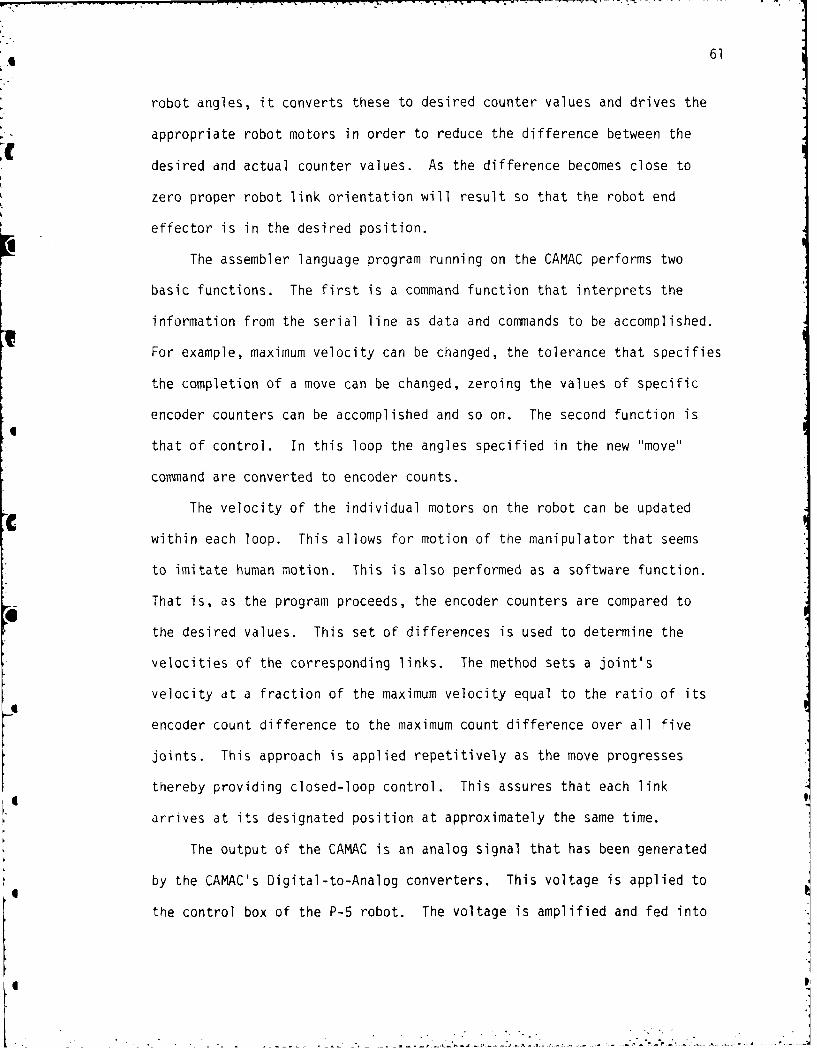
6 61

robot angles, it converts these to desired counter values and drives the

appropriate robot motors in order to reduce the difference between the

desired and actual counter values. As the difference becomes close to

zero proper robot link orientation will result so that the robot end

effector is in the desired position.K The assembler language program running on the CAMAC performs two

basic functions. The first is a command function that interprets the

information from the serial line as data and commands to be accomplished.

For example, maximum velocity can be changed, the tolerance that specifies

the completion of a move can be changed, zeroing the values of specific

encoder counters can be accomplished and so on. The second function is

that of control. In this loop the angles specified in the new "move"

command are converted to encoder counts.

The velocity of the individual motors on the robot can be updated

within each loop. This allows for motion of the manipulator that seems

to imitate human motion. This is also performed as a software function.

That is, as the program proceeds, the encoder counters are compared to

the desired values. This set of differences is used to determine the

velocities of the corresponding links. The method sets a joint's

velocity at a fraction of the maximum velocity equal to the ratio of its

encoder count difference to the maximum count difference over all five

joints. This approach is applied repetitively as the move progresses

thereby providing closed-loop control. This assures that each link

arrives at its designated position at approximately the same time.

The output of the CAMAC is an analog signal that has been generated

by the CAMAC's Digital-to-Analog converters. This voltage is applied to

the control box of the P-5 robot. The voltage is amplified and fed into

",

60

The system is driven by means of a high-level Fortran program run on a

PDP 11/60 digital computer. The program directs the flow of control

from image acquisition, through image processing, to data delivery to a

CAMAC computer.

Following the CAMAC computer an interface has been built to work

with the control box of a P-5 process robot. The interface and control

consist of several pieces of hardware that provide the signals to

operate the motors of each of the links on the robot.

Image acquisition is accomplished through an imaging system develop-

ed by Imaging Technology, Inc. The system, which was disucssed in greater

detail in Chapter II, allows for the acquisition or construction of 2-D

images. The system provides the ability to drive the imaging hardware by

use of high-level languages, such as Fortran and Basic. There are a

number of useful subroutines that allow for a wide variety of processing

applications.

The PDP 11/60 is a digital computer that acts as the main controller

in the overall system. The PDP 11/60 processes the acquired data and

presents the necessary information over a serial line to the CAMAC

computer.

The CAMAC computer is basically a digital computer that acts as an

interface between the digital world of the PDP 11/60 and the analog world

of the P-5 robot's control box.

The CAMAC operation monitors the values held by a group of up-down

counters which record the number of encoder pulses from the corresponding

joint angle encoder of the robot. The values of these counters are a

measure of the appropriate joint angles of the robot and are zero at the

robots "home" position. When the CAMAC computer receives a set of desired

59

the position of the laser. Step four consisted of moving the robot to

several known positions and determining the location of the object in

camera coordinates. After each step the vector that expresses the

position of the end effector in the coordinates of the fifth link is

derived using the equation:

P5 : (T)- p0

As a result a relationship between the camera coordinates and the co-

ordinates of the fifth link can be found. Finally, using a least

squares approach, the A5 matrix transformation is determined [seecam

Appendix A].

Components of the System

A description of the specific hardware and software system under

consideration in this thesis is now given. The system block diagram is

presented in Figure 3.13.

CAMAC CONTROL ROBOT

PDP 11/60,

IMAGING SYSTEM

Figure 3.13 Block Diagram of System

58

The system observes the location of an object in the image field or

camera coordinates pcam* A transformation is necessary to express the5

object's position in link 5 coordinates (A 5a). Obviously, then thecam

position expressed in base coordinates can be given as:

p= To A 5

P0 - T5 cam Pcam

The transformation matrix A5 simply represents a set of equationscam

that take the form of:

x5 axca +by +y5 cxcam yca m X0

Y5 CXcam +dY cam +Yo0

These equations can be expressed in a homogeneous matrix form as:

x a b 0 xo' xcam

5 :c d 0 yo1 c

z5 0 0 1 0 Zc

1 0 0 0 1

The system used in this research did not have a permanently attached

camera. As a result, a calibration of the camera referred to link 5 co-

ordinates had to be accomplished whenever the camera was remounted. The

basic purpose of the calibration was to derive the six unknown constants

of the A 5 matrix.cam

The logical design of the calibration routine was relatively

straight forward. Step one consisted of positioning the robot in a

'home' orientation. Next, a laser which is mounted along with the

camera was used to produce a light image in the camera field. Because

the laser's position is fixed in reference to the camera's position, the

location of the light image in the camera field is also fixed. Step

three was to move the robot to a known position and place an oL, oct under

72ginning of a move and the completion of the move. These two values were

examined by using a system routine that was able to specify the time

4 increments to within 1/60 second. The necessary parts of the program

were repeated and tinied as was the actual movement of the robot. The

experiment was conducted using a wide range of robot motion. After

running through the procedures 1000 times the values obtained were:

AVERAGE TIME FOR CALCULATION =.291 seconds

AVERAGE TIME FOR ROBOT MOVE =.854 seconds

4The data in this section is provided to indicate to the user the

average amount of time needed to process the data in software, derive an

estimate of the object's position, and to actually move the robotic mani-

pulator. The total of these two values will yield the minimum estimation

time that the system can work with. Using a smaller estimation time

would result in the robot's inability to beat the object to the position

eeven if all error was removed trom the system.

In the following section an evaluation of the overall system

accuracy expressed in pixels is given. The experiment for obtaining data

4 to examine the general system consisted of running the system with a minor

software modification. This modification was the addition of a timing

loop that timed out the estimation time using the system clock. At this

point an image was taken and the object's position was examined

The experiment consisted of running this modified program through a

loop 100 times. In the loop the robot started from the home position

each time. At this location the acquisition of three images of a moving

object was accomplished. Using these images, an estimate of the object's

position at a specific time later was determined. The manipulator was

directed to move to this estimated position where it waited for the

system timer to indicate that the estimation period had elapsed. An

image was taken and evaluated to determine the object's new position

compared to the location of the laser in the image field during cali-

£ bration. It is assumed that the laser position can be considered the

system pointer because the initial calibration of the system was per-

formed using the laser image location as a reference point. An error,

expressed in pixels, in both the x and y directions was calculated and

stored. Finally, the robot was directed back to its home position and

the process began again.

After the sequence of loops the error information was used to de-

termine an average error and a standard deviation. The experiment

examined both linear and circular motion using estimation times of three,

* five, seven and nine seconds.

The different types of motion were achieved by using a small DC

motor. Linear motion was established by connecting the object to the

driveshaft of the motor by means of a piece of thread. The driveshaft

was driven at a constant rpm and as a result the thread was reeled in at

a constant rate. The system was oriented so the object would move in a

a purely x direction or a purely y direction. The velocity of the object

was measured at 36 pixels/sec. Circular motion was provided by placing

a piece of cardboard with the object attached onto the driveshaft of the

I motor. The object was located a distance of 4 inches from the shaft and

had an angular velocity of 1.5 rpm. In Table 4.2 the data for this experi-

ment is listed.

I The information in Table 4.2 consists of two sets of data

associated with linear and circular object motion. The data consists of

four values, the average error in both the x and y direction along with

1 the appropriate standard deviations. The error value were derived by ex-

47

Table 4.2 Overall System Error Test Data

a) Linear Motion

EstimationTime

(sec.) X e e x- y

pure y direction 3 1.84 13.89 1.5474 4.5098

II5 1.83 23.41 1.2966 4.5455

7 2.49 31.41 2.1748 6.6485

9 3.74 55.92 2.4067 10.6035

pure x direction 3 15.54 4,27 2.3934 3.2276

5 24.73 4.99 2.8770 3.4569

II7 28.96 6.17 4.8988 4.1954

II9 40.88 10.60 6.1307 7.6766

b) Circular Motion

3 53.8 62.34 28.4109 31.1414

5 79.82 91.13 38.7372 45.4492

7 103.27 117.55 47.6411 55.3914

9 153.78 160.68 70.8511 80.1495

4 75

amining the position of the object at the estimation point in reference

to the laser's position in the image field. It is interesting to note the -shift in the magnitude of error depending on whether the linear motion is

in the x or y direction. The inactive direction has a smaller value of

error compared to the active direction. This small error can come about

from inaccuracies in determining the object's centers and may grow with

the time of estimation if consecutive errors imply a velocity which is in

E fact not present. However, as the data shows, for reasonable predictiontimes these errors can be considered negligible. As a result, important

information can only be discerned with the active direction data.

* Model for Experimental Results

A framework for interpreting the experimental data presented in the

previous section is developed in the following paragraphs. Figure 4.1

graphically shows how the error variance of a linear predictive motion

model changes with prediction time. The simulation is performed using

a discrete linear Kalman filter expressed by the equations given in

Table 4.3. This model was used because the Kalman filter is considered

the best (minimum error variance) linear filter for either state observa-

tion or estimation [Sage and Melsa, 1971]. As a result, by comparing how

the error variance would change with time in the experiment compared to

the values given in the Kalman filter, an indication of relative accuracy

for the overall system is obtained.

Figure 4.1 shows how the error variance increases with increasing

estimation time. This graph was determined by examining an equation that

yields the change of error variance through a linear system [Sage and Melsa,

1)71]. The equation is:

4

.4 76

r

* R

-c Y - DATA

0-FILTER X - DATA

DATA

8 1 2 3 4 5 6 7 8 9TINE(SE)

Figure 4.1 Variance of Error in Estimation as a

Function of Prediction Time

Table 4.3 General Discrete Kalman Filter

rMessage model x(j+l) = ,(j+l,j)x(j) + :(j)w(j) + B(j)u(j)

Observation model z(j) = H(j)x(j) + v(j) + y(j)

Prior statistics E~w(jli = (j) E Iv(j>, = v (j) E -x(O)l --(0)

covw(f),w(k) = V wfl (j k)

cov-v(j),v(k),, = V, (j).;K(j k)

cov-w(f),v(k)} = VwvUP) (j k)

varx(O) = V, X(0)

One-state- x(j+li j) = 1(j+l ,j)x(j) + --(j) w(j) + B(j)u(j)predi ctionW

algrihm K(j)[z(j) - .(j) - y(j) - H(j)x(j)]algoith + K

Filter algorithm x(j+l) =x(j+l j) + K(j+l)[z(j+l) - ;, (0+l) - y(j+l)

- H(j+l)x(j+U1J)]

One-state- -prediction gain K (jU) z-(j)V v(j)Vv (j)algorithm PW

Filter gain K(j+l) =V--(j+llj)H T(j+l)[H(j+l)V-(j +1j)H T j+l)* algorithm Ax +~(~T

A priori variance Vijlj [ jlj -K()H(j)]V-(j)algorithm j~j +~~j =-j) [Tjl -K(

*x[,,(j+],j) - K p(j)H(j) + (V(j)7 U()

- K (jv (j)K T()

A posteriorivariance V-(j+l ) =[I - K(j+l )H(j+l )]VI(j+l ii)algorithm X X

Initial X(O) =X(0:0) x (0) = ((~condi tions

V-(O) =V-(010) =vartx(o)) V, (0)x x x

78

Vx (k+l) = ;(k+l) Vx (k) T(k+l) + :(k) Vw(k) T(k)

where V x(k) is state error varian.e, (k) is state transition matrix at

time k, -(k) is a weighting matrix and V w(k) is the variance of the noise.

The second term of this sum is concerned with how the noise on the state

measurement changes with time. Since in the estimation technique the9

prediction of an object's position involves no measurements this term is

zero. Therefore the equation reduces to:

V x(k+l ) = -(k+l) V x(k) T (k+l)T0

This equation reveals that the change of variance with time in the

estimation application is dependent on the state transition matrix and

the previous variance.

In evaluating the system data in reference to the Kalman filter,

Figure 4.1 shows that system error variance in the prediction range from

five seconds to eight seconds is very close to that of the Kalman filter.S

For both cases the values of error variance for estimation time above

eight seconds are too large for practical prediction. It is important to

recognize that for the range of estimate times from three to five

seconds the error variance of the system is relatively constant and then

begins to increase in the same way as the filter error variance.

The results here seem to suggest that with regard to linear motion

estimation the variance changes of the demonstration system are very

similar to those of the Kalman filter.

The circular motion experiment was conducted to examine how theS

linear models of the system and Kalman filter could handle such a tra-

jectory. There would definitely be a difference between the Kalman

filters and the system in merely tracking the object without estimation.

Recall that there is a constraint of minimum prediction time due to

0

Therefor

calculation and mechanical movement of the robotic system. Tefoethis

particular "intelligent" robotic system is limited to using a pre-

diction algorithm. That is, a need for predicting ahead at least the

necessary mechanical time is required. On the other hand, the software

simulation does not have this limitation. Figure 4.2 shows that the

Kalman filter was able to lock on to the actual trajectory after only a

few iterations. This trajectory was provided by actual data of circular

object motion obtained by visually sampling the object at .25 second .

intervals.

Both the system and filter faltered when attempt at prediction was

taken. The data for the system reveals an average error of more then the

diameter of an object even with a 3 second prediction time. Figure 4.3

reveals the inherent problem of using a linear model to predict circular

motion. The model uses the velocity of the last data point and predicts

ahead based on this trajectory. It is obvious that immediately the

observations diverge from the estimations. Notice that at a specific

point the errors start to decrease because the circular motion is in the

same direction as the linear prediction.

80

R

DATA

+ 258

A 22

E

E ISOS OBSERVATION DATA

Tfee -ESTIMATION DATA

0 2 4 6 6 18 12 14 16 16 22 22TIME (SEC)

Figure 4.2 Kalman Filter Estimates and Experimental Observations

for Circular Motion

81

3w8

Tj

IS

I 2 0 1 1 6 1 8 2TIESC

Fiue43 CruaIoinPeito snLierPeitv0loih

CHAPTER V

CONCLUSIONS AND FUTURE RESEARCH

In this thesis a system that can direct the motion of an industrial

robot in response to visual information acquired through an image

acquisition system was investigated. In this chapter conclusions of both

a general and specific nature are given and suggestions are made for

future research related to this system.

The principal conclusion from this research is that an industrial

robot can be directed by information acquired from a video source. The

system was used to implement the software discussed in this thesis. As

evidenced by the data presented in Chapter IV, the robot was able to

respond very well to the movement of an object in the camera's image

field. Along these lines there are a number of constraints on the

system that effect how it can be used. As mentioned before, the time it

takes to calculate the position of an object in the image field and trans-

form this data into robot coordinates takes approximately 0.2 seconds.

In addition the average time the robot takes to complete a movement is

approximately 1.0 second. Therefore, even if the system was designed to

have an accurate object following routine, it would be necessary to make

an estimate of the object's position at least 1.2 seconds in advance. If

the intent was to have the system follow a moving object with no attempt

made to compensate for this time lag. system inaccuracy would increase

with object velocity. Another interesting consideration is the basic

limitation on object velocity. The velocity of the object must be limited

to that of the robot in any tracking operation. Also since the data for

82

83

linear prediction in Chapter 4 represented objects moving rather slowly

(36 pixel/sec) the error values indicate that prediction times of more

than 7 seconds cannot be justified.

The robotic system as it is set up now is unable to respond accurate-

ly to movement of the object while the robot arm is in motion. This is

a very complicated problem for both the image processing technique and

the robotic controller. The acquisition of the image while the robotic

arm is in motion may cause blurring which can introduce an inaccuracy

into the system that the stationary system does not have. In addition

the inability to know exactly where the robot was at the time when the

image was taken yields the fundamental weakness of this dynamic system for

very accurate tracking and prediction attempts.

The robot system controller as it now operates allows for a large

amount of overshoot and settling time at the end of each movement. This

could be a problem if image acquisition were to take place during this

settling time. The effect of vibration could enter a larger amount of

inaccuracy into any images taken during the period. In addition the

system assumes that the camera is parallel to the working plane and re-

mains at a constant height. Any deviation from these constraints will

also introduce inaccuracies into the system.

Suggestion for Future Research

The system as it now stands, and as it was initially drawn out, is an

introduction to this lively field of robotic vision. At this point

there are a number of areas where improvements are both necessary and

possible.

84

The first area is that or the image processing. The fact that

noise is introduced by the robot's motors eliminated the use of the

turtle routine as mentioned in Chapter two. With the incorporation of

a turtle routine the ability to find the true centroid of an object even

a non-symmetrical object would be possible. There are a number of methods

by which the noise problem could be approached. Through simple software

techniques the system could incorporate a low pass filter or average over

a specified window within the image field. The effect can be seen in

Figure 5.1. The window would pass over the 2-D image contained in the

frame buffer and examine a number of pixels under the window [3x3, 5x5,

7x7, etc]. The algorithm would average all pixels and replace the center

pixel of the window with this average. Of course, if a binary image was

being used some threshold average would be decided on and if the average

was below the threshold the center pixel would be replaced with a black

pixel, otherwise a pure white pixel would take its place. The obvious

effects would be random noise pixels should be eliminated, the time

needed to process the image would be increased and the image of the

object would suffer a slight distortion. One must not overlook the

possibility of using a nardware filter to eliminate this high frequency

noise. Maybe by investigating the source of this sensitivity to noise

an appropriate shielding technique can be used to avoid the two previous

techniques. In either case the tradeoffs would need to be examined and

weighed.

The striking effect of eliminating the noise pixels and then the in-

corporation of the turt'e boundary/follower routine would be the entrance

into the area of pattern recognition and the applications this arena offer.

85

0 0 0 D 0 0 0

NOISE L 250 0 0t 0 0 0 PIXEL "0 0 0 0 0 0 0

0 0 0 0 1250 250 250 ORIGINAL IMAGE

0 0 0 0 250 250 250

0 0 0 0 250 250 25 ...-- 1OBJECT

PIXELS

0 0 0 0 0 ,, 0 0 . ..

-- 0 F__ --0 27.5, 27.5 0 0 0 ,

0 275 27.5 275 55.0 82.5 FILTERED IMAGE

0 0 55.0 220.0 15.0. 165o0 .

0 0 -0 82.5 1165.0, 250 250

0 0 0 82.5 165.01 250 250

0 0 0 0 0 0 0 _

LI

0 0 0 0 0 0 0

0 0 0 0 0 250 250 FILTERED&

0 0 0 250 1250 250 250 HRESHOLDED0 2IMAGE

0 0 .0 -50. 250 250 250

0 0 0 250 250 250 250 threshold = 80

T - blurring

Figure 5.1 Averaging Technique for Noise Problem

D-Ai111 933 POSITIONING OF R ROBOTIC MNIPULTOR THROUGH THE

USE O /VISUAL FEEDBACIC(U) AIR FORCE INST OF TECH

U LOILRSS RIGHT-PATTERSON fiFB OH M T O'DONNELL MAY 85UNCL ASSI FI EDA/N-8 F2T C/ R 8 - B F/G 6/4 L

I.E

-I

32

II 2 . ._•___

111,1 '.4 1.8

VI, ki, H uh l I A

.4 86

By delineating between shapes [5ubois, 1984] the ability to approach the

bin-picking problem is facilitated. At this point the system moves

fcrm the periphery of the robotic vision research into areas of current

res e arch.

Also in the area of image processing the ability to move beyond the

area of two dimensional information into the 3-D arena is within the

grasp of the system as it now stands. The structure of the laser source

mounted with the camera had a two-fold purpose. First, the laser pro-

vided a reference point in the calibration of camera to robot co-

ordinates. Secondly it offers the possibility of gauging depth between

the camera height and working level. At the present time the system

incorporates a flat top table as the working surface. However, by

incorporating knowledge about the position of the laser in the image

field, the ability of maintaining a fixed height above a variable

depth surface is not far out of reach. In Figure 5.2 the effect of

driving the robot so that the laser image remains fixed in the image

field results in this fixed depth application. The result here may be

seen as the ability to apply equal layers of paint on a non-flat surface

or, to inspect equal size areas of such a surface. The true results of such

an ability may only be reaped when the algorithm is incorporated.

In the area of kinematics the present movement is obviously awkard.

That is, the robot is directed to a position and the system then waits

for the movement to be complete. At which point the necessary information4

is available to give the next direction. The system does have the

capability of receiving a second movement directive during the actual

initial move and responding to it. However, by incorporating the mounted

camera's visual information a reference is needed to know when and where

* 87

d d

d~

d - NORMAL WORKING HEIGHT

P - LASER IMAGE POSITION AT HEIGHT d

P'- LASER'S POSITION AT NEW HEIGHT

4

Figure 5.2 Image Field at Two Different Heights

" ...0- - . . . , " m , 'i f W . , ,. e a , ,i,.,.a ,,,. l ,, ni " " , ' ' n " ' ' ,.,.l -,,n,,,

4 88

the visual information was obtained. That is the 0 T5 matrix must

constantly be available in order to have the proper information for an

updated movement. The most obvious result of this improvement would be

a more efficient use of the time during which the robot is moving. There

is a possibility that with the acquisition of images during the movement

of the manipulator a blurring effect may be introduced and as a result

additional picture processing may be called for. The field of Image

Enhancement and techniques for deblurring of images are some of the

current topics in image processing.

The ability to improve upon the technique for estimation in the

system's tracker application is definitely within reach. The inability of

this system to give effective estimates for circular motion could obviously

be improved by basing the estimate on a curvilinear model or increasing the

order of the estimation equation. Furthermore by incorporating a type

of adaptive model, there is a possibility of enhancing the system's per-

formance with both linear and circular motion.

This adaptive solution may examine the error values for both

types of model in an iterative fashion. Depending on which model yielded

the smallest error an estimation would be made. The ability to improve

upon either estimation technique would result in a tracking system that

could be used in a range of expectant trajectories.

REFERENCES

Aggarwal, J.K. and Martin, W.N., "Dynamic Scene Analysis - A Survey,"Computer Graphics and Image Processing, Vol. 7, 356-374, 1978.

Agin, Gerald J., "Computer Vision Systems for Industrial Inspectionand Assembly," Computer, Vol. 13, No. 5, 11-20, 1980.

Ballard, Dana H., and Brown, Christopher M., Computer Vision, PrenticeHall, Englewood Cliffs, NJ, 1982.

Bolc, Leonard and Zenon, Kulpa, Digital Imaging Processing Systems,Springer-Verlag, Berlin, 1981.

Castleman, Kenneth R., Digital Image Processing, Prentice Hall, Engle-wood Cliffs, NJ, 1979.

Davis, Larry S., "A Survey of Edge Detection Techniques," ComputerGraphics and Image Processing, Vol. 4, 248-269, 1975.

Denavit, J. and Hartenberg, R.S., "A Kinematic Notation for Lower-PairMechanisms Based on Matrices", Journal of Applied Mechanics, 215-221,1955.

Dubois, Susan Rae, The Classification of Objects by the Use of Auto-regressive Models of Their Digital Images, University of NewHampshire, Master's Thesis, 1984.

Duda, R.O. and Hart, P.E., Pattern Classification and Scene Analysis,Wiley, New York, 1973.

Frei, Werner, "Image Enhancement by Histogram Hyperbolization," Compu-ter Graphics and Image Processing, Vol. 6, 286-294, 1977.

Hall, E.L., Tio, J.B.K., McPherson, C.A. and Sadjadi, F.A., "MeasuringCurves Surfaces for Robotic Vision", Computer, Vol. 15, No. 12,42-53, 1982.

Hanson, Allen R., and Riseman, Edward M., Computer Vision Systems,Academic Press, New York, 1978.

Hoeschele, David F. Jr., Analog-to-Digital/Digital-to-Analog Conver-sions Techniques, Wiley, New York, 1968.

Horn, B.K.P. and Ikevchi, K., "The Mechanical Manipulation of RandomlyOriented Parts", Scientific American, Vol. 251, No. 2, 100-111, 1984.

Hummel, Robert A., "Histogram Modification", CompGte raphics and ImageProcessing, Vol. 4, 209-225, 1975.

Image Technology Inc. Imaging-Basic Driver Programmer's Manual, 1984.

89

90

Kunt, M., "Acquisition and Visualization", Fundamentals in ComputerVision, edited by O.D. Faugeras, Cambridge University Press,Cambridge, 1983.

Lanczos, Cornelius, AppliedAnalysis, Prentice, Englewood Cliffs, NJ,1956.

Lee, C.S.G., "Robot Arm Kinematics, Dynamics, and Control", Computer,Vol. 15, No. 12, 62-79, 1982.

Leese, J.A., Novak, C.S., and Taylor, J.R., "The Determination of CloudPattern Motion From Geosynchronous Satellite Image Data", PatternRecognition, Vol. 2, 279-292, 1970.

Miller, R.K., Machine Vision - Fundamentals, Vol. 1, Technical Insights,Fort Lee, N.J., 1984.

Muroga, Saburo, VLSI System Design, Wiley, New York, 1982.

Nahin, P.J., Image Processing by Computer, University of New Hampshire,Durham, 1983.

Ohlander, Ron, Price, Keith, and Reddy, Ray D., "Picture SegmentationUsing a Recursive Region Splitting Method," Computer Graphicsand Image Processing, Vol. 8, 313-333, 1978.

Paul, R.P., Robot Manipulators - Mathematics, Programming, and Control,The MIT Press, Cambridge, 1981.

Robinson, Guner S., "Edge Detection by Compass Gradient Masks",Computer Graphics and Image Processing, Vol. 6, 492-501, 1971.

Sage, Andrew P., and Melsa, James L., Estimation Theory With Applicationsto Communications and Control, McGraw-Hill, Inc., 1971.

C

I

6

APPENDICES

0

6

6

6

6

0

C APPENDIX A: LEAST SQUARES CALIBRATION METHOD AND SOFTWARE LISTING

The least square calibration of the camera to robotic link 5 (end

effector) coordinate transformation is obtained as follows:

X = (ATA)-IATB

where

X = the vector of least squares coordinate transformation

constants. a c-'b dXo y-1

A = the matrix of observed camera coordinates with 12 rows of

values (x cam , Ycam' 1).

B = the matrix of the x and y position values of the object

expressed in fifth link coordinates with 12 rows of values

(x5 , Y5 ).

Thus

5 a c-

- [x y 1] b dY5 cam cam

00Y

92

i

6 93

RILE LS1I14.rTN REVISE 12 JUNE 1984C AUTHOR MARK FURBERL

THIS ILE CONTAINS FORTRAN SUBROUTINES:CCl LSTSPS

SNVERT

SOME UFROUTINES USED kY LSTSOS AND INVERT ARE CONTAINED IN MATH.I

NON-[ECURSIYE LEAST-SOUARES SUBROUTINE

C SOLVC A(MXN, * X NXI = B(MX1)

4 ,001 ,UBROUTINE LSTSOS(A,O(,,ATATAATAIATAIAT,ASYM,M,NF', IER)

C00 INTFGER M,N,

'003 m[AL H(M,N), X(N,F'), 1(M,F)

R IAL Ar(NPI) ATA(N)I W) ArTtcNN), AIAIAT(NM ASYM(N*(N+I1/2

'05 PSInrEOER I[RERROR CODE RETuRNED V4 IVNERSION ROUTINE

',)06 CALL MATTRN(AT, A, N, M)0007 CALI MATMULAI, I, A, N, M, N))008 CALL SNVERT(ATAI, ATA, ASYM, N, IER)000; IF(IER .NE. 0) GOTO 99,

0010 100 CALL MATMIJL(ATAAIT, ATAI, AT. N, N, NMO01l CALL MATMUL(X, ATAIAI, b, N, M, F

,)012 999 KETURN

0013 EN[U

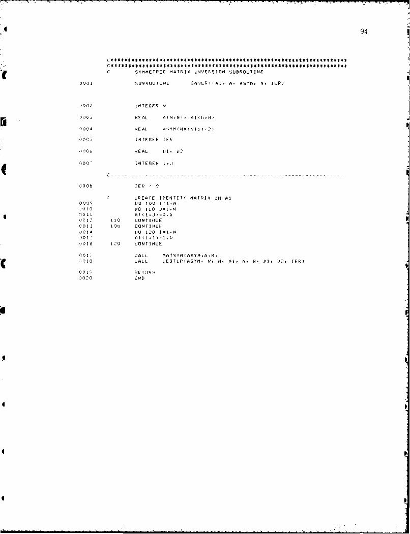
94

c SYMMETRIC MATRIX iNVERSION SUBROUTINE

0001 SUBROUTINE SN'JERT TA1 A. ASYM, N, IER'

00O2 INTEGER N

')003 REAL A(N,N, AI(N.N,

)004 KEAL AqYM(N*(N+I),2)

j005 INTEGER IER

206 KEAL II ,LI2

000- INTEGER t,.i

0006 1 ER 1; -

C 0REATE IDENTITY MATRIX IN Al

0001, 'L0 100 II,N

'010 t1O 110 J=iNO0L At(L.J)=Q.0

0012 110 CONTINUE

0013 lOU CONTINUE

u014 vO 120 I:IN

)015 AI(1, )=I.O

16 120 CONTINUE

O017 CALL MATSYM(ASYM,A.N,

)(018 LALL LEOTlF(ASYM, N, N, Al. N, 8, il, 112, IER)

C01 RETURNu02O END

95

iHI , i 1f41, iC. "1 N-AI-0 HAMERA CALIFRATIrN FROGRAM

o *$t *t mt * t **** $ $ ts * ** ** *****t** ************$ *$$ ****** ****** $

.001 IfA * 'IF TN' 4

1AN[,AF F 11 IN frF, i ,

j0 02 FI~ A 'T 1. 4 J4 1 4 k0EP 0F4i I T I F GNIA:tING f'i'E f l R'IP&L E C0nF INATES

u00 3 1,EFAL FiALrf 4

fOSITION *F LAS[P IN I AMERA COOR[IINATES (FIXED)

0004 REAL F IF TO( 4.12,CAL IEPRATION FATTEFN

0005 IFITEGEK NPUbNUMEBER OF EUB4LES IOUNI WY SUP

O00o RFAL FFICO(4),FHETA(5/

0007 REAL r05(4,4), FICT05(4.4), F ICT5O(4.4). UPJT05(4.4)

0008 REAL AFI1,3),XF3,),112,2,

0009 REAL AT(3, 12),ATA(3,3),ATAI (3,3),ATAIAT(3,12),ATASYM(6)

C FOR LEAST-SOUARES

uOlO REAL AXHAT( 12,2),MSERRXMSERRY, ITST(3,3)

C FOR CALCULATING MEAN-SQAURE ERRORS AND MATRIX INVERSION

jal1 INTEGER STAT

C STATUS WORD RETURNED b'f CAMAC

1012 INTEGER IER

C ERROK COPE RETURNED BY LSTSOS

)013 INTEGER I,II,J,10,iI0

C LOOH' COUNTERS

o0 14 REAL NWAIT

0015 DATf PHOMEO/90.O, 0.0. 60.0, 1.0/

)016 FATA FI CF'TO/ 0.0, -12.0, 0.0, 1.0,

1 12.0v O.o, 0.0 I. 1.0,

1 0.0, 12.0, 0.0, 1.0,

1 -11.0, O.0, 0.0, 1.0,7.79, -4.5, 0.0, 1.0,

.- ' - . .. .. .... .n "" ' , m m mii '' ''' a ' ' m mm ' m~~d,,i ~i,,.--, ,=- -'-aI-

96

L <.79. 4.5, 0.0, 1.0,1 -7.79, 4.5, 0.0, 1 0'

1 -7.79, -4,5, 0.0, 1.0.1 3.0, -5.20t 0.0, 1.0f

3.0, 5.20, 0.0, 1.0'1 -3.0, 5.20, 0.o, 1.0p1 -3.0, -5.20, 0.00 1.0/

L - - - -- - - - - - - - - - - - - - -- - - - - - - - - - - - - - - - - - - - - - - - - - - - - - - - - - - - - - - - - - -

J 0 1 7 WRITE(5,4)

0016 4 HORMATI/' CALIRATION ROUTINE ''

'019 WRITE(5,5)

oO2O FORMAT(/' ENTER X-Y COORDINATES OF OBJECT (IN CM):'/

1 X= '$,!302 REfAt(5,t)FU'J0( 1)

,)022 wRITE(5, )

002- F RMAT(' Y S,

0024 READ(5. )FOPJ0(2)

0025 F ' JO(3' .O,

0026 F'OBJO(4) = 1.0

002 WNITF,?

08 FORMAT( ' NUMBER OF SECONDS TO WAIT = ')

0029 REA[(5,*)NWAIT

MOVE ro HOME POSITION

0030 CALL MOVE(FHOMEO,TO5,THETASTAT)

FIND LOCATION UF LASER

0031 WkITE(58i0032 a FORMAT(' FINDING LASER'/)

0033 LALL SPUP(FPUP4, NPUI, 3,

0034 IF( NPUP .NE. I ) GOTO 999

0035 ALI MATMOV(FLASRC, PSURC(t,l), 4, 11

c CGET FARTIAL DATA IF ANY

003o 0 " 0

0037 WRITE(5,9)

)038 9 FORMAT(' ANY FARTIAL PATA IN CALPAT.DAT FILE (I=YES,-I=NO)? $)

019 READt(5,*)II

0040 IF(If .NE. 1) GOTO 20

0041 WkITE(5,29

0042 29 FORMAT(' PREVIOUS [AlA /)"

0043 CALL ASSIGN(J,'SY:CALAT.IPAT'.13)C KEAD IN ['ATA UNTIL EOF

0046 fJ I)047 GOTO 30

0048 35 CLOSE( UNIT 3 ,

,1I

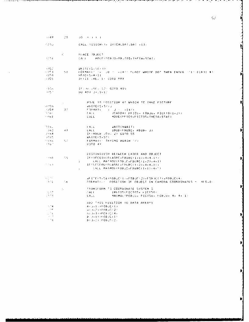
97

0 4 9 j0 >0

'2CALL )lSS I GN , S1 YC AL [I A r PA p1 3

CF L ACE 0L1E)-1FL('T

I> CAILI Mfly) P0OBJ0.0F(JT05,THETA.STAT)

)3 5K FOR MA T) Jo - [14' [LACE WHITE [lOT THEN ENTER I C1 ~Ri 5S

115IF' II NE, I' 0T0 Q99

K) FI F. I2 GO TO 4 00[1O 400 -1O= _10

MOVE 1T) FOSI 1TION AT WHICH TO TAKE FICTURE

WR5 IRETE ( S3 7U)1

'05? 37 ['iMAI( J = .14/1)CALL t VC AU[,4 ( PF I Co. F OBJo I PICF TO0( 1)

ICALL MiOYE(FFTCO,F*ICTOS,THETA,STAT)

J~bSI ALL WAIT(NWAIT,

*23 4? CALL 3PU( F PUPC , NF'UF .3A"064 [FINEIUb EU. 2) 6010 55,

WRITE(5, 52)FOFMAT), TRYING AGAIN '3010 4?

[iISTINOUISH E<ETWEEN LASFR AND OBJECT

IF(Y'ECE0U)PI ASRC,FIUEC) 1.1 ),4,4.0) )I ALL MATMO)FDJC,FL)EIC)I *2)4. I)

IFtYKFCE0Ue'TLASRL FF4HUPC)l -' ) 1.4, 4 .0) )tAL L MA T MOO ( F O[BJC I F PUE'C ( 1.I 1) 4, 4.

WV' 5, 6 jF OBJCI' * R0P3C 2) .FOE'i)( ) B OFJC(4

FqF11MAT)- F OS ITIO OF OFBJECT IN CAMERA COORDINATES -4F 5 .0

T PANSFORM To0 COORDIINATE SY(STEMCALL INYIOS(F ICTOS, kICT50

*CALL MATMUL)FOBJS. [[Cr50. [OB4JO. 4, 4.1

A1 I, fl[5HI FOSI 1T ION TO ['ATA ARRAYS

A' F, (IFElJC)

iJ F 0 PA C) 4

Pi F'J 2'F'O BJ52

E01 HE .YLCT U2 P: C It LOO f 2, IM

CNWETMI)TE WHERE THE T H IRD -O~E C T~lul H 1Pti

)"23 t-l Y13=FE'URI(2. I)+YELYD*C2*ITT24 E S y2 -3= F, pUEi'P 2 )VE LT2f IMF

tOY()=ES)TXl3+E5TX23),'

(02F ERRY=F[40E 23 --E AV 2

CLEYEL OFFESLTIMATI10N INFO F-OR FOURTH OB4JECT

2 1 ? IAL, -EFRRX 3 *TIM E 2T IMEM)**2+(EFRY3*(TIME2/TIME))**2'030 IEC3=3SOFT ,FLOA T ( IMAG ))

00iIF (ERRY3S. E L4.0)OGOTO I10)'f0 32 A N G2 =AAN ( FLOA I( ERR3/ERRX3 )

,234 :00 HNO2=3.14?:

RINE' THE QELOCIlY OF O)BJECT IN IMAGE THREE

'3% 1~ Y'QELTX=[E L X 3/TIMF'35 QELY3=DEFL (3v TIME

NflW ESTIMATE WHERE THE OBJECT WILL Pt

tS)(14F'PUP4 I. I +('.ELX2+ELX3 )*TIE4 'QEL[X2+YELX3 /2*TIMEI93Q E S T X'.14FI4 J 1+ YE L x3t*1IM E+ EL X 2+t) F LY3 /2 *T I ME

LSTX34=FPUT( 1 3)+ 'ELX2+YTLX3)/?"*TIME?S04 FT fl4 =FE4U( 21 )+ (VE YELE'-EYI*rTI ME4+-I E L Y 2+VEL Y3I/2*TT1ME

,')41 t5ST(24RE'U'( 2.u *'.ELY3*TIME+(YEFL(2+VEL (3)/2*TIMF2'(4Q, F S IY 34 F* B(41', 3)+ (YE L Y2 I'VJPL Y 3!2TIME P<43 t AYV( 3 ) ,'T1I4+EST%24+E51434) '3+'2003*OOS(AN-'"

'C,44 0091)4 )r(ESTYI4+ESTY24*ESTY34) /3fY.EE3*SINJ(ANO~i

4 ,-'nTO z,00

4 0 110 -30 1 I ').)47 CAM' 1 ' -F PUIP I'

'0 46F 6 3) 'V'IIfNIJ

'3)4 9 tA M) I , - rFAN 1 S.'20-F M (FOAM,' *. 4,S

'5 AL L F,&F'IFPCAm - 0 P ''rU ['15.- T

110

I LE E h'TP A T. T'IJ k F .cIFP 1 15F-,F TEME'ER 1784

THIS5 FZAL 'IDtI INS HE SUP;FUUT I NERT IAT I I N

C T H IS 1WRRk()T ITNF UILL( F ROVItIE AN E STfIMAT E rl THEL FOSI TIJN

JR THE 'EJEC T AT ;OMF SF EC IRFIEC ON T I N TINME') yI I v','' ,[ jr JEDr I> E'Cb E TIEEN I MAGFS I ANTL3

1X13.E-1T13 - STIMAIF OF 'JPJECI IN IMAGE 3 uSING

f ~~F OS ITION IN IMAGE 1 AS I N IT I Al rSI TI ON

I F35T X:13 , FS Tfe?3 1- rST IATE UKoPi UjC T I N IMAGE 3 USI 1N GFTOS IT IUN I N IMAGE ' AS I N I TI A I- F511T

INEGR FT(2. .EL Y2.rCTTO.FSqTC3.ESTYI3,ESTYP 3

T A 1) -I EFS TI MA TE FO0kR IJ F CT A T TGOS I TII N

ERR X3.ERRY3 - ERROR bETWEEN EST IMATE AND' (WSERVAT ION FORFOSITIION;

,NTEGER EAV(4).IERRXl.ERRY3

THLSE ARE THE ESTIMATE UF T'OSITT'1N 4 USING EiIFFERENIINIl IAL I-OSIT 1011

INTEGER ESTXl4,ESTX?'4.E5TX34.ESTYI 4,E5T724,ESTT34V It 53.VELY3 - VELOCITY VALUES IETWEEN IMAGES 21 ARE' 3

INTEGER VELX3, VE L Y -

HESE ARE IHE POSITION C-HANGES P4ETWEEN IHE FRAMES

*ITITELER PIELT). I'ELX3. [FLY2.TEELY3. ['ELTAX * LELTAA

LNTEIJER C

<7 rEAL rfS( 4 .4',FE V(4 r FU R (4F .C A M (4)1 ,'Pj 5 ( 4

PRE AL IHU P( 4,4' .-F(4 *TIME,TIMEC

iN I T IA LIE LONSTANTS;

lPE' THE POSI T ION 1,HANGES EETWEFN IMAGES 1 AND 2.r ANtI ALSO PETWEEN IMAGES 2ANt 3

-1 11EFL %2'Ul= EW P I 2* 2 -PPLIP I I

13 oELX3=F P1JP( I - 3 -1-PUP I .2)01 4 DELVY 3F EUE) 2. , -FRE 2.2' (

oEL T A X=PEJW- I 1 5 - F UIE, I *I

DELTAy=FPUE42,3-PUP .TI

LT 'HANGE EA AK ) HANCE

o038 253 [0 40 1:tCENT-COUtJTT,YCENT+COUNTY 90039 IZ.'RFIXE-(XCEN+XLTH/4, I'

0040 1F 1Z2.EOI.0OGOTO 40

0041 COUNT2<COUNT2+

0042 L.)ST2=I00Q4 3 40U CONTINUE

o044 IFlcOUNT2.LJ.3)GO1O 254

0 0453 YCENr2 =LASr2-(COUNr2/2,

u46b 254 (CE NITY C E NJI f rCENITI f Yf.EN TP)3

04 RETURN,)048 EN [1

108

c IHIS ROUTINE IS USED TO PROVIDE A MOREC. flICUhOTE EST I MAT LON OF TH4E OPJEC T S CENTEf<

'001 SUBEROUTINE ACENT(XCENI,YCENT,COUNTY,xLIN)

qoo: INTEGER XCEN1,YCENT,)(LTHCUNTv)003 INTEGER RFIxEL,XCENTL,XCENT2,(CENT1,YLENT20004 INTEGER COUNT1,COUNT2,,LAST1,LAST2

C ttITIALIZATION

0 0057 COUJNT 1=0,)006 CUUNT2=C

0007 XCENTI=yCENT0008 XCENT2= XCENT0009, YCENT1=rCENT00 10 (CEN T> ( fCEN T

0011l [itU 0 I=XCENT-XL-TN,XCENT+XLTH-)012 IZ1=RFIXEL(I,f(CENT-COUNTY/4)0013 IF(1Z1.EU).0)GOTU 100014 COUNTI1 C0UNT 1+ 100151 LAST~I=

0016 10 CONTINUE001- IP(COUNT1.LI.3,OOt) 2510018 %CENT1=LAST1- (COUNT1/2)

0019 251 D10 :o, ItXCENI-XLTH.XCENT+XLTI,)020 I"Z2RRIXEL (I. YCENT +COUNTY/4)0021., IF(I22.EIJ.0)GOTU 20'>022 COUNT2=COUNT2+I0023 LAST2=10024 210 CONTINUE0025, IF7COUNT2.LT.3)GOTO 25:'0026 XCENT2=LAST2- (COUNT2/2)

0027 252 XLCFN1 =1XCENT+XCENT1 FXCENT>-'/3

00 28 COUN TlI=00 0 29 CO0U N T20

)030 DO 3 0 1IZfC EN T -C0U N T Y ,YCE NT +CO0U N T Y0031 I / 1 RF' IXEL(XCEN r -XL FN/ 4.0032 IF(I21.EO.0fl3OTO 300033 COUNTI1 COUNT 1+10034 LASTI=I0 0 35 3 3 C 0N T tNIJ E00)3 6 IF(COUNT1.o1.3>0OTO 253

003?YCEN11tL6ST1-(COUNT1/2,

4 107

C05 :PB12)= PE4UP( 1:2) 256)

0057 RETURN0 0 Fj EN [

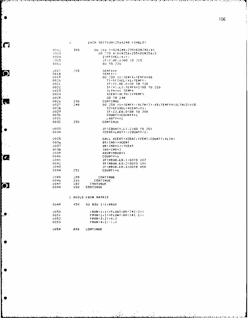
0 106

cEACH SECTION(256X2'40 PIXELS)

011- 300 [10 210 Y=t2*24O.239+D12*240.100)013 ['0 7120 X[Lul*256 ,255+[11*256,50014 2 'FlI XEL ( K,Y,,015 IF(Z.NE.0)GO 10 215001, GO TO 220

.,)01 215 TIEMFX= X0018 TEHFV'0019 VO 2'30 X1=rEMFXrEMFX+400020 21 'FFI EL (XI *TEMFY'0021 1F71I.NE.0h30 TO 2300 02 2 IF(X1.LT.TEMFX+2)OO 10 2200 0 23 ALTH=X1-TEMF*X0024 XCENT=XLTH/2+ TEMP*X

0025 00 10 2400026 230 CONTINUE002"7 240 ['0 250 (1=IEMP'Y-(XLTN/2)-15,TEMF'Y+(XLTH/2)+150028 22=RFIXEL(XCENI,Y1,0029 1F(Z2.EO.0)GO rO 2500030 COUNTY=COUNTY+100311 tASTY=T10032 250 CONTINUE

*0033 IF(COUNTY.LI.200O TO 2510034 YCENI=LASTY-(COUNTY/2)

00315 CALL ACENT(XCENT.TCENT,COUNTYeXLTH)003ct ER(IN1t)=XCEN10037 [R(INI+I)=YCENI0038 INE'=INft+20039 NPUP=N'UE+1a 0040 COUNTY=?10

0042' IF(NBUP.EO,2)0Ot0 100)0043 IF(NUB.EO.3)GOTO 4500044 251 COUNTY=0

0045 220 CONTINUE0046 210 CONTINUE0047 102 CONTINUE

*0048 100 CONTINUE

C BUILD' [Ed! MATRIX

0049 450 ['U 830 I=1,NPU4

0,050 r'E'UE (1,1)=FLOAT I R (2'*1-2))*0051 FPliB(2pI)=FLOAT([IR(2*I-1))

0052" F'U!'3 9I1=0. 00053 FBEUB4,I 1 .0

0054 830 CONTINUE

105

FILE F31.FIS t E'.'VI'ED 20 AUGUST 1984

THIS FILE CONTAINS THE SUBROUTINEf F 31-i. F TN

FILE F3B,FTf. r:EVISE 20 AUGUST 1984

THIS FILE C'ONTAINS THE SUBROUTINEf. F3B.FTN

.00 SUBROUTINE F3B(FBUBNBUB)

C THIS SUBROUTINE LOCATES THE POSITION OF THE OBJECTS

C WITHIN THE FRAME BUFFER AND REFERS ALL POSITIONS TO

C THE TOP LEFT QUA[DRANI . THI.

C ROUTINE WAS UPDATED 10 BE MORE ACCURATE WITH THE

C CENTER FINDING TECHNIQUE BY USINU THE SUBROUTINE

C ACENT' WHICH FIN).DS SEVERAL VALUES FOR CENTER LOOR-

C DINATES AI',i AVERAGES THEM TO DERIVE THE FINAL VALUE.

0002 INTEGER ,,,R'IXEL,2., I

C TEMF'X,TEMF'Y - INITIAL BOUNDARY COORDINATESXLTH - LENGTH OF INITIAL CHORD MEASURED ON OBJECT

0003 INTEGER TEMFXPTEMFYZ1,Z2,XI.TI.

C COUNTY - LENGTHH OF INITIAL CHORD IN Y DIRECTION

C LASTY - LOCATION OF LAST OBJECT PIXEL ON INITIAL CHORDXCENT,YCENT - ESTIMATES OF CENTER COORDINATES

0004 INTEGER XCENT,YCENI,COUNTYLAST'i

C DR - ARRAY CONTAINING CENTER COORDINATES

C IN'D - INDEX TO SFECIFIC VALUES IN DR ARRAY

C NBUB - NUMBER OF OBJECTS FOUND

0005 INTEGER DR(0: 10), INfiNBUB0006 INTEGER 1.tI',,1D2

C PBLIB - REAL ARRA( CONTAINING OBJECT VECTORS IN CAMERA COOR.

0007 REAL FB,.UB(4,4I- iNITIALIZE LONSTANTS

0005 i'HIJH=G 50009 1 N1= ,)

START FROCESSING (HE FRAME BUFFER

0010 [' lOo D I,.

0011 DO 102 DI=0,I

I

• . . . .S

1 04

)001 SU ROUT I N17 L:ELAYfN)

C SUBRrIUTIPIL DELAY WILL FROVI[L A DELAY OF N SECS.

,002 TNTEGER LM0003 REAL N.)004 .-i=40 WrN

0005 11U F L=I)006 LALL [iy

0007 t. COHTINUEJ008 ETURN

000S END

4I

S

S

S

S

.. , .. ..., ' +- ... _ . • " .. ..: _, . -" , ; -i i~ " .', . ..., ---". . "'9

103q

, THIS SUBROUTINE WILL 'RODUCE THREE PICTURES IN AC SINGLE FRAME IUFFE,.

)001 5UEROUTINE I SNAFS ( TIME, T IME2, FIUBN NUB)O002 INTEGEK NEUF,)003 NEAL tIME,TIME2,F'BU

C INITIIALIZE CONSTANTS

i: TAKE THREE PICTURES IIME* SECS. APART AND STORE

C IN FRAME EUFFER.

,,004 cALL PAN ()ooo CAlL SCROLL(0,0 6 C ALL ZOOM(I,1)

0007 CALL SNAF

.)009 LALL P'AN(256)

000 CALL VIEW

)010 LALL LELAY(TIME)001i CALL SNAF

,.,) I , i-ALL P'ANI t )

001 , CALL SCROI. ( 240))14 .*ALL VIEW0015 CALL DEl A TIMF0016 cALL NAF

)oI- CALL PAN0 ,

)01 CALL '$CROLLO

0019 50 CALL F3P(F'BUIBN NBU

o)020 -ETURN002I ENt

Ci

4B

4; - . " . - . " " - . .. , • -, . - - . . .

102

038 ALL T SNAFS( T I ME, T I ME2, F'4U1, NPUB003s CL L RE T C A T T I ME. T IMC2,FUB, F, REV, F'CU, TO5, FCAMF'O4J5, C'040 ,FkC.EO.O.)GOTO 160

0041 IU I1 J=1.4

3042 O(J)=I-REV(J)004; ' I CONTINUE

)014 OTO 190

004S 180 CALL FORF'(FF ,5F0,.T05.

4JF'DATE FREV VALUES

)04, F 'E'' ( I , - P')( I ,)04- REV =F 0 1

004 F 190 CAl L IYFI(F(,TOtTHETA,STATj

049 t-LL WAIT(TIME)

0050 200 CONTINUE

,,hll I TOF'

005: END

I

C

- I

101

.,ACKAGEI 30FTWARE(IMAGE TECHNOLOGYINC.)

000o CAI L SELGRF(1,J007 CALL JYNC(O)0006 CALL FBINIT0009 ALL APINIT0010 CALL LUINIT)011 , ALL. V IDCHN (O0

JNITIALIZE A BINARY LUT(.'THRES'=0,BLACK)

OO1 WRITC(,,999,3013 ?99 &ORMAT(IX,' PLEASE INPUT THRES FOR ZERO INTENSITY')0014 F:EA( , 998)THRESJot, ?98 F'ORMAT(13)001t CALL SELLUT(0,0;301' uIO 1 I-JTHRES

0016 CALL SETLUT(I,0j0019 CONTINUE0020 DO 2 1 -THRES+1,255J021 CALL SETLUT(I,2S5)002: 2 CONTINUE

SELECT OUTPUT CHANNEL AND VIEW

0023 CALL SELLUT(1,0)0024 CALL VIEW

f-C F0IIILt' INITIAL TO5 MATRIX

3025 CALL MOVE(F'HOME, fOSPHETASTAT)

C INPUl TIME BETWEEN INITIAL SNAPSHOTS

0026 WRITE(5,99)

,027 99 lORMAT(1X,'INPUT rIME(IN !ECS,) BETWEEN IMAGES.')0026 REA(bo,1)TIME)029 10 FORMAT(F10.4)

C INPUl TIME ESTIMATION POINT,)030 WRITE(5,98)0021 ?O fORMAT(1X,'INPUT CIME(IN SECS.) FOR FINAL POSITION.')0032 READ(b,10)TIME2

* iNITIALIZE ROBOT POSITION FUR CATCH UF MODE

0033 PREV(1)=90.0

J034 iREV(2)=0.00035 PRrV(3)=60.O0036 rREV(4)=1.0

START TO TRACK OBJECI

J037 1O 200 1=1,100

APPENDIX B: COMPUTER PROGRAM LISTING

HIS FROGRAM CONTROLS THE IMAGE PROCESSING ANDI RilpOl If: HOVEMENI FOR A SIMPLL TRACKING APPLi-C, :-ATION OF THE I", INDUSTRIAL ROBOT. THE SYSTEM

IMI'LCMENT, A TYP*E 01 VISUAL CONTROL BY EXTRACTING'OSITIONAL DATA fHROUGH THE USE OF AN IMAGE

COUISITIOH SYSTEM.A_3T REVISE! ON DECEMBER 05,1984

P~flI%< Jul. I. O'CDONNELL

:ECESSARY VARIABLES

Tnl FLAG TO SIHNAL PROPER COMPLETION OF MOVEBL B JALUE OF NUMBER UF OBJECTS FOUND-

rHREb - THRESHOLli VALUE FOR BINARY IMAGE- FLAG DENOTING CATCH UP ROUTINE IN EFFECT

4 C£ol IHTEUEI< STAT,NBUB, tHRESC

iIME - TIME F'ERIOD BETWEEN SUCCESSIVE IMAGES

lIHE., - ESTIMATION TIME PERIOD-HOME - ARRAY LONTAINING IHE 'HOME' VECTOR FOR P5

10 (4,4) - GENERAL TRANFORMATION MATRIX FROM LINK 5COORDINATES TO BASE (0) LOORDINATES

f TCtj( ,4 - GENERAl TRANSFORMATION MATRIX FROM CAMERACOORDINATES TO LINK 5 COORtINATES

0002 REAL TIMETIHEJ,PHOME(4),TOS(4,4),TCS(4,4J7HETA(5) - mRRAY CONTAINING THE FIVE ANGLES WHICH DISCRIBE

C THE ORIENTATION AND POSITION OF THE P7FREV - ARRAY OF VALUES CHAT HOLD THE PREVIOUS POSITION OF

THE ROB0T IN BASE COORDINATES. THESE VALUESARE USE' WHEN THE OBJECT IS MOVING VERY SLOW

C I'Cuh - ARRAY USED BY SUBROUTINE To STORE CURRENT POSITIONOF OBJECT IN BASE COORDINATES

C [CAN - ARRAY USED BY SUBROUTINE TO HOLD LAST IMAGE COORDINATES'OBJ5 - ARRAY FCAM TRANSFORMED INTO LINK 5 COORDINATESP,, - THIS ARRAY CONTAINS THE ESTIMATED POSITION OF THE

OBJECT AT THE ESTIMATION TIME IN BASE COOP-

DlI NA TES

4 J003 *;EAL THETA(5),F'CUR(4),h'OBJ5(4),P'CAM(4),F REV(4),FO(4)PEUB(',4) - ARRAY CONTAINING THE CAMERA COORDINATES OF

iHE MOVING OBJECTu- (4- ARRAY CONTAINING3 THE ESTIMATED POSITION OF THE

MOVING OBJECT IN LINK 5 COORDINATESP'(4) ARRAY CONIAININ THE ESTIMATED POSITION OF THE

MOVING OBJECT IN CAMERA COORDINATES

0004 REAL P'BU (4,4),P(4),P14

.NITIALIZE CONSTANTS

000C 'A( FHOME/90,U.OO.60.O,1.0,

SNITIALIZE IMAGING EOUIPMENT USING

100

!'U

1 99

0108 WRITE(5.Th0'0109 760 tOR'MAT( /IAlA *ATAI'/)

0110 CALL. FRIMAT(1TST, 3, 3.9

0111 P99 CLOSE( UJNIT 5

0113 ENEI

C F-RINT OUT UFESATECI ['ATA0079 10D 90 JJ'I.120080 WRITE(5,9U)A(JJe 1).A(JJ.2fl;A(JJ,3) .8(JJ.1 ) g(JJ,2)C.0081 91 FORMAT( ',3 F10.,t,7X,2F10.50082 90o LONTINUE

C SAVE IN PARTIAL RESULTS FILE0083 hRITE(3999)A(J.1 ).A(J,2) *A(J.3fl14(J.I),IUJ,2)0084 99 FORMAT(' ',5F15.8i

0085 400 LONlINUE

0 0 8o WRITE(5.17i0087 17 FORMAT(//)

ooBCALL NOVEU-F'HOMEO.T05.THETA.STAT)

1. SOLVE FUN COEFi ICIEmrs0084 CALL LSTSOS(A,X.,4pT,ATA,OTAl.4A1AT,ArASYM.12,3,2. IERI

OUTPUT COEFFICIENTS TO TTY ANTI CAMCON.E'AT FILE

0090 WRITE(C5, 200 x (1 ,)*XC 2.1).*XC 3'1) ,X (19*2),X( 2,2) 'XC3,2)

*0091 200 FORMAT(' f5C(1I,1I) ' F15.8/1T5CC1,2) = ',F15.8/

T5C( 1 4) = ' FIS.B/1T5C(2,l) = 'PFIS.8/

T5CC2t.) = ',F15.8/IT5CC2,4 = ',F15.8/)

J092 CALL ASSIGNC2.'SY:CAMCON.IIAT'913)C ~~~0093 W I TE (2,210) X 1l,.XC 2 1) ,X (3.1). X(1 .2) .XC2,2). XC3.2)0094 210 FORMAT(6CF15.8/))0095 CLOSE( UNIT=2I

C CALCULATE MEAN-SQUARE ERROR

009o CALL MATMUL-(AXHAT.A,X. 12.3.2)009? MSERRX=0.00098 MSERRY=0.O

90099 £10 500 11=191210100 MSERRX=MSERRX+(E'CII'1 -AXHATCII.1))**20101 MSERRY=MSERRT + ((11,2) -AXHAT (11.2)) fl20102 500 CONTINUE0103 MSERRX=MSERRX/12.O0104 MSERRY=MSERRY/12 .00)105 WRITE (5.550' MSERRX ,MSERRY01%o 55u FORMAT(' MEAN-SOUARP ERROR IN X = ',F15.5/

*I MEAN-SQUARE ERROR IN Y = ,PF15.5)

C CHE':K OUl INVERSION OF ArA MATRIX0107 CALL MATMUL(ITST. MTA. ATAI. 3p 3. 3)

112

COMPARE 'REVIOUS POSITION WITH CURRENT POSITION

( 0052 IF((A8S(PCUR(I i -F REV(1)). L I. 2. 0 .AND,.(APS(F'CUR (2)-F'FREV(2)) .L T '.0) )GOTO 5a83

0053 PRE'J( 1 )=F'CLIPR Ij0054 rREV(2)=F'CUR(2)

0055 583 F(1F=FREV(I,0056 F( 2 )=FRE ( 2

0051 P(3) =60.O0058 4)= .0

0059 WRITE(5,26,0060 26 -ORMAT(IX, CATCH UP MODE')0061 COTO 610

C FORM THE F' VECTOR

0062 600 P(1)=(FLIIAT(EAUJ(3))*2) 25o,063 F(2)=(FLOAT(EAY(4) )*2)-2400064 F(3)=o.u0065 '(4)=1.0

006o 610 RETURN0067 ENE,

I

.C%.° .% °_-

S 113

IHS OUT NE oRms HE NECESSARY -F- VECTOR 10 MOVE R01E<0T

.SSIGN Alt) 2 ru cAmrt4.I.4i

'003 LALL ASSIN', 2SY:CAMCOt4.[fAJ .13)

S , rGrI CAM-T, '01 CONSTAN ,

000-1 CLOSE'UNfl=2i

''006 r ',( I ) * F I + P F2 4 40)00f)7 F ' (2 C * 1 +)VP ( 2) Y

)010 LALL rIATMUL'*P0, ro7,F5,4,4,1

0011 RETURN,'012 LNEP

I

S

0

la FILMED

• 4-85

* DTIC

ROBOTIC MANIPULATOR THROUGH THE USE OF -iM … · -im 933 positioning of a robotic manipulator...

Documents

Transcript of ROBOTIC MANIPULATOR THROUGH THE USE OF -iM … · -im 933 positioning of a robotic manipulator...