
Robot introspection through learned hidden Markov modelskuipers/readings/Fox-aij-06.pdf · 62 M....
55
Artificial Intelligence 170 (2006) 59–113 www.elsevier.com/locate/artint Robot introspection through learned hidden Markov models Maria Fox a,∗ , Malik Ghallab b , Guillaume Infantes b , Derek Long a a Department of Computer and Information Sciences, University of Strathclyde, 26 Richmond Street, Glasgow, G1 1XH, UK b LAAS-CNRS, 7 Avenue du Colonel Roche, 31500 Toulouse, France Received 1 December 2004; accepted 6 May 2005 Available online 1 September 2005 Abstract In this paper we describe a machine learning approach for acquiring a model of a robot behaviour from raw sensor data. We are interested in automating the acquisition of behavioural models to provide a robot with an introspective capability. We assume that the behaviour of a robot in achieving a task can be modelled as a finite stochastic state transition system. Beginning with data recorded by a robot in the execution of a task, we use unsupervised learning techniques to estimate a hidden Markov model (HMM) that can be used both for predicting and explaining the behaviour of the robot in subsequent executions of the task. We demonstrate that it is feasible to automate the entire process of learning a high quality HMM from the data recorded by the robot during execution of its task. The learned HMM can be used both for monitoring and controlling the behaviour of the robot. The ultimate purpose of our work is to learn models for the full set of tasks associated with a given problem domain, and to integrate these models with a generative task planner. We want to show that these models can be used successfully in controlling the execution of a plan. However, this paper does not develop the planning and control aspects of our work, focussing instead on the learning methodology and the evaluation of a learned model. The essential property of the models we seek to construct is that the most probable trajectory through a model, given the observations made by the robot, accurately diagnoses, or explains, the behaviour that the robot actually performed when making these observations. In the work reported here we consider a navigation task. We explain * Corresponding author. E-mail address: [email protected] (M. Fox). 0004-3702/$ – see front matter 2005 Elsevier B.V. All rights reserved. doi:10.1016/j.artint.2005.05.007
Transcript of Robot introspection through learned hidden Markov modelskuipers/readings/Fox-aij-06.pdf · 62 M....
Artificial Intelligence 170 (2006) 59–113
www.elsevier.com/locate/artint
Robot introspection through learned hiddenMarkov models
Maria Fox a,∗, Malik Ghallab b, Guillaume Infantes b, Derek Long a
a Department of Computer and Information Sciences, University of Strathclyde, 26 Richmond Street,Glasgow, G1 1XH, UK
b LAAS-CNRS, 7 Avenue du Colonel Roche, 31500 Toulouse, France
Received 1 December 2004; accepted 6 May 2005
Available online 1 September 2005
Abstract
In this paper we describe a machine learning approach for acquiring a model of a robot behaviourfrom raw sensor data. We are interested in automating the acquisition of behavioural models toprovide a robot with an introspective capability. We assume that the behaviour of a robot in achievinga task can be modelled as a finite stochastic state transition system.
Beginning with data recorded by a robot in the execution of a task, we use unsupervised learningtechniques to estimate a hidden Markov model (HMM) that can be used both for predicting andexplaining the behaviour of the robot in subsequent executions of the task. We demonstrate that it isfeasible to automate the entire process of learning a high quality HMM from the data recorded bythe robot during execution of its task.
The learned HMM can be used both for monitoring and controlling the behaviour of the robot.The ultimate purpose of our work is to learn models for the full set of tasks associated with a givenproblem domain, and to integrate these models with a generative task planner. We want to show thatthese models can be used successfully in controlling the execution of a plan. However, this paperdoes not develop the planning and control aspects of our work, focussing instead on the learningmethodology and the evaluation of a learned model. The essential property of the models we seekto construct is that the most probable trajectory through a model, given the observations made bythe robot, accurately diagnoses, or explains, the behaviour that the robot actually performed whenmaking these observations. In the work reported here we consider a navigation task. We explain
* Corresponding author.E-mail address: [email protected] (M. Fox).
0004-3702/$ – see front matter 2005 Elsevier B.V. All rights reserved.doi:10.1016/j.artint.2005.05.007
60 M. Fox et al. / Artificial Intelligence 170 (2006) 59–113
the learning process, the experimental setup and the structure of the resulting learned behaviouralmodels. We then evaluate the extent to which explanations proposed by the learned models accordwith a human observer’s interpretation of the behaviour exhibited by the robot in its execution of thetask. 2005 Elsevier B.V. All rights reserved.
Keywords: Stochastic learning; Hidden Markov models; Robot behaviour
1. Introduction
The goal of the work described in this paper is to automate the process of learning howa given robot executes a task in a particular class of dynamic environments. We want tolearn an abstract model of the behaviour of the robot when executing its task solely on thebasis of the sensed data that the robot records when performing the task. Having learnedan execution model of this task we want to use the model to reliably predict and explainthe behaviour of the robot carrying out that same task in any other environment belongingto the class. This paper describes how we have approached this goal in the context of anindoor navigation task, and how successful we have been in learning a reliable behaviouralmodel.
1.1. Motivation
The work presented here illustrates that it can be advantageous to approach a complexartifact, such as an autonomous robot, not from the usual viewpoint in robotics of thedesigner, but from the observer’s point of view. Instead of the typical engineering questionof “how do I design my robot to behave according to some specifications”, here we addressthe different issue of “how do I model the observed behaviour of my robot”, ignoring, inthis process, the intricacy of its design.
It may sound strange for a roboticist to engage in observing and modelling what a ro-bot is doing, since this should be inferrable from the roboticist’s own design. However,a modular design of a complex artifact develops only local models which are combinedon the basis of some composition principle of these models; it seldom provides globalbehaviour models. The design usually relies on some reasonable assumptions about theenvironment and does not model explicitly a changing, open-ended environment with hu-man interaction. Hence, a precise observation model of a robot behaviour in a varying andopen environment can be essential for understanding how the robot operates within thatenvironment.
We are proposing in this paper a machine learning approach for acquiring a particu-lar class of behaviour models of a robot. The main motivation for this work is to buildmodels of robot task execution that are intermediate between the high level representationsused in deliberative reasoning, such as planning, and the low level representations usedin sensory-motor functions. A high-level action model, such as a collection of planningoperators with abstract preconditions and effects, is certainly needed in high level missionplanning. However, it is of limited use in monitoring and controlling the execution of plans.

M. Fox et al. / Artificial Intelligence 170 (2006) 59–113 61
These functions need a more detailed model of how an action breaks down, depending onthe environment and the context, into low-level concurrent and sequential sensory-motorprimitives, and how these primitives are controlled. On the other hand, the representationsused for designing and modelling sensory-motor functions are necessarily too detailed.They are far too complex to be dealt with at a planning level, or even for execution moni-toring. The latter requires intermediate level models, either hand-programmed, learned, orrefined through specification and learning.
Other authors have considered how intermediate level descriptions of task executionmight be used for designing a robot, i.e., how the corresponding models might be encodedand exploited within a plan execution framework. We are not concerned with programmingthe low level control of the robot but with providing the means by which a robot can intro-spect about the development of its behaviour in the execution of a task. We rely on hiddenMarkov models (HMMs) [25] as the intermediate level representation of this behaviour.Since these models are built empirically, they take into account the dynamics and uncer-tainty of the real execution environment. The resulting behavioural models provide a wayin which the controller can reason about the robot behaviour in the context of executing atask.
Our focus here is not on learning topological or metric maps for robot navigation. Oth-ers have considered this problem in depth [1–4] and shown that navigation with respectto a given environment can be dynamically improved as the robot interacts with its envi-ronment. The use of stochastic learning techniques to improve robot navigation in a givenenvironment is therefore quite well-understood. We are concerned with learning abstractmodels of how a robot performs a compound task, whatever that task might be. Navigationis an example of such a compound task.
1.2. Approach
Our objective is to be able to predict and explain the robot’s behaviour as it undertakes acompound task in the uncertain real world. In reality the robot passes through a number ofabstract behavioural states, some of which can be distinguished and identified by a humanobserver. For example, when picking up an object in its grippers a robot might be in thestate of positioning with respect to the object, approaching it, grasping it, knocking into it,lifting it, and so on.
To illustrate the kind of model we are interested in learning, Fig. 1 shows a high levelstate transition model of a pickup task (this is an artificially simplified example that wasnot learned from real data). Time is abstracted out of the model and it is assumed that amonitoring process tracks how often the robot revisits the same state.
It can be seen that, according to the model, the probability of knocking into the objectis 0.2 when the robot is positioning itself and when it is in the approaching state, havingpositioned itself ready to grasp the object. The probability of looping on the positioningstate is high, suggesting that the robot often fumbles to get into a good grasping position.The trajectories through this model that are actually followed by the robot might revisit thepositioning state multiply often and it might be that the state of knocking into the objectis entered most frequently when this is the case. Using the HMM to identify the mostprobable trajectory leading out of the current state provides a monitoring system with a

62 M. Fox et al. / Artificial Intelligence 170 (2006) 59–113
Fig. 1. The compound task of picking up an object.
powerful ability to determine the most likely outcome of the robot’s current behaviour. InSection 7 we discuss how the structure of the HMM can be exploited by such a monitoringsystem.
The behavioural states of the model are hidden, because they cannot be sensed directlyby the robot. The robot is equipped with noisy sensors from which it can obtain only anestimate of its state. A hidden Markov model (HMM) represents the association betweenthese noisy sensor readings and the possible behavioural states of the system, as well as theprobabilities of transitioning between pairs of states. The HMM is therefore ideally suitedto our objectives. Our approach is to learn a HMM that relates the sensor readings made bythe robot to the hidden real states it traverses when executing its task, in order to equip therobot with the capacity to monitor its progress during subsequent executions of the sametask.
Our work makes several innovations. First, we address the problem of learning the struc-ture as well as the parameters of the HMM, using a structural learning approach based onKohonen network clustering. We begin with no prior knowledge about how many statesthe HMM will have, or what the relationship between states and observations might be.Second, we learn an HMM that is independent of the physical locations at which activitytakes place. The states we are concerned with are abstractions of the behavioural statesof the robot. Expectation Maximization (EM) [5] is used to estimate the transition prob-abilities between them based on multiple sequences of robot observations, each sequencecorresponding to the observations made by the robot during an execution of the compoundtask.
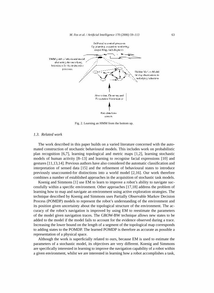
Fig. 2 gives an overview of the whole learning process, and suggests how the resultingmodel might feed into high level deliberative reasoning processes. In this paper we focuson the processing and clustering of raw sensor data leading to the construction of HMMs.As we discuss in Section 7, these models represent behavioural abstractions that can beused by high level deliberative processes.
We show that it is possible to learn high quality HMMs using a fully automated ap-proach. Although some questions remain to be answered we believe that our work consti-tutes an interesting step towards the acquisition of a predictive and explanatory model ofrobot behaviour that is grounded in its actual sensed experience in reality.
M. Fox et al. / Artificial Intelligence 170 (2006) 59–113 63
Fig. 2. Learning an HMM from the bottom up.
1.3. Related work
The work described in this paper builds on a varied literature concerned with the auto-mated construction of stochastic behavioural models. This includes work on probabilisticplan recognition [6,7], learning topological and metric maps [1,2], learning stochasticmodels of human activity [8–13] and learning to recognise facial expressions [10] andgestures [11,13,14]. Previous authors have also considered the automatic classification andinterpretation of sensed data [15] and the refinement of behavioural states to introducepreviously unaccounted-for distinctions into a world model [2,16]. Our work thereforecombines a number of established approaches in the acquisition of stochastic task models.
Koenig and Simmons [1] use EM to learn to improve a robot’s ability to navigate suc-cessfully within a specific environment. Other approaches [17,18] address the problem oflearning how to map and navigate an environment using active exploration strategies. Thetechnique described by Koenig and Simmons uses Partially Observable Markov DecisionProcess (POMDP) models to represent the robot’s understanding of the environment andits position given uncertainty about the topological structure of the environment. The ac-curacy of the robot’s navigation is improved by using EM to reestimate the parametersof the model given navigation traces. The GROW-BW technique allows new states to beadded to the model if the model fails to account for the evidence observed during a trace.Increasing the lower bound on the length of a segment of the topological map correspondsto adding states to the POMDP. The learned POMDP is therefore as accurate as possible arepresentation of a physical space.
Although the work is superficially related to ours, because EM is used to estimate theparameters of a stochastic model, its objectives are very different. Koenig and Simmonsare specifically interested in learning to improve the navigation capability of a robot withina given environment, whilst we are interested in learning how a robot accomplishes a task,

64 M. Fox et al. / Artificial Intelligence 170 (2006) 59–113
whatever the task may be. In the work we describe in this paper we use the navigation tasksimply as an example of a compound task. The states of our learned model correspond toabstract behavioural states, such as obstacle avoidance, not to physically grounded statessuch as one metre from a corridor junction. This is a significant difference because ourmethod is task-independent. The states are acquired automatically by means of the cluster-ing of sensor input and their veracity is established by evaluating the predictive power ofthe resulting HMM.
Several authors have considered how intermediate level models might be used fordescribing the execution of a task. For example, RAPS [19] and Structured Reactive Con-trollers [20] provide the low level programs into which actions at the task-planning leveldecompose at the executive level of the robot architecture. RMPL [21] and TDL [22] areexamples of languages that have been developed for the specification of such programs.These programs might be hand-coded or they might be acquired by learning or by inter-pretation of learned models. The Procedural Reasoning System (PRS) [23] is a furtherexample of an architecture that supports the relationship between high level plans and ex-ecution.
The work done in gesture [11,13,14] and facial expressions [10] recognition is closelyrelated to our concern. If an HMM is used to model the probabilities of a human facetransitioning between different expressions, and these expressions are linked to emotionalstates and actions, it becomes possible to predict the most likely next action of a personbased on interpretation of his facial expression. Similarly, if gestures are associated withactivities a learned HMM can enable the immediate goals of a person to be predicted on thebasis of his recent and current gestures. This work is similar to our own because the statesof the learned HMMs are behavioural states of the subject and are not associated with thephysical location of the subject.
Liao, Fox and Kautz [8] use learned models to predict human transportation behaviours.They can detect when a person’s behaviour deviates from their normal pattern by evaluat-ing the likelihood of an observed behaviour in the context of a learned model. Osentoski,Manfredi and Mahadevan [9] learn models of human behaviours in order to provide robotsfunctioning in human environments with the capacity to predict and explain human activ-ities. In both studies the HMM is used to predict the probability that certain activities arebeing undertaken at certain physical locations. The structure of the HMM is hierarchical,with the lowest level corresponding to a physical network of locations and higher levelscorresponding to the activities that typically take place at these locations. Thus, the work isconcerned with relating activities to physical space and its emphasis is therefore differentfrom our own.
In our work the association between the sensor readings of the robot and its behaviouralstates is learned by means of Kohonen network clustering. A closely related approachin the literature is the work of Oates, Schmill and Cohen [15] in which dynamic timewarping is used to cluster multivariate time series sensor data, or experiences. Oates etal. present an unsupervised method of clustering experiences into classifications of actionoutcomes enabling a robot to interpret its state in a way that accords well with humanjudgements. The objective of their work is to identify cluster prototypes that form the basisof an ontology of activity that can lead to the automated construction of operator models.
M. Fox et al. / Artificial Intelligence 170 (2006) 59–113 65
The way in which we use the results of the clustering phase is different and a more detailedcomparison follows later in the paper.
1.4. Layout of the paper
In Section 2 we formulate the problem we are addressing, specifying the notation wewill use in this paper, introducing the main methods and algorithms and defining the keyterms that we will use. In Section 3 we discuss data clustering using the Kohonen networkclustering approach. We describe how an initial collection of behavioural states is refinedby the clustering process. We then explain the process of building an initial sensor modelusing the code book approach, and show how all of the remaining parameters of the HMMare initialised. We then review EM, describing how the initial parameters are iterativelyreestimated. Section 4 describes the robot and its array of sensors, the data we collectedand the class of environments we studied. We explain how the observable outputs of therobot are processed to extract the features used for clustering, and how the feature vectorswe used are constructed. In Section 5 we discuss the implementation of the entire learningprocess, showing how the EM process was integrated with the clustering phase in oursystem. The EM process requires evidence to be provided, and we explain how sequencesof observations are generated for this purpose.
In Section 6 we describe the evaluation strategy we have devised for determining thequality of the learned HMM in terms of its power to explain the robot’s behaviour fromits observations. Using the Viterbi algorithm [24] we construct the sequences of states thatbest explain the observation sequences, and then we compare the Viterbi sequences withwhat the robot did in reality. This comparison relies on a human observer’s interpretationof the robot’s real behaviour. We discuss the strengths and weaknesses of this approach.
Finally, in Section 7, we turn to a discussion of how the learned models can be used inthe monitoring and control of robot behaviour. Although this is not the focus of the currentpaper we explain how the HMMs can enable a robot to predict entry into an undesired stateand to take averting action in time to avoid a failure. We discuss how HMMs can be usedin combination with policies and plans to support a robot in achieving high level missiongoals.
2. Formal problem statement
There are three main problem components to define: the model of a task as a finitestate transition system, the clustering of the observation space into a finite evidence space,and the definition of the finite behaviour state space. For each component we will presentthe assumptions that we make concerning the component and its role in the problem, theformal definition of the component and a brief introduction to the algorithm that is usedto construct instances of the component. In the following section we present details of thecore algorithms introduced here.
In our definitions we use n and m as index variables indicating the lengths of sequencesin the context of each definition. These variables should be interpreted as locally definedwithin the scope of each definition.

66 M. Fox et al. / Artificial Intelligence 170 (2006) 59–113
2.1. Models and tasks
Assumption. The robot behaviour for task T can be conveniently modelled by a finitestochastic model.
Definition 1. A stochastic state transition model is a 5-tuple, λ = (Ψ, ξ,π, δ, θ), with:
• Ψ = {s1, s2, . . . , sn}, a finite set of states;• ξ = {e1, e2, . . . , em}, a finite set of evidence items;• π :Ψ → [0,1], the prior probability distributions over Ψ ;• δ :Ψ 2 → [0,1], the transition model of λ such that δi,j = Prob[qt+1 = sj | qt = si] is
the probability of transitioning from state si to state sj at time t (qt is the actual stateat time t);
• θ :Ψ ×ξ → [0,1], the sensor model of λ such that θi,k = Prob[ek | si] is the probabilityof seeing evidence ek in state si .
Under the Markov assumption the state of the robot at time t depends only on its stateat time t − 1, so that λ produces a hidden Markov model.
Definition 2. A history h = 〈e1 . . . en〉 is a finite sequence of evidence items.
The algorithm we are using to build the model is the well-known technique of Expecta-tion Maximization (EM) [25], also called the Baum–Welch algorithm [26]. Given a set ofhistories and the initial parameters of a HMM—an initial sensor model, an initial transitionmodel and a prior state distribution over the states in Ψ —EM iteratively reestimates theHMM parameters. On each iteration EM estimates the probability, or likelihood, of the ev-idence being seen given the HMM estimated so far. It then updates the model parameters tobest account for the evidence. When the estimated likelihoods are no longer increasing EMconverges. The probability at convergence is represented as the maximal log likelihood: thebest local estimate possible given the evidence and the learned model. Log likelihood isused because the probability of a particular observation sequence being seen in a complexmodel is typically low enough to challenge the arithmetic precision of the machine. It iswell known that EM has a tendency to converge on local maxima, but careful selection ofthe initial HMM parameters can help to mitigate this tendency.
The inputs to the EM algorithm are: a finite set of histories, H = {h1, . . . , hn}, corre-sponding to the training data associated with n executions of task T , and an initial model,λ0 = (Ψ, ξ,π, δ0, θ0). The output is a learned stochastic model λ corresponding to a hiddenMarkov model describing the task T .
2.2. Clustering the observation space into evidence
Assumption. A multi-dimensional non-finite observation space can meaningfully bemapped into a finite set of evidence items.

M. Fox et al. / Artificial Intelligence 170 (2006) 59–113 67
We refer to the collection of sensor readings that can be made by the robot, at some pointin time, as an observation. Each reading gives the value of a certain primitive feature whichwe call a raw feature, such as the heading of the robot, the speed at which it is travelling,and so on. The observation space is therefore defined by the particular collection of sensorswith which the robot is equipped and its interaction, by means of these sensors, with theenvironment.
Definition 3. A k-dimensional observation space is defined as Φ = γ1 × γ2 × · · · × γk ,where:
• γi ⊆ �;• A raw feature is defined to be a function fi : robot × env × time → γi mapping the
sensory-motor and environmental context of the robot, at a time t , to a value in therange γi , thus partially characterising the behaviour of the robot at some instant t intime.
Definition 4. An observation is a point in observation space.
Although we describe fi as a function of the robot and its environment, we have noaccess to this function or control over how it produces its mapping to raw feature values.Raw feature values are determined by the low level robot control software upon whichthe learning pursued in this project is based and the interaction between the robot and itsenvironment. We can sample fi for specific values of its arguments.
Under our assumption mappings exist from the observation space Φ to a set of abstractobservations ξ . We call the elements of ξ evidence items. We first define a trajectory,then explain how the construction of trajectories allows the set ξ and a mapping to beconstructed by means of the clustering of the observation space.
Definition 5. A trajectory τ = 〈o1, o2, . . . , on〉 is a finite sequence of observations charac-terising a single execution of the task T .
Our intention is to discretise the non-finite observations, Φ , of the robot into a finitecollection of distinct evidence items, ξ , and to determine a mapping cluster :Φ → ξ . Thisrequires a process of abstraction and the combination of raw feature values across obser-vations. A single observation is not informative enough to enable us to determine how therobot’s behaviour develops over time. If we consider a single observation taken at time t
the raw feature values will reveal very little about how the robot’s behaviour has evolvedup to that time, or will evolve after it. For example, because the robot is reacting to its en-vironment the observation it makes at time t might record a heading several degrees awayfrom the general direction in which the robot travelled over an interval including t . We areless interested in the precise heading at time t than in the general direction in which therobot travelled over a period of time that includes t .
In order to see how the behaviour of the robot changed over time we consider sub-sequences of trajectories, each containing c consecutive observations, where c is a constantchosen to ensure that the sequences represent sufficient time for interesting behaviour to

68 M. Fox et al. / Artificial Intelligence 170 (2006) 59–113
occur. We combine the raw feature values associated with observations in these sequencesinto features, then focus on how the values of the features in which we are interested varyover different sequences.
Definition 6. For a given constant c, a feature is an abstraction of raw feature values,obtained by combining some subset of the raw features drawn from each of c consecutiveobservations.
The combinations performed in Definition 6 are typical filtering and smoothing op-erations used in signal processing. Using features we construct feature vectors from thetrajectories in our data set.
Definition 7. A feature vector �fi is an m-dimensional vector of feature values. The featurevalues are obtained from a sub-sequence of a fixed number of consecutive observations,starting at observation i, in a trajectory.
The m-dimensional feature vectors are constructed from raw features in an observationspace that is k-dimensional where, in general, m � k depending on the ways in which theraw features are combined in the construction of the features.
The feature vectors are constructed in the following way. For each trajectory we take allpossible consecutive sequences of a fixed number of observations using a typical slidingwindow approach as shown in Fig. 3.
We do not allow feature vectors to cross the boundaries between trajectories. This helpsthe system to learn that the robot never transitions out of the state in which it has reachedits goal into any other state.
Before clustering we normalise the feature vectors to ensure that variation in vectormagnitude does not distort the clustering results. We also normalise each field of the featurevectors by expressing each value in terms of the number of standard deviations from the
Fig. 3. Sliding window construction of feature vectors.
M. Fox et al. / Artificial Intelligence 170 (2006) 59–113 69
mean value for that field. This ensures that gross differences in the ranges of values do notget interpreted as magnitude differences by the clusterer.
The algorithm we use for clustering the observation space is Kohonen network cluster-ing. The Kohonen network performs an unsupervised projection of multi-dimensional dataonto a smaller dimensional space, resulting in the identification of a cluster landscape inthis smaller dimensional space.
We chose to use the Kohonen self-organising network because it gives us the freedomto avoid specifying the number of clusters in advance. We first train the network and thenapply a cluster selection function to the landscape to identify the most significant clusters.Thus, although the size of the network places an upper bound on the number of clusters thatcan be found, there is no need to predetermine how many clusters the data set contains. Invector quantisation approaches [27], such as K-means clustering, the user must supply thenumber of means, K , which determines the number of clusters that will be found. Similarly,in stochastic clustering using techniques such as EM, the user must supply the numberof Gaussians to use in a mixture, which determines the number of clusters that will belearned. In our application it is important that the number of evidence items be determinedautonomously from the structure of the observation data, since we do not wish to imposeany prior judgements on what observations the robot might be making. Furthermore, theself-organising network has the useful property that clusters that are close together in thenetwork map to concepts that are close in reality. We exploit this property by using scalarproduct operations to identify relationships between evidence items and behavioural states.We describe this process in Section 3.2.
The input to the clustering process is a finite set of feature vectors constructed from thetrajectories. The outputs are the set of evidence items ξ and the mapping cluster :Φ → ξ .Using the cluster mapping we can construct the set of histories H .
2.3. Defining the state space Ψ
Assumption. It is possible to determine a priori a collection of behavioural states associ-ated with a task T .
We distinguish between states that are unambiguously visible to the observer, such as s0,the starting state, sg , the finishing state and sf , failure states, and those that must be identi-fied subjectively, such as hesitating. These we denote the subjective states. The refinementprocess replaces the subjective states (and, optionally, the visible states), with other hiddenstates, unknown to the human observer.
A human observer can label observations while the robot is performing T . The labelsare associated with the observations as they occur in real time. The labelling indicates theassociation between an observation and a behavioural state, as perceived by the humanobserver. The set of labels therefore corresponds to the a priori state set. We call the set oflabels used by the human observer L.
Given L we can define a partial labelling of trajectories by the human operator.
Definition 8. A partial labelling maps a trajectory τ = 〈o1, o2, . . . , on〉 to a labelled trajec-tory τ ′ = 〈(o1, l1), (o2, l2), . . . , (on, ln)〉, where:

70 M. Fox et al. / Artificial Intelligence 170 (2006) 59–113
• oi ∈ Φ;• li ∈ L ∪ {nomark}, where nomark is the label applied to an otherwise unlabelled ob-
servation.
We can identify the set of states Ψ by refining the label set, L, using the labelled trajec-tories, the set of evidence items ξ and the mapping cluster :Φ → ξ . The algorithm we use,which we call state splitting, is described in Section 3.2. It works by finding the maximalcliques in a graph in which the nodes correspond to evidence items in ξ . A separate graphis constructed for each of the state labels in L. The structure of the graph is determined bythe cluster mapping. An edge is constructed between nodes ei and ej if cos−1(ei · ej ) � ρ
where ρ is a constant threshold angle between vectors in the feature vector space, ξ . Eachmaximal clique, corresponding to a subset of evidence items in ξ , is interpreted as a statein Ψ . The elements of Ψ are substates of the label set L ∪ {nomark}.
The inputs to the maximal clique finding algorithm are: the set of labels L, a set ofpartially labelled trajectories, the set of evidence items ξ , and the mapping cluster :Φ → ξ .The output is a set Ψ of states, which we take to be the state space of the task T .
3. The core algorithms
We now describe the three main algorithmic components of the system in more detail,showing how they construct the components described in Section 2. We present these al-gorithms and components in a way that is independent of the specific task, environmentand robot platform that we considered. Our objective is to emphasise the generality of theapproach we have taken. In the next section we explain how the data we used was collectedand prepared for presentation to the system.
Fig. 4 depicts the entire process from data collection to the output of a learned hiddenMarkov model representing the behavioural transitions of the robot in its execution of thenavigation task.
Fig. 4. Learning an HMM from raw sensor data. The bold arrows show the input to and output from the entirelearning process.
M. Fox et al. / Artificial Intelligence 170 (2006) 59–113 71
3.1. Kohonen network clustering
As stated in Section 2.2, the input to the clustering process is a set of feature vectorsconstructed by smoothing trajectories over intervals of time. The outputs are the set ofevidence items, ξ and the mapping cluster :Φ → ξ .
3.1.1. The clustering processWe performed clustering using a two-dimensional self-organising map, or Kohonen net-
work [28]. The Kohonen network identifies patterns in feature vector data in a way that isindependent of human influence. The number of clusters found depends purely on the formof the data itself and the parameters of the network. The parameters are the dimension ofthe network (we used a square grid), the learning rate, the neighbourhood size and the ran-dom number seed used to initialise the network vectors. This independence is importantbecause we have no way of deciding a priori how many observations the raw data containsor what their relationship to one another might be.
Kohonen clustering performs a projection of n-dimensional data onto a smaller, k-dimensional, space, where k is less than n and can be determined by the user. We use k = 2,so we are projecting the multi-dimensional structure of our data onto a 2-dimensionalspace. Within this framework the dimension of the network affects how many clustersare found and how they inter-relate. The dimensions of the network should be at least 500times smaller than the size of the data set [28] to allow for enough space for clusters tobe distinguished, but not so much that they begin to degenerate into noise. Our data setconsists of about 15,000 feature vectors so we experimented with dimensions varying be-tween 15 and 45. Increasing beyond a dimension of about 35 seems to increase the amountof noise in the cluster landscape, which has a negative effect on the quality of the learnedHMM. Using a dimension below about 20 causes clusters to combine and reduces the levelof discrimination, again resulting in a negative effect on learning. Networks of dimensionbetween 25 and 30 seems to give the best results for our data set, as we demonstrate inSection 6 and Appendix B.
The map is initialised with random unit vectors of appropriate dimension. We initialisedthe network using random vectors that cover the network adequately (we insist that all ofthe initial vectors must be pairwise separated by at least d degrees, where d is a constantchosen depending on the size of the network). This is to reduce the effects of initial bias inthe network. Initial bias is a widely recognized problem in the use of clustering algorithms.All our results are presented as averages over 20 random number seeds, as discussed inSection 6.
The network is trained by presenting each of the feature vectors in turn and aligningthe network vectors to the feature vectors to which they are closest. Scalar multiplication isused to determine closeness. Alignment is performed by adding to the network vector a pro-portion of the sequence vector as determined by the learning rate. A neighbourhood valuedetermines the neighbourhood of network vectors that is influenced by the input featurevector. We implemented a neighbourhood decay rate as a negative exponential function.The effect that this has is to reduce the impact of training vectors over time. Using thisfunction we can iterate over the training data many times without over-learning. We alsoused a learning rate decay, in the form of MacQueen’s averaging law [29]. Thus, in a way
72 M. Fox et al. / Artificial Intelligence 170 (2006) 59–113
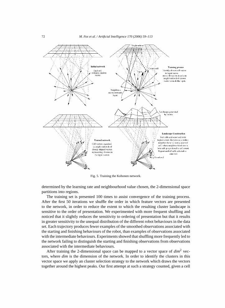
Fig. 5. Training the Kohonen network.
determined by the learning rate and neighbourhood value chosen, the 2-dimensional spacepartitions into regions.
The training set is presented 100 times to assist convergence of the training process.After the first 50 iterations we shuffle the order in which feature vectors are presentedto the network, in order to reduce the extent to which the resulting cluster landscape issensitive to the order of presentation. We experimented with more frequent shuffling andnoticed that it slightly reduces the sensitivity to ordering of presentation but that it resultsin greater sensitivity to the unequal distribution of the different robot behaviours in the dataset. Each trajectory produces fewer examples of the smoothed observations associated withthe starting and finishing behaviours of the robot, than examples of observations associatedwith the intermediate behaviours. Experiments showed that shuffling more frequently led tothe network failing to distinguish the starting and finishing observations from observationsassociated with the intermediate behaviours.
After training the 2-dimensional space can be mapped to a vector space of dim2 vec-tors, where dim is the dimension of the network. In order to identify the clusters in thisvector space we apply an cluster selection strategy to the network which draws the vectorstogether around the highest peaks. Our first attempt at such a strategy counted, given a cell
M. Fox et al. / Artificial Intelligence 170 (2006) 59–113 73
〈i, j 〉, the number of cells that were within a fixed radius (we used 0.085) of 〈i, j 〉. Thiscount was used to measure the influence of 〈i, j 〉 over the whole network. We then used ahill-climbing strategy to associate plateau cells with the first closest peak found.
There are several weaknesses associated with this approach. The first is that, using thisstrategy, the composition of the peaks ends up very sensitive to the noisiness of the cellsin the network. We noticed that, with different random initialisations, we got very differ-ent cluster landscapes. A cell might be pulled one way or the other depending on randomfactors, so that a small change in the initialisation of the network could lead to huge dif-ferences in the cluster landscape. Large variations make the later learning results highlydependent on arbitrarily chosen random numbers.
Another weakness is that the cells exerting the most influence in these terms over thenetwork are not necessarily the cells that attracted most of the input during training. Usingthis method we could end up throwing out the clusters we are really interested in favourof ones that attracted little input and are not good indicators of the behaviour of the robot.Further, by associating the cells in a plateau with the nearest peak we caused the network todistort, sometimes very badly in the cases where there are large plateaus. A better approachseems to be to restrict the amount of draw that one cell can have over another, and therebyspread the clusters more evenly over the landscape.
To address these problems we developed a different cluster selection strategy which usesthe number of inputs attracted to each cell as a way of identifying the cluster landscape.The cells that attracted the most inputs we take to be the highest peaks in the landscape.Given that the cluster landscape is intended to represent the structure in the data set wedecided that a cell that attracts very few inputs is unlikely to be interesting, so we focus ourattention on the high peaks. To achieve this focus we associate a varying neighbourhoodsize with the peaks in the network, considering the peaks in descending height order. Thisneighbourhood is different from the learning neighbourhood used during training.
We first order the peaks then, choosing the largest first, remove from the network all ofthe cells in its neighbourhood. The size of the neighbourhood is determined as �H
C�, where
H is the number of inputs attracted to the highest overall peak in the network and C isthe number of inputs attracted to the current peak. This value is used as a radius aroundthe peak cell. The process is repeated for the next highest peak until no cells remain to beconsidered.
Let C be the current peak and H be the height of the highest peak in the network.Clearly, if H
Cis large for most values of C then we risk losing the interesting structure in
the network. This is obviously undesirable, resulting in a small collection of clusters thatis unlikely to be discriminating. We require the value of H
Cto have a slow, smooth gradient
over a sufficiently large collection of discriminating clusters. For the size of our data setsufficiently large means tens of clusters. To achieve such a gradient we require the ratio ofH to C to be small for tens of Cs. By examining the cluster landscapes constructed fromour data set we confirmed that this requirement is satisfied. Fig. 6 gives an example of atypical cluster landscape generated using a network of size 30.
We have found that using this strategy we improve the clustering stability by reducingsensitivity to the noisiness of the randomly generated vectors. Peaks still move around inthe network because of the random initialisation, but this is to be expected. The experiments

74 M. Fox et al. / Artificial Intelligence 170 (2006) 59–113
Fig. 6. A clustering landscape obtained using a 30 × 30 Kohonen network.
presented in Section 6.4 show that we achieve a high degree of stability in the clusteringresults across different random number initialisations.
Following training the feature vectors are reintroduced to the network for classification.During classification, each input sequence vector is associated with the peak vector towhich it is closest according to a scalar multiplication comparison between the featurevector and each peak vector. The cells in the network that correspond to the peaks containvectors that characterize the evidence items found by the clustering process. These are theelements of the set ξ and correspond to the evidence items that can be observed by therobot as it executes its task. We refer to these vectors as characteristic vectors.
Our clustering approach is related to that of Oates et al. [15] who considered the prob-lem of clustering the experiences of a robot into qualitatively different action outcomes.Their cluster prototypes, which are closely related to our characteristic vectors, constitutean ontology of activity. It is intended that they correspond to the qualitatively differentstates in which a robot can find itself, following the execution of an action, and that theyprovide the basis for automating the description of actions at the task-planning level. Bycontrast, our characteristic vectors are interpreted as high level observations, or evidenceitems, associated with states at the intermediate level of description rather than at the task-planning level. As we will see, observations contribute to the identification of states, at thisintermediate level, which might have no interpretation for the human observer but whichmay be critical in accurately modelling the behaviour of the robot with respect to its task.
At the end of the classification phase all of the feature vectors in our data set have beenclassified with one of the characteristic vectors in the network. This puts us in a position toconstruct an observation code book.
3.1.2. Constructing the sensor modelA code book [27] is a mapping from input values to a finite collection of observation
codes. To build our code book it is necessary to associate the characteristic vectors withthe labels in L ∪ {nomark}. To facilitate this we annotate each feature vector with the labelassociated with the last observation in the sliding window from which the feature vector

M. Fox et al. / Artificial Intelligence 170 (2006) 59–113 75
was constructed. If there are no labelled observations in this sliding window the featurevector is labelled no mark.
The association of a feature vector with a label results in a new structure which we calla sequence vector. The structure of a sequence vector is defined in Definition 9.
Definition 9. A sequence vector sv = ( �fi, l) is an m-dimensional feature vector associatedwith a label, l, from the set L, taken from the last labelled observation in the sub-sequenceof the partially labelled trajectory from which �fi was constructed. If there are no labels inthe subsequence then l is the no mark label.
In the construction of our code book, the input values are sequence vectors, defined inDefinition 9, and the characteristic vectors identified during the clustering phase are used asthe codes. The mapping is defined by the classification behaviour of the Kohonen network.
Definition 10. Given a trajectory t = 〈o1, . . . , on〉, the ladder lt is the sequence 〈 �f1, . . . , �fn〉of sequence vectors constructed from trajectory t .
The sequence vector construction phase defines a mapping from trajectories to ladders,defined in Definition 10, so-called because of the way that the sequence vectors overlap ina sliding window, as shown in Fig. 3.
We can now construct the association between evidence items in ξ and the labels inL ∪ {nomark} by counting the number of sequence vectors carrying each label, the featurevectors of which were classified with each evidence item. This association can be turnedinto a probabilistic observation function in the following way. Let s0, . . . , sn be the behav-ioural states labelled by L and e0, . . . , em be the evidence items. We interpret the numberof associations in a given pair (si, ej ) as a proportion, so that the probability of seeingevidence ej in state si can be easily calculated. Let Vjsi
be the set of sequence vectorsassociated with evidence item ej that were labelled with si , and Vsi be the set of sequencevectors labelled si . Now the probability of seeing evidence ej in state si is
θi(j) = |Vjsi|
|Vsi |.
The resulting function can be interpreted as a sensor model specifying the probability ofseeing each evidence item given each state. The “sensor” is the compound sensor capableof observing the evidence items found by the clusterer. This means that when subsequentlyusing the model the robot’s raw sensor data can be processed by the construction of se-quence vectors and their classification by means of cluster :Φ → ξ .
In Section 6 we present results showing the quality of HMMs learned on the basis ofsensor models constructed in this way and not further refined by state splitting. As canbe seen from Fig. 19, the quality of the HMMs learned on this basis is often poor. Wehypothesised that the states identified by the human observer might not in fact be the statesthat are most important for distinguishing between the behaviours of the robot, and thatbetter results might be obtained by sub-dividing the human-observed labels. The labelsin L ∪ {nomark} abstract out a great deal of potentially important variation in behaviour,including the transitionary behaviour that the robot exhibits as it passes from one state

76 M. Fox et al. / Artificial Intelligence 170 (2006) 59–113
to another. To explore this hypothesis we developed the state splitting strategy, brieflydescribed in Section 2.3, which decomposes each of the original labels around the groupsof evidence items that are most strongly associated with these states according to the codebook sensor model constructed as above.
3.2. Maximal cliques
As stated in Section 2.3, the inputs to the maximal clique finding algorithm are the set oflabels L, a set of partially labelled trajectories, the set of evidence items and cluster :Φ →ξ . The output is the set of states Ψ .
In the code book multiple evidence items can be associated with the same behaviouralstate. This occurs because evidence items are not perfect discriminators between states.Sometimes, the characteristic vectors of these evidence items are separated in the vectorspace by significantly large angles. When these angles exceed 30 or 40 degrees it seemsplausible that the association of these clearly different evidence items with the same be-havioural state might indicate that a decomposition of that behavioural state into sub-statesis possible.
The idea of state-splitting around distant groups of characteristic vectors is illustratedin Figs. 7 and 8. The procedure refineθ , in Fig. 7, begins by constructing, for each labels ∈ L, a graph in which the nodes are the characteristic vectors of the evidence itemsassociated with that label in the code book θ . The edges in the graph are the angles invector space between the evidence items at the two end-points. If two vectors are lessthan a pre-determined threshold apart—for example, 40 degrees—an edge between theircorresponding nodes is added to the graph and the maximal cliques remaining in the graphare found. These steps are illustrated in lines 6 to 15 of the constructGraph procedure.
The maximal cliques contain all those evidence items within 40 degrees of one another.Each maximal clique is a subset of the characteristic vectors associated with the originallabel, suggesting a substate of the behavioural state corresponding to that label. The proce-dure refineθ shows how finding the maximal cliques leads to the construction of a refinedsensor model.
The sensor model, θ0, is constructed from the code book using the identified substates.We want to replace the original behavioural states labelled by L ∪ {nomark} with theirsubstates and to share out the association between an evidence item and a label amongst allof the substates of that label. Thus: if evidence item e had a k% association with label s,and state s has p sub-states, the quantity k% has to be shared out between the p substates.This is not just a case of dividing the k% into p equal parts—the sharing has to be done ina way that reflects the proximity of each substate to the evidence item e. To do this we needto identify the centre of mass of each sub-state and measure the distance from e to each ofthese centres of mass. We obtain the average of the characteristic vectors in a sub-state toobtain the centre of mass of that sub-state. We then take the scalar product of the resultingvector and the characteristic vector of evidence item e to obtain the proximity of e to thesubstate. Finally, each substate is given a proportion of the association between e and thelabel, depending on its proximity to e. This calculation is shown on line 39 of procedurerefineθ . Fig. 8 shows how this sharing is achieved.

M. Fox et al. / Artificial Intelligence 170 (2006) 59–113 77
1: Procedure: constructGraph(θ ,s,ξ )2: Input: code book θ , label s, evidence items ξ
3: Output: graph structure G4:5: initialise graph G6: for all cluster c in ξ do7: if assoc(θ, s, c) > 0 then8: add node for c to G9: end if
10: end for11: for all (cluster) node i in G do12: for all (cluster) node j in G do13: if angle(i,j) < THRESHOLD then14: add edge (i,j) to G15: end if16: end for17: end for18: return G19:20: Procedure: refineθ (θ ,L,ξ )21: Input: code book θ , labels L, evidence items ξ
22: Output: sensor model θ0
23:24: initialise sensor model θ0
25: for all label s in L do26: G = constructGraph(θ ,s,ξ )27: {First identify the maximal cliques in G}28: Cs = maxCliques(G)29: initialise 2d array of doubles, ds30: for all cliques clq in Cs do31: {Find the mean of clusters representing nodes in clq}32: avC = computeAverage(clq)33: for all characteristic vectors c in ξ do34: {Record distance between centre of clique and characteristic vector c}35: ds[clq][c] = scalarProduct(avC,c)36: end for37: normalise ds[clq]38: for all cluster c in ξ do39: θ0[clq][c] = assoc(θ ,s,c)/ds[clq][c]40: end for41: end for42: end for43: return θ0
Fig. 7. Pseudo code showing the state splitting procedure. For both routines, assoc(θ, s, c) is the association inthe code book θ between label s and evidence item c.

78 M. Fox et al. / Artificial Intelligence 170 (2006) 59–113
Fig. 8. The state splitting procedure.
As a result of the state splitting process the code book is rewritten in terms of thesubstates found. The number of evidence items does not change as a result of state split-ting, but the number of states increases and is determined by the structure of the vectorspace following clustering. Interestingly, the states in the refined set have no interpretationfor the human other than that they were obtained by decomposition of an original set ofhuman-observed labels. Nevertheless, some of the new states might represent interestingtransitionary states that are important for learning a good state transition function and cantherefore improve the results obtained from the EM phase.
The state collection that results from the refinement of the initial state labels is the stateset Ψ , and the sensor model, constructed using the relationship between Ψ and ξ , is thefunction θ0. The relationship defines a function, ab :Ψ → L, which maps states in Ψ tolabels in the initial collection (ab indicates an abstraction step). We also define a functionev :Ψ → Pξ which, given a state in Ψ produces the set of evidence items that constitute it.The following property holds:
∀s1, s2 ∈ Ψ · ab(s1) = ab(s2) ⇒ ev(s1) �= ev(s2)
which means that, if two states map by ab to the same label, they will not contain the sameevidence items. We can also identify a mapping from labels to sets of substates which,given a label produces the set of substates in its decomposition. We call this mappingrefine :L ∪ {nomark} → PΨ .
It must be noted that two different substates in Ψ might be composed of exactly the sameevidence items. Their association with different labels distinguishes them. However, thefact that two labels contain substates composed of identical evidence items can be taken toindicate a sharing of content between the two labels. Part of the power of the state-splitting

M. Fox et al. / Artificial Intelligence 170 (2006) 59–113 79
procedure resides in its ability to identify the shared sub-structure of abstract states, as wellas the characteristics that distinguish them. We explain in Section 6 how the recognition ofshared sub-structure can be exploited in the evaluation of the learned HMM.
The idea of decomposing and augmenting the states of a HMM has been consideredby other authors [1,16]. In particular, Koenig and Simmons’ GROW-BW algorithm allowsnew states to be added to a HMM if they are needed to account for observations made by anavigating robot. Chrisman [16] shows how dynamic partitioning of the state space of themodel can overcome the problem of perceptual aliasing that occurs when a model containstoo few states to discriminate between different observations. Stolcke and Omohundro [30]show how states can be dynamically merged to generalise a HMM. In these works theHMM starts with a collection of states that is determined a priori and is known to beinadequate to account for the observations of the system. State splitting and merging isapplied during the learning process to increase the adequacy of the state set as observationsare made.
By contrast, we propose a static state splitting strategy to be performed prior to the EMlearning process. Its purpose is to increase the information content of λ0 and thereby im-prove the quality of the learned model. Indeed, the results we present in Fig. 19, Section 6,demonstrate that the quality of models learned after state splitting is significantly higherthan is obtained when state splitting is not used.
Once the state set of the HMM is decided it is never changed—only the next-state andobservation probability distributions are affected by reestimation. The states to which thesplitting algorithm is applied are the labels in L ∪ {nomark}. Splitting allows these statesto be refined so that transitionary states emerge and structure is made accessible that wasnot apparent to the human observer. It is intended that our state splitting algorithm identifya complete (with respect to the available sensors) set of the hidden states that accounts forthe behaviour of the robot with respect to its task.
3.3. Expectation maximisation
We require a way to reestimate the parameters of the HMM, and we follow the workof Dempster et al. [25] in using the EM algorithm to perform this reestimation. Our im-plementation closely follows the presentation of HMM reestimation given in Rabiner’stutorial [5]. In this section of the paper we focus on the issues that arose for us in using EMto perform the reestimation of our initial HMM. These issues are: the initialisation of theHMM parameters and their effects on the results obtained; the need for scaling and the wayin which scaling is performed when multiple histories are used in reestimation and, finally,the use of the learned HMM to diagnose the state of the system from a given history. Inorder to be self-contained, and to clarify our contribution, we summarise the main aspectsof the EM technique.
In an EM implementation of reestimation there are two key steps: the E step, which isthe calculation of the maximum likelihood of seeing the evidence given the model so far,and the M step, which is the process of updating the model to maximize the probabilityof seeing the evidence. The E step is performed using the so-called forward-backwardalgorithm, originally described in [31,32], and very clearly presented by Rabiner.

80 M. Fox et al. / Artificial Intelligence 170 (2006) 59–113
The M step, in which the transition and sensor model components of the HMM areupdated, is affected by the scaling of the values generated by the forward-backward algo-rithm. As Rabiner discusses, scaling is necessary in the E step to avoid underflow. Withoutscaling, underflow occurs because the probability of seeing a long sequence of evidence isvery small, so as the history lengths grow the E step calculations tend to zero. It is neces-sary to demonstrate that the scaled values do not change the interpretation of the updateoperations. This is straightforward to show when a single history is used for learning, butmore subtle when multiple histories are used. In the work we describe in this paper, weused multiple histories because our data set contains multiple separate and independenttrajectories. In Appendix A we discuss how we implemented the scaling mechanism fol-lowing Rabiner’s presentation. In this section, we present the core components of the Eand M steps, showing how scaling is managed in the case of multiple histories.
3.3.1. Basic frameworkWe begin by providing here some definitions from Rabiner’s tutorial that are necessary
for our presentation. The forward and backward variables are defined below. The M stepof the EM procedure, which performs the updating of the model, is defined in terms of theforward and backward variables. Definitions 11, 12, 13, 14 and Eqs. (1) and (2) are takenfrom Rabiner’s paper.
Definition 11. Given a history h = 〈e1, e2, . . . , eT 〉, a collection of states Ψ and a modelλ = (Ψ, ξ,π, δ, θ), the forward variable αt (i) is defined to be the probability of being instate si at time t , having seen the first t elements of h, given the model λ. This is formalisedas:
αt (i) = P(e1 . . . et , qt = si | λ).
The forward variable is constructed recursively as follows:Initialisation:
α1(i) = πi.Oi(e1), 1 � i � N.
Induction:
αt+1(j) =N∑
i=t
αt (i)δ(i, j)θj (et+1), 1 � t � T − 1, 1 � j � N.
Termination:
P(h | λ) =N∑
i=1
αT (i).
Definition 12. Given a history h = 〈e1, e2, . . . , eT 〉, a collection of states Ψ and a modelλ = (Ψ, ξ,π, δ, θ), the backward variable βt (i) is defined to be the probability of seeingthe last T − t elements of h, given that the state of the system at time t is si and given themodel λ. This is formalised as
βt (i) = P(et+1 . . . eT | qt = si , λ).

M. Fox et al. / Artificial Intelligence 170 (2006) 59–113 81
The recursive construction of the backward variable is as follows:
Initialisation:
βT (i) = 1, 1 � i � N.
Induction:
βt (i) =N∑
j=1
δ(i, j)θj (et+1)βt+1(j), t = T − 1, T − 2, . . . ,1, 1 � i � N.
With these variables we can now define the transition model and sensor model updatecomponents of the M step. The prior probability distribution, π , is not reestimated if anunambiguous initial state can be identified for which the probability is 1. We assume thatthis is the case, and explain why in Section 3.3.3. We begin with the basic transition modelupdate. In the following, the primed notation δ′(i, j) and θ ′
j (k) denotes the updated valuesof δ(i, j) and θj (k) respectively.
Definition 13. The transition model component δ of λ is updated according to the followingequation:
δ′(i, j) =∑T −1
t=1 αt (i)δ(i, j)θj (et+1)βt+1(j)∑T −1
t=1 αt (i)βt (i).
Definition 13 specifies that the (i, j)th element of δ′ is given by the expected frequencyof transitions from state i to state j , divided by the expected frequency of state i. Thesensor model can be updated according to a similar rule:
Definition 14. The sensor model component θ of λ is updated by
θ ′j (k) =
∑Tt=1
s.t.et=k
αt (j)βt (j)
∑Tt=1 αt (j)βt (j)
.
Definition 14 states that the probability of observing evidence k while in state j is givenby the expected frequency of being in state j and observing evidence k, divided by theexpected frequency of being in state j .
We now turn to the scaling issue and its effect on these update equations. The t th for-ward scaling term can be defined as the likelihood of seeing the first t elements of thehistory and being in state i. This is expressed as
Ct =t∏
v=1
cv,
where cv is the normalisation term:
1∑N
.
i=1 αv(i)

82 M. Fox et al. / Artificial Intelligence 170 (2006) 59–113
The (t + 1)th backward scaling term can be defined as
Dt+1 =T∏
v=t+1
cv.
The normalisation term cv is calculated during the E step. The update equations definingδ′(i, j) and θ ′
j (k) can be rewritten to incorporate these scaling terms in the M step. Eq. (1)shows how the transition model update is modified.
δ′(i, j) =∑T −1
t=1 Ctαt (i)δ(i, j)θj (et+1)Dt+1βt+1(j)∑T −1
t=1∑N
j=1 Ctαt (i)δ(i, j)θj (et+1)Dt+1βt+1(i). (1)
The variables αt (i) and βt (i) are scaled by multiplying them by Ct and Dt respectively.The scaled forms are written using the notation α̂ and β̂ . Thus:
Ctαt (i) = α̂t (i)
and
Dtβt (i) = β̂t (i).
The sensor model update θ ′j (k) can be modified in a similar way. Rabiner shows that the
terms CtDt+1 can be expressed in a form independent of t , so that they cancel, leaving theupdate operations as shown in Definitions 13 and 14.
3.3.2. Scaling with multiple sequencesRabiner discusses the fact that, depending on the kind of HMM being learned, there
may be a need to learn using multiple histories in preference to one long sequence ofevidence. In this case, it is necessary to modify the reestimation formulas to add togetherthe individual frequencies of occurrence of each sequence. Before this sum, the expectedfrequency of transitions from i to j in sequence k must be scaled by dividing it by thelikelihood of sequence k given the model. The expected frequency of state i in sequencek must also be divided by this likelihood. If Pk is the likelihood of sequence k this canbe achieved by multiplying the contributions made by this sequence to both the numeratorand denominator by 1
Pk.
δ′(i, j) =∑K
k=11Pk
∑Tk−1t=1 αk
t (i)δ(i, j)θj (ekt+1)β
kt+1(j)
∑Kk=1
1Pk
∑T −1t=1 αk
t (i)βkt (i)
. (2)
From Rabiner we have that
CTk= 1
Pk
,
so, by writing Eq. (2) in terms of the scaled forward and backward variables we obtain:
δ′(i, j) =∑K
k=1∑Tk−1
t=1 α̂kt (i)δ(i, j)θj (e
kt+1)β̂
kt+1(j)
∑Kk=1
∑T −1t=1 α̂k
t (i)β̂kt (i)
. (3)
Eq. (3) corrects Rabiner’s equation 111, in [5], in which he erroneously leaves in place the1 terms. These should be removed as they have already been taken into account in the
Pk
M. Fox et al. / Artificial Intelligence 170 (2006) 59–113 83
scaled variables. This observation was also made by Kevin Murphy in his implementationof the HMM code in the BNT package [33].
3.3.3. Initialising the model parametersIn order to help EM to avoid converging on a local maximum that is far from a global
maximum, we try to make the initial model λ0 = (Ψ, ξ,π, δ0, θ0) as informative as pos-sible. Ψ is created by state splitting applied to the initial set of state labels, L. We splitboth the visible and subjective states, with the consequence that the visible states can besubdivided into sets of substates. This makes it difficult to ensure that the useful orderingthat exists between the visible and subjective states is maintained.
A simple way to avoid this problem is not to include the visible states in the splittingprocess. However, we wish to allow interesting sub-states of the starting and finishing be-haviours to be identified if they exist in the data. We therefore restore the ordering propertyby introducing supplementary start and end states that can be ordered before and after(respectively) all the states in Ψ .
During the state-splitting process the visible states, starting and finishing are replacedby sets of states in Ψ . We specify a supplementary start, sstart, that precedes all of the statesin Ψ that are associated (through state splitting) with the visible state labelled starting, anda supplementary end, send , that succeeds all of the states in Ψ associated with the visiblestate labelled finishing. These supplementary states are added to Ψ and allow us to defineδ0 as follows:
δ0(x, sstart) = 0, for all states x,
δ0(send, send) = 1,
δ0(send, x) = 0, for all states x �= send.
The initial probabilities of transition between the supplementary states and the other statesof the model are arranged so that transitions from the supplementary start state are associ-ated with a very high probability of entering the substates of the original visible startingstate, and transitions from the substates of the original finishing state are associated witha very high probability of entry into the supplementary end state. The probability oftransitions between all remaining pairs of states are assumed equal. The details of thisconstruction are discussed in Appendix A.
Introduction of the supplementary states slightly complicates the construction of ourinitial sensor model, θ0. We must specify the observation probability associated with eachof the supplementary states. These states, which have been artificially introduced, have noparticular association with real evidence. However, they must be associated with distribu-tions over the evidence items in such a way that they do not distort the learning process.
Our solution to this problem is to introduce a supplementary start observation and asupplementary end observation, estart and eend , and to associate, with very high probabil-ity, the supplementary states with their corresponding supplementary observations. Thesedetails are also discussed in Appendix A.
Finally, π must be extended to include the supplementary states, with a probability of 1associated with the supplementary start state.

84 M. Fox et al. / Artificial Intelligence 170 (2006) 59–113
Using the supplementary states we construct the initial model:
λ0 = (Ψ ∪ {sstart, send}, ξ ∪ {estart, eend},π, δ0, θ0).
3.3.4. Finding the best state sequenceIn order to use the learned HMM to diagnose the state of the robot given a history
〈e1, e2, . . . , en〉, we need to be able to find the optimal state sequence associated withthe history: that is, the state sequence that best explains 〈e1, e2, . . . , en〉. The Viterbialgorithm [24] is a dynamic programming algorithm that finds the best state sequence〈q1, q2, . . . , qn〉 for the given history.
The Viterbi procedure relies on a quantity
δt (i) = maxq1,q2,...,qt−1
P(q1, q2, . . . , qt = i, e1, e2, . . . , et | λ)
which corresponds to the highest probability, given the model λ, along a single path,q1, q2, . . . , qt , at time t , that accounts for the first t evidence items and ends in statei. Rabiner presents an inductive definition of δt (i) that is identical to the definition ofthe forward variable, αt (i), reported here in Definition 11, except in using maximisationover previous states instead of the summation in the inductive definition of αt (i). TheViterbi procedure must also keep track of the states along the highest probability path, soit maintains an array from which the path can be extracted at the end of the maximisationprocess.
We use the Viterbi procedure to evaluate the quality of the learned HMM. The detailsof our evaluation procedure are presented in Section 6.
4. Experimental setup
4.1. Robotics environment
Although our approach is task-independent we chose to experiment with learning amodel of a navigation task. This is a fairly complex task for behavioural modelling, whilstat the same time well-understood and therefore easily experimented with. The low levelfunctionalities comprising navigation have been thoroughly explored in mobile robotics,providing a firm foundation to support the learning process. To be performed robustly,navigation involves many different capabilities including localisation, terrain modellingand motion generation adapted to the presence of obstacles. Our approach is built on topof this level. Given the basic navigation capabilities we learn a passive model of the be-havioural states that the robot visits when navigating a certain distance in a certain class ofenvironments. We are not trying to improve the way the robot navigates, but to understandhow it navigates in order to be able to predict and explain the robot’s behaviour in futureexecutions of the navigation task.
In order to build a coherent model of the navigation action, we performed a large numberof experiments with a nomadic XR4000 platform. The software system we used was anoriginal architecture developed at LAAS [34]. The sensory-motor functions are separatelyprogrammed in functional modules, using a tool named GenoM [35].

M. Fox et al. / Artificial Intelligence 170 (2006) 59–113 85
Fig. 9. A typical environment configuration from the robot’s point of view.
We chose a particular navigation technology which is well suited to the environmentsin which our robot can manoeuvre. The technology is based on the use of odometry forlocalisation, a Sick® laser range scanner for obstacle detection, and the Nearness Diagramtechnique described in [36–38] for map building, obstacle avoidance and motion gener-ation. This technique for navigation behaves very well in highly cluttered and dynamicindoor environments. It is, of course, not well suited to every kind of environment.
We recorded 58 trajectories, each taking between 30 and 90 seconds to complete, withthe robot navigating approximately 10 metres. Our environment was unstructured, con-sisting of a cluttered open space open to human traffic. We made the environment varybetween trajectories, from sparsely to highly cluttered and very dynamic. Fig. 9 showsa typical environment configuration. The space is an open area within a busy laboratory.Obstacles are placed within the space. The picture shows the positions of the obstaclesand of the desks and walls bounding the area, according to the laser readings of the robot.The positions of the obstacles are plotted according to readings taken at different pointsalong the trajectory. The localisation technique being used by the robot is based on odom-etry which explains inaccuracies in the alignments of the obstacle positions as seen fromdifferent locations. The approximate trajectory of the robot is shown as it travels from itsstarting point to its destination in a given run. At each of the points shown the laser scan isrepresented by a collection of sectors each of which represents a segment that is devoid ofobstacles according to the laser scanner.
The state of the system was sampled at a frequency of 5 Hz. Each sampling recorded thevalues of 16 variables, including the following raw features: the coordinate position of therobot, relative to its starting position within a given coordinate system; the laser readingsindicating the positions of obstacles and their proximity to the robot; the speed at which

86 M. Fox et al. / Artificial Intelligence 170 (2006) 59–113
the robot was travelling in the x and y directions; the angular velocity of the robot and theEuclidean distance travelled since the last measurement.
The choice of variables to record and to use in the construction of feature vectors is, ofcourse, highly dependent on the task, the functional level chosen for modelling and on thesensory capacity of the executive in question. However, the methodology we have followedin the research described in this paper is not restricted to the particular task and robot wehave considered. It can be applied to the learning of different tasks, using alternative robotplatforms with different sensory capabilities.
4.2. The navigation states
In our experiment we used an a priori set of labels consisting of two visible states (thestarting and finishing states) and four subjective states (hesitation, obstacle avoidance,progress and search). The progress state is the state in which the robot is moving unen-cumbered through the environment. Hesitation is the state in which the robot is temporarilytrapped in a highly cluttered region and is unsure how to proceed. Searching represents therobot embarking on routes, which turn out to be dead ends, in its effort to find a path.Obstacle avoidance is visually distinguishable from hesitation and searching because therobot is typically making progress and then veers to avoid something in its path. We didnot identify any failure states in this experiment although it would be straightforward toinclude failing trajectories (when the robot collides with an obstacle it prematurely termi-nates its trajectory) and to identify the corresponding failure states. We make no limitingassumptions that prevent the inclusion of failure states. However, our robot very rarely col-lided with obstacles, thanks to the efficacy of its control software, so we did not gather datarepresentative of failures in our experiment.
4.3. Sensory-motor data and features
We identified eight features as important for discriminating between the behaviours ofthe robot in its execution of the navigation task. These are: distance from origin, curvilineardistance travelled over the sequence, change in heading over the sequence, total rotation,clutteredness, distance from goal, speed of travel and acceleration. These features are ob-tained by smoothing and integration over 6-second intervals of time. These are standardtechniques used in signal processing [39] so we do not describe them here.
The variables distance from origin and distance from goal are useful because they helpto discriminate between the visible states start and end. The distance from origin is calcu-lated as the Euclidean distance between the position of the robot at the start of the trajectory(its starting coordinate) and its position at the start of the fragment of the trajectory cap-tured by the feature vector. The distance to goal is calculated as the Euclidean distancebetween the position at the end of this fragment and the goal coordinate.
Curvilinear distance is a segmented approximation of the actual curvilinear distancetravelled by the robot over the fragment of the trajectory represented by the feature vector.It is estimated as the sum of the Euclidean distances travelled between successive obser-vations in the fragment. Change in heading is a measure of the magnitude of the angularchange over the fragment. A large change in heading indicates that the robot is turning fre-

M. Fox et al. / Artificial Intelligence 170 (2006) 59–113 87
quently, perhaps through large angles. This would tend to indicate that the robot is avoidingan obstacle or searching for a viable path. Total rotation measures the extent to which thechange in heading is cancelled out by turning back and forth rather than by turning pre-dominantly in one direction. Rapid oscillating is associated with hesitating and searchingbehaviours, giving rise to small angular turns the sum of which is close to zero. Cluttered-ness is a measure of the density of obstacles in the robot’s immediate vicinity over theduration of the sequence. It is a smoothed representation of the clutteredness associatedwith the individual observations in the fragment represented by the feature vector.
Speed of travel is a smoothed representation of the speed at which the robot is travellingover a fragment corresponding to a feature vector. Acceleration is a measure of the changein speed of the robot over the fragment, obtained by taking the difference between themaximum and minimum speeds at which the robot travelled over consecutive observations.If the speed is low but the acceleration is high, this would indicate that the robot is brakingoften and then speeding up again, as might occur when the robot is negotiating its wayaround obstacles.
Finding a discriminating set of features in a complex data set is a challenging problem.We experimented with various different combinations before arriving at the above collec-tion of eight features. Our choice of features was influenced by the particular task at hand:a different task would require a different set of discriminating features to characterise it.
5. Learning a hidden Markov model
The preceding sections have described the components necessary to learn a hiddenMarkov model from the raw signals emitted by a physical system. We now bring thesecomponents together into a learning process that receives the signals emitted by the robot’ssensors and outputs a learned HMM. In the rest of this paper we discuss the quality of themodels of the navigation task learned using our methodology.
However accurate its readings might be, the observations of the robot do not preciselycorrespond to the reality in which the robot was operating. The robot can observe the worldonly partially by means of its sensors. Since we are interested in knowing how the robotwill behave in reality it is necessary to make a connection between the internal world ofthe robot and the external world in which it acts and senses. We approached this problemthrough the use of a simple labelling strategy.
5.1. Labelling the feature vectors
To make a connection between the robot’s observations and the states of the HMM wedevised a method of labelling the observations with identifiers from the set L, described inSection 2. In our experiments L consisted of the six labels identified in Section 4.2, twoof which were visible and four subjective. These six labels correspond to behaviours thatthe experimentors were able to recognise and distinguish with reasonable certainty. Anyvisually distinguishable behaviours can be used for labelling. As described in Section 3.1,this a priori collection of labels is refined according to the patterns identified automaticallyin the data set during the clustering phase.

88 M. Fox et al. / Artificial Intelligence 170 (2006) 59–113
Fig. 10. A labelled trajectory.
During the robot runs, whenever the robot displayed a distinguishable behaviour we in-terrupted its recording so that it would associate the next observation with the correspond-ing label identified by the experimentor. Each trajectory is therefore partially labelled. Thislabelling process, coarse though it is, gives us a way of relating the recorded data to a sub-jective judgement of the external reality in which it was acquired. Fig. 10 shows a partiallylabelled robot trajectory.
The experimentor tended to introduce a slight delay into the labelling because of takingtime to recognise the behaviour being displayed. Thus, labels tend to occur slightly later inthe trajectories than the points at which the associated behaviours really occurred. This canbe taken into account in the interpretation of the labelled trajectories, as we explain in Sec-tion 6. The subjective nature of the judgements made by the experimentor of course meansthat these judgements do not precisely correspond to reality. We discuss the consequencesof this, for evaluation of the learned model, in Section 6.
It is important to emphasise that the labels play no role at all in the clustering of thedata. The clusterer is concerned only with the feature vectors and ignores the labels in boththe training and classification processes. The labels are used when clustering is complete,in the construction of the sensor model, as described in Section 3.1.2.
It would of course be surprising if human observers could select a collection of hid-den states that turned out by chance to be the most useful ones for learning an accuratenext-state transition function. We believe that the state-splitting technique we describe inSection 3.2 helps to mitigate the effects of choosing an a priori label set by introducingmissing states that are important in determining the behaviour of the robot but are notnecessarily susceptible to interpretation by the human observer.
5.2. Constructing the evidence sequence
The EM algorithm learns to improve a given initial model with respect to the evidencethat was observed by the signal source (in this case, the robot). Evidence can be presentedin a single sequence, or in multiple sequences, depending on the properties of the model.Our experiments were divided into separate trajectories of the robot, each one terminatingwhen the robot reached its goal position. Because of the structure of a trajectory one ofthe properties of the model is that it is not fully ergodic—the robot always progresses fromits start state towards its end state. We therefore chose to present the evidence as a set ofseparate histories, each one derived from a different trajectory. This presentation excludestransitions from the end state into the start state, so enables us to construct δ0 as defined inSection 3.3.3.

M. Fox et al. / Artificial Intelligence 170 (2006) 59–113 89
Each history, ht , is derived from the ladder, lt , obtained by sequence vector constructionfrom a given trajectory t . Our strategy is to build a sparse ladder, slt , by taking everykth sequence vector from lt , where k is a density value determined experimentally. Forexample, if k = 1 then slt will be identical to lt , whilst if k = 15 then slt will be a thinnedversion of lt containing every 15th step in lt .
Following construction of slt each of the feature vectors obtained from the sequencevectors in slt are presented to the Kohonen network for classification. Thus, each step �fk
in slt is classified with an evidence item ξsltk, so that the sparse ladder slt = 〈 �f1, . . . , �fn〉
produces a history ht = 〈ξslt1, . . . , ξsltn 〉 of evidence associated with the trajectory t .
We would expect the quality of the learning to improve as the frequency k increases.When evidence is sampled at a low frequency much of the robot’s behaviour is omittedfrom the history and the association between the evidence items sampled and the observedbehaviour is likely to be missed. With higher frequencies the history is richer and thisassociation is more likely to be found. The results we present in Section 6 show that indeed,up to some point, higher frequencies result in better models being learned.
Fig. 11 shows an example of a learned HMM where the evidence was sampled at 0.6 sec-ond intervals. The picture shows that the state-splitting process produces 65 states from theinitial set of 7 labels (including the no mark label). To simplify interpretation of the graph,states are grouped into rectangles associated with the labels they refine. Dark transitionsrepresent the highest probability transitions between states whilst lighter edges representlower probability transitions.
5.3. Parameter settings
Before discussing the results we explain how we chose the values of the parameters thatgovern important aspects of the clustering and learning processes.
When decomposing the initial set of labels, L∪{nomark}, using the evidence items in ξ ,it is necessary to decide which characteristic vectors should participate in the decomposi-tion of each label. For each label l ∈ L∪{nomark} we used a fixed threshold of associationbetween the characteristic vectors and that label to determine which vectors to partitioninto the substates of the label. The association of a characteristic vector, c, with a label, l,is given by the number of sequence vectors labelled with l that were classified with c afterthe network training process. The reason for setting a threshold is that some characteristicvectors turn out to be very marginally associated with some labels. There can be one or twoorders of magnitude difference between a low association and the mean for a given label.We judged that low associations can be the consequence of noise effects in the trainingprocess.
The threshold was defined as
ml = µl − σl/4,
where µl is the mean association between the characteristic vectors and l, and σl is thestandard deviation of the association. Experiments showed that using the mean associationas the threshold led to too many vectors being excluded from the decomposition of thelabel, and improved results were obtained by lowering the threshold slightly. We achieved

90 M. Fox et al. / Artificial Intelligence 170 (2006) 59–113
Fig. 11. A learned HMM for the navigation task. The rectangles (which are all tall and narrow) are labelled withthe high level labels associated with the collections of states inside them. The Initial and End states are the dummystates used to construct θ0.
good results by subtracting σ/4. Our goal is to lower the threshold just enough to increaserobustness to noise in the training and classification processes.
Having selected a group of characteristic vectors to partition into the substates of a labelwe then need to decide on the degree of separation between substates. We used an angularseparation of 40 degrees to determine whether two vectors could be considered part ofthe same substate. A larger angle than this causes the substates to fragment and destroysthe structure of the label. Too small an angle results in large substates and inadequatedecomposition. The importance of this parameter was discussed in Section 3.2.
To construct the evidence histories we took every third sequence vector from the collec-tions of sequence vectors generated from the 58 trajectories in our data set. We consideredlower frequencies, and we present comparative results in the next section. Because obser-vations were sampled at 5 Hz, selecting every third vector corresponds to taking evidenceevery 0.6 seconds along the trajectory.

M. Fox et al. / Artificial Intelligence 170 (2006) 59–113 91
6. Results and discussion
We present analyses of two sets of results. We first consider the quality of the learnedHMM in terms of its ability to produce traces through the abstract state space that corre-spond to those that the robot was observed to follow in reality. The quality of the HMM ishighly dependent on the clustering phase. As a second stage in our evaluation we thereforeexamine the stability of the clustering results.
The clustering process is mainly affected by two parameters: the size of the networkand its random initialisation. As noted in Section 3.1, the results of the clustering phaseare also slightly sensitive to the order of presentation of the training data, but we do notdiscuss this issue further. We experimented with a range of different network sizes andnoted how these affect the quality of the traces produced by the consequent learned HMM.In the discussion below we present the results obtained using a network of size 30. InAppendix B we present an evaluation of HMMs learned using networks of different sizes.We found that the clustering results can be sensitive to the random initialisation, leading tovarying sized sets ξ and Ψ . We therefore average our results for a given network size over20 different random initialisations of the network.
6.1. Evaluation of the HMM
The Viterbi algorithm provides a way of diagnosing the behaviour of the robot from theobservations it makes in the execution of its task. Given the histories of evidence itemsconstructed during the clustering process, and the learned state transition and sensor mod-els, we can diagnose the most probable state transitions of the robot by finding the mostprobable explanation for each evidence item given the states it visited so far.
One way to evaluate the quality of the learned HMM is to compare the sequences ofstates constructed by the Viterbi algorithm with those that the human observed the robotvisiting during its execution of the task. We refer to a sequence of states visited by theViterbi algorithm as a Viterbi sequence, and to the states along such a sequence as theViterbi states. The human observer drew observations from the set of visible and subjectivestates, L, defined in Section 2.
The only way we have of identifying the states actually visited by the robot in a giventrajectory is to use the labelled observations in that trajectory. The labelling process wasinaccurate because of the difficulty, for the human observer, of distinguishing between sim-ilar states of the robot (for example, between hesitation and searching). Furthermore, thehuman observer tended to label late because it took time to interpret the robot’s behav-iour and select the most appropriate label. This means that the label often ended up beingassociated with data recorded after the robot had already transitioned to a different state.Finally, there were fewer sequence vectors in the data set labelled with visible states thanlabelled with subjective states, because the robot entered the visible states less frequently.The learning process was therefore slightly biased against recognising the starting and fin-ishing behaviours as distinct from the other behaviours in the model. However, althoughthe labelling process was flawed, the labels do provide us with a way to connect the Viterbisequences with an observed (though somewhat noisy) reality.

92 M. Fox et al. / Artificial Intelligence 170 (2006) 59–113
We evaluate a given Viterbi sequence V by comparing it with the labelled trajectory itcorresponds to. The states in V are separated by k/r seconds, where k is the frequencywith which the sequence vectors are sampled from the trajectories in the construction ofthe histories and r is the rate (in Hz) at which observations were sampled by the robot. Thechosen frequency determines the density of evidence items in the histories. The Viterbisequence V is obtained from a given history, H , and there is exactly one Viterbi statein V for every evidence item in H . For each history we record the trail of Viterbi statescorresponding to the evidence items and then super-impose the human-observed labels atthe times along these trails at which they occur in the underlying trajectory. We define theassociation between a history and a trail as follows.
Definition 15. A trail, T = 〈t1, . . . , th〉 is a sequence of Viterbi states corresponding to ahistory H of h evidence items. For each evidence item in H there is exactly one Viterbistate in T .
Definition 16. A labelled trail is a trail on which human-observed labels have been super-imposed. These labels do not necessarily coincide with states on the trail.
Definition 17. The trail fragment preceding label l in a labelled trail is the sequence ofViterbi states, V = 〈vk, . . . , vm〉, intervening between the last human-observed label beforel on the trail, and l. If l is not coincident with vm then we add to the fragment the Viterbistate, vm+1, immediately following l.
As Definition 17 shows, the trail fragment preceding a label l can actually contain thefirst Viterbi state following l on the trail. The reason for this is that, if l lies betweentwo Viterbi states, it might correspond to the Viterbi state on either side of it. The humanlabelling process was not sufficiently reactive for this possibility to be ruled out.
We increment the score for a trail each time there is a match between the human-observed label and the preceding trail fragment. The super-imposition of human-observedlabels along the trail, and the association between the label and the preceding trail frag-ment, can be seen in Fig. 12.
Care has to be taken in defining what is meant by a match. Because of the problem of latelabelling, discussed in Section 5.1, we look in the preceding trail fragment for a substatethat is identical in structure to any one of the substates comprising label l. Definition 19states this precisely.
Fig. 12. The structure of a trail.

M. Fox et al. / Artificial Intelligence 170 (2006) 59–113 93
Definition 18. Two states si and sj in Ψ are ξ -identical if they contain exactly the sameelements of ξ .
Definition 19. A human-observed label l ∈ L is associated with a set of substates S ={s1, . . . , sm} by means of the mapping refine :L → PΨ . We say that l matches its precedingtrail fragment V if at least one of the substates in V is ξ -identical to one in the set S.
Given that the preceding trail fragment might be long, Definition 19 might seem over-permissive. It suggests that the scoring rate for poor Viterbi sequences could be artificiallyincreased because, in a long preceding trail fragment, the likelihood of seeing a matchingsub-state seems high. This might be the case if preceding trail fragments tended to ex-hibit much fluctuation between states at the level of the human-observed labels. However,Fig. 13 shows that, across all the network sizes we used, the preceding trail fragments arehighly stable at this granularity despite the occurrence of many subtle state changes at thegranularity of the sub-states.
We compared the fluctuation between Viterbi states within a trail fragment, and betweenthe corresponding interpretations of those states under the application of ab :Ψ → L. InFig. 13 the rows correspond to different sizes of clustering network. The columns describethe degree of state variation observed in the trail fragments generated by the Viterbi algo-rithm using a model learned on the bases of these networks.
Variation is measured by counting how many times the value changes within each trailfragment. The final columns show the mean variability ratio, substates to labels, as a per-centage, and its standard deviation. It can be observed that, in a network of size 30, thereis three times more variation at the substate level than at the label level, and this picture isfairly consistent across the different network sizes. Furthermore, the variability within thelabel level is very low (consistently less than one state change). We find these results veryencouraging, because one would expect, in a rational system, to see more significant statechange at fine levels of granularity, with stability increasing as the granularity increases.
6.2. Precision measurements
Analysis of the relationship between substates and labels demonstrates that the samesubstate can be associated with multiple labels, revealing some confusion in the model’sability to distinguish similar behaviours.
Consider a substate, s, that is shared between k different labels. During the evaluationof a Viterbi sequence the score will be incremented if the human observed any one of
Label variability Substate variability Variability ratios
Mean Std Mean Std Mean (%) Std (%)
15 0.82 0.29 1.81 0.60 229 6020 0.80 0.30 1.96 0.69 255 7325 0.81 0.29 2.13 0.74 274 8230 0.79 0.28 2.20 0.75 295 9635 0.78 0.27 2.28 0.77 307 86
Fig. 13. Table showing state fluctuation within trail fragments.

94 M. Fox et al. / Artificial Intelligence 170 (2006) 59–113
the k labels and the Viterbi sequence visited s during the preceding trail fragment. Theusefulness of this evaluation depends on k being as close to 1 as possible.
We observed that in the case where a substate maps to 4 or more labels, it can addpoints to the evaluation almost regardless of the label applied by the human observer. Thismakes such a substate almost completely undiscriminating, artificially inflating the corre-spondence between the Viterbi sequences and the label sequences. This led us to devise amethod for measuring the degree of precision of the ab :Ψ → L mapping.
The measure is obtained by calculating, for each substate, the number, n, of labels withwhich it is associated. This number is used to give the number of pairwise comparisonsfrom which Viterbi sequences containing this substate could benefit. We sum this valueover all of the m substates, giving the following quantity:
m∑
i=0
ni ∗ (ni − 1).
This quantity is then divided by the total number of substate pairs:∑m
i=0 ni ∗ (ni − 1)
m ∗ (m − 1)
resulting in the proportion of all possible comparisons from which a Viterbi sequence couldbenefit undeservedly from visiting the substate. The higher this value the lower the preci-sion of the mapping. We call this value the confusion factor.
As can be observed from the comparison presented in Appendix B, the confusion factoris highest in small networks. This can be explained because small clustering networkslead to few distinct characteristic vectors, so that state-splitting results in a high degree ofsharing of vectors across states.
6.3. Results
Fig. 14 shows the Viterbi sequence evaluations obtained from a HMM learned on thebasis of 20 randomly initialised networks of size 30. The results are presented as a dis-tribution over the 58 trajectories and the 20 random numbers (1160 values). The meanscore was 76.18%, which is very promising. However, because of the precision issue wemust take into account the extent of confusion exhibited by the model. A high degree ofconfusion would undermine this apparently high score. In order to evaluate how good thescore really is we must also take into account the consistency of agreement between theViterbi sequences generated using different random number seeds. Low consistency (indi-cating that the quality of the HMM is sensitive to the random initialisation of the clusteringnetwork) would also undermine the goodness of the score.
Fig. 15 shows the benefit, as a percentage of overall score, obtained from confusionresulting from a network of size 30. The rows of the table correspond to the human-observed labels, while the columns correspond to states in L ∪ {nomark} obtained byapplying ab :Ψ → L to the winning states in the preceding trail fragments of the Viterbisequences (the Viterbi state that wins in a comparison is the one that is responsible forincrementing the score on that comparison). We denote the no mark state using NM. Thisstate was never observed by the experimentor but could be identified as the most probable
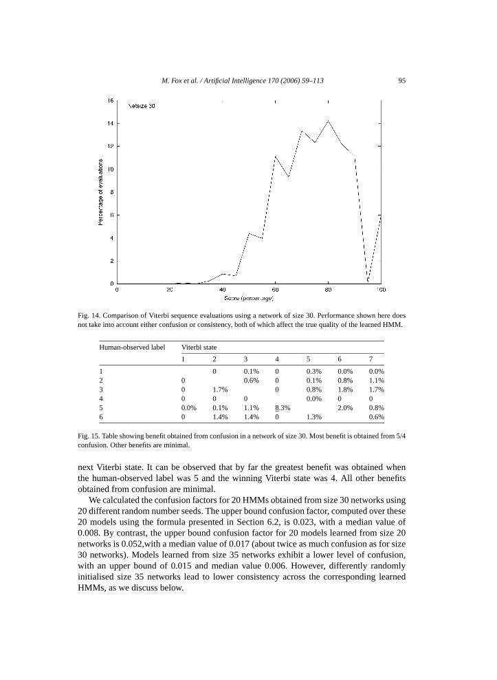
M. Fox et al. / Artificial Intelligence 170 (2006) 59–113 95
Fig. 14. Comparison of Viterbi sequence evaluations using a network of size 30. Performance shown here doesnot take into account either confusion or consistency, both of which affect the true quality of the learned HMM.
Human-observed label Viterbi state
1 2 3 4 5 6 7
1 0 0.1% 0 0.3% 0.0% 0.0%2 0 0.6% 0 0.1% 0.8% 1.1%3 0 1.7% 0 0.8% 1.8% 1.7%4 0 0 0 0.0% 0 05 0.0% 0.1% 1.1% 8.3% 2.0% 0.8%6 0 1.4% 1.4% 0 1.3% 0.6%
Fig. 15. Table showing benefit obtained from confusion in a network of size 30. Most benefit is obtained from 5/4confusion. Other benefits are minimal.
next Viterbi state. It can be observed that by far the greatest benefit was obtained whenthe human-observed label was 5 and the winning Viterbi state was 4. All other benefitsobtained from confusion are minimal.
We calculated the confusion factors for 20 HMMs obtained from size 30 networks using20 different random number seeds. The upper bound confusion factor, computed over these20 models using the formula presented in Section 6.2, is 0.023, with a median value of0.008. By contrast, the upper bound confusion factor for 20 models learned from size 20networks is 0.052,with a median value of 0.017 (about twice as much confusion as for size30 networks). Models learned from size 35 networks exhibit a lower level of confusion,with an upper bound of 0.015 and median value 0.006. However, differently randomlyinitialised size 35 networks lead to lower consistency across the corresponding learnedHMMs, as we discuss below.

96 M. Fox et al. / Artificial Intelligence 170 (2006) 59–113
The high degree of 5/4 confusion can be explained in the following way. The label 4corresponds to the finishing state and the robot normally entered the finishing state im-mediately after visiting the state labelled 5. Thus, sequence vectors labelled 5 have manyfeatures in common with those labelled 4, causing the clusterer to confuse the correspond-ing observations. A sequence vector labelled 5 is therefore likely to be classified with anevidence item associated with a substate of state 4. This is occurring when the Viterbi se-quence proposes a 4 when the human-observed label was a 5. This confusion very rarelyoccurs the other way around because δ0 is a Bakis model [40] (a partially ordered model)which strongly reinforces the recognition of the terminal state.
For a given network size and trajectory, consistency is a measure of the agreementbetween the Viterbi sequences generated for that trajectory over the 20 different randomnumbers. Clearly, the most reliable performance is obtained when confusion is low andconsistency is high. We obtained the best combination of these factors using a networkof size 30. Fig. 16 shows the consistency obtained using 20 size 30 networks. This graphdepicts the mean percentage of the Viterbi sequences that agree on each state visited alongeach of the 58 trajectories. It shows that the highest degree of consistency reached is 92%,whilst the models demonstrated at least 77% consistency on 90% of the trajectories.
The frequency at which evidence items are sampled from the data significantly af-fects the quality of the learned HMM, according to our evaluation. Fig. 17 shows thatperformance quickly declines as the frequency decreases, consistent with the hypothesisproposed in Section 5.2.
Fig. 16. Consistency of agreement between Viterbi sequences for models based on networks of size 30. Thex-axis shows the percentage of agreement obtained. The y-axis shows the cumulative percentage of trajectoriesbounded by the corresponding degree of consistency.

M. Fox et al. / Artificial Intelligence 170 (2006) 59–113 97
Fig. 17. Comparisons of Viterbi sequence evaluations using different evidence frequencies. The frequency numberindicates the separation of successive sequence vectors, in 1
5 seconds, since the raw data is sampled at 5 Hz. Thus,a large frequency number corresponds to a lower frequency of evidence sampling. Lower frequencies lead to adegradation in performance.
We performed an experiment to determine whether the construction of the initial sensormodel using the code book approach gives any advantages over using a random initialsensor model. Fig. 18 shows that a clear advantage is obtained. We also tested the advantageobtained from state-splitting, by comparing the results obtained using state splitting withthose obtained from the initial set of user-supplied labels only. Fig. 19 allows us to concludethat state-splitting yields a highly significant advantage.
6.4. Evaluation of the clustering phase
We focus our discussion on the stability of the clustering results we obtained for a givennetwork size. Different random initialisation led to a marked difference in the sizes of thesets ξ and Ψ . We have already seen (in Fig. 16) that the differences observed in the sizes ofξ and of Ψ do not lead to a consequent divergence in the behaviour of the learned models.We now show that the cluster structures are stable despite the variation in the sizes of theξ s constructed using different random initialisations.
In the table in Fig. 20 we show the extent to which the identity of states in L is preservedacross different random initialisations. We require the following definitions.
Definition 20. The weight of an element s ∈ Ψ is computed as the sum of the associationsbetween s and each element e ∈ ξ such that e ∈ ev(s). The association is determined by thecell (s, e) in the matrix defined by θ0. We denote the weight of s by ωs .

98 M. Fox et al. / Artificial Intelligence 170 (2006) 59–113
Fig. 18. Comparing random initial sensor model with a code book generated after Kohonen network clustering.Random initial sensor models lead to highly significantly poorer performance than the code book sensor models.
Fig. 19. Comparing the results using state-splitting with results obtained not using splitting.

M. Fox et al. / Artificial Intelligence 170 (2006) 59–113 99
Net size 30
Label 1 2 3 4 5 6 NM
1 66.28 0.59 0.53 0 19.44 6.4 6.762 0.5 36.18 8.23 0.29 0.28 21.18 33.343 0.89 5.49 30.49 0.05 6.04 35.96 21.084 0 0.37 0.11 50.8 45.77 0.44 2.515 14.65 0.13 2.35 25.57 46.82 2.93 7.546 3.81 7.55 13.95 0.24 2.89 59.07 12.48NM 3.4 12.86 8.66 0.57 7.86 13.12 53.53
Fig. 20. Table showing strength of identity of states in L across random initialisations of the clustering network.Values are percentages. We consider confusion with the no mark state, NM, not to be problematic.
Definition 21. The combined weight of an element l ∈ L is computed as the sum of theweights ωs of each element s in refine(l).
We now define a measure of association between two substates drawn from differentstate sets, Ψ1 and Ψ2.
Definition 22. The association product of two substates s1 ∈ Ψ1 and s2 ∈ Ψ2 is computedas the product of the combined weights of the labels, l1 and l2, obtained by abΨ1(s1) andabΨ2(s2) respectively.
Definition 23. The centre point of a substate s ∈ Ψ is computed as the average of theevidence items in ev(s). We denote the centre point by cps .
To measure the degree of preservation of identity of states in L we construct a squarematrix in which each cell (i, j) indicates the extent to which is and j s coincided acrossrandom initialisations of the cluster network. The matrix indicates that states in L preservetheir identity well if the values along the diagonal are high (preferably the highest valuesin each row).
Given two collections of substates, ΨA and ΨB , computed using different random num-ber seeds A and B , we first compute the centre points of the elements in the two collections.We then sample a centre point, cpsA
, from ΨA and measure its closeness to each of the cen-tre points computed in ΨB . The closest centre point in ΨB is denoted cps′
B. The matrix
entry for (s, s′) is increased by the association product of s and s′. The results of ouranalysis are shown in the table in Fig. 20, where it can be observed that the values alongthe diagonal are indeed the highest, except in the case of label 3 where there is significantconfusion with label 6. The table shows the percentages of the associations within eachrow attaching to each label. We include the no mark label, which we denote NM. Someconfusion between certain pairs of states, such as 3 and 6, is evident, as we observed inour discussions of confusion in Section 6.1. Nevertheless, the results overall indicate thatvariation in the number of evidence items and substates constructed by the clusterer, acrossdifferent random initialisations, does not translate into instability in the recognition of thekey behavioural states.

100 M. Fox et al. / Artificial Intelligence 170 (2006) 59–113
7. Future work
In our future work we intend to use the learned HMMs for monitoring and controllingthe execution of the corresponding tasks. We are developing a plan execution architecturein which the learned HMMs provide a low level state estimation capability that supports themonitoring of the execution of a specific planned action (or task). As the robot is executinga task the Viterbi algorithm can be used on-line to track the most likely trajectory followedby the robot and to provide a detailed picture of how the execution path is likely to unfold.The key advantage is that the HMM allows failure to be predicted before it occurs, enablingan appropriate response such as the early termination of activity.
Fig. 21 shows part of the architecture of a plan or policy execution system that usesthe learned HMMs for monitoring and controlling the execution of dispatched actions. Atits simplest, controlling the execution of a task could be limited to aborting its executionwhen the probability of failure is predicted to be above a given threshold. The componentof the architecture labelled state estimation is the component that tracks the traversal of thecurrent HMM(s) and reports the behavioural state of the robot to the execution monitor atregular intervals. On each state report the monitor sends a command to the execution sub-system to either abort the task execution or to continue following the low level programassociated with the task (this could be a hand-programmed control strategy or a policy,whatever was the low level control strategy being followed by the robot when the HMMwas learned). When the reported state is one of the terminal states of the task, the executionmonitor reports the task as having been successfully completed and the HMM correspond-ing to the next dispatched action is accessed.
The relationship between the monitor and the state estimation component is inspiredby the model-based diagnosis work of Williams and his co-authors [21,41]. These tech-niques underpin the plan execution and monitoring capability of the Remote Agent [42]which remains one of the most prominent and successful applications of plan execution
Fig. 21. A plan execution architecture using behavioural state monitoring. When an action is dispatched for exe-cution, the corresponding learned model is dispatched to the state estimation module to allow behaviour tracking.The heavy line in the model suggests the most probable trajectory being followed. There is feedback from thestate estimation to the execution monitor and dispatcher to communicate successful termination of a task or itsprobable failure.
M. Fox et al. / Artificial Intelligence 170 (2006) 59–113 101
technology. Livingstone, the model-based reasoning component of Remote Agent, is a dis-crete model-based controller using a single declarative spacecraft model to detect failuresduring the execution of planned steps and propose strategies for the repair or replacementof failed components. In our work the models are behavioural rather than physical anddiagnosis identifies deviant behaviour rather than disfunctional system components. Oncerecognised, deviant behaviour can be terminated to avoid either task failure or the unnec-essary waste of resources committed to a failing endeavour.
We have taken care in this paper to show that our work with the navigation task isnot specific to any particular robot platform or environmental setup (although the learnedmodel is dependent on these factors). To explore the generality of our approach we havebegun to consider other tasks belonging to other application areas. In particular, we havesuccessfully applied the whole learning process to learning models of both navigation andsimulated science-gathering actions on a different robot platform.
8. Conclusions
We have shown that stochastic learning techniques from signal processing can be usedto learn a hidden Markov model of a robot’s behaviour as it executes a given task. Themodel provides an introspective capability which can be integrated with high level missionplanning and reasoning. The learning of this model can be completely automated fromthe point of acquisition of sensor readings by the robot. Although we have presented ourwork in terms of the specific task of indoor navigation, using a specific robot platform,our approach can be generalised to different tasks and platforms. We make no assumptionsabout the sensory-motor equipment of the robot. The initial clustering phase is completelygeneral, resulting in the organisation of the raw sensor readings into a discretized collec-tion of codes. The codes are taken to be abstractions of the robot’s observations, sensedby means of an abstract sensor as described by a code-book based sensor model. A prob-abilistic state transition model is then learned, together with a refined sensor model, usingthe Expectation Maximization algorithm.
Although EM has been used before to learn models of behaviour, we have made severalinnovations. First, we do not define the state set in advance, but leave this to be deter-mined following the clustering phase. Thus, the number of states in the transition modelis determined dynamically and the human makes few prejudgements about the nature ofthe behavioural model. Second, the states in our model correspond to substates of thebehaviours, such as hesitation, obstacle avoidance and search, of the robot, rather thanconfigurations of the robot with respect to physical features of its environment. Thus, thelearned HMM is a model of how the robot behaves, which applies equally well in anyphysical environment sharing the same structural features as the ones in which learningtook place.
We have so far evaluated the learned HMMs by using the Viterbi algorithm to explainhistories of evidence obtained by classification of the observations recorded by the robotduring executions of its task. We compared the Viterbi sequences generated with the labelsapplied by the human observer to the robot observations. These labels provide a connectionwith reality which, although not perfect, allows us to estimate the extent to which the

102 M. Fox et al. / Artificial Intelligence 170 (2006) 59–113
learned HMM accounts for the uncertainty in the actual execution environment. Our nextstep is to evaluate the learned HMMs by using them as the basis of an execution monitoringstrategy on-board the robot. Much remains to be done, but we believe we have made animportant first step towards learning a reliable connection between the raw sensed datarecorded by a robot and a symbolic reasoning level.
Acknowledgements
We would like to thank Felix Ingrand, Derik Schröter, Brian Williams and NicolaMuscettola for helpful discussions and suggestions. We are grateful to Jonathan Gough forhelping to explore the generality of our approach by considering its application to learningmodels of different tasks. We would like to thank the anonymous reviewers for their ob-servations and suggestions. Finally, Maria Fox wishes to thank the CNRS for funding thesabbatical visit to LAAS that made this work possible.
Appendix A. Implementation
A.1. Implementing the scaling and reestimation mechanism
As described in Section 3.3.1, the forward and backward variables αt (i) and βt (i) arescaled using the scaling coefficient
ct = 1∑N
i=1 αt (i).
Thus, the same term is used for scaling βt (i) as is used for normalising αt (i), so a simplestrategy is to collect the normalisation terms that are computed during the forward compu-tation and use them to scale the backward variables during the backward computation.
To reestimate the δ component of the model we simply calculate the sum, over all timest , of the expected frequency of transitions from any state i into any state j , divided by thesum, over all times t , of the expected frequency of transitions from state i. The accumu-lation of the first sum is performed by line 15 and the second by line 10 of the procedureupdateδ in Fig. A.3. The division is computed by line 6 of procedure doδupdate in Fig. A.5.
A similar update function can be defined for θ , which calculates the expected frequencyof being in a state i while observing evidence e, divided by the expected frequency of beingin state i. These functions implement the equations presented in Definitions 13 and 14.When multiple histories are used the situation is complicated by the need to calculate thesefrequencies independently for the different histories.
In Fig. A.1 we show the reestimation mechanism that is typically presented for singlehistories of evidence. Fig. A.2 contrasts this with the multiple histories case.
To implement the equation shown in Section 3.3.2 we distinguish between the local andglobal frequencies of occurrence. For the transition model update function this requires asquare matrix and a vector to be defined for each history hk : Fijk
(the local frequencies ofany i, j transitions) and Fik (the local frequencies of transitions from any state i). A globalmatrix, Fij , must also be defined, together with a global vector Fi . The dimensions of allthese structures are determined by the number of states in δ.

M. Fox et al. / Artificial Intelligence 170 (2006) 59–113 103
1: Procedure: reEstimate(M,h,P)2: Input: model M, single history h of T evidence items, prior state distribution P3: Output: updated model M4: repeat5 {forwardBackward returns the array of T state distributions, sv}6: {Note that forwardBackward also initialises the α and β terms used in updateδ}7: sv = forwardBackward(h,P)8: (Fi,Fij ,Fi) = updateδ(M,h,sv)9: CFij = updateθ (M,h,sv)
10: M = doδupdate(M,Fij ,Fi )11: M = doθupdate(M,CFij ,Fi )12: until convergence13: return M
Fig. A.1. The reestimation function for the single history case. The array Fi is the expected frequency over T − 1timepoints of transitioning from each state i. Fij is the expected frequency of transitioning from a state i to a
state j . Fi is the expected frequency over all T time points of transitioning from each state i. The array CFij isthe expected frequency of being in state i observing evidence j .
For each history hk the values of Fijkand Fik are calculated within the same local
update procedure as used for the single history case, shown in Fig. A.3. These are thensummed into Fij and Fi at the end of each iteration (lines 13 and 16 in Fig. A.2). Thedivision of each Fij by Fi takes place when this summation is complete, as can be seen byexamination of the equation in Section 3.3.2. This is implemented by line 6 of Fig. A.5,as in the single history case. Finally, after each iteration of the reestimate procedure weupdate δ and θ (lines 26 and 27 of Fig. A.2) and then reset the local and global matricesand vectors to zero.
The sensor model θ is updated in a similar way. Given a history hk , the matrix CFijk
stores the local frequencies with which evidence items j are seen in states i. These valuesare summed into the global matrix CFij on line 22 of Fig. A.2. On line 17 of doθupdate(Fig. A.5) it can be seen that each CFij is divided by a further array, Fi , and not by Fi
as in doδupdate. The reason is that Fi does not store the expected frequency of exitingthe T th state because no transitions from the T th state are possible. However, evidencecan be observed in the T th state, so the correct updating of θ relies upon the divisionof CFij by the expected frequency of transitions accumulated from all timepoints. Wetherefore accumulate the values of this array in line 14 of the reEstimate procedure shownin Fig. A.2. The need to construct this additional array, storing this one additional value,applies whether single or multiple histories are used.
Fig. A.2 and its auxilliary procedures correctly implement Rabiner’s scaling and rees-timation mechanism for the case where multiple evidence sequences are presented to theEM procedure.
A.2. Dealing with split starting and finish states
When it is known that a process is characterised by distinct start and end states thebest estimation of the underlying HMM can be obtained using a left-right [5], model. In

104 M. Fox et al. / Artificial Intelligence 170 (2006) 59–113
1: Procedure: reEstimate(M,H,P)2: Input: model M, set of histories H, prior state distribution P3: Output: updated model M4: initialise Fi [], Fi [], Fij [][], CFij [][]5: repeat6: reset Fi
7: reset Fij
8: reset CFij
9: for all h in H do10: sv = forwardBackward(h,P)11: (Fih,Fijh
,Fih ) = updateδ(M,h,sv)12: for i = 0..NUMSTATES-1 do13: Fi [i] += Fih [i]14: Fi [i] += Fih [i]15: for j = 0..NUMSTATES-1 do16: Fij [i][j] += Fijh
[i][j]17: end for18: end for19: CFijh
= updateθ (M,h,sv)20: for i = 0..NUMSTATES-1 do21: for j = 0..NUMOBS-1 do22: CFij [i][j] += CFijh
[i][j]23: end for24: end for25: end for26: M = doδupdate(M,Fij ,Fi )27: M = doθupdate(M,CFij ,Fi )28: until convergence29: return M
Fig. A.2. The modified reestimation function for the multiple history case. The array Fihis the expected frequency
of transitioning from each state i calculated in the local context of history h. Fijhis the expected frequency of
transitioning from i to j in the context of h. CFijhis the expected frequency of being in state i seeing evidence
j , calculated in the context of h.
such a model there is an ordering on the states that excludes certain state transitions. If theestimation process begins by knowing this ordering it can converge on a better estimationof the state transition function, with a higher log likelihood, than is possible if it beginswith an equal probabilities transition model and prior state distribution.
In our experiments the robot always begins a trajectory in its starting position, and itends the trajectory as soon as it judges itself to be within a given tolerance of the goalcoordinate. Having ended the trajectory it never enters other states. It is impossible for therobot to enter the starting state from any other state. Therefore, there is an ordering imposedon the states: the starting state is always visited before any other state, and the finishingstate is always visited after any other state. The other states are not ordered, so the modelis not a strictly left-right model. If we fix the state collection in advance, and identify thestarting and finishing states, we can enforce the ordering that exists by initialising the EM

M. Fox et al. / Artificial Intelligence 170 (2006) 59–113 105
1: Procedure: updateδ(M,h,sv)2: Input: model M, single history h of T evidence items, array of state distributions sv3: Output: triple containing:4: array of expected number of transitions from each state (Fi )5: array of expected number of transitions between state pairs (Fij ) and6: array of expected number of times in each state (Fi )7: initialise Fij [][], Fi [], Fi []8: for i = 0..NUMSTATES-1 do9: for t in 0..T-2 do
10: Fi [i] += sv[t][i]11: end for12: Fi [i] = Fi [i] + sv[T-1][i]13: for j = 0..NUMSTATES-1 do14: for t in 0..T-2 do15: Fij [i][j] += αt (i) * βt+1(j) * p(qt+1 = j |qt = i) * p(h[t+1]|qt+1 = j )16: end for17: end for18: end for19: return (Fi,Fij ,Fi )
Fig. A.3. The procedure for calculating the expectation values for the δ update.
1: Procedure: updateθ (M,h,sv)2: Input: model M, single history h of T evidence items, array of state distributions sv3: Output: array of expected number of times in each state i seeing evidence j (CFij )4: initialise cprobij[][]5: for i in 0..NUMSTATES-1 do6: for c in 0..NUMOBS-1 do7: for t in 0..T-1 do8: if h[t] == c then9: CFij [i][c] += sv[t][i]
10: end if11: end for12: end for13: end for14: return CFij
Fig. A.4. The procedure for calculating the expectation values for the θ update.
process with a state transition model in which the column associated with the starting stateis set to zero and the row associated with the finishing state is also set to zero in all butone position. Because each row in the matrix is a distribution the (final state,final state)position must be set to 1.
Unfortunately, it is not an acceptable approach to fix the state collection in advance:we want the learning process to identify states that are not necessarily apparent to thehuman observer, and to learn how important they are in explaining the behaviour of the

106 M. Fox et al. / Artificial Intelligence 170 (2006) 59–113
1: Procedure: doδupdate(M,probij,probi)2: Input: model M, array of expected number of transitions between state pairs (probij),
array of expected number of transitions from each state (Fi )3: Output: updated model M4: for i = 0..NUMSTATES-1 do5: for j = 0..NUMSTATES-1 do6: M.tm[i][j] = Fij [i][j]/Fi [i]7: end for8: normaliseδrow(i,M.tm)9: end for
10: return M11:12: Procedure: doθupdate(M,cprobij,allprobi)13: Input: model M, array of expected number of times in each state i seeing evidence j
(cprobij), array of expected number of times in each state (Fi )14: Output: updated model M15: for i = 0..NUMSTATES-1 do16: for j = 0..NUMOBS-1 do17: M.sm[i][j] = CFij [i][j]/Fi [i]18: end for19: normaliseθ row(i,M.sm)20: end for21: return M
Fig. A.5. The procedures for updating δ and θ . These are shared by both the single and multiple history reestima-tion procedures.
robot. As described in Section 3.2, we use an automated state-splitting procedure to enablethe identification of such states. Thus, although we begin with an initial set of states inwhich there are defined starting and finishing states, after state-splitting there might be(and frequently are) several starting and finishing sub-states.
In our experiments therefore, the selection of the terminal states is complicated by thestate splitting procedure. If either (or both) of the starting and finishing states is associatedwith distant groups of observations after the clustering process, they will be split into sub-states around these groups. When either the starting or the finishing state is split, it isnot possible to identify any one of their sub-states as definitive terminal states withoutdistorting the transition model and biasing the outcome of the estimation process. Onepossibility is to initialise the transition network with equal probabilities, instead of with azero column and row. The problem is that the equal-probability network is uninformativeand the quality of the resulting HMM is degraded.
A better solution to the problem is to define supplementary terminal states for the model.We can identify four different cases: the case in which neither state is split; the case inwhich the starting state is split; the case in which the finishing state is split and the case inwhich both states are split. It is possible to treat all of these cases in a uniform way withthe introduction of supplementary states. This requires us to modify the sensor model thatwas constructed following the state-splitting phase. In addition we must create an initialtransition model and a prior state distribution that contain the supplementary states.

M. Fox et al. / Artificial Intelligence 170 (2006) 59–113 107
Modifying the sensor model is straightforward: we simply add two additional rowsand columns to the sensor model and associate them with corresponding supplementaryobservations. The supplementary observations can only be observed in the correspondingsupplementary states. The two new rows are then normalised.
Creating the initial transition model is somewhat more complex. We begin by allocatingequal probabilities to all state transitions and then we adjust the model to contain the ad-ditional two columns and rows. The supplementary starting state has a zero probability ofentry from any other state in the model, and a tiny but non-zero probability of exit into anystate other than one of the defined starting substates. There is equal probability of transi-tion into any of these. The supplementary finishing state has a zero probability of enteringany state other than itself (which it enters with a probability of 1), and the only states thatcan transition into it are the finishing substates. Each finishing substate can enter one ofthe other finishing substates or the supplementary finishing state with equal probability. Ifthere are n finishing substates then, for each one, there is a 1/n + 1 probability of entryinto the supplementary finishing state. Of course, in the case where the original finishingstate is not split this means that there is a probability of 0.5 of the finishing state enteringthe supplementary finishing state, and an equal probability that it will re-enter itself. Simi-larly, where the original starting state is not split the supplementary starting state enters thestarting state with probability of almost 1. Fig. A.6 shows how the supplementary startingand finishing states are connected to the rest of the states in the transition model.
Every row in the transition table needs to be normalised to ensure that it is a valid nextstate distribution. At the end of this process the supplementary starting and finishing statesare indistinguishable from the other states in the model.
The prior probability distribution needs to be modified to enforce the fact that the systemalways starts in the supplementary starting state. From here it can enter the transition modelas described above, with the highest probability being associated with a transition into
Fig. A.6. The use of supplementary terminal states and supplementary observations.

108 M. Fox et al. / Artificial Intelligence 170 (2006) 59–113
one of the starting sub-states. We cannot eliminate the possibility that the system startsin some other state however. It does happen that one of the substates associated with theoriginal nomark state is entered before the starting state. This can happen because, in thereal data sequences it could happen that the starting state was marked late so that the firstfew sequence vectors constructed are marked with the nomark identifier.
There is a final modification that must be made. The evidence from which the HMM isestimated must be modified so that the observations corresponding to the supplementarystarting and finishing states appear at the start and end, respectively, of each history. Havingmade this modification it is now possible to treat all cases in a uniform way.
Appendix B. Further experimental comparisons
In Fig. B.3 we examine the effect of varying the network size on the quality of theHMM finally learned. We experimented with five different network dimensions, from 15to 35, and compared the differences in the results of the exact match evaluation strategydescribed above. We ran an ANOVA test to discover whether there is any significant differ-ence between the performances of the 5 different sizes. We computed an F value of 4.033,giving a p value of 0.003. This shows that the difference is highly significant. Furthermore,it can be observed in Fig. B.5 that very small network sizes tend to result in much greatersharing of substates between labels, leading to a relatively high confusion factor.
The table in Fig. B.1 shows the means, standard deviations and median values obtainedfor each of the five network sizes. It can be seen that the standard deviation increases asthe network size increases, showing that the ability of the learned HMM to reliably explainthe behaviour of the robot decreases as the Kohonen network gets larger.
The same pattern can be seen in Figs. B.5 and B.2, showing confusion and consistencyrespectively. The confusion factor decreases as the network size increases, which showsthat the mapping ab :Ψ → L becomes increasingly precise as the network size increases.It can be seen that consistency is greatest for the sizes 20, 25 and 30.
Network size 15 shows reduced consistency as well as the highest confusion factorof all of the network sizes. Its deceptively strong performance, as shown in Fig. B.3, isundermined by these factors and we therefore dismiss 15 as being too small to give ade-quate reliability. At the other extreme, network size 35 shows the weakest performancein Fig. B.3, but has the lowest confusion factor. It might therefore be argued that theloss of performance arises from the fact that it is benefitting less from the imprecision
Size Mean Std Median
15 79.31 12.74 80.0020 77.43 12.95 78.5725 77.12 12.90 78.5730 76.18 13.09 76.4735 74.63 13.89 75
Fig. B.1. Means, standard deviations and median values for evaluation distributions over 20 random numbers foreach of 5 network sizes. We note that the median value is larger than the mean for network sizes 15, 20 and 25.

M. Fox et al. / Artificial Intelligence 170 (2006) 59–113 109
Fig. B.2. Consistency of agreement between Viterbi sequences for a given network size and run, over 20 differentrandom numbers.
Fig. B.3. Comparison of Viterbi sequence evaluations using 5 different Kohonen network sizes. Best performanceis obtained for HMMs based on the smallest networks, and steadily declines as network size increases. However,performance shown here does not take into account either confusion or consistency, both of which affect the truequality of the HMMs.

110 M. Fox et al. / Artificial Intelligence 170 (2006) 59–113
of ab :Ψ → L. However, as Fig. B.2 shows, consistency of agreement between Viterbisequences based on the size 35 network is slightly lower than in the smaller networks.
Our best results are obtained using networks of size 25 and 30. These networks are verysimilar in terms of the performances shown in Figs. B.3 and B.1. In both cases, consistencyis high. The network of size 30 benefits from a slightly lower confusion factor than isobtained for 25, so can be said to produce a slightly better overall picture.
We observed that the standard deviation on the scores is generally higher than mightbe expected in networks where the consistency is high and the standard deviation on theconsistency is low. For a network of size 30, the standard deviation of the consistency is3.4, with a mean of 80.6. For a network of size 25 these statistics are 3.4 and 80.4 respec-tively. Given these very small standard deviations, we sought an explanation for the highstandard deviations in performance for these network sizes. The only other parameter thatcan result in variation is the history being considered. The implication of this is that somehistories must correspond to Viterbi sequences that score consistently well, whilst othersmust correspond to sequences that score consistently badly. An examination of the scoresfor individual Viterbi sequences confirmed that this is indeed the case. To illustrate its sig-nificance we removed the five consistently most badly scoring sequences and comparedthe resulting distribution of results with the full distribution. It can be seen in Fig. B.4 thatthe removal of these five sequences results in a highly significantly improved performancein networks of size 25 (t = 10.3) and 30 (t = 10.2).
We performed an experiment to compare the results obtained using an exact match testwith those obtained using the weaker subset match test. In the subset match, the score isincremented if any Viterbi state in the trail fragment preceding l is a subset of some substate
Fig. B.4. Comparison of results obtained from all sequences and results obtained from the best 95%. The removalof the consistently poor scoring sequences results in a significantly better overall performance.

M. Fox et al. / Artificial Intelligence 170 (2006) 59–113 111
Fig. B.5. Comparison of confusion factors as network sizes grow. For each network size 20 Ψ s were generated.The graph shows the cumulative percentage of these 20 models reaching each of the increasing confusion factorsshown on the horizontal axis. Small networks show greatest confusion, with confusion factors of 0.052 beingreached. Using a network of size 30, a confusion factor of 0.023 is the highest obtained.
Fig. B.6. Comparing exact matching with subset matching. It can be observed that the weaker subset-based testyields significantly better results than the exact match.

112 M. Fox et al. / Artificial Intelligence 170 (2006) 59–113
in l. Fig. B.6 shows the comparative results obtained using a network of size 30. This graphshows that great advantages are obtained using the subset test: the mean score increasesfrom 76.18 to 88.97, with a standard deviation of only 8.49 (by comparison with 13.09).If it is accepted that the subset test is adequately rigorous this means that, in general, theViterbi sequences were consistent with the human-observed behaviour about 89% of thetime.
Preliminary investigations suggest that transitionary states, which the robot visits be-tween recognised substates, might be identifiable using the subset test. We believe that astate that represents the transition from a previous state, s, will share many features in com-mon with s, and that this commonality might be accessible through the subset test. Thisneeds further investigation and is a focus of further work.
References
[1] S. Koenig, R.G. Simmons, Unsupervised learning of probabilistic models for robot navigation, in: Proceed-ings of the International Conference on Robotics and Automation, 1996, pp. 2301–2308.
[2] S. Koenig, R.G. Simmons, Passive distance learning for robot navigation, in: Proceedings of InternationalConference on Machine Learning (ICML), 1996, pp. 266–274.
[3] H. Shatkay, L.P. Kaelbling, Learning geometrically constrained hidden Markov models for robot navigation:Bridging the geometrical-topological gap, J. AI Res. 16 (2002) 167–207.
[4] G. Theocharous, K. Rohanimanesh, S. Mahadevan, Learning hierarchical partially observable Markov de-cision process models for robot navigation, in: Proceedings of IEEE International Conference on Roboticsand Automation (ICRA), 2001, pp. 511–516.
[5] L.R. Rabiner, A tutorial on hidden Markov models and selected applications in speech recognition, Proc.IEEE 77 (2) (1989) 257–286.
[6] H. Bui, A general model for online probabilistic plan recognition, in: Proceedings of 18th International JointConference on AI (IJCAI-03), Acapulco, Mexico, 2003, pp. 1309–1318.
[7] H. Bui, S. Venkatesh, G. West, Policy recognition in the abstract hidden Markov model, J. AI Res. 17 (2002)451–499.
[8] L. Liao, D. Fox, H. Kautz, Learning and inferring transportation routines, in: Proceedings of the 19th Na-tional Conference on AI (AAAI-04), San Jose, CA, 2004, pp. 348–354.
[9] S. Osentoski, V. Manfredi, S. Mahadevan, Learning hierarchical models of activity, in: Proceedings ofIEEE/RSJ International Conference on Intelligent Robots and Systems (IROS), 2004.
[10] I. Cohen, N. Sebe, L. Chen, A. Garg, T.S. Huang, Facial expression recognition from video sequences:Temporal and static modelling, Computer Vision and Image Understanding (Special Issue on Face Recog-nition) 91 (2003) 160–187.
[11] A. Wilson, A. Bobick, Hidden Markov models for modeling and recognizing gesture under variation, Inter-nat. J. Pattern Recognition Artificial Intelligence 15 (1) (2001) 123–160.
[12] A. Bobick, J. Davis, The recognition of human movement using temporal templates, IEEE Trans. PatternAnal. Machine Intelligence 23 (3) (2001) 257–267.
[13] A. Wilson, A. Bobick, Parametric hidden Markov models for gesture recognition, IEEE Trans. Pattern Anal.Machine Intelligence 21 (9) (1999) 884–900.
[14] Y. Nam, K. Wohn, Recognition of space-time hand gestures using hidden Markov models, in: ACM Sym-posium on Virtual Reality Software and Technology, 1996, pp. 51–58.
[15] T. Oates, M. Schmill, P. Cohen, A method for clustering the experiences of a mobile robot that accords withhuman judgements, in: Proceedings of the 17th National Conference on AI (AAAI-00), Austin, TX, 2000,pp. 846–851.
[16] L. Chrisman, Reinforcement learning with perceptual aliasing, in: Proceedings of the 10th National Confer-ence on AI (AAAI-92), San Jose, CA, 1992, pp. 183–188.
M. Fox et al. / Artificial Intelligence 170 (2006) 59–113 113
[17] K. Basye, T. Dean, J.S. Vitter, Coping with uncertainty in map learning, in: Proceedings of the 11th Interna-tional Joint Conference on AI (IJCAI-89), Detroit, MI, 1989, pp. 663–668.
[18] T. Dean, D. Angluin, K. Basye, S. Engelson, L. Kaelbling, E. Kokkevis, O. Maron, Inferring finite automatawith stochastic output functions and an application to map learning, in: Proceedings of the 10th NationalConference on AI (AAAI-92), San Jose, CA, 1992, pp. 208-214.
[19] J. Firby, Modularity issues in reactive planning, in: Proceedings of the 3rd International Conference on AIPlanning Systems (AIPS), 1996, pp. 78–85.
[20] M. Beetz, Structured reactive controllers: A computational model of everyday activity, in: Proceedings ofthe 3rd International Conference on Autonomous Agents, 1999, pp. 228–235.
[21] B.C. Williams, P.P. Nayak, A model-based approach to adaptive self-configuring systems, in: Proceedingsof the 13th National Conference on AI (AAAI-96), Portland, OR, 1996, pp. 971–978.
[22] R.G. Simmons, D. Apfelbaum, A task description language for robot control, in: Proceedings of IntelligentRobotics and Systems, 1998, pp. 1931–1937.
[23] F.F. Ingrand, M. Georgeff, A.S. Rao, An architecture for real-time reasoning and system control, IEEEExpert 7 (6) (1992) 34–44.
[24] G.D. Forney, The Viterbi algorithm, Proc. IEEE 61 (1973) 268–278.[25] A.P. Dempster, N.M. Laird, D.B. Rubin, Maximum likelihood from incomplete data via the EM algorithm,
J. Roy. Statist. Soc. 39 (1) (1977) 1–38.[26] L.R. Rabiner, An introduction to hidden Markov models, IEEE ASSP Magazine (1986) 4–16.[27] J. Makhoul, S. Roucos, H. Gish, Vector quantization in speech coding, Proc. IEEE 73 (11) (1985) 1551–
1588.[28] T. Kohonen, Self-Organisation and Associative Memory, Springer-Verlag, Berlin, 1984.[29] J.B. MacQueen, Some methods for classification and analysis of multivariate observations, in: Proceedings
of the 5th Berkeley Symposium on Mathematical Statistics and Probability, 1967, pp. 281–297.[30] A. Stolcke, S. Omohundro, Hidden Markov model induction by Bayesian model merging, in: Advances in
Neural Information Processing Systems 5, NIPS Conference, 1992, pp. 11–18.[31] L.E. Baum, J.A. Egon, An inequality with applications to statistical estimation for probabilistic functions of
a Markov process and to a model for ecology, Bull. Amer. Meteorolog. Soc. 73 (1967) 360–363.[32] L.E. Baum, G.R. Sell, Growth functions for transformations on manifolds, Pacific J. Math. 27 (2) (1968)
211–227.[33] K. Murphy, The Bayes net toolbox for MATLAB, in: Computing Science and Statistics, 2001.[34] R. Alami, R. Chatila, S. Fleury, M. Ghallab, F. Ingrand, An architecture for autonomy, Internat. J. Robotics
Res. 17 (4) (1998) 315–337.[35] S. Fleury, M. Herrb, R. Chatila, GenoM: A Tool for the specification and the implementation of operating
modules in a distributed robot architecture, in: Proceedings of the International Conference on IntelligentRobots and Systems (IROS), Grenoble, France, vol. 2, 1997, pp. 842–848.
[36] J. Minguez, J. Osuna, L. Montano, A “divide and conquer” strategy based on situations to achieve reactivecollision avoidance in troublesome scenarios, in: Proceedings of the International Conference on Roboticsand Automation (ICRA), New Orleans, USA, 2004.
[37] J. Minguez, L. Montano, T. Simeon, R. Alami, Global nearness diagram navigation (GND), in: Proceedingsof the International Conference on Robotics and Automation (ICRA), Korea, 2001, pp. 33–39.
[38] J. Minguez, L. Montano, Nearness diagram navigation (ND): Collision avoidance in troublesome scenarios,IEEE Trans. Robotics Automation 20 (1) (2004) 45–59.
[39] A.V. Oppenheim, R.W. Shafer, J.R. Buck, Discrete Time Signal Processing, second ed., Prentice-Hall, En-glewood Cliffs, NJ, 1999.
[40] F. Jelinek, Continuous Speech recognition by statistical methods, Proc. IEEE 64 (1976) 532–536.[41] P. Kim, B.C. Williams, M. Abramson, Execution of reactive model-based programs through graph-based
temporal planning, in: Proceedings of the 17th International Joint Conference on AI (IJCAI-01), Seattle,WA, 2001, pp. 487–493.
[42] N. Muscettola, P.P. Nayak, B. Pell, B.C. Williams, Remote agent: To boldly go where no AI system has gonebefore, Artificial Intelligence 100 (1998) 5–47.


![Systems of distinct representatives and linear algebra · matrix of the family Q of subsets of E is the matrix A = [aij], ifE, jfQ, such that aij= 1 if ifj, and aij= O otherwise.](https://static.fdocuments.in/doc/165x107/5ceb10db88c9931e1e8ddc03/systems-of-distinct-representatives-and-linear-algebra-matrix-of-the-family.jpg)


![News in the world - Computer Science at RPIxial/Teaching/2014F/slides/8-hard-to... · 2014-09-22 · Veto P [ZPR AIJ-09] P [ZPR AIJ-09] Plurality with runoff P [ZPR AIJ-09] P [ZPR](https://static.fdocuments.in/doc/165x107/5ecf530d872eca1ce71edd2e/news-in-the-world-computer-science-at-xialteaching2014fslides8-hard-to.jpg)


