Roberts Spence JPubE 1976

Journal of Public Economics 5 (1976) 193-208. 0 North-Holland Publishing Company

EFFLUENT CHARGES AND LICENSES UNDER UNCERTAINTY*

Marc J. ROBERTS and Michael SPENCE**

Harvard University, Cambridge, MA 02138, U.S.A.

Received September 1974, revised version received November I975

This paper is concerned with pollution control when the regulators are uncertain about firms’ cleanup costs. Under these circumstances, the regulatory authority can reduce expected total social costs (consisting of damages from pollution and cleanup costs) below the levels achiev- able with either effluent fees or licenses. The reduction is achieved by the use of licenses supplemented by an effluent subsidy and a finite penalty, when effluents are below or above the levels permitted by licenses. The mixed system retains the property of efficiently distributing cleanup among firms.

1. Introduction

The purpose of this paper is to explore, in the context of a simple model, what kind of policy might be used to control pollution, when the regulatory authority is uncertain what the actual costs of pollution control will be. In posing the problem as we do, we are rejecting the idea that the government can iteratively ‘feel out’ the ‘optimum’ by successively announcing and revising its policies in light of the responses of waste sources. Much of the investment that will be made in any pollution control program will take several years to plan and complete and will be largely irreversible once in place. Thus the response to all subsequent policies will be heavily dependent on previous history. Indeed the cycle time may be so great as to prevent convergence, since the ‘correct’ solution will be constantly changing. Given these circumstances, we have chosen to explore the once-and-for-all problem, where the government seeks to achieve a comparative static maximum in expected utility terms.

The principal point of the paper is that a mixed system, involving effluent charges and restrictions on the total quantity of emissions via marketable licenses, is preferable to either effluent fees or the licenses used separately.’

*This work was supported by National Science Foundation Grant GS-39004 and by the Ford Foundation, Office of Resources and Environment. The authors are grateful to Robert Dorfman, Charles Untiet and the referees for helpful comments.

**Department of Economics, Stanford University, Stanford, CA 94305, U.S.A. ‘Some of the previous treatments of effluent fees and marketable licenses include Kneese

and Bower (1968), Jacoby, Schaumberg, and Gramlech (1972) and Montgomery (1972).

194 M.J. Roberts and M. Spence, Effluent charges under uncertainty

This follows because a mixed system permits the implicit penalty function imposed upon the private sector to more closely approximate the expected damage function for pollution at each level of total waste output.

In setting up this model, we are fully conscious of the differences between the formal structures we will use and real situations, and we will call attention to some of them as we proceed. The point of this exercise is not to ‘prove’ one or another approach ‘better.’ Rather, by exploring and manipulating some simpli- fied conceptualizations, we hope to develop some insights and formulations which will prove to be useful in formulating policy.

The problem is posed as one of choosing a control scheme so as to minimize expected total social costs, these being the sum of (1) expected damages from pollution and (2) cleanup costs. In order to actually implement any policy, the regulatory authority must quantify its uncertainty about cleanup costs in the form of subjective probabilities. Given these probabilities, the calculation of the optimal parameters for the sort of mixed scheme we will develop is sufficiently straightforward that we believe it could be made even with limited analytical resources.

Effluent charges and marketable licenses have the virtue of inducing the private sector to minimize the costs of cleanup. But in the presence of uncertainty, they differ in the manner in which the ex post achieved results differ from the socially optimal outcome. Effluent charges bring about too little cleanup when cleanup costs turn out to be higher than expected, and they induce excessive cleanup when the costs of cleanup turn out to be low. Licenses have the opposite failing. Since the level of cleanup is predetermined, it will be too high when cleanup costs are high and too low when costs are low.

Given that effluent charges and license outcomes deviate from the optimum in opposite ways, which kind of imperfection is preferable? It turns out, plaus- ibly enough, that the answer depends upon the curvature of the damage function. When the expected damage function is linear, an effluent charge equal to the slope of the damage function always leads to optimal results, regardless of what costs turn out to be, while licenses do not. On the other hand, if marginal

damages increase sharply with effluents, licenses are relatively more attractive and yield lower expected total costs than the fee system.

Licenses and effluent charges can be used together further to reduce expected total costs. Each can protect against the failings of the other. Licenses can be used to guard against extremely high levels of pollution while, simultaneously, effluent charges can provide a residual incentive to clean up more than the licenses required, should costs be low.

In what follows, the model is described and the mixed effluent fee license scheme set forth and analyzed. In an appendix, we argue that one can come arbitrarily close to minimum expected total costs with the use of multiple licenses supplemented by a carefully constructed schedule of effluent fees.

M.J. Roberts and M. Spence, Effluent charges under uncertainty 195

2. Notation

To simplify the exposition we assume all waste dischargers have the same impact on ambient conditions at the one point we monitor. We will not consider multiple monitoring points, or substances, though the analysis could be generalized in that direction.’ Thus we can use a single variable, x, to indicate both the total pollution discharged and the resulting quality of the environment. Damages from pollution are measured in dollars. Expected total damages are denoted by D(X). There are, of course, significant uncertainties associated with damages. And if risk aversion were assumed, the monetary equivalents of the damages associated with various policies would rise. The analysis to follow, which focuses upon costs and cleanup, could be amended to account for risk aversion. For expositional clarity, we will deal only with expected damages.

The current level of output of the pollutant of firm i is Xi. The costs of cleanup for firm i are uncertain from the point of view of the regulators. This uncertainty is summarized by a random variable, 4. The costs of cleanup for firm i are stated as a function of its output of pollution, xi, and the random variable 4, and are denoted by ci(xi, 4). These costs represent reductions in total profits. Adjustment in c!eanup may be accompanied by changes in the levels of outputs and inputs of the firm, Our assumption here is that this reduction in profits accurately reflects the social cost of cleanup, which can be shown to be correct if markets are competitive. 3 By definition, when there is no cleanup, xi = pi and C’(li, 4) = 0.

Total cleanup costs, c(x, @), are simply the sum of the individual firm costs. Again we can simply use C$ to parameterize our uncertainty. However, in what follows, whenever we write c, we do so only to refer to circumstances where the cleanup is distributed among firms definition,

c(x, 4) = T ci(xi3 4),

in a cost minimizing manner, so that by

2Montgomery (1972) considers the problem of multiple points of concern. 3The argument is as follows. Let P(q) be the inverse demand for the firm, and d(q, x) its

costs. The effluent charge is e. The surplus generated by the market is

T = sDq P(s) ds- d(q, x) - ex .

Differentiating with respect to x, we have

$ = (P-d,) g-(dX+e).

A profit maximizing firm will set d,+e = 0. At that point dT/dx = 0 only if either P = d, (price equals marginal cost - the industry is competitive) or dq/dx = 0. The latter occurs when dX4 = 0. Therefore, when a competitive industry maximizes profits or costs or profit losses, the social optimum is achieved. But if the firm has market power p > d,, there will be too much or too little cleanup depending on the sign of dq/dx.


where x = xi xi, and for all i and j,

cl(Xi, 4) = C!(xj, 4).

The following assumptions are carried throughout: D”(x) > 0, so that D(x) is convex, and c, < 0, c,, > 0; marginal cleanup costs increase at an increasing rate. The randomvariable $I represents ‘states of the world.’ It simply captures all the relevant uncertainty about cleanup costs. It can be thought of as an exhaustive labeling of the possible cleanup cost functions for all polluters. The reader may find it easier to think in terms of a large, but finite, exhaustive list. However, to facilitate the following analysis, we will assume that c+ > 0 and that cXs < 0. This means that as 4 shifts, both absolute and marginal costs shift in the same directions for all values of x. In particular, members of the family of aggregate costs do not cross.

The regulatory authority’s decision problem is to choose a pollution control scheme to minimize expected total costs. Their subjective distribution for 4 is represented byf(4). Expected total costs are

T = ~WW + 4x, 4>lf(4> d4 = H&4 + 4x,4)1.

In general, x will be a function of 4. The function will vary with the scheme being used for controlling pollution. It is assumed that firms know or can find out their cleanup cost functions. The uncertainty therefore attaches to the regulatory authority.

3. Controlling via mixed effluent charges and licenses

The control mechanism we want to put forward has three components. First there is a finite set of transferable licenses that are issued by the regulatory authority, and are bought and sold in a market. The quantity of licenses is 1. The number of licenses held by firm i is denoted by li. Second, there is a unit effluent subsidy, denoted by s. It is paid to any firm whose license holdings, Zi, exceed its emissions, xi. Thus if Zi > xi, the firm receives s(Zi-xi). Finally, if a firm’s emissions exceed its holdings of licenses, so that xi > Zi, then it is assessed a per unit penalty of p, or a total penalty of p(xi- 13. The three components then are licenses, I, an efficient subsidy, s, and an effluent penalty,p.

We want to demonstrate that this approach has several properties. First, it allocates cleanup among polluting firms efhcienctly.4 Second, it is preferable to either a pure effluent fee or a pure license scheme. Expected total costs

41f there is just one polluter, one could set a nonlinear effluent charge equal to marginal damages, D’(x). This would lead to the optimum. But when there is more than one polluter, a nonlinear effluent charge is inconsistent with either decentralization or cost minimization, and possibly both.


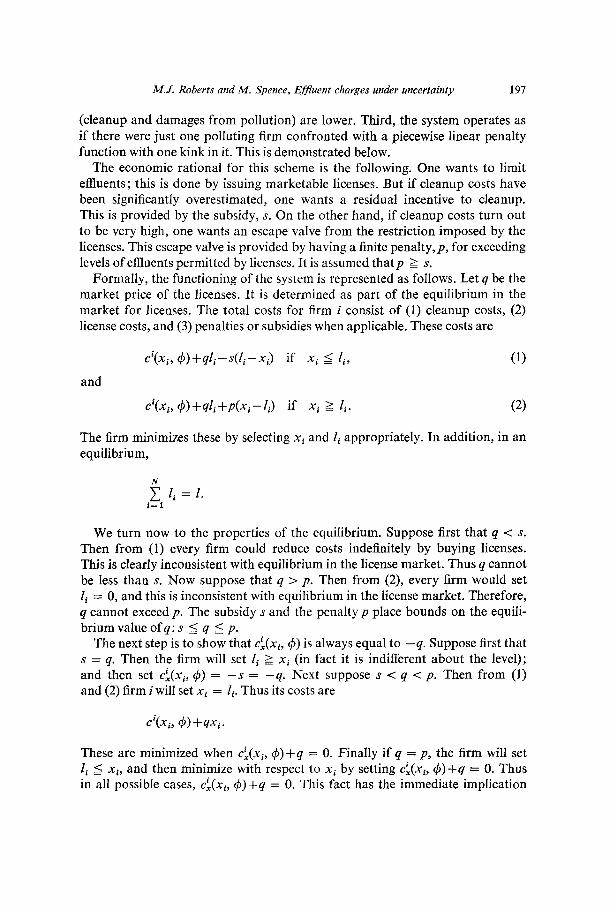
(cleanup and damages from pollution) are lower. Third, the system operates as if there were just one polluting firm confronted with a piecewise linear penalty function with one kink in it. This is demonstrated below.

The economic rational for this scheme is the following. One wants to limit effluents; this is done by issuing marketable licenses. But if cleanup costs have been significantly overestimated, one wants a residual incentive to cleanup. This is provided by the subsidy, s. On the other hand, if cleanup costs turn out to be very high, one wants an escape valve from the restriction imposed by the licenses. This escape valve is provided by having a finite penalty, p, for exceeding levels of effluents permitted by licenses. It is assumed thatp L s.

Formally, the functioning of the system is represented as follows. Let q be the market price of the licenses. It is determined as part of the equilibrium in the market for licenses. The total costs for firm i consist of (1) cleanup costs, (2) license costs, and (3) penalties or subsidies when applicable. These costs are

Ci(Xi, +)+qZi-S(Zi-Xi) if Xi 5 Ii, (1)

and

Ci(Xi, +)+qZi+p(Xi-Ii) if Xi 2 Zi. (2)

The firm minimizes these by selecting xi and Ii appropriately. In addition, in an equilibrium,

We turn now to the properties of the equilibrium. Suppose first that q < s.

Then from (1) every firm could reduce costs indefinitely by buying licenses. This is clearly inconsistent with equilibrium in the license market. Thus q cannot be less than s. Now suppose that q > p. Then from (2), every firm would set Zi = 0, and this is inconsistent with equilibrium in the license market. Therefore, q cannot exceed p. The subsidy s and the penalty p place bounds on the equilibrium value of q: s S q 5 p.

The next step is to show that &(xi, 4) is always equal to -4. Suppose first that s = q. Then the firm will set Ii 2 Xi (in fact it is indifferent about the level); and then set c~(-)Ci, 4) = --s = -4. Next suppose s < q < p. Then from (1) and (2) firm i will set xi = Zi. Thus its costs are

These are minimized when &xi, q%)+q = 0. Finally if q = p, the firm will set Zi 5 Xi, and then minimize with respect to xi by setting Cl(Xi, 4)+q = 0. Thus in all possible cases, &xi, #~)+q = 0. This fact has the immediate implication


that c~(Xi, 4) = &xi, 4) for all i and j, so that cleanup is efficiently distributed among polluters5 In addition 4 is bounded by the effluent subsidy s and the penaltyp.

Since marginal cleanup costs are minimized, the condition

c,(x, $I+4 = 0 (3)

is always satisfied. The remaining question is what determines the levels of q and x? Ifs < q c p,

then xi = Ii for all i, and hence x = 1. Condition (3) will be satisfied if

s < -M, 4) <P. (4)

Inequality (4) will hold for some intermediate range of costs of cleanup. If cleanup costs are very high, then q will be driven up to the level of the penalty p.

At that point, effluents will exceed licenses: x > 1. The equilibrium condition is

&, 4)+p = 0.

Finally if costs are low, so that c,(Z, r$) + s < 0, then x < Z and q = s. The level of effluents actually achieved will be given by

c,(x, 4)+s = 0.

In summary: (1) if c,(Z, 4) +s > 0, then c,(x, 4) +s = 0 and q = s; (2) if s < -c,(Z, 4) < p, then x = Z and q = - c,(Z, 4); and (3) if c,(Z, 4) +p < 0, then c,(x, 4) +p = 0 and q = p.

The interesting feature of the mixed effluent-license is that it produces levels of the effluents, conditional on costs, that reproduce exactly the effluents that would occur if (1) the polluting firms were merged (and made cleanup decisions centrally) and (2) they faced a piecewise linear penalty function of the form,

P(x) = sx+p Max (x-Z, 0).

If the firms collectively were to minimize the sum of penalties and cleanup costs, P(x)+c(x, g5), they would act as follows: if s < - c,(Z, 4) < p, they would set x = I; if -c,(Z, 4) < s, they would set c,(x, 4)+s = 0; and if -c,(Z, 4) > p, they would set c,(x, $)+p = 0. But this is exactly what the decentralized system does.

The pure efficient fee and pure license systems are special cases of the mixed system. The pure effluent fee is obtained by setting s = p, at which point the

5Note that c,(x, 4) = c’,(x~, d), for all i, when x is distributed among polluters in a cost minimizing manner.


level of 1 becomes irrelevant. The implicit penalty function is then linear. If s = 0 and p = + co, then we have a pure license system. It is not therefore surprising that the more flexible mixed system can achieve lower expected total costs.

The mixed system implicitly approximates the expected damage function by a piecewise linear penalty (see fig. 1). The same point can be seen in the context

D,c,P

Fig. 1

Fig. 2

of the marginal damages (see fig. 2). The mixed effluent-license system approximates the marginal damage function with a step function.

It is worth noting that the implicit penalty function P(x), does not correspond exactly to the payments by firms for licenses, plus or minus penalties and subsidies. The actual payments depend upon the parameter 4 that determines costs, and not just upon x, the final level of effluents. But if we plot ex post payments as a function of effluents, the result is as in fig. 3.


X

4. The regulatory authority’s optimizing problem

Fig. 3

The decision variables for the regulators are s, p, and 1. The objective is to minimize expected total costs, consisting of damages from pollution and cleanup costs. For given levels of S, p and 1, there will be two critical levels of the cost determining parameter C#J. The first, c$~, is the level of cost such that

c,(E, 41) = s = 0. (7)

Here the marginal cleanup costs are just equal to the effluent subsidy when x = 1. The second value, 4, > 41, is defined by

Here costs are almost high enough to cause the system to have effluents exceed licenses.

Let [0, b] be the support of the distribution f(4). We define x,(4, s) and

~~(42 P) by

and

c,(x,(A s), 4)+s = 0,

c,(x,(4, P), 4) +P = 0.

Expected total costs are


These expected total costs are minimized when the partial derivatives, T,, Tp

and T,, are zero, or when the following conditional expectations hold :

(9)

With perfect information about costs, the authority would set

Fig. 4

for all 4. Let the optimal schedule of effluents, defined by (12), be x*(4). Let a(4) be the effluent levels achieved with the optimal mixed system described above. The relationship between x*(4) and a(4) is depicted in fig. 4. The schedule a(4) crosses x*(4) three times, once in each interval.

The optimizing conditions, (9) through (1 l), are simply conditions for optimal pure effluent fees or licenses on each of the three intervals. For example, eq. (9) is the condition for s to be the optimal pure effluent fee assuming costs vary only on the interval [0, &I. A pure effluent fee schedule crosses the optimal schedule once. Hence, the mixed schedule crosses x*(4) once in each of three intervals. Notice that pure effluent fees induce excessive cleanup when costs are low and too little cleanup when costs are high. This occurs because at low levels of pollution the effluent fee exceeds marginal damages, and conversely. The pure


license scheme has the opposite property. It is insensitive to variations in cleanup costs.

The superiority of the mixed scheme is simply a result of its ability to better approximate the optimal relationship between pollution levels and damages. The exception occurs when the damage function is linear. In that case, 4i = 0, 4Z = b andp = s. The pure eflluent fee system is optimal.

5. Expected gains from using a mixed system

It is not possible in a short paper to comment extensively on the quantitative benefits of the mixed scheme. However, one can isolate the circumstances under which it is likely to yield significant gains. There are two conditions which make the mixed schemed attractive. First, the marginal damages must vary consider- ably with total effluents. Otherwise the pure effluent fee performs quite well. Second, there must be significant uncertainty about the cleanup costs. Otherwise, the pure license scheme performs well. It is perhaps worth noting that when

Table 1

Control scheme Expected total costs

Percentage above the optimum

Optimum (also mixed system) 12.416 0 Pure effluent fee 20.6 66 Pure licenses 18.25 46

marginal cleanup costs do not vary greatly with quantity, an effluent fee system performs poorly even with small amounts of uncertainty. The reason is that actual levels of cleanup may vary wildly with small shifts in the cost function.

The following numerical example illustrates the potential benefits of the mixed system. It assumes there is a threshold level of pollution, 1, below which marginal damages are one, and above which they are six. Costs are assumed to have the form (4/2)(X-~)~, where 4 takes on the values 0.12 and 2.0 with probabilities of one half. A mixed system yields the optimum for this kind of damage function. Table 1 summarizes the results for the various control schemes.

6. Conclusions

When the regulatory authority is uncertain about pollution control costs, the usefulness of monetary incentives to decentralize pollution control decisions is limited by our inability to pick the correct price. That price should be equal to marginal damages and thus depends upon the level of pollution. But it is not known exactly what pollution will be as a function of price because control costs


are known only imperfectly. With a nonlinear damage function, and uncertain irreversible costs, we would like to find some way of confronting each firm with incentives to cleanup that in fact depend upon marginal damages, and hence on total waste output. The combination of the license scheme with subsidies and penalties permits one simultaneously to ensure that all firms face the same marginal costs, but to have that cost vary (within limits) depending on what the aggregate costs of cleanup actually turn out to be. The level of pollution also varies with the aggregate cleanup costs.

The authority has three parameters to manipulate: the subsidy, the penalty and the stock of licenses. The authority knows that pollution will equal the stock of licenses provided the market price turns out to be between the subsidy and the penalty. The subsidy provides a residual incentive for firms to clean up even more when costs are low. The finite penalty provides an escape valve in case costs are very high. The aggregate damage function is approximated by a piecewise linear penalty function. But once the equilibrium in license prices is estab- lished, each firm effectively faces a linear penalty function whose slope is the price of the license. As a result, marginal cleanup costs are equalized and total cleanup costs are minimized.

How useful is this formulation in the real world? First, we do not believe that limiting our attention to regions of increasing marginal damages is a major practical limitation. There are real cases in which marginal damages may decline - adding more waste to a river which is already an open sewer may have few environmental costs. But in general, even damage functions which exhibit such regions also often appear to be characterized by other regions in which marginal costs are increasing. For example, as the organic material in a river increases, and dissolved oxygen levels decline, we appear to move successively through several thresholds as we lose additional species and human uses. And, intuition suggests that output controls are more likely to be favorable in a region of increasing, rather than decreasing, marginal damages.

In practice, the scheme amounts to setting an ambient target (similar to the ambient standards widely used today) and working back to the magnitude of the discharges allowed by that constraint. Then the regulatory authority has to develop some notion about marginal damages in the regions above and below that point in order to set the subsidy and the penalty fee. Even if the regulatory authority does not quantify its uncertainty and compute an optimal schedule, the rough and ready approach should lead to a reasonable set of policies. After- all, in a second-best world with imperfectly maximizing waste sources, the formal optimality of a policy scheme is not necessarily proof of what its actual impact will be.

Like any decentralized approach to pollution control, our scheme has certain serious limitations. It will not provide for efforts to act directly on the environment as opposed to on a waste source. Nor does it ensure that all economies of scale in treatment will be exhausted unless waste sources agree to appropriate

204 M.J. Roberts and M. Spence, Efjuent charges under uncertainty

joint ventures among themselves. We have also not discussed what should be done in the face of natural variations in climate which make it uncertain what damages will in fact result from any waste discharge.‘j All this suggests that a good deal of detailed work would be required to develop a viable set of policies and institutions for any specific circumstances. For example, could we vary policy seasonally or with actual natural conditions?

In theory, we would want a separate system of licenses to control each polluting substance we are concerned with at each geographic point of interest. Since administrative costs will rise with the complexity of the entire scheme, at some point we will need to make a (perhaps crude) compromise between the costs and benefits of additional elaboration and fine-tuning of the system. Note too that we have to construct our markets such that each has enough participants to ensure relatively competitive functioning. Nevertheless, even viewed as a practical measure designed to move us into a better, if not the best, position, we believe the mixed scheme we have proposed has significant merit. Perhaps the next important step is to consider how to set the penalty function in the presence of risk-aversion relative to damages.

Appendix: A generalized decentralization proposition

In the body of the paper, it was argued that expected total costs could be reduced by the use of both licenses and effluent fees, while maintaining the property of efficiently distributing cleanup among polluters. It was pointed out that the system operated as if the firms made a centralized decision against a penalty function with two facets and one kink. We want to argue now that if one is prepared to introduce more than one kind of license, the penalty function can be made to approximate any convex damage function arbitrarily closely. More precisely, by the use of multiple licenses, the system can be made to efficiently distribute costs and implicitly respond to a penalty function with as many kinks as there are types of licenses.

Let 1’ be the number of licenses of typej. Assume that 1’ 5 I1 5 I2 5 . . . 5 1” and that 7’ = 0. Let so, sr, . . ., s,+ 1, be an increasing sequence of numbers with so = 0. Define a penalty function P(X), in the following way:

p(x) = jjIo Csj+l - Sj) Max (X-I’, 0). 64.1)

The function P(X) is depicted in fig. 5. It is piecewise linear with kinks at 7l, . . ., 1”. The slopes of the facets are sl, . . ., s,,+~, respectively.

The question then, is whether a system of licenses and effluent subsidies and penalties can induce the firms to act collectively as if the penalty function P(x)

6For a discussion of some of those issues, see Roberts (1975).


P(x)

i”= 0 i2 P3 X

Fig. 5

had been imposed. Let qj (j = 1, . . ., n) be the market price of the jth type of license. Let xi be the ith firm’s effluents, let 1: be the holdings of thejth type of license by the ith firm, and let ci(xi) be the cleanup cost function for the ith firm. Having identified the ith firm’s variables, we shall suppress the subscript i in what follows. It should be remembered that the following formulae apply to single firms.

The required technique is to confront each firm with the following total cost function :

64.2)

The last term looks very much like the earlier penalty function. The first term represents cleanup costs. The second term is special. The cost function can be interpreted as follows. The firm pays for cleanup. It also pays for the licenses it purchases, but it receives a rebate of sj per license of typej that it holds. Then, having selected the licenses, the firm pays a penalty given by the piecewise linear function,

-sJ Max (x-l’, 0).

The locations of the kinks in this function are determined by the firm, through its license purchases. It is the second term in (A.2) that is crucial, for as we shall see, it has the effect of placing bounds on the license prices, qj*

It remains to show that firms, in maximizing (A.2), efficiently distribute costs and act as if they were one firm facing the penalty function (A. 1).

The first step to show that

sj S qj S sj+l (A-3)


for all j. Suppose first that qj < sj. Then expand Zj so that Zj > x. It follows that the term in (A.2) involving Zj is

By allowing Zj to increase without limit, costs are reduced indefinitely. But that is inconsistent with equilibrium. Now suppose qj > s~+~. Reduce 1’ so that Zj < x and the term involving I’ becomes

(qj-sj)zj-(sj+l -sj)zj = (qj-sj+l)zj.

Hence costs are minimized when Zj = 0. If all firms do this, there cannot be an equilibrium in the market forj-type licenses. Therefore

$j i qj 5 sj+l,

for allj = 1, . . ., n. The next step is to show that if qj < Sj+l, then qj+l = Sj+l. Suppose that

qj < Sj+l. We show that Zj 5 x. Suppose to the contrary that Zj > x. Then the part of costs involving Zj is, from (A.2),

Hence Zj should be contracted. Therefore if qj < sj+i, then Zj 2 x, and Zj+’ > Zj 2 x, so that x is less than Zj+‘. But if Zj+’ > X, then qj+l must equal Sj+l. Forifqj+l > s~+~, then the part of costs involving Zj+’ is

(4j+l-sj+l>zj+19

and Zj+’ would be reduced. Hence if Zj+r > x, then qj+1 = s~+~. This proves the assertionthatifqj < ~~+i,thenq~+~ = s~+~.

These arguments tell us a considerable amount about the equilibrium. Only one license price qj can be in the interior of [sj, s~+~]. The remainder are on the boundaries - upper or lower depending upon whether the corresponding license has a lower or higher index than j, respectively.

We now take a typical interval [sj, Sj+l] and assume qj is the interior of [Sj, Sj+l]. From the preceding argument, we know that Zj = x, that qk = Sk+1 for k < j, and that qk = sk for k > j. Thus the costs for the firm are, from (A.2),

j-l

~(~)+k~o(sk+l-sk~zk+k~~+~k+l-sk)zk

j-l

+k~~(Sk+~-sk)(x-~k)+(~j-~j)x+(~j+l-sj)(o)

= c(x)+qjx.


Similarly, if qj = sj, or qj = s~+~, and if qk = s~+~ for k < j and qk = sk for k > j, then (A.2) implies that the firm’s costs (with licenses optimized out) are

C(X) + qjX *

In an equilibrium, the costs for every firm will be

dx> + 9jx,

for some j and some equilibrium value qj. Thus when firms minimize, with respect to x, they set

C’(X)+qj = 0. (A-4)

In particular, marginal cleanup costs, c’(x), are the same for every firm. There- fore cleanup costs are efficiently distributed in an equilibrium. Let C(X) be the aggregate cost function, where x is now the sum of the effluents from all firms. In an equilibrium, (A.4) implies that

C’(X)+qj = 0.

Moreover, if Sj < qj < Sj+l, then x = I’, where lj is the fixed total number of j-type licenses. If qj = sj, then ij-l < x 5 I’, and if qj = s~+~, then ij < x 2 /j+l. The equilibrium level of x is therefore determined by the level of costs. If

Sj < -C'(i') < Sj+l, (A.5)

then x = 1’ in an equilibrium. If - C’(ij) < sj and - C’(lj-I) > Sj, then C’(x) = sj in the equilibrium. 7

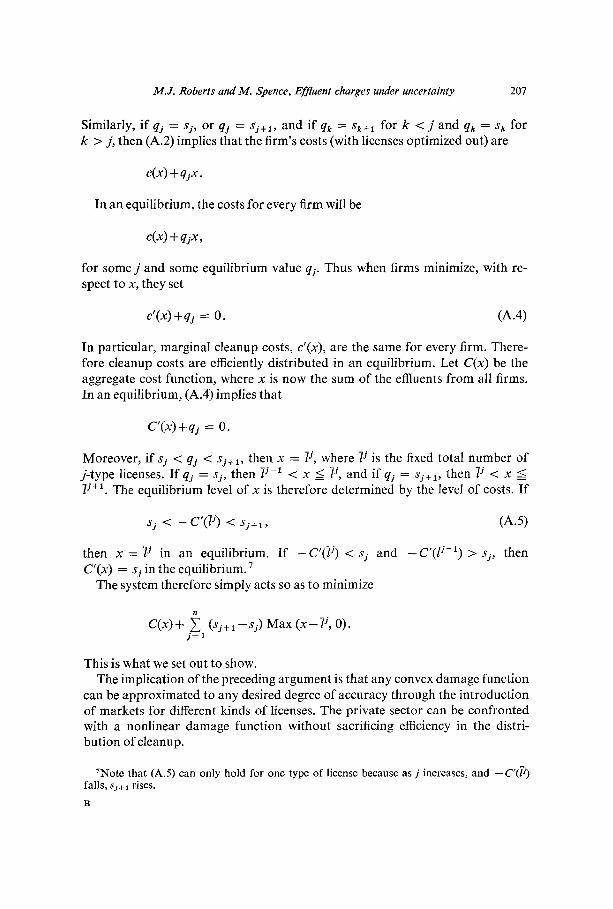
The system therefore simply acts so as to minimize

C(X)+ i (sj+l -sj) Max (x-ii, 0). j=l

This is what we set out to show. The implication of the preceding argument is that any convex damage function

can be approximated to any desired degree of accuracy through the introduction of markets for different kinds of licenses. The private sector can be confronted with a nonlinear damage function without sacrificing efficiency in the distribution of cleanup.

7Note that (A.5) can only hold for one type of license because as j increases, and -C@) falls, s~+~ rises.

B


As a practical matter, in the pollution context, the cost of the additional license markets may not be justified by the reduction in expected total cost. But it is perhaps a matter of some intellectual interest, both here and in other decentralization problems, that a carefully designed set of markets for options to buy or sell commodities at various prices can solve the problem of reconciling the competing demands of efficiency and decentralization. This subject is pro- bably worthy of further investigation.

References

Jacoby, H., G. Schaumberg and F. Gramlech, 1972, Marketable pollution rights (M.I.T., Cambridge, MA) unpublished.

Kneese, A.V. and B. Bower, 1968, Managing water quality (Resources for the Future, Johns Hopkins Press, Baltimore).

Montgomery, W.C., 1972, Markets in licenses and efficient pollution control programs, Journal of Economic Theory 5, no. 3,395-418.

Roberts, M.J., 1975, Environmental protection: The complexities of real policy choice, in: Fox and Swainson, eds., Water quality management: The design of institutional arrange- ments (University of British Columbia Press, Vancouver).

Roberts Spence JPubE 1976

Documents

Transcript of Roberts Spence JPubE 1976