Robert Collins CSE486 - Penn State College of …rtc12/CSE486/lecture11.pdf · CSE486 Robert...
37
CSE486 Robert Collins Lecture 11: LoG and DoG Filters
Transcript of Robert Collins CSE486 - Penn State College of …rtc12/CSE486/lecture11.pdf · CSE486 Robert...
CSE486Robert Collins
Lecture 11:LoG and DoG Filters
CSE486Robert Collins
Today’s Topics
Laplacian of Gaussian (LoG) Filter - useful for finding edges - also useful for finding blobs!
approximation using Difference of Gaussian (DoG)
CSE486Robert Collins
Recall: First Derivative Filters
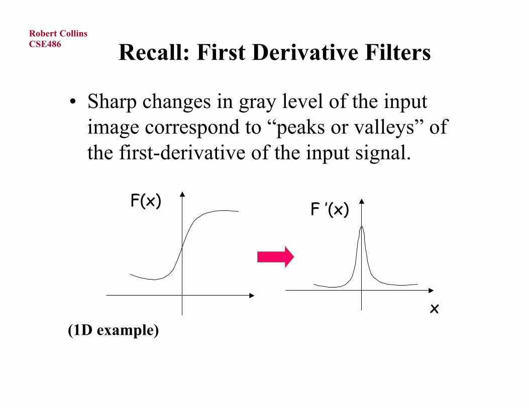
• Sharp changes in gray level of the inputimage correspond to “peaks or valleys” ofthe first-derivative of the input signal.
F(x)F(x) F F ’’(x)(x)
xx
O.Camps, PSU
(1D example)
CSE486Robert Collins
Second-Derivative Filters
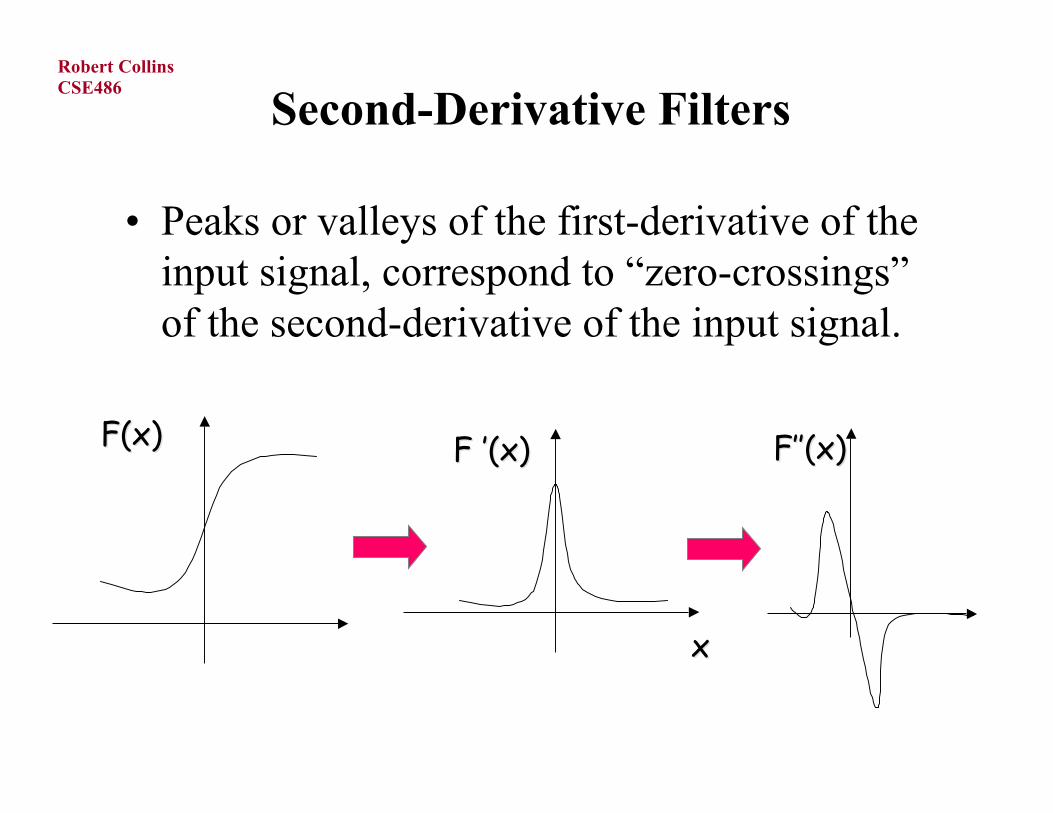
• Peaks or valleys of the first-derivative of theinput signal, correspond to “zero-crossings”of the second-derivative of the input signal.
F(x)F(x) F F ’’(x)(x)
xx
FF’’’’(x)(x)
O.Camps, PSU
CSE486Robert Collins
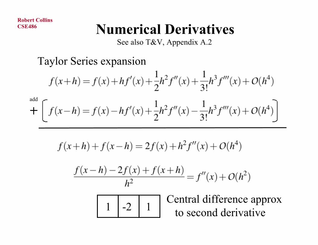
Numerical DerivativesSee also T&V, Appendix A.2
Taylor Series expansion
1 -2 1Central difference approx to second derivative
add
CSE486Robert Collins
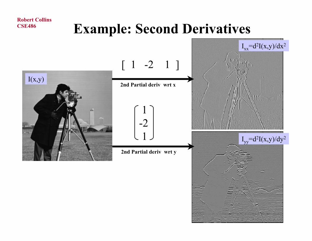
Example: Second Derivatives
I(x,y)
Ixx=d2I(x,y)/dx2
Iyy=d2I(x,y)/dy2
2nd Partial deriv wrt x
2nd Partial deriv wrt y
[ 1 -2 1 ]
1 -2 1
CSE486Robert Collins
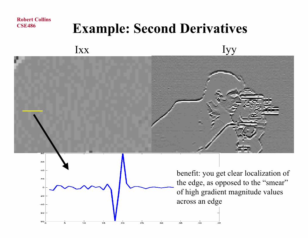
Example: Second Derivatives
Ixx Iyy
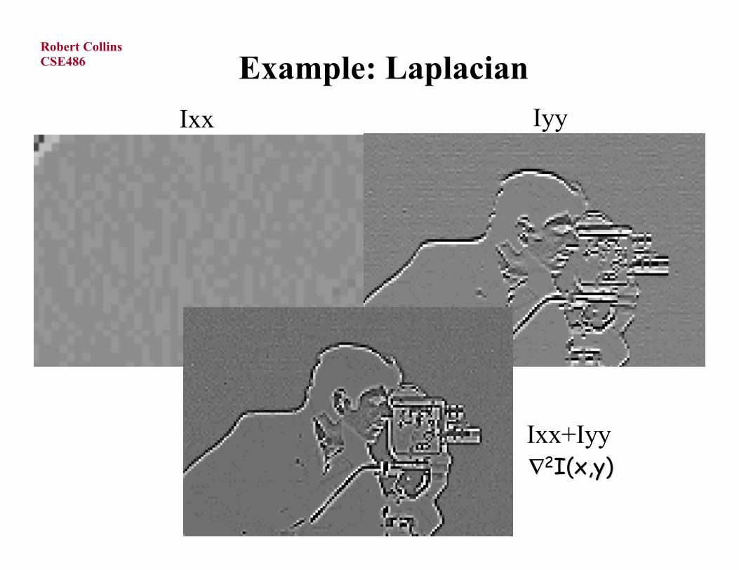
benefit: you get clear localization ofthe edge, as opposed to the “smear”of high gradient magnitude valuesacross an edge
CSE486Robert Collins
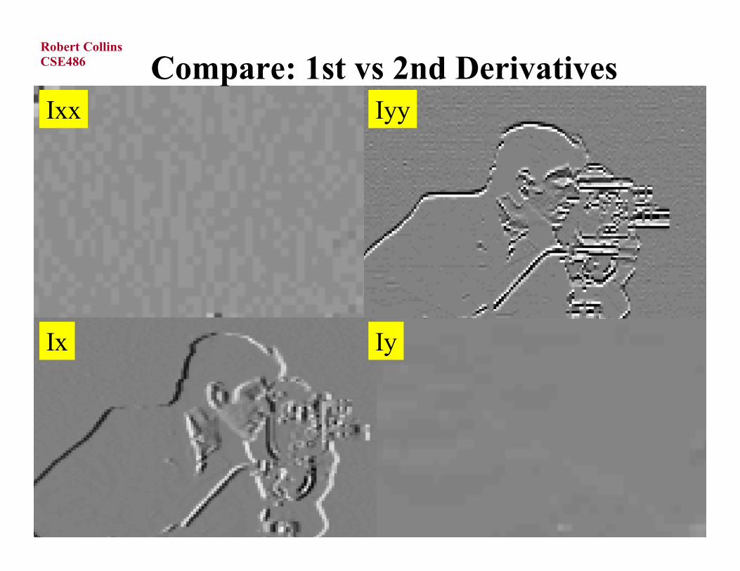
Compare: 1st vs 2nd DerivativesIxx Iyy
Ix Iy
CSE486Robert Collins
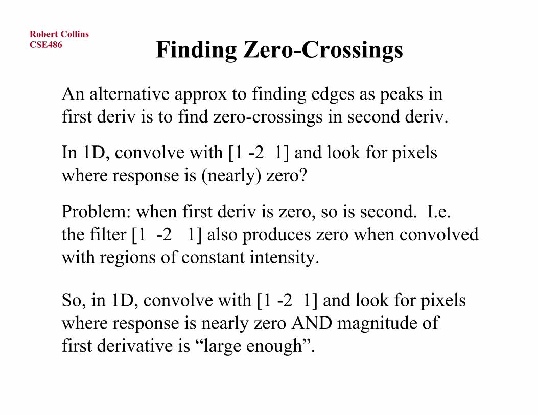
Finding Zero-Crossings
An alternative approx to finding edges as peaks infirst deriv is to find zero-crossings in second deriv.
In 1D, convolve with [1 -2 1] and look for pixels where response is (nearly) zero?
Problem: when first deriv is zero, so is second. I.e.the filter [1 -2 1] also produces zero when convolvedwith regions of constant intensity.
So, in 1D, convolve with [1 -2 1] and look for pixelswhere response is nearly zero AND magnitude offirst derivative is “large enough”.
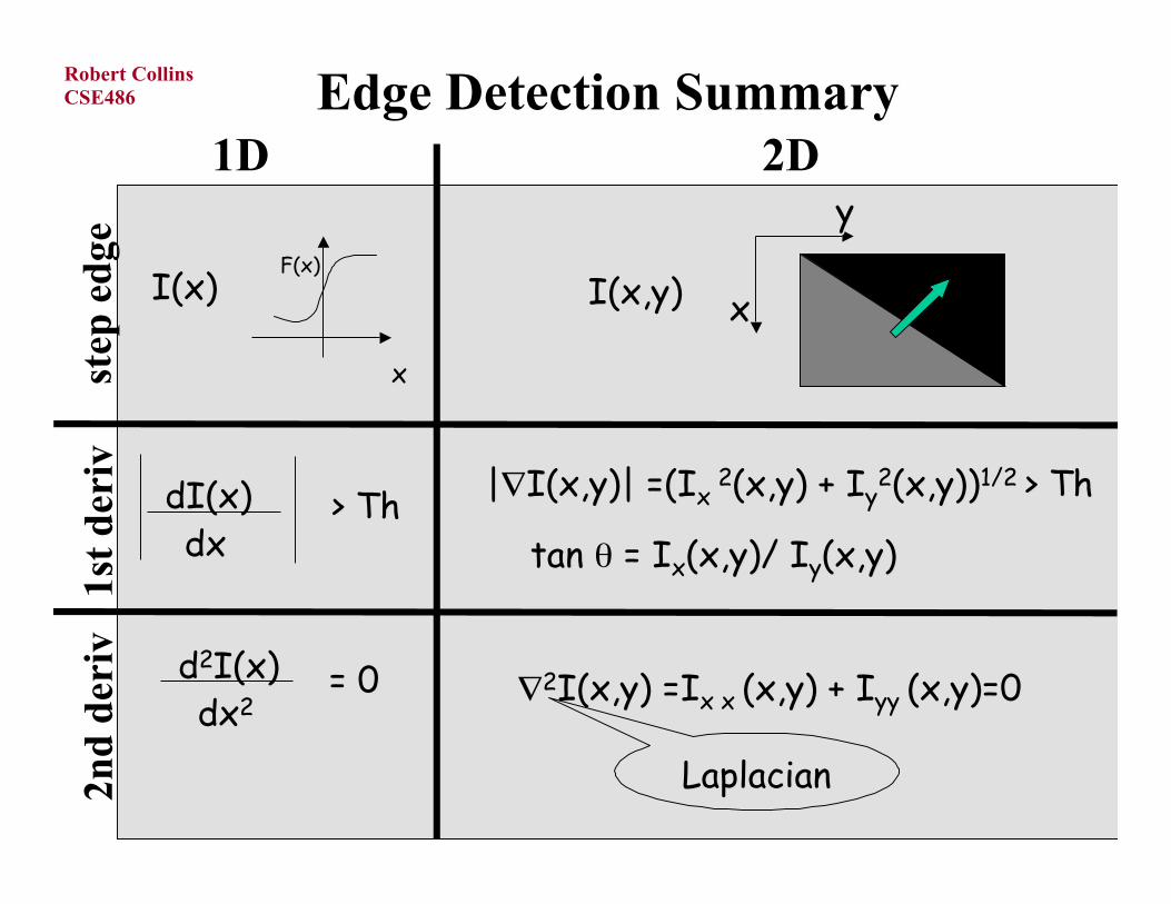
CSE486Robert Collins Edge Detection Summary
I(x)I(x) I(x,y)I(x,y)
dd22I(x)I(x)dxdx22
= 0= 0
xx
yy
||∇∇I(x,y)| =(II(x,y)| =(Ix x 22(x,y) + I(x,y) + Iyy
22(x,y))(x,y))1/2 1/2 > > ThTh
tan tan θθ = I = Ixx(x,y)/ (x,y)/ IIyy(x,y) (x,y)
F(x)F(x)
xx
dI(x)dI(x)dxdx
> > ThTh
∇∇22I(x,y) =II(x,y) =Ix x x x (x,y) + (x,y) + IIyy yy (x,y)=0(x,y)=0
LaplacianLaplacian
1D 2Dst
ep e
dge
1st
deri
v2n
d de
riv
CSE486Robert Collins
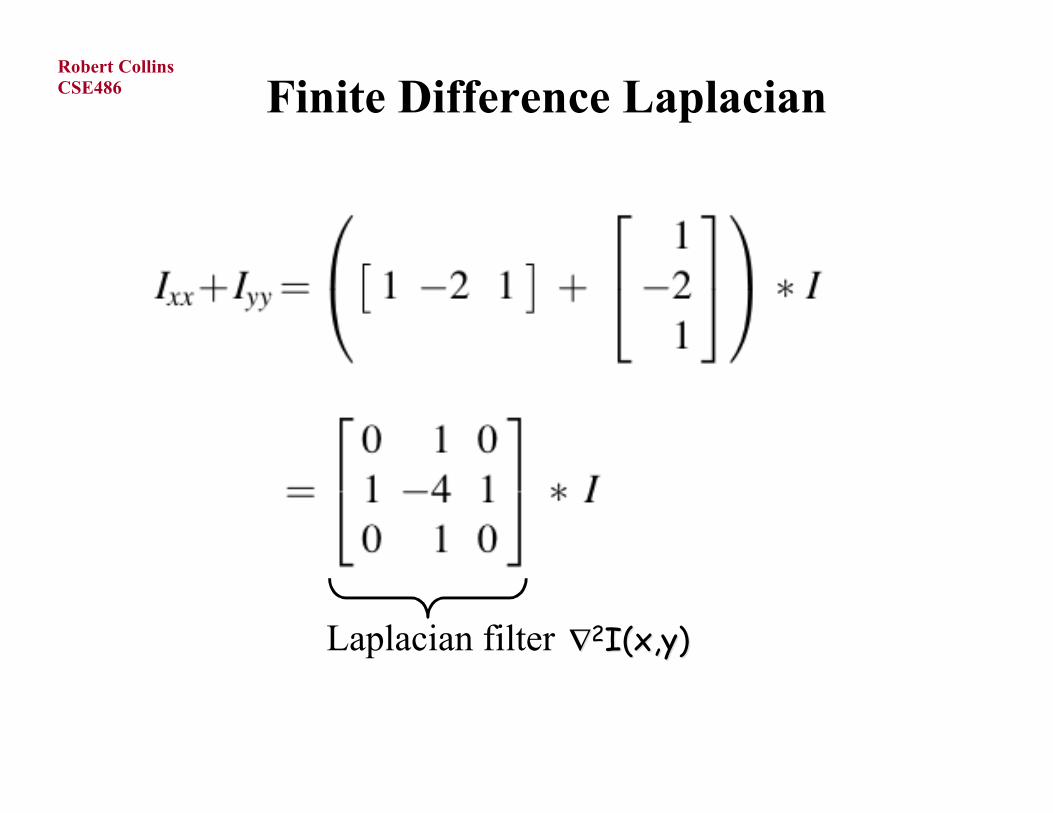
Finite Difference Laplacian
Laplacian filter ∇∇22I(x,y)I(x,y)
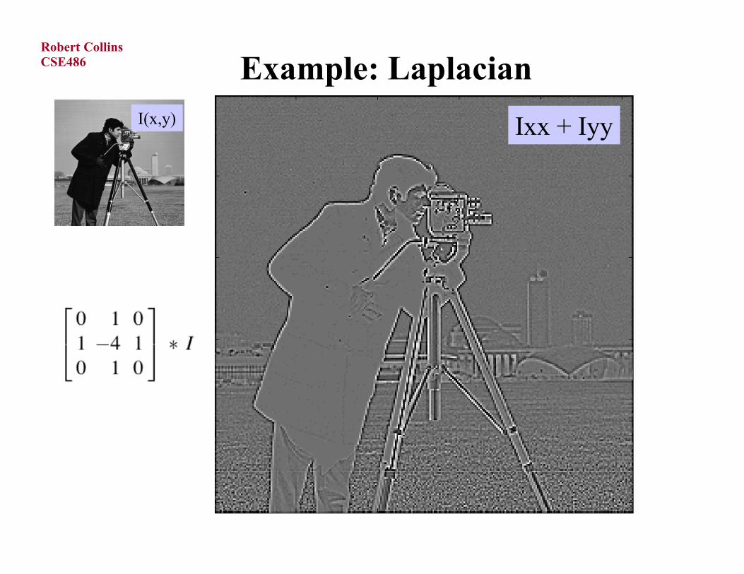
CSE486Robert Collins
Example: LaplacianI(x,y) Ixx + Iyy
CSE486Robert Collins
Example: Laplacian
Ixx Iyy
Ixx+Iyy∇∇22I(x,y)I(x,y)
CSE486Robert Collins
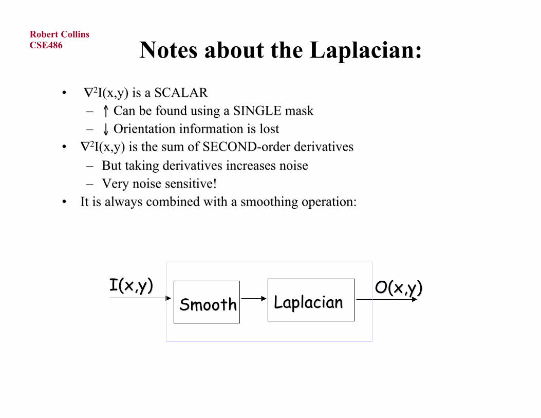
Notes about the Laplacian:
• ∇∇22I(x,y) is a SCALARI(x,y) is a SCALAR–– ↑↑ Can be found using a SINGLE mask Can be found using a SINGLE mask–– ↓↓ Orientation information is lost Orientation information is lost
•• ∇∇22I(x,y) is the sum of SECOND-order derivativesI(x,y) is the sum of SECOND-order derivatives
–– But taking derivatives increases noiseBut taking derivatives increases noise–– Very noise sensitive!Very noise sensitive!
•• It is always combined with a smoothing operation:It is always combined with a smoothing operation:
SmoothSmooth LaplacianLaplacianI(x,y)I(x,y) O(x,y)O(x,y)
O.Camps, PSU
CSE486Robert Collins
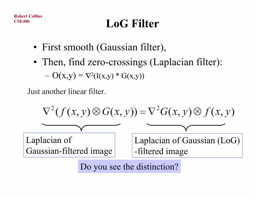
LoG Filter
• First smooth (Gaussian filter),
• Then, find zero-crossings (Laplacian filter):– O(x,y) = ∇∇22((I(x,y) * G(x,y))I(x,y) * G(x,y))
O.Camps, PSU
Laplacian of Gaussian-filtered image
Laplacian of Gaussian (LoG)-filtered image
Do you see the distinction?
CSE486Robert Collins
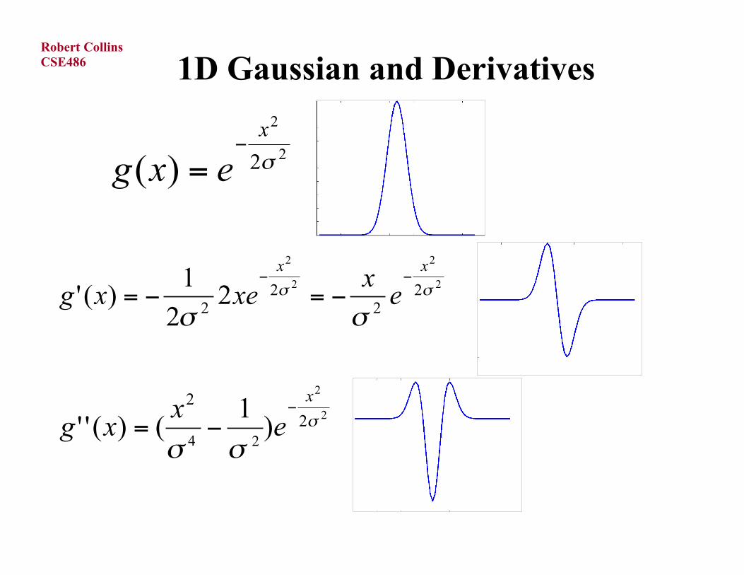
1D Gaussian and Derivatives
2
2
2)( σ
x
exg−
=
2
2
2
2
22
222
2
1)(' σσ
σσ
xx
ex
xexg−−
−=−=
O.Camps, PSU
2
2
23
2
)1
()('' σ
σσ
x
ex
xg−
−=24
CSE486Robert Collins
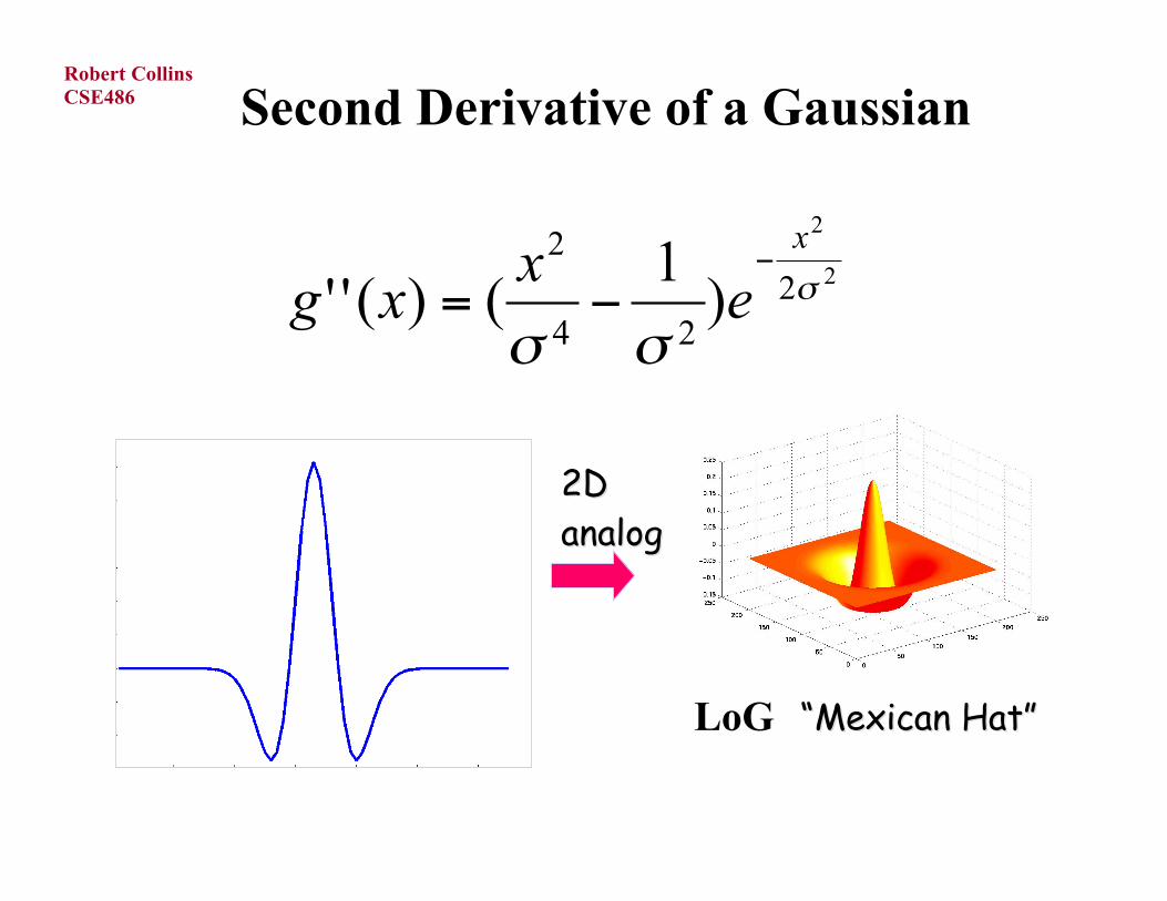
Second Derivative of a Gaussian
2D2Danaloganalog
““Mexican HatMexican Hat””
O.Camps, PSU
LoG
2
2
23
2
)1
()('' σ
σσ
x
ex
xg−
−=4 2
CSE486Robert Collins
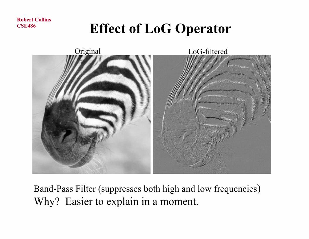
Effect of LoG Operator
LoG-filteredOriginal
Band-Pass Filter (suppresses both high and low frequencies)Why? Easier to explain in a moment.
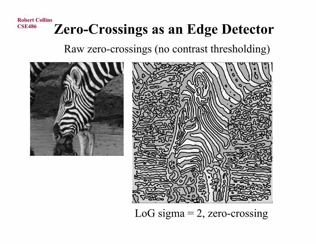
CSE486Robert Collins
Zero-Crossings as an Edge DetectorRaw zero-crossings (no contrast thresholding)
LoG sigma = 2, zero-crossing
CSE486Robert Collins
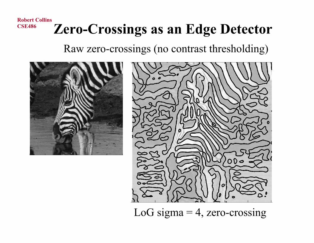
Raw zero-crossings (no contrast thresholding)
LoG sigma = 4, zero-crossing
Zero-Crossings as an Edge Detector

CSE486Robert Collins
Zero-Crossings as an Edge DetectorRaw zero-crossings (no contrast thresholding)
LoG sigma = 8, zero-crossing
CSE486Robert Collins
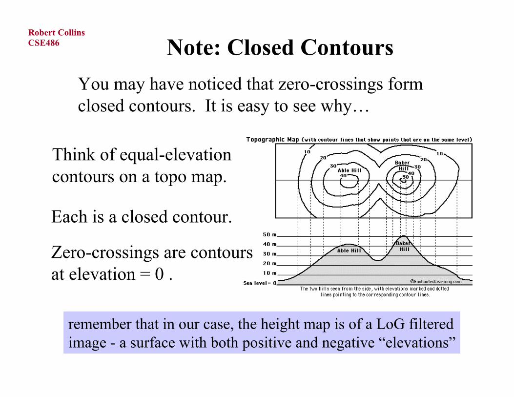
Note: Closed Contours
You may have noticed that zero-crossings formclosed contours. It is easy to see why…
Think of equal-elevationcontours on a topo map.
Each is a closed contour.
Zero-crossings are contoursat elevation = 0 .
remember that in our case, the height map is of a LoG filteredimage - a surface with both positive and negative “elevations”
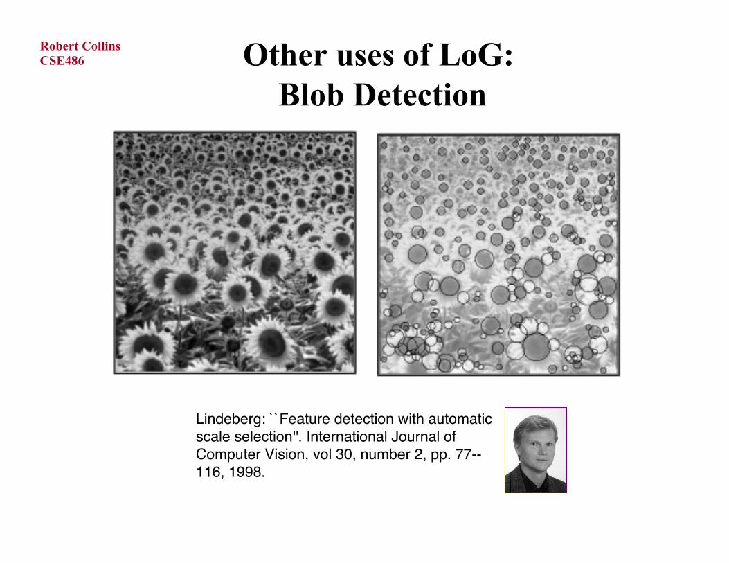
CSE486Robert Collins Other uses of LoG:
Blob Detection
Lindeberg: ``Feature detection with automaticscale selection''. International Journal ofComputer Vision, vol 30, number 2, pp. 77--116, 1998.

CSE486Robert Collins
Pause to Think for a Moment:
How can an edge finder also be used tofind blobs in an image?
CSE486Robert Collins
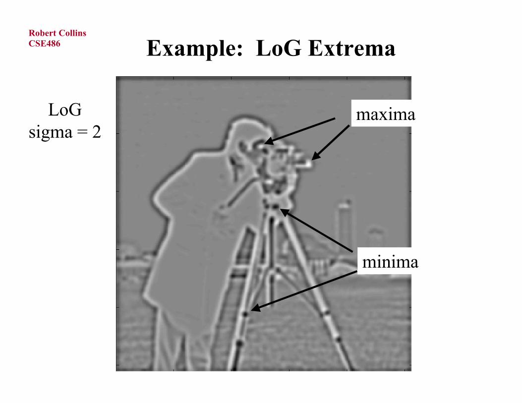
Example: LoG Extrema
LoGsigma = 2
maxima
minima
CSE486Robert Collins
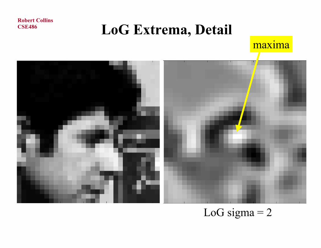
LoG Extrema, Detail
LoG sigma = 2
maxima
CSE486Robert Collins
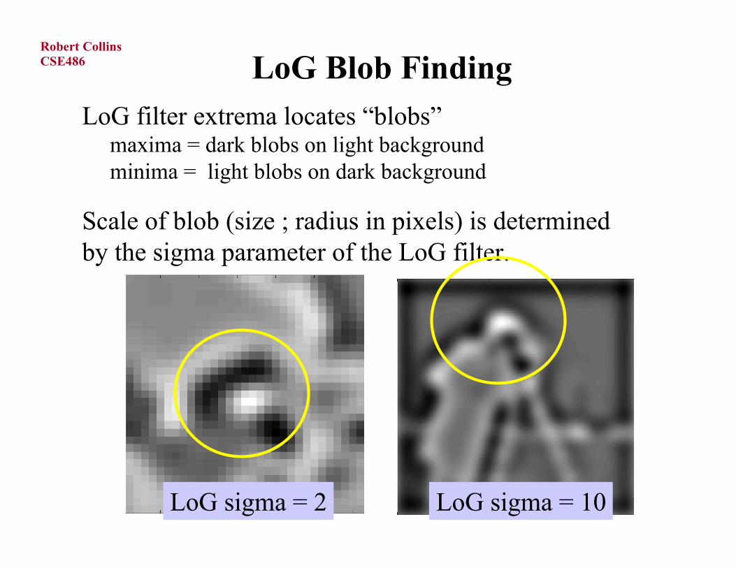
LoG Blob FindingLoG filter extrema locates “blobs” maxima = dark blobs on light background minima = light blobs on dark background
Scale of blob (size ; radius in pixels) is determinedby the sigma parameter of the LoG filter.
LoG sigma = 2 LoG sigma = 10
CSE486Robert Collins
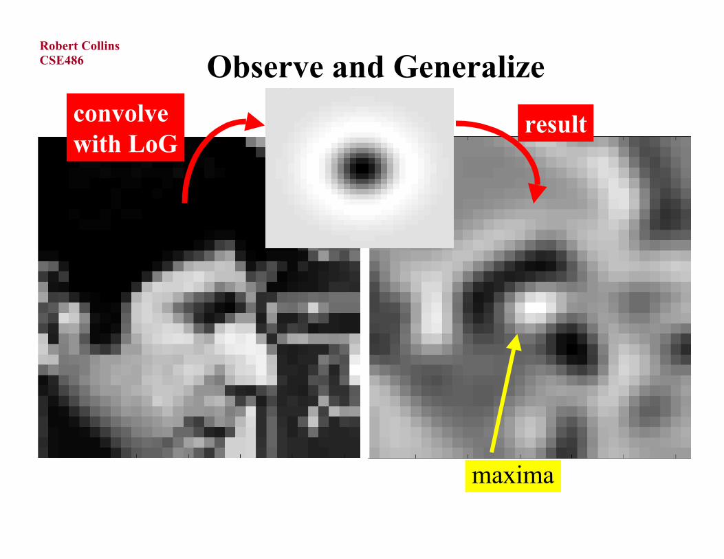
Observe and Generalize
maxima
convolvewith LoG
result
CSE486Robert Collins
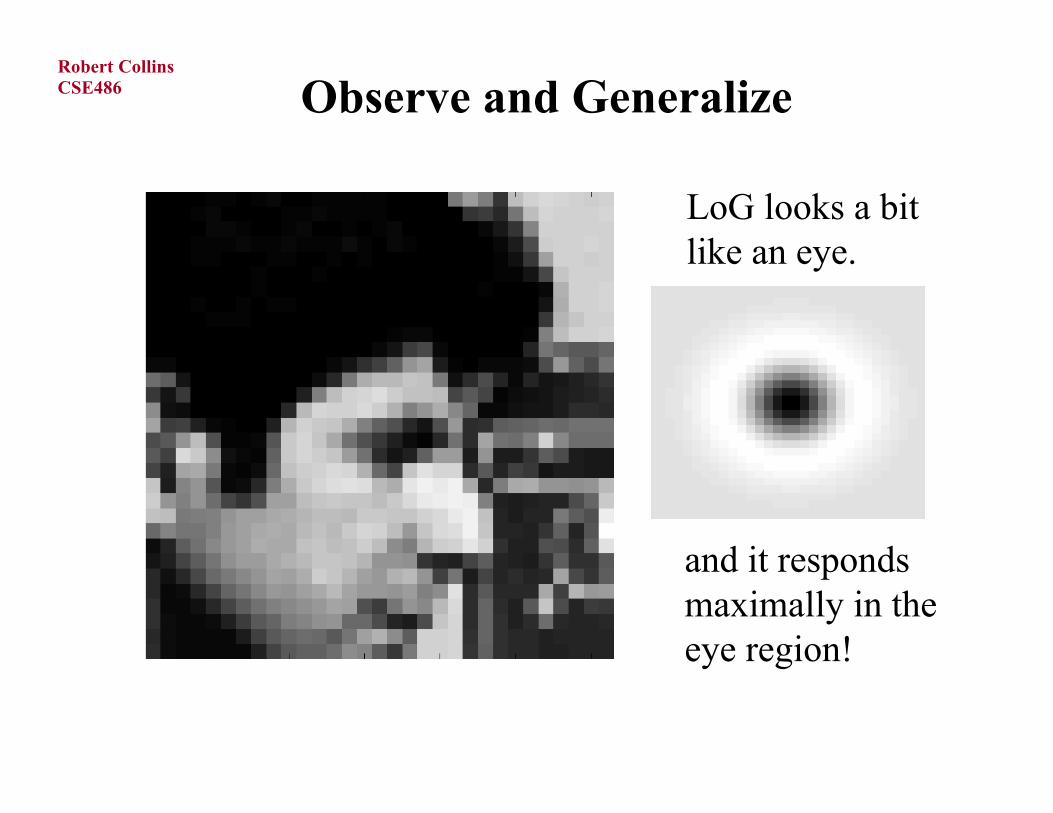
Observe and Generalize
LoG looks a bit like an eye.
and it respondsmaximally in theeye region!
CSE486Robert Collins
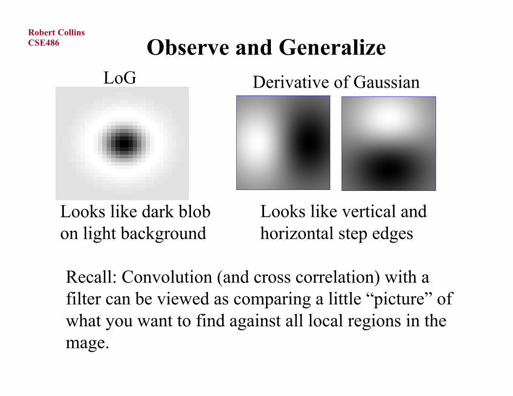
Observe and Generalize
Looks like dark blob on light background
LoG Derivative of Gaussian
Looks like vertical andhorizontal step edges
Recall: Convolution (and cross correlation) with a filter can be viewed as comparing a little “picture” of what you want to find against all local regions in themage.
CSE486Robert Collins
Observe and Generalize
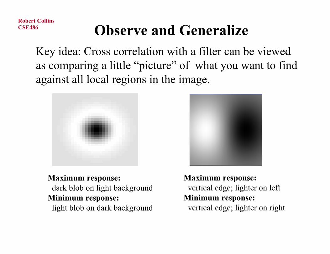
Maximum response: dark blob on light backgroundMinimum response: light blob on dark background
Key idea: Cross correlation with a filter can be viewed as comparing a little “picture” of what you want to find against all local regions in the image.
Maximum response: vertical edge; lighter on leftMinimum response: vertical edge; lighter on right
CSE486Robert Collins Efficient Implementation
Approximating LoG with DoG
M.Hebert, CMU
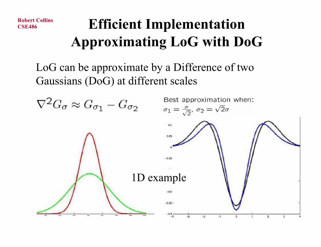
LoG can be approximate by a Difference of two Gaussians (DoG) at different scales
1D example
CSE486Robert Collins
Efficient Implementation
LoG can be approximate by a Difference of two Gaussians (DoG) at different scales.
Separability of and cascadability of Gaussians appliesto the DoG, so we can achieve efficient implementationof the LoG operator.
DoG approx also explains bandpass filtering of LoG(think about it. Hint: Gaussian is a low-pass filter)
CSE486Robert Collins
Back to Blob Detection
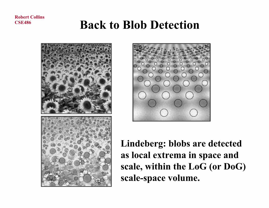
Lindeberg: blobs are detectedas local extrema in space and scale, within the LoG (or DoG)scale-space volume.

CSE486Robert Collins Other uses of LoG:
Blob Detection
Gesture recognition forthe ultimate couch potato
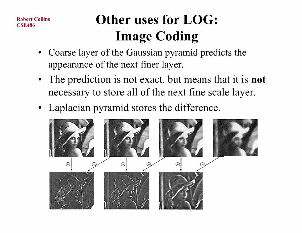
CSE486Robert Collins Other uses for LOG:
Image Coding• Coarse layer of the Gaussian pyramid predicts the
appearance of the next finer layer.
• The prediction is not exact, but means that it is notnecessary to store all of the next fine scale layer.
• Laplacian pyramid stores the difference.
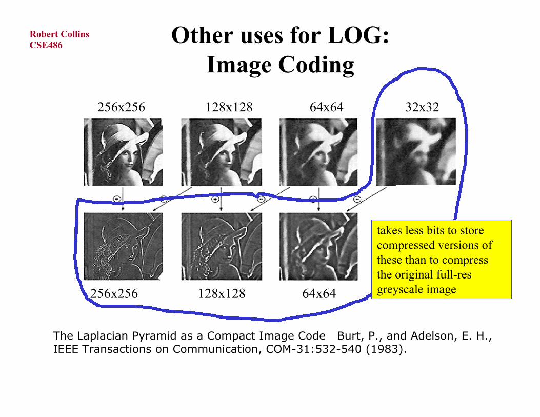
CSE486Robert Collins Other uses for LOG:
Image Coding
256x256 128x128 32x3264x64
256x256 128x128 64x64
The Laplacian Pyramid as a Compact Image Code Burt, P., and Adelson, E. H.,IEEE Transactions on Communication, COM-31:532-540 (1983).
takes less bits to storecompressed versions ofthese than to compressthe original full-resgreyscale image