![Forecasting using - Rob J Hyndman exponential smoothing Forecasting using R Simple exponential smoothing 9 animation by animate[2012/05/24] Simple exponential smoothing Optimization](https://static.fdocuments.in/doc/165x107/5aae58377f8b9a07498bfac5/forecasting-using-rob-j-hyndman-exponential-smoothing-forecasting-using-r-simple.jpg)
Rob J Hyndman Automatic algorithms for time … algorithms for time series forecasting 3 Motivation...
129
Rob J Hyndman Automatic algorithms for time series forecasting
-
Upload
truongminh -
Category
Documents
-
view
225 -
download
0
Transcript of Rob J Hyndman Automatic algorithms for time … algorithms for time series forecasting 3 Motivation...
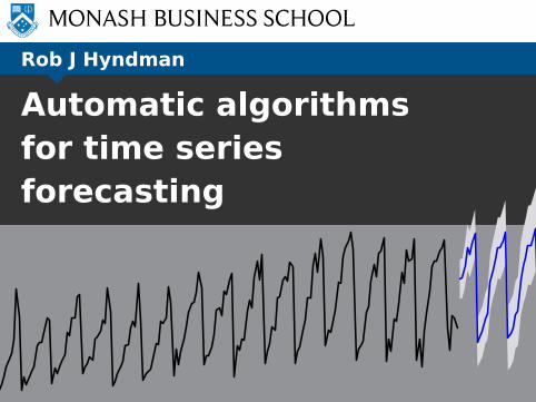
Rob J Hyndman
Automatic algorithmsfor time seriesforecasting
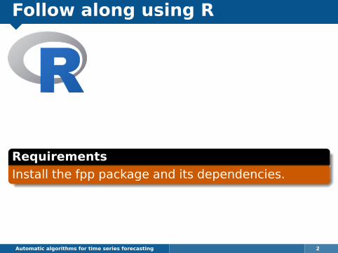
Follow along using R
Requirements
Install the fpp package and its dependencies.
Automatic algorithms for time series forecasting 2
Motivation
1 Common in business to have over 1000products that need forecasting at least monthly.
2 Forecasts are often required by people who areuntrained in time series analysis.
Specifications
Automatic forecasting algorithms must:
å determine an appropriate time series model;
å estimate the parameters;
å compute the forecasts with prediction intervals.
Automatic algorithms for time series forecasting 3
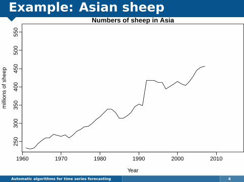
Example: Asian sheep
Automatic algorithms for time series forecasting 4
Numbers of sheep in Asia
Year
mill
ions
of s
heep
1960 1970 1980 1990 2000 2010
250
300
350
400
450
500
550

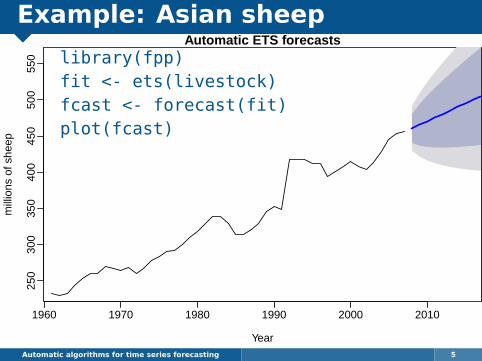
Example: Asian sheep
Automatic algorithms for time series forecasting 4
Automatic ETS forecasts
Year
mill
ions
of s
heep
1960 1970 1980 1990 2000 2010
250
300
350
400
450
500
550
Example: Asian sheep
library(fpp)fit <- ets(livestock)fcast <- forecast(fit)plot(fcast)
Automatic algorithms for time series forecasting 5
Automatic ETS forecasts
Year
mill
ions
of s
heep
1960 1970 1980 1990 2000 2010
250
300
350
400
450
500
550

Example: Cortecosteroid sales
Automatic algorithms for time series forecasting 6
Monthly cortecosteroid drug sales in Australia
Year
Tota
l scr
ipts
(m
illio
ns)
1995 2000 2005 2010
0.4
0.6
0.8
1.0
1.2
1.4
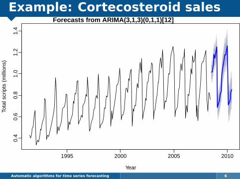
Example: Cortecosteroid sales
Automatic algorithms for time series forecasting 6
Forecasts from ARIMA(3,1,3)(0,1,1)[12]
Year
Tota
l scr
ipts
(m
illio
ns)
1995 2000 2005 2010
0.4
0.6
0.8
1.0
1.2
1.4
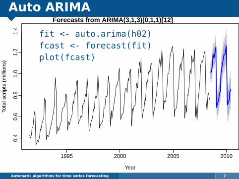
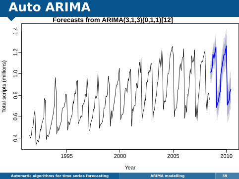
Auto ARIMA
fit <- auto.arima(h02)fcast <- forecast(fit)plot(fcast)
Automatic algorithms for time series forecasting 7
Forecasts from ARIMA(3,1,3)(0,1,1)[12]
Year
Tota
l scr
ipts
(m
illio
ns)
1995 2000 2005 2010
0.4
0.6
0.8
1.0
1.2
1.4
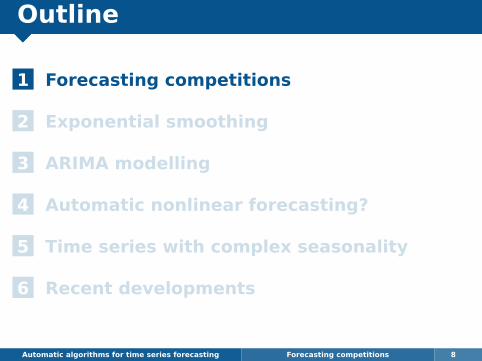
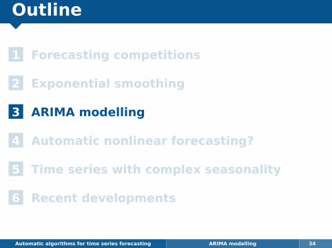
Outline
1 Forecasting competitions
2 Exponential smoothing
3 ARIMA modelling
4 Automatic nonlinear forecasting?
5 Time series with complex seasonality
6 Recent developments
Automatic algorithms for time series forecasting Forecasting competitions 8

Makridakis and Hibon (1979)
Automatic algorithms for time series forecasting Forecasting competitions 9

Makridakis and Hibon (1979)
Automatic algorithms for time series forecasting Forecasting competitions 9
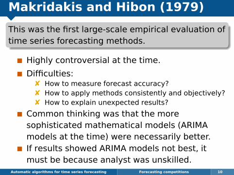
Makridakis and Hibon (1979)
This was the first large-scale empirical evaluation oftime series forecasting methods.
Highly controversial at the time.
Difficulties:8 How to measure forecast accuracy?8 How to apply methods consistently and objectively?8 How to explain unexpected results?
Common thinking was that the moresophisticated mathematical models (ARIMAmodels at the time) were necessarily better.If results showed ARIMA models not best, itmust be because analyst was unskilled.
Automatic algorithms for time series forecasting Forecasting competitions 10
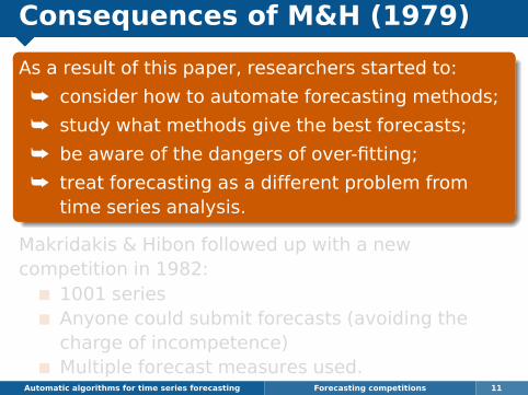
Consequences of M&H (1979)
As a result of this paper, researchers started to:
å consider how to automate forecasting methods;
å study what methods give the best forecasts;
å be aware of the dangers of over-fitting;
å treat forecasting as a different problem fromtime series analysis.
Makridakis & Hibon followed up with a newcompetition in 1982:
1001 seriesAnyone could submit forecasts (avoiding thecharge of incompetence)Multiple forecast measures used.
Automatic algorithms for time series forecasting Forecasting competitions 11
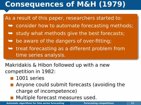

M-competition
Automatic algorithms for time series forecasting Forecasting competitions 12
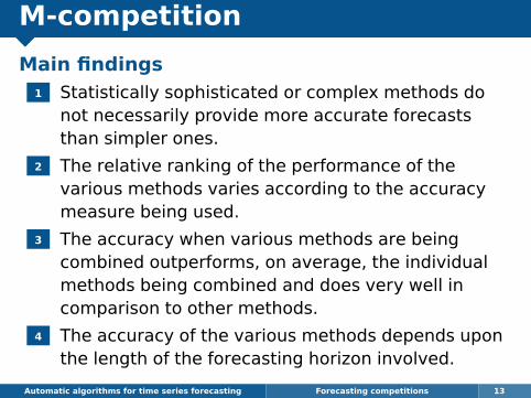
M-competition
Main findings1 Statistically sophisticated or complex methods do
not necessarily provide more accurate forecaststhan simpler ones.
2 The relative ranking of the performance of thevarious methods varies according to the accuracymeasure being used.
3 The accuracy when various methods are beingcombined outperforms, on average, the individualmethods being combined and does very well incomparison to other methods.
4 The accuracy of the various methods depends uponthe length of the forecasting horizon involved.
Automatic algorithms for time series forecasting Forecasting competitions 13

M3 competition
Automatic algorithms for time series forecasting Forecasting competitions 14
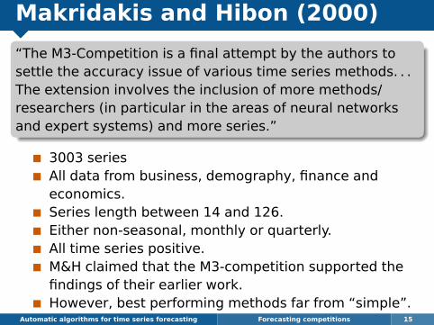
Makridakis and Hibon (2000)
“The M3-Competition is a final attempt by the authors tosettle the accuracy issue of various time series methods. . .The extension involves the inclusion of more methods/researchers (in particular in the areas of neural networksand expert systems) and more series.”
3003 seriesAll data from business, demography, finance andeconomics.Series length between 14 and 126.Either non-seasonal, monthly or quarterly.All time series positive.M&H claimed that the M3-competition supported thefindings of their earlier work.However, best performing methods far from “simple”.
Automatic algorithms for time series forecasting Forecasting competitions 15
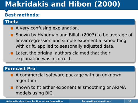
Makridakis and Hibon (2000)Best methods:
Theta
A very confusing explanation.
Shown by Hyndman and Billah (2003) to be average oflinear regression and simple exponential smoothingwith drift, applied to seasonally adjusted data.
Later, the original authors claimed that theirexplanation was incorrect.
Forecast Pro
A commercial software package with an unknownalgorithm.
Known to fit either exponential smoothing or ARIMAmodels using BIC.
Automatic algorithms for time series forecasting Forecasting competitions 16
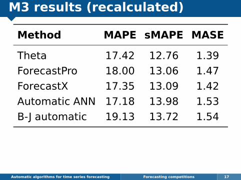
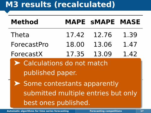
M3 results (recalculated)
Method MAPE sMAPE MASE
Theta 17.42 12.76 1.39
ForecastPro 18.00 13.06 1.47
ForecastX 17.35 13.09 1.42
Automatic ANN 17.18 13.98 1.53
B-J automatic 19.13 13.72 1.54
Automatic algorithms for time series forecasting Forecasting competitions 17
M3 results (recalculated)
Method MAPE sMAPE MASE
Theta 17.42 12.76 1.39
ForecastPro 18.00 13.06 1.47
ForecastX 17.35 13.09 1.42
Automatic ANN 17.18 13.98 1.53
B-J automatic 19.13 13.72 1.54
Automatic algorithms for time series forecasting Forecasting competitions 17
ä Calculations do not match
published paper.
ä Some contestants apparently
submitted multiple entries but only
best ones published.
Outline
1 Forecasting competitions
2 Exponential smoothing
3 ARIMA modelling
4 Automatic nonlinear forecasting?
5 Time series with complex seasonality
6 Recent developments
Automatic algorithms for time series forecasting Exponential smoothing 18
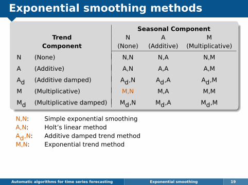
Exponential smoothing methods
Seasonal ComponentTrend N A M
Component (None) (Additive) (Multiplicative)
N (None) N,N N,A N,M
A (Additive) A,N A,A A,M
Ad (Additive damped) Ad,N Ad,A Ad,M
M (Multiplicative) M,N M,A M,M
Md (Multiplicative damped) Md,N Md,A Md,M
Automatic algorithms for time series forecasting Exponential smoothing 19

Exponential smoothing methods
Seasonal ComponentTrend N A M
Component (None) (Additive) (Multiplicative)
N (None) N,N N,A N,M
A (Additive) A,N A,A A,M
Ad (Additive damped) Ad,N Ad,A Ad,M
M (Multiplicative) M,N M,A M,M
Md (Multiplicative damped) Md,N Md,A Md,M
N,N: Simple exponential smoothing
Automatic algorithms for time series forecasting Exponential smoothing 19

Exponential smoothing methods
Seasonal ComponentTrend N A M
Component (None) (Additive) (Multiplicative)
N (None) N,N N,A N,M
A (Additive) A,N A,A A,M
Ad (Additive damped) Ad,N Ad,A Ad,M
M (Multiplicative) M,N M,A M,M
Md (Multiplicative damped) Md,N Md,A Md,M
N,N: Simple exponential smoothingA,N: Holt’s linear method
Automatic algorithms for time series forecasting Exponential smoothing 19

Exponential smoothing methods
Seasonal ComponentTrend N A M
Component (None) (Additive) (Multiplicative)
N (None) N,N N,A N,M
A (Additive) A,N A,A A,M
Ad (Additive damped) Ad,N Ad,A Ad,M
M (Multiplicative) M,N M,A M,M
Md (Multiplicative damped) Md,N Md,A Md,M
N,N: Simple exponential smoothingA,N: Holt’s linear methodAd,N: Additive damped trend method
Automatic algorithms for time series forecasting Exponential smoothing 19
Exponential smoothing methods
Seasonal ComponentTrend N A M
Component (None) (Additive) (Multiplicative)
N (None) N,N N,A N,M
A (Additive) A,N A,A A,M
Ad (Additive damped) Ad,N Ad,A Ad,M
M (Multiplicative) M,N M,A M,M
Md (Multiplicative damped) Md,N Md,A Md,M
N,N: Simple exponential smoothingA,N: Holt’s linear methodAd,N: Additive damped trend methodM,N: Exponential trend method
Automatic algorithms for time series forecasting Exponential smoothing 19

Exponential smoothing methods
Seasonal ComponentTrend N A M
Component (None) (Additive) (Multiplicative)
N (None) N,N N,A N,M
A (Additive) A,N A,A A,M
Ad (Additive damped) Ad,N Ad,A Ad,M
M (Multiplicative) M,N M,A M,M
Md (Multiplicative damped) Md,N Md,A Md,M
N,N: Simple exponential smoothingA,N: Holt’s linear methodAd,N: Additive damped trend methodM,N: Exponential trend methodMd,N: Multiplicative damped trend method
Automatic algorithms for time series forecasting Exponential smoothing 19

Exponential smoothing methods
Seasonal ComponentTrend N A M
Component (None) (Additive) (Multiplicative)
N (None) N,N N,A N,M
A (Additive) A,N A,A A,M
Ad (Additive damped) Ad,N Ad,A Ad,M
M (Multiplicative) M,N M,A M,M
Md (Multiplicative damped) Md,N Md,A Md,M
N,N: Simple exponential smoothingA,N: Holt’s linear methodAd,N: Additive damped trend methodM,N: Exponential trend methodMd,N: Multiplicative damped trend methodA,A: Additive Holt-Winters’ method
Automatic algorithms for time series forecasting Exponential smoothing 19

Exponential smoothing methods
Seasonal ComponentTrend N A M
Component (None) (Additive) (Multiplicative)
N (None) N,N N,A N,M
A (Additive) A,N A,A A,M
Ad (Additive damped) Ad,N Ad,A Ad,M
M (Multiplicative) M,N M,A M,M
Md (Multiplicative damped) Md,N Md,A Md,M
N,N: Simple exponential smoothingA,N: Holt’s linear methodAd,N: Additive damped trend methodM,N: Exponential trend methodMd,N: Multiplicative damped trend methodA,A: Additive Holt-Winters’ methodA,M: Multiplicative Holt-Winters’ method
Automatic algorithms for time series forecasting Exponential smoothing 19

Exponential smoothing methods
Seasonal ComponentTrend N A M
Component (None) (Additive) (Multiplicative)
N (None) N,N N,A N,M
A (Additive) A,N A,A A,M
Ad (Additive damped) Ad,N Ad,A Ad,M
M (Multiplicative) M,N M,A M,M
Md (Multiplicative damped) Md,N Md,A Md,M
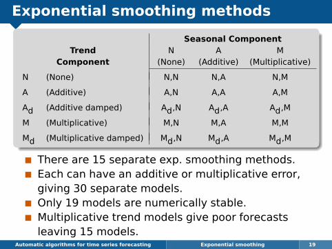
There are 15 separate exp. smoothing methods.
Automatic algorithms for time series forecasting Exponential smoothing 19

Exponential smoothing methods
Seasonal ComponentTrend N A M
Component (None) (Additive) (Multiplicative)
N (None) N,N N,A N,M
A (Additive) A,N A,A A,M
Ad (Additive damped) Ad,N Ad,A Ad,M
M (Multiplicative) M,N M,A M,M
Md (Multiplicative damped) Md,N Md,A Md,M
There are 15 separate exp. smoothing methods.Each can have an additive or multiplicative error,giving 30 separate models.
Automatic algorithms for time series forecasting Exponential smoothing 19

Exponential smoothing methods
Seasonal ComponentTrend N A M
Component (None) (Additive) (Multiplicative)
N (None) N,N N,A N,M
A (Additive) A,N A,A A,M
Ad (Additive damped) Ad,N Ad,A Ad,M
M (Multiplicative) M,N M,A M,M
Md (Multiplicative damped) Md,N Md,A Md,M
There are 15 separate exp. smoothing methods.Each can have an additive or multiplicative error,giving 30 separate models.Only 19 models are numerically stable.
Automatic algorithms for time series forecasting Exponential smoothing 19
Exponential smoothing methods
Seasonal ComponentTrend N A M
Component (None) (Additive) (Multiplicative)
N (None) N,N N,A N,M
A (Additive) A,N A,A A,M
Ad (Additive damped) Ad,N Ad,A Ad,M
M (Multiplicative) M,N M,A M,M
Md (Multiplicative damped) Md,N Md,A Md,M
There are 15 separate exp. smoothing methods.Each can have an additive or multiplicative error,giving 30 separate models.Only 19 models are numerically stable.Multiplicative trend models give poor forecastsleaving 15 models.
Automatic algorithms for time series forecasting Exponential smoothing 19

Exponential smoothing methods
Seasonal ComponentTrend N A M
Component (None) (Additive) (Multiplicative)
N (None) N,N N,A N,M
A (Additive) A,N A,A A,M
Ad (Additive damped) Ad,N Ad,A Ad,M
M (Multiplicative) M,N M,A M,M
Md (Multiplicative damped) Md,N Md,A Md,M
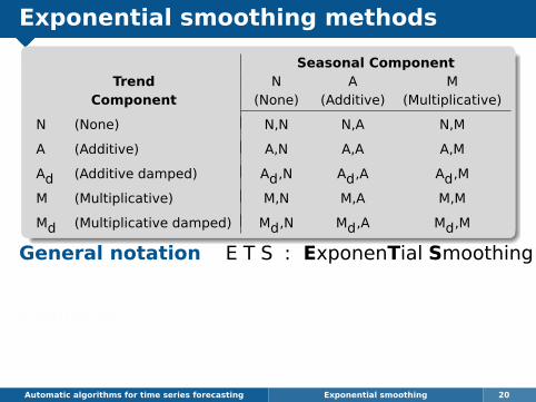
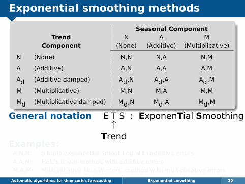
General notation E T S : ExponenTial Smoothing
Examples:A,N,N: Simple exponential smoothing with additive errorsA,A,N: Holt’s linear method with additive errorsM,A,M: Multiplicative Holt-Winters’ method with multiplicative errors
Automatic algorithms for time series forecasting Exponential smoothing 20
Exponential smoothing methods
Seasonal ComponentTrend N A M
Component (None) (Additive) (Multiplicative)
N (None) N,N N,A N,M
A (Additive) A,N A,A A,M
Ad (Additive damped) Ad,N Ad,A Ad,M
M (Multiplicative) M,N M,A M,M
Md (Multiplicative damped) Md,N Md,A Md,M
General notation E T S : ExponenTial Smoothing↑
TrendExamples:
A,N,N: Simple exponential smoothing with additive errorsA,A,N: Holt’s linear method with additive errorsM,A,M: Multiplicative Holt-Winters’ method with multiplicative errors
Automatic algorithms for time series forecasting Exponential smoothing 20

Exponential smoothing methods
Seasonal ComponentTrend N A M
Component (None) (Additive) (Multiplicative)
N (None) N,N N,A N,M
A (Additive) A,N A,A A,M
Ad (Additive damped) Ad,N Ad,A Ad,M
M (Multiplicative) M,N M,A M,M
Md (Multiplicative damped) Md,N Md,A Md,M
General notation E T S : ExponenTial Smoothing↑ ↖
Trend SeasonalExamples:
A,N,N: Simple exponential smoothing with additive errorsA,A,N: Holt’s linear method with additive errorsM,A,M: Multiplicative Holt-Winters’ method with multiplicative errors
Automatic algorithms for time series forecasting Exponential smoothing 20

Exponential smoothing methods
Seasonal ComponentTrend N A M
Component (None) (Additive) (Multiplicative)
N (None) N,N N,A N,M
A (Additive) A,N A,A A,M
Ad (Additive damped) Ad,N Ad,A Ad,M
M (Multiplicative) M,N M,A M,M
Md (Multiplicative damped) Md,N Md,A Md,M
General notation E T S : ExponenTial Smoothing↗ ↑ ↖
Error Trend SeasonalExamples:
A,N,N: Simple exponential smoothing with additive errorsA,A,N: Holt’s linear method with additive errorsM,A,M: Multiplicative Holt-Winters’ method with multiplicative errors
Automatic algorithms for time series forecasting Exponential smoothing 20
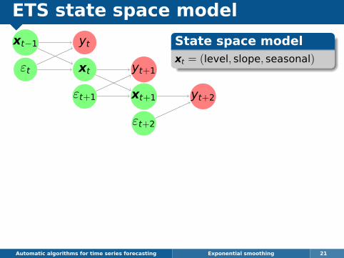
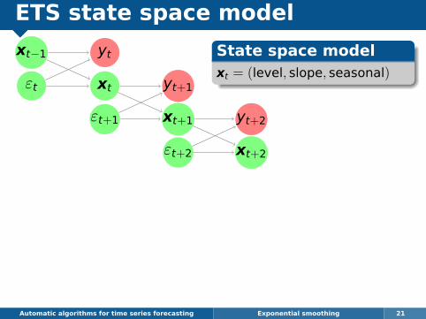
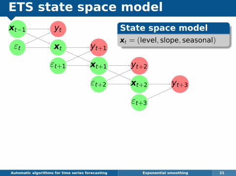
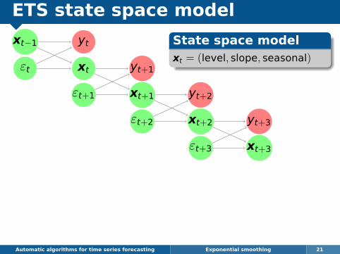
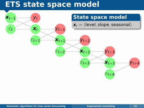
Innovations state space models
å All ETS models can be written in innovationsstate space form (IJF, 2002).
å Additive and multiplicative versions give thesame point forecasts but different predictionintervals.
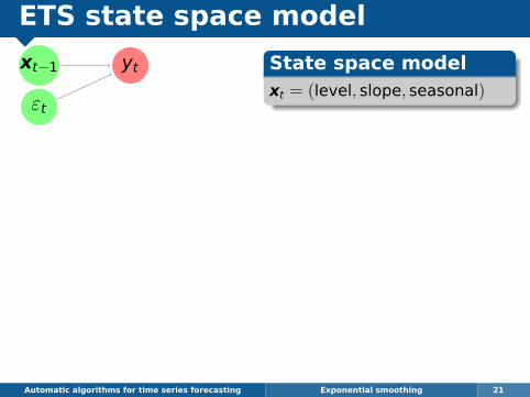
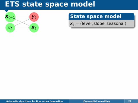
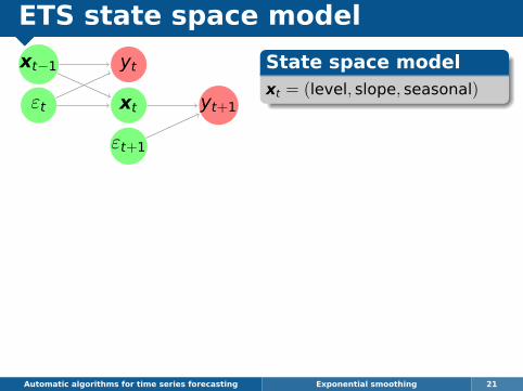
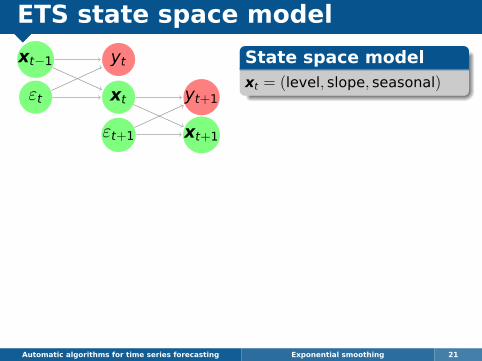
ETS state space model
xt−1
εt
yt
Automatic algorithms for time series forecasting Exponential smoothing 21
State space modelxt = (level, slope, seasonal)
ETS state space model
xt−1
εt
yt
xt
Automatic algorithms for time series forecasting Exponential smoothing 21
State space modelxt = (level, slope, seasonal)
ETS state space model
xt−1
εt
yt
xt yt+1
εt+1
Automatic algorithms for time series forecasting Exponential smoothing 21
State space modelxt = (level, slope, seasonal)
ETS state space model
xt−1
εt
yt
xt yt+1
εt+1 xt+1
Automatic algorithms for time series forecasting Exponential smoothing 21
State space modelxt = (level, slope, seasonal)
ETS state space model
xt−1
εt
yt
xt yt+1
εt+1 xt+1 yt+2
εt+2
Automatic algorithms for time series forecasting Exponential smoothing 21
State space modelxt = (level, slope, seasonal)
ETS state space model
xt−1
εt
yt
xt yt+1
εt+1 xt+1 yt+2
εt+2 xt+2
Automatic algorithms for time series forecasting Exponential smoothing 21
State space modelxt = (level, slope, seasonal)
ETS state space model
xt−1
εt
yt
xt yt+1
εt+1 xt+1 yt+2
εt+2 xt+2 yt+3
εt+3
Automatic algorithms for time series forecasting Exponential smoothing 21
State space modelxt = (level, slope, seasonal)
ETS state space model
xt−1
εt
yt
xt yt+1
εt+1 xt+1 yt+2
εt+2 xt+2 yt+3
εt+3 xt+3
Automatic algorithms for time series forecasting Exponential smoothing 21
State space modelxt = (level, slope, seasonal)
ETS state space model
xt−1
εt
yt
xt yt+1
εt+1 xt+1 yt+2
εt+2 xt+2 yt+3
εt+3 xt+3 yt+4
εt+4
Automatic algorithms for time series forecasting Exponential smoothing 21
State space modelxt = (level, slope, seasonal)

ETS state space model
xt−1
εt
yt
xt yt+1
εt+1 xt+1 yt+2
εt+2 xt+2 yt+3
εt+3 xt+3 yt+4
εt+4
Automatic algorithms for time series forecasting Exponential smoothing 21
State space modelxt = (level, slope, seasonal)
EstimationCompute likelihood L fromε1, ε2, . . . , εT.Optimize L wrt modelparameters.

ETS state space model
xt−1
εt
yt
xt yt+1
εt+1 xt+1 yt+2
εt+2 xt+2 yt+3
εt+3 xt+3 yt+4
εt+4
Automatic algorithms for time series forecasting Exponential smoothing 21
State space modelxt = (level, slope, seasonal)
EstimationCompute likelihood L fromε1, ε2, . . . , εT.Optimize L wrt modelparameters.
Q: How to choosebetween the 15useful ETS models?

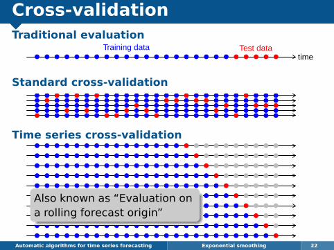
Cross-validationTraditional evaluation
Automatic algorithms for time series forecasting Exponential smoothing 22
● ● ● ● ● ● ● ● ● ● ● ● ● ● ● ● ● ● ● ● ● ● ● ● ● timeTraining data Test data
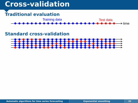
Cross-validationTraditional evaluation
Standard cross-validation
Automatic algorithms for time series forecasting Exponential smoothing 22
● ● ● ● ● ● ● ● ● ● ● ● ● ● ● ● ● ● ● ● ● ● ● ● ● timeTraining data Test data
● ● ● ● ● ● ● ● ● ● ● ● ● ● ● ● ● ● ● ●● ● ●● ●● ● ● ● ● ● ● ● ● ● ● ● ● ● ● ● ● ● ● ●●● ●● ●● ● ● ● ● ● ● ● ● ● ● ● ● ● ● ● ● ● ● ●● ●●● ●● ● ● ● ● ● ● ● ● ● ● ● ● ● ● ● ● ● ● ●●●● ● ●
● ● ● ● ● ● ● ● ● ● ● ● ● ● ● ● ● ● ● ●● ● ●● ●
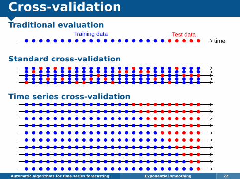
Cross-validationTraditional evaluation
Standard cross-validation
Time series cross-validation
Automatic algorithms for time series forecasting Exponential smoothing 22
● ● ● ● ● ● ● ● ● ● ● ● ● ● ● ● ● ● ● ● ● ● ● ● ● timeTraining data Test data
● ● ● ● ● ● ● ● ● ● ● ● ● ● ● ● ● ● ● ●● ● ●● ●● ● ● ● ● ● ● ● ● ● ● ● ● ● ● ● ● ● ● ●●● ●● ●● ● ● ● ● ● ● ● ● ● ● ● ● ● ● ● ● ● ● ●● ●●● ●● ● ● ● ● ● ● ● ● ● ● ● ● ● ● ● ● ● ● ●●●● ● ●
● ● ● ● ● ● ● ● ● ● ● ● ● ● ● ● ● ● ● ●● ● ●● ●
● ● ● ● ● ● ● ● ● ● ● ● ● ● ● ● ● ● ● ● ● ● ● ● ●
● ● ● ● ● ● ● ● ● ● ● ● ● ● ● ● ● ● ● ● ● ● ● ● ●
● ● ● ● ● ● ● ● ● ● ● ● ● ● ● ● ● ● ● ● ● ● ● ● ●
● ● ● ● ● ● ● ● ● ● ● ● ● ● ● ● ● ● ● ● ● ● ● ● ●
● ● ● ● ● ● ● ● ● ● ● ● ● ● ● ● ● ● ● ● ● ● ● ● ●
● ● ● ● ● ● ● ● ● ● ● ● ● ● ● ● ● ● ● ● ● ● ● ● ●
● ● ● ● ● ● ● ● ● ● ● ● ● ● ● ● ● ● ● ● ● ● ● ● ●
● ● ● ● ● ● ● ● ● ● ● ● ● ● ● ● ● ● ● ● ● ● ● ● ●
● ● ● ● ● ● ● ● ● ● ● ● ● ● ● ● ● ● ● ● ● ● ● ● ●
● ● ● ● ● ● ● ● ● ● ● ● ● ● ● ● ● ● ● ● ● ● ● ● ●
Also known as “Evaluation ona rolling forecast origin”

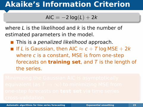
Akaike’s Information Criterion
AIC = −2 log(L) + 2k
where L is the likelihood and k is the number ofestimated parameters in the model.
This is a penalized likelihood approach.If L is Gaussian, then AIC ≈ c + T log MSE + 2kwhere c is a constant, MSE is from one-stepforecasts on training set, and T is the length ofthe series.
Minimizing the Gaussian AIC is asymptoticallyequivalent (as T →∞) to minimizing MSE fromone-step forecasts on test set via time seriescross-validation.Automatic algorithms for time series forecasting Exponential smoothing 23

Akaike’s Information Criterion
AIC = −2 log(L) + 2k
Corrected AICFor small T, AIC tends to over-fit. Bias-correctedversion:
AICC = AIC + 2(k+1)(k+2)T−k
CV-MSE too time consuming for most automaticforecasting purposes. Also requires large T.AICc asymptotically equivalent, can be used onsmall samples and is very fast to compute.
Automatic algorithms for time series forecasting Exponential smoothing 24

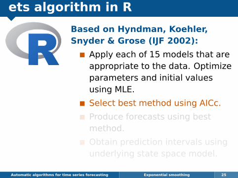
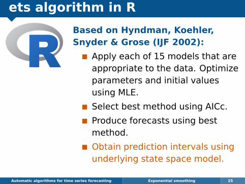
ets algorithm in R
Automatic algorithms for time series forecasting Exponential smoothing 25
Based on Hyndman, Koehler,Snyder & Grose (IJF 2002):
Apply each of 15 models that areappropriate to the data. Optimizeparameters and initial valuesusing MLE.
Select best method using AICc.
Produce forecasts using bestmethod.
Obtain prediction intervals usingunderlying state space model.

Exponential smoothing
Automatic algorithms for time series forecasting Exponential smoothing 26
Forecasts from ETS(M,A,N)
Year
mill
ions
of s
heep
1960 1970 1980 1990 2000 2010
300
400
500
600

Exponential smoothing
fit <- ets(livestock)fcast <- forecast(fit)plot(fcast)
Automatic algorithms for time series forecasting Exponential smoothing 27
Forecasts from ETS(M,A,N)
Year
mill
ions
of s
heep
1960 1970 1980 1990 2000 2010
300
400
500
600

Exponential smoothing
Automatic algorithms for time series forecasting Exponential smoothing 28
Forecasts from ETS(M,N,M)
Year
Tota
l scr
ipts
(m
illio
ns)
1995 2000 2005 2010
0.4
0.6
0.8
1.0
1.2
1.4
1.6

Exponential smoothing
fit <- ets(h02)fcast <- forecast(fit)plot(fcast)
Automatic algorithms for time series forecasting Exponential smoothing 29
Forecasts from ETS(M,N,M)
Year
Tota
l scr
ipts
(m
illio
ns)
1995 2000 2005 2010
0.4
0.6
0.8
1.0
1.2
1.4
1.6

Exponential smoothing
> fitETS(M,N,M)
Smoothing parameters:alpha = 0.4597gamma = 1e-04
Initial states:l = 0.4501s = 0.8628 0.8193 0.7648 0.7675 0.6946 1.2921
1.3327 1.1833 1.1617 1.0899 1.0377 0.9937
sigma: 0.0675
AIC AICc BIC-115.69960 -113.47738 -69.24592
Automatic algorithms for time series forecasting Exponential smoothing 30

M3 comparisons
Method MAPE sMAPE MASE
Theta 17.42 12.76 1.39
ForecastPro 18.00 13.06 1.47
ForecastX 17.35 13.09 1.42
Automatic ANN 17.18 13.98 1.53
B-J automatic 19.13 13.72 1.54
ETS 17.38 13.13 1.43
Automatic algorithms for time series forecasting Exponential smoothing 31
Exponential smoothing
Automatic algorithms for time series forecasting Exponential smoothing 32
Exponential smoothing
Automatic algorithms for time series forecasting Exponential smoothing 32
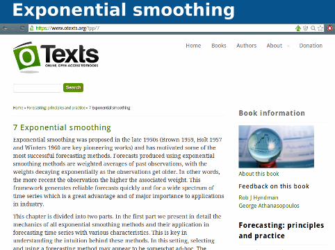
www.OTexts.org/fpp
Exponential smoothing
Automatic algorithms for time series forecasting Exponential smoothing 32

Exercise
1 Use ets to find the best ETS models for thefollowing series: ibmclose, eggs, bricksq,hsales.
2 Try ets with cangas and lynx. What do youlearn?
3 Can you find another series for which ets givesbad forecasts?
Automatic algorithms for time series forecasting Exponential smoothing 33
Outline
1 Forecasting competitions
2 Exponential smoothing
3 ARIMA modelling
4 Automatic nonlinear forecasting?
5 Time series with complex seasonality
6 Recent developments
Automatic algorithms for time series forecasting ARIMA modelling 34
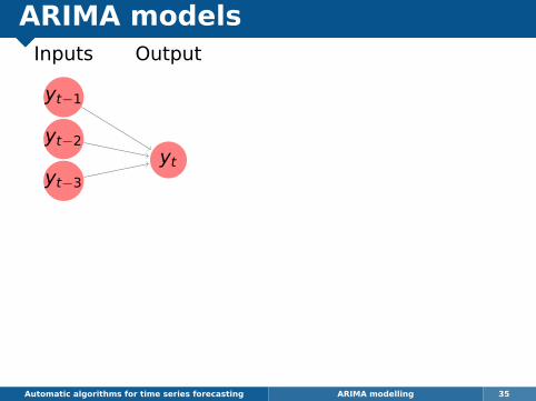
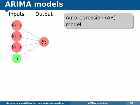
ARIMA models
yt−1
yt−2
yt−3
yt
Inputs Output
Automatic algorithms for time series forecasting ARIMA modelling 35
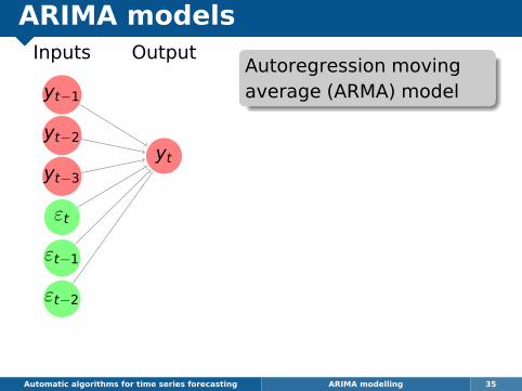
ARIMA models
yt−1
yt−2
yt−3
εt
yt
Inputs Output
Automatic algorithms for time series forecasting ARIMA modelling 35
Autoregression (AR)model
ARIMA models
yt−1
yt−2
yt−3
εt
εt−1
εt−2
yt
Inputs Output
Automatic algorithms for time series forecasting ARIMA modelling 35
Autoregression movingaverage (ARMA) model
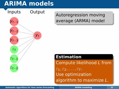
ARIMA models
yt−1
yt−2
yt−3
εt
εt−1
εt−2
yt
Inputs Output
Automatic algorithms for time series forecasting ARIMA modelling 35
Autoregression movingaverage (ARMA) model
EstimationCompute likelihood L fromε1, ε2, . . . , εT.Use optimizationalgorithm to maximize L.

ARIMA models
yt−1
yt−2
yt−3
εt
εt−1
εt−2
yt
Inputs Output
Automatic algorithms for time series forecasting ARIMA modelling 35
Autoregression movingaverage (ARMA) model
EstimationCompute likelihood L fromε1, ε2, . . . , εT.Use optimizationalgorithm to maximize L.
ARIMA modelAutoregression movingaverage (ARMA) modelapplied to differences.

ARIMA modelling
Automatic algorithms for time series forecasting ARIMA modelling 36
Auto ARIMA
Automatic algorithms for time series forecasting ARIMA modelling 37
Forecasts from ARIMA(0,1,0) with drift
Year
mill
ions
of s
heep
1960 1970 1980 1990 2000 2010
250
300
350
400
450
500
550

Auto ARIMA
fit <- auto.arima(livestock)fcast <- forecast(fit)plot(fcast)
Automatic algorithms for time series forecasting ARIMA modelling 38
Forecasts from ARIMA(0,1,0) with drift
Year
mill
ions
of s
heep
1960 1970 1980 1990 2000 2010
250
300
350
400
450
500
550
Auto ARIMA
Automatic algorithms for time series forecasting ARIMA modelling 39
Forecasts from ARIMA(3,1,3)(0,1,1)[12]
Year
Tota
l scr
ipts
(m
illio
ns)
1995 2000 2005 2010
0.4
0.6
0.8
1.0
1.2
1.4

Auto ARIMA
fit <- auto.arima(h02)fcast <- forecast(fit)plot(fcast)
Automatic algorithms for time series forecasting ARIMA modelling 40
Forecasts from ARIMA(3,1,3)(0,1,1)[12]
Year
Tota
l scr
ipts
(m
illio
ns)
1995 2000 2005 2010
0.4
0.6
0.8
1.0
1.2
1.4

Auto ARIMA
> fitSeries: h02ARIMA(3,1,3)(0,1,1)[12]
Coefficients:ar1 ar2 ar3 ma1 ma2 ma3 sma1
-0.3648 -0.0636 0.3568 -0.4850 0.0479 -0.353 -0.5931s.e. 0.2198 0.3293 0.1268 0.2227 0.2755 0.212 0.0651
sigma^2 estimated as 0.002706: log likelihood=290.25AIC=-564.5 AICc=-563.71 BIC=-538.48
Automatic algorithms for time series forecasting ARIMA modelling 41
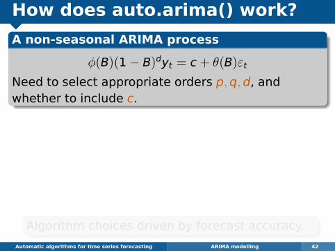
How does auto.arima() work?
A non-seasonal ARIMA process
φ(B)(1− B)dyt = c + θ(B)εt
Need to select appropriate orders p,q,d, andwhether to include c.
Automatic algorithms for time series forecasting ARIMA modelling 42
Algorithm choices driven by forecast accuracy.

How does auto.arima() work?
A non-seasonal ARIMA process
φ(B)(1− B)dyt = c + θ(B)εt
Need to select appropriate orders p,q,d, andwhether to include c.
Hyndman & Khandakar (JSS, 2008) algorithm:Select no. differences d via KPSS unit root test.Select p,q, c by minimising AICc.Use stepwise search to traverse model space,starting with a simple model and consideringnearby variants.
Automatic algorithms for time series forecasting ARIMA modelling 42
Algorithm choices driven by forecast accuracy.
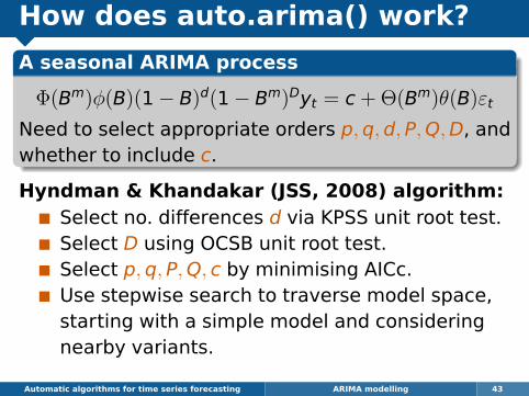
How does auto.arima() work?
A seasonal ARIMA process
Φ(Bm)φ(B)(1− B)d(1− Bm)Dyt = c + Θ(Bm)θ(B)εt
Need to select appropriate orders p,q,d, P,Q,D, andwhether to include c.
Hyndman & Khandakar (JSS, 2008) algorithm:Select no. differences d via KPSS unit root test.Select D using OCSB unit root test.Select p,q, P,Q, c by minimising AICc.Use stepwise search to traverse model space,starting with a simple model and consideringnearby variants.
Automatic algorithms for time series forecasting ARIMA modelling 43
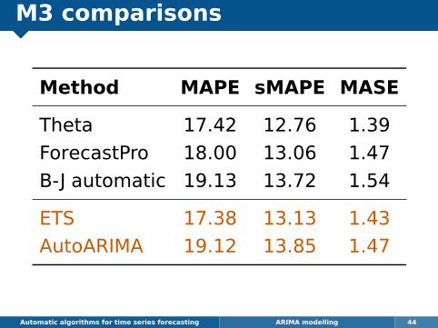
M3 comparisons
Method MAPE sMAPE MASE
Theta 17.42 12.76 1.39
ForecastPro 18.00 13.06 1.47
B-J automatic 19.13 13.72 1.54
ETS 17.38 13.13 1.43
AutoARIMA 19.12 13.85 1.47
Automatic algorithms for time series forecasting ARIMA modelling 44

Exercise
1 Use auto.arima to find the best ARIMA modelsfor the following series: ibmclose, eggs,bricksq, hsales.
2 Try auto.arima with cangas and lynx. What doyou learn?
3 Can you find a series for which auto.arimagives bad forecasts?
4 How would you compare the ETS and ARIMAresults?
Automatic algorithms for time series forecasting ARIMA modelling 45
Outline
1 Forecasting competitions
2 Exponential smoothing
3 ARIMA modelling
4 Automatic nonlinear forecasting?
5 Time series with complex seasonality
6 Recent developments
Automatic algorithms for time series forecasting Automatic nonlinear forecasting? 46
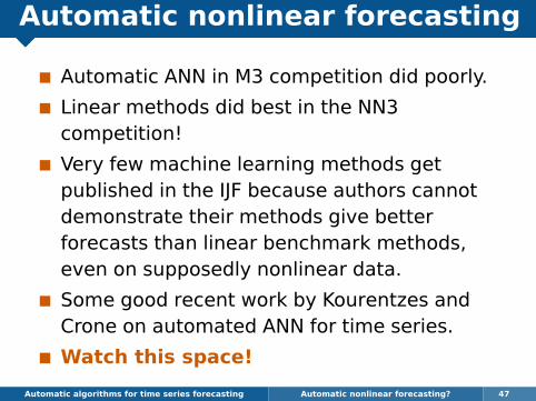
Automatic nonlinear forecasting
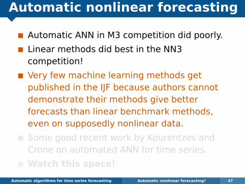
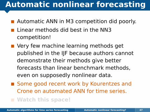
Automatic ANN in M3 competition did poorly.
Linear methods did best in the NN3competition!
Very few machine learning methods getpublished in the IJF because authors cannotdemonstrate their methods give betterforecasts than linear benchmark methods,even on supposedly nonlinear data.
Some good recent work by Kourentzes andCrone on automated ANN for time series.
Watch this space!
Automatic algorithms for time series forecasting Automatic nonlinear forecasting? 47

Automatic nonlinear forecasting
Automatic ANN in M3 competition did poorly.
Linear methods did best in the NN3competition!
Very few machine learning methods getpublished in the IJF because authors cannotdemonstrate their methods give betterforecasts than linear benchmark methods,even on supposedly nonlinear data.
Some good recent work by Kourentzes andCrone on automated ANN for time series.
Watch this space!
Automatic algorithms for time series forecasting Automatic nonlinear forecasting? 47
Outline
1 Forecasting competitions
2 Exponential smoothing
3 ARIMA modelling
4 Automatic nonlinear forecasting?
5 Time series with complex seasonality
6 Recent developments
Automatic algorithms for time series forecasting Time series with complex seasonality 48

Examples
Automatic algorithms for time series forecasting Time series with complex seasonality 49
US finished motor gasoline products
Weeks
Tho
usan
ds o
f bar
rels
per
day
1992 1994 1996 1998 2000 2002 2004
6500
7000
7500
8000
8500
9000
9500

Examples
Automatic algorithms for time series forecasting Time series with complex seasonality 49
Number of calls to large American bank (7am−9pm)
5 minute intervals
Num
ber
of c
all a
rriv
als
100
200
300
400
3 March 17 March 31 March 14 April 28 April 12 May
Examples
Automatic algorithms for time series forecasting Time series with complex seasonality 49
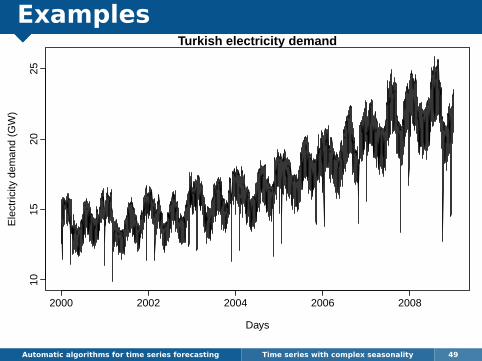
Turkish electricity demand
Days
Ele
ctric
ity d
eman
d (G
W)
2000 2002 2004 2006 2008
1015
2025

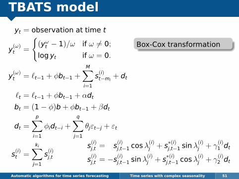
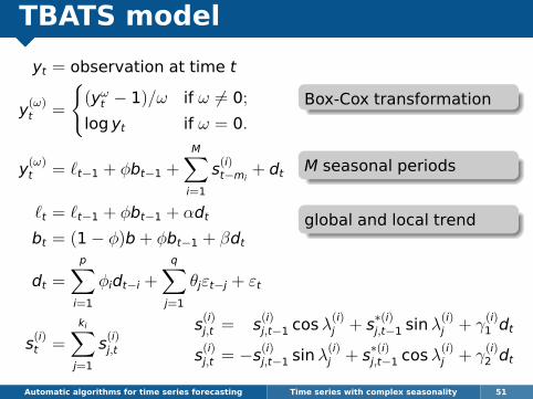
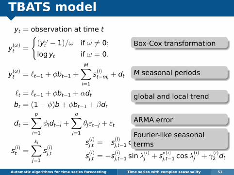
TBATS model
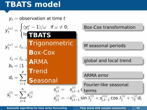
TBATSTrigonometric terms for seasonality
Box-Cox transformations for heterogeneity
ARMA errors for short-term dynamics
Trend (possibly damped)
Seasonal (including multiple and non-integer periods)
Automatic algorithm described in AM De Livera,RJ Hyndman, and RD Snyder (2011). “Forecastingtime series with complex seasonal patterns usingexponential smoothing”. Journal of the AmericanStatistical Association 106(496), 1513–1527.
Automatic algorithms for time series forecasting Time series with complex seasonality 50

TBATS model
yt = observation at time t
y(ω)t =
{(yωt − 1)/ω if ω 6= 0;
log yt if ω = 0.
y(ω)t = `t−1 + φbt−1 +M∑i=1
s(i)t−mi+ dt
`t = `t−1 + φbt−1 + αdt
bt = (1− φ)b + φbt−1 + βdt
dt =
p∑i=1
φidt−i +
q∑j=1
θjεt−j + εt
s(i)t =
ki∑j=1
s(i)j,t
Automatic algorithms for time series forecasting Time series with complex seasonality 51
s(i)j,t = s(i)j,t−1 cosλ(i)j + s∗(i)j,t−1 sinλ(i)j + γ(i)1 dt
s(i)j,t = −s(i)j,t−1 sinλ(i)j + s∗(i)j,t−1 cosλ(i)j + γ(i)2 dt
Box-Cox transformation
M seasonal periods
global and local trend
ARMA error
Fourier-like seasonalterms
TBATSTrigonometric
Box-Cox
ARMA
Trend
Seasonal
Examples
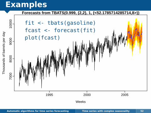
fit <- tbats(gasoline)fcast <- forecast(fit)plot(fcast)
Automatic algorithms for time series forecasting Time series with complex seasonality 52
Forecasts from TBATS(0.999, {2,2}, 1, {<52.1785714285714,8>})
Weeks
Tho
usan
ds o
f bar
rels
per
day
1995 2000 2005
7000
8000
9000
1000
0
Examples
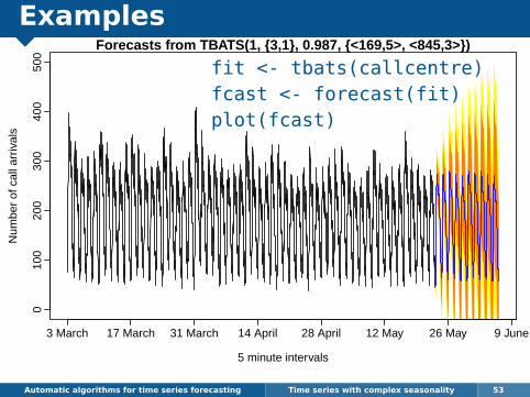
fit <- tbats(callcentre)fcast <- forecast(fit)plot(fcast)
Automatic algorithms for time series forecasting Time series with complex seasonality 53
Forecasts from TBATS(1, {3,1}, 0.987, {<169,5>, <845,3>})
5 minute intervals
Num
ber
of c
all a
rriv
als
010
020
030
040
050
0
3 March 17 March 31 March 14 April 28 April 12 May 26 May 9 June
Examples
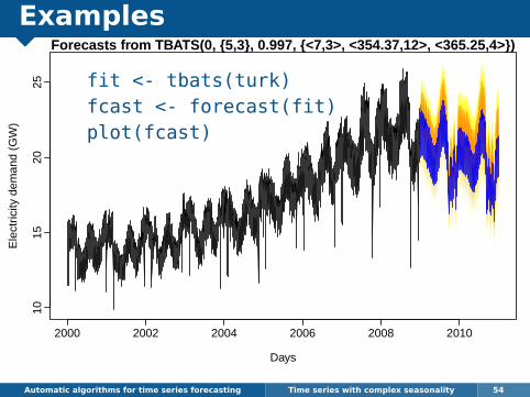
fit <- tbats(turk)fcast <- forecast(fit)plot(fcast)
Automatic algorithms for time series forecasting Time series with complex seasonality 54
Forecasts from TBATS(0, {5,3}, 0.997, {<7,3>, <354.37,12>, <365.25,4>})
Days
Ele
ctric
ity d
eman
d (G
W)
2000 2002 2004 2006 2008 2010
1015
2025

Outline
1 Forecasting competitions
2 Exponential smoothing
3 ARIMA modelling
4 Automatic nonlinear forecasting?
5 Time series with complex seasonality
6 Recent developments
Automatic algorithms for time series forecasting Recent developments 55
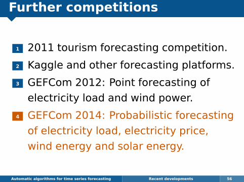
Further competitions
1 2011 tourism forecasting competition.
2 Kaggle and other forecasting platforms.
3 GEFCom 2012: Point forecasting of
electricity load and wind power.
4 GEFCom 2014: Probabilistic forecasting
of electricity load, electricity price,
wind energy and solar energy.
Automatic algorithms for time series forecasting Recent developments 56
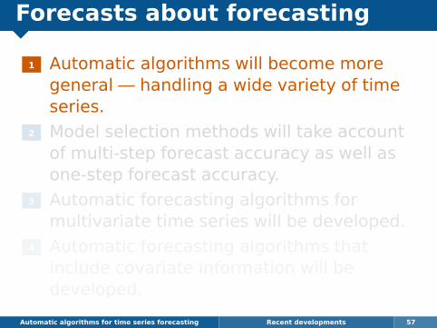
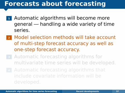
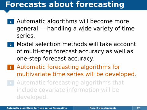
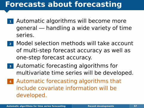
Forecasts about forecasting
1 Automatic algorithms will become moregeneral — handling a wide variety of timeseries.
2 Model selection methods will take accountof multi-step forecast accuracy as well asone-step forecast accuracy.
3 Automatic forecasting algorithms formultivariate time series will be developed.
4 Automatic forecasting algorithms thatinclude covariate information will bedeveloped.
Automatic algorithms for time series forecasting Recent developments 57