Roads and Poverty in Rural Laos*

Peter Warr

Australian National University

February 2006

Abstract

The relationship between poverty incidence and road development is analyzed

in this paper, in the context of rural Laos. The results indicate that improving

road access is an effective way of reducing rural poverty. Between 1997-98 and

2002-03, rural poverty incidence in Laos declined by almost on tenth of the

rural population. Over this same period road improvement was significant,

providing all-season access to many areas previously having only dry season

access. The analysis provided in this paper suggests that about 13 per cent of

the poverty reduction can be attributed to improvements in road access.

JEL classifications: H53; I32; O53; R41

Key words: Asia; Laos; poverty incidence; rural roads.

Address: Division of Economics, RSPAS, Australian National University, Canberra, ACT 2601, Australia Telephone: 61 2 6125 2682. Fax: 61 2 6125 3700 Email: Peter.Warr@anu.edu.au

* Contributed paper to the Australian Agricultural and Resource Economics Society Annual Conference, Sydney, 8-10 February 2006. Excellent research assistance was provided by Edda Claus, Chanthalath Pongmala and Arief Ramayandi. Data were provided through the cooperation of the National Statistical Center (NSC), Vientiane. The kind assistance of the staff of NSC and Hans Petterson of Statistics Sweden in interpreting these data is gratefully acknowledged. Helpful comments were also received from John Weiss and Meng Xin. The author is responsible for all defects.

2

1. Introduction

In less developed countries most poor people live in rural areas, where they often experience

low standards of public infrastructure, especially roads. Bad roads raise transport costs,

limiting the use poor people can make of local markets to sell their produce, purchase

consumer goods and obtain off-farm employment. Access to educational and health facilities,

where they exist, is also constrained when it is difficult to reach them. In tropical areas,

unsealed roads may actually be impassable during the extended rainy periods of the year.

These problems are particularly acute in Lao PDR (subsequently Laos), where inadequate

roads are a severe problem for rural people. Action to improve rural roads therefore seems a

likely means by which large numbers of people might acquire the opportunity to participate in

the market economy and thereby raise themselves out of poverty. Significant road

improvement has occurred in Laos over the last decade. But does it actually reduce poverty?

This paper is an attempt to study the contribution that improved rural roads have made to

poverty reduction in Laos in the recent past and - by extension - the scope for continued

poverty reduction through this means.

Significant road improvement is generally not a form of investment that rural people can

make by themselves. Public sector involvement is required. This necessity arises from

economies of scale in the provision of these goods and because they tend to be public or

partially public goods. The first feature implies that when they are provided on an exclusively

private basis, monopolies result. The second feature implies that when goods of this kind are

provided by the private sector, they are under-provided. Because private sector investors are

unable to capture the benefits that the investments generate, they may invest little or nothing

in forms of infrastructure which generate large social returns.

A number of studies have suggested that improvement of infrastructure in rural areas can

contribute to agricultural productivity and economic welfare in those areas. Examples include

3

Binswanger et al. (1993), van de Walle and Nead (1995), van de Walle (1996 and 2002),

Jacoby (2000) and Gibson and Rozelle (2003). Lanjouw (1999) demonstrates, for the case of

Ecuador, the importance of access to off-farm employment in these outcomes. A study of rural

China (Jalan and Ravallion 1998) suggested that higher density of roads in a particular area

lowered the probability that households in that area would be poor. Srinivasan (1986) points

to the special importance of these issues in landlocked countries such as Laos.

Jacoby (2000) is particularly relevant, in part because of the similarity between Nepal and

Laos. She studies the effects of rural roads on rural incomes in Nepal using household survey

data. The income effect of road access is decomposed into a return to land and a return to labor.

The results confirm that both real land prices and real wages are raised by road development.

The net effect is slightly progressive with respect to income. Households with lower real

incomes initially, who tend on average to be furthest from the markets, receive the largest

proportional income gain from improved roads, although this progressive element was minor.

These results imply that rural road improvement is an effective instrument reducing absolute

poverty incidence but not an effective way of reducing income inequality.

Suppose it is found that areas with better access to main roads had higher levels of

consumption expenditures per person and lower levels of poverty incidence. This does not in

itself prove that improved roads cause lower levels of poverty, for two kinds of reasons. First,

the regions with better roads (and lower poverty incidence) differ from those with inferior

roads (and higher poverty incidence) in many respects, not just the quality of roads.

Multivariate regression is a statistical device for dealing with this problem, by allowing for the

levels of other variables such as education, health facilities and regional effects. If a positive

association is still found between access to roads and per capita consumption, then this point

has been allowed for.

A second problem is that if better-off areas are favored by the government for the

construction of these infrastructure facilities, then the existence of a correlation between their

provision and the economic indicator concerned may not reveal that the provision of the

4

infrastructure causes better economic performance, but rather the reverse. Studies noting this

potential problem, now known as the ‘endogenous placement’ problem include Binswanger et

al. (1993), and van der Walle and Nead (1995). For this reason, wherever possible it is

desirable to supplement such cross-sectional analyses with studies over time which focus on

the effect that changes in road provision over time have on changes in economic indicators,

like poverty incidence, income, expenditure and so forth.

The structure of this paper is as follows. Section 2 briefly reviews economic change in

Laos since the late 1980s. This is important because this paper is concerned with analyzing

changes in rural poverty incidence between 1997-98 and 2002-03. Due to structural changes

within the Lao economy, rural areas have been subjected to considerable economic pressure,

and this is relevant for understanding the changes in poverty incidence that have occurred.

Section 3 then presents the results of the empirical analysis of the relationship between road

development and poverty incidence in rural areas of Laos using household survey data.

Section 4 concludes.

2. Economic Background

Output

Laos is an especially poor country, with GDP per person in 2002 at US$ 310, and total GDP

of US$ 1.7 billion. From 1991 to 2002 annual growth of GDP averaged 6.2 per cent per

annum (Figure 1), or around 3.8 per cent per person. The agricultural sector dominates

employment, with 80 per cent of the workforce and it contributes about 50 per cent of GDP.

Laos remains dependent on external support. In 2002/3 external donors contributed 61 per cent

of the government’s capital budget, representing 39 per cent of total public expenditure, and

7.6 per cent of GDP. Structural change within the Lao economy has been significant. The

agricultural sector contracted from 61 per cent of GDP in 1990 to 50 per cent in 2002. Most of

this contraction occurred in crops, especially in rice, and this contraction was concentrated in

5

the first half of the 1990s, when crops’ share of GDP fell from 37 to 25 per cent. From then

until the present, the share of the crops sector recovered to around 30 per cent of GDP. Heavy

public investment in irrigation in the second half of the 1990s accounted for this change.

One feature of the changes in the crop sector is important. The total area planted to rice

remained virtually unchanged from 1990 to 2000, but within this the irrigated rice sector

expanded very markedly, responding to the irrigation investments mentioned above, and the

upland rice area (non-irrigated) contracted by 70 per cent. Rice became a less attractive

activity for upland people. To some extent this was due to the availability of alternative crops

with market outlets both within Laos and in neighboring countries, partly to the relaxed

insistence from the government that all regions of the country strive for rice self-sufficiency,

but it was also due to the declining profitability of rice itself, reflecting relative price

movements within the country.

Prices

Inflation was moderate through the first half of the 1990s, at single digit levels for most of this

period. It accelerated from 1998 to 2000, peaking at 142 per cent in 1999 (Figure 1). This

inflationary surge was related to agricultural policy. The government of Laos is committed to a

goal of rice self-sufficiency. However, it was apparent through the first half of the 1990s that

rice output was not growing as fast as population. A large public investment in irrigation

facilities followed, beginning in 1996-97, producing large public sector deficits, especially in

1998-99. But the deficits were financed to a considerable extent by monetary creation,

producing the inflation and currency depreciation of the late 1990s. Since 2001 consumer

price inflation has been contained, with an average annual rate just under 10 per cent. The

inflation in consumer prices in the late 1990s coincided with a collapse of the exchange rate.

The kip / dollar rate collapsed from roughly 2,000 at the end of 1997 to 8,200 at the end of

2001.

6

The macroeconomic events described above produced significant relative price changes

within Laos. They are summarized in Figure 2. Because producer prices are unavailable, this

figure draws on consumer price data to show a decline in food prices relative to services

prices. These data tell a clear story. Agricultural commodity prices declined markedly relative

to non-agricultural prices, especially those of services and construction. An economic boom

followed the more open economic environment created by the reforms, but this boom was

concentrated in the services and construction sectors, which drew resources from elsewhere,

especially from agriculture.

Economic reforms

Economic reforms, beginning around 1987, contributed to these macroeconomic

outcomes. The reforms, officially called the New Economic Mechanism (NEM), mainly took

the form of removing prohibitions on market activity, permitting greater participation in both

local markets and markets in neighboring countries. The program had indirect effects on

agricultural output, which were in some cases negative. The reforms were accompanied by

increased inflows of foreign aid and foreign investment. The increased domestic expenditure

made possible by these capital inflows produced demand-side effects that implied contraction

of agriculture.

Increased demand increased the domestic prices of those goods and services that could

not readily be imported, including most services and construction. The resulting expansion of

these sectors attracted resources, including labor, away from agriculture. This phenomenon –

the ‘Dutch Disease’ or ‘booming sector’ effect – has been observed in many countries

experiencing large increases in capital or export revenue inflows from abroad. It causes the

prices of agricultural and other traded commodities to decline relative to other prices, with

negative effects on agricultural production. To the extent that the NEM increased the exposure

of agricultural commodities to international markets, this policy change indirectly increased

the impact that these market phenomena had on agricultural production.

7

From 1997 to 1999 this real appreciation was reversed by the massive nominal

depreciation mentioned above. A depreciation increases the nominal (domestic currency)

prices of traded goods. Some stickiness in non-traded goods prices caused them to respond

slowly to the monetary expansion that was occurring at the same time, with the result that the

ratio of traded to non-traded goods prices increased. This effect ceased after 2000 and real

appreciation resumed.

The relevance of these events is that since around 1990 agricultural producers in Laos

have been subject to a considerable cost-price squeeze. This phenomenon has accelerated the

rate of rural to urban migration that would otherwise have occurred. The deterioration in the

profitability of agricultural production for the market has also impeded the entry into the

market economy of subsistence agricultural producers. In short, these events have resulted in

higher levels of rural poverty incidence than might otherwise have occurred. This background

is important for understanding rural poverty in Laos.

Poverty

Studies of poverty incidence in Laos are constrained by the availability of household

survey data sets which can support this form of analysis. The only such data sets available are

assembled by the government’s National Statistical Center and are known as the Lao

Expenditure and Consumption Survey (LECS). Three such surveys have been conducted to

date:

LECS 1, covering 1992-93;

LECS 2 covering 1997-98; and

LECS 3, covering 2002-03.

According to these surveys, poverty incidence at the national level declined from 46 per

cent of the population in 1992-93 to 39 per cent in 1997-98 and then to 31 per cent in 2002-03

(Table 1). These data are based on comparisons of household expenditures (rather than

incomes) with an official poverty line adjusted over time to hold real purchasing power

8

constant.1 As in most developing countries, poverty in Laos is concentrated in rural areas. The

percentage of the rural population with consumption expenditures below the official poverty

line has been estimated at 52, 43 and 33 per cent, respectively, over the same years. The

corresponding estimates for poverty incidence in urban areas were 27, 22 and 23 per cent,

respectively. Data from the LECS surveys indicate that in 2002-03, 77 per cent of the Lao

population resided in rural areas, but poverty incidence in rural areas (the proportion of the

rural population with real expenditures below the poverty line) was almost double that of

urban areas. Most tellingly, rural areas accounted for 86.5 per cent of all poor people.2

Changes in statistical measures adopted at the time of the LECS 2 survey limit the scope

for detailed comparison with LECS 1, but LECS 2 and 3 are closely comparable. Earlier

poverty assessment studies for Laos, using the LECS 2 data set, confirm that in 1997-98 areas

with better access to main roads had higher levels of consumption expenditures per person,

allowing for the levels of other variables such as education, health facilities and regional

effects. Two important examples are Datt and Wang (2001) and Kakwani, et al. (2002). In

each of these studies, the relationship between infrastructure and real expenditures is only one

of many issues examined and this effect of road infrastructure occupies a minor part in the

analysis and discussion. Neither estimates the implications of the results for poverty incidence

and neither recognizes the possible relevance of the ‘endogenous placement’ effect.

Consequently, it is not clear whether the reported correlation between good roads and

economic welfare means that better roads reduce poverty or merely that richer areas receive

improved roads ahead of poorer areas.

The release of LECS 3 data means that a richer analysis of the relationship between

infrastructure provision and poverty incidence is now possible, by comparing LECS 2 and

1 Among Southeast Asian countries, Indonesia, Cambodia and Vietnam also use household expenditures for this

purpose, but Thailand, Malaysia and the Philippines use household incomes.

2 It can readily be shown that the share of rural areas in the total number of poor people is given by sR

P =αR PR /P , where αR is the share of the total population residing in rural areas, PR is the share of the rural population that is poor (that is, the headcount measure of poverty incidence in rural areas) and P is the share of the total population that is poor.

9

LECS 3, which span an interval (1997-98 to 2002-03) during which there was significant

progress in road provision. That is, the LECS 3 data make it possible to focus to focus on the

determinants of changes in poverty incidence over time, rather than simply the level of poverty

incidence at a particular time.

The present study focuses on the LECS 2 and 3 surveys, summarized in Table 2. The

1997-98 survey (LECS 2) covered 8,882 households containing 57,624 individuals. The data

collection ran from March 1997 to February 1998 with about the same number of households

(about 740) interviewed each month. The timing is important because as the discussion above

indicates, the survey was conducted at a time of high inflation, which reached annual rates

well over 100 per cent. The data on consumption expenditures were collected in current prices,

making the deflation of these expenditures into constant price terms particularly important. Of

the 8,882 households covered, 6,874 were rural and the remaining 2,008 urban. In this study,

only the data relating to rural households are used.

The 2002-03 survey (LECS 3) covered 8,092 households containing 49,790 individuals

with the data collection extending from March 2002 to February 2003. Of these households

6,488 were rural and the remaining 1,604 were urban. Of course, these are sample surveys, not

censuses. The number of households sampled is about 1.2 per cent of the total number of

households within Laos, and the individual households sampled in each survey are seldom the

same. In any case, households are not identified individually and it is therefore not possible to

compare the same households across LECS 2 and LECS 3.

3. Roads and Poverty

10

We now turn to the estimation of the effects that road development has on poverty in rural

Laos. Nominal consumption expenditures per household member were deflated to December

1999 prices using monthly provincial consumer price index data, thus taking account of the

specific month in which the data were collected. This is especially important in the case of

LECS 2, because of the rapid inflation of that time. Multiple regression was used, with the

dependent variable the natural logarithm of real per capita expenditure. The independent

variables are listed in Tables 3 and 4.

The treatment of the dummy variables for dry season access to roads and wet season

access needs explanation. Dummy variables D and W were used, where D takes the value 0 if

the household reports no dry season access and 1 if it reports road access. Then, W is defined

similarly for wet season access. There was no household for which D was zero and W was 1.

With respect to road access there were therefore three categories of households:

(i) no road access at all: D = 0, W = 0;

(ii) access in dry season but not wet season: D = 1, W = 0; and

(iii) access in both seasons: D = 1, W = 1.

The numbers of households belonging to each of these categories are summarized in

Table 2. In LECS 2, 31 per cent of households belonged to category (i) and this barely

changed in LECS 3. These are the most isolated households of the country and according to

these data little progress was made in providing them with road access over this period. In

category (ii) – dry season access but not wet season access – the proportion declined from 28

per cent in LECS 2 to 16 per cent in LECS 3. Thus the number of households which had wet

season access as well as dry season access increased between these two surveys by 12 per cent

of all households. In LECS 3, 52 per cent of all household had year-round road access.

The estimated regression equation handled this combination of outcomes through an

interaction term. The right hand side variables thus included the terms αD+ βD.W ,

11

where α and β are estimated coefficients. In case (i) above D and D.W are both 0. In case (ii)

D = 1 and D.W = 0. In case (iii) D and D.W are both 1. The effect of dry season access alone is

given by α and (noting that whenever W = 1, D = 1 also) the combined effect of dry and wet

season access is given by α + β .

Regression results: LECS 2 – 1997-98

The regression results for LECS 2 are reported in Table 3. Provincial dummy variables were

used, but for brevity, the estimated coefficients for these variables are not reported. The

estimated coefficients had the expected signs, including the education variables and asset

ownership variables, with the exception of “Not female head”, which had a negative but not

significant sign. The variable “Reach dry” had the expected positive sign, but was not

significant. The variable “Reach rain” had a positive and highly significant coefficient.

According to these results, there was a high return to having wet season access in the LECS 2

data set.

The significance of this result for poverty incidence is explored in Figure 3 and in Table 5.

Figure 3 shows the estimated cumulative distribution of the logarithm of real consumption

expenditures per person for 1997-98. These data were assembled by calculating the estimated

value of real consumption expenditures per person for all rural households contained in the

LECS 2 data set, using the results of the regression summarized above combined with the

LECS 2 data, taking the natural logarithm and then sorting them from the lowest to the highest.

The diagram shows three estimated distributions.

P1. The predicted level of real expenditures using the actual values of the dummy

variables D and W as observed in the data as well as actual values of all other independent

variables. The difference between this prediction and the actual data is the error of the

regression.

12

P2. The predicted level of real expenditure when all households have the value of D = 1

and W takes its values in the actual data, along with the actual values of all other

independent variables.

P3. The predicted level of real expenditure when D = 1 and W = 1 for all households,

along with the actual values of all other independent variables.

The difference between P1 and P2 is an estimate of the degree to which real consumption

expenditures could be increased if all households had access to roads in the dry season, but

wet season access remained as observed in the data. The difference between P2 and P3 is then

the degree to which real expenditures could be increased if all households had access to roads

in the wet season as well as the dry season. Clearly, the difference between P1 and P3

indicates the overall potential for increasing real expenditures through road improvement.

The figure then uses these calculations to project levels of poverty incidence. In this

exercise the poverty line is selected so that the predicted level of rural poverty incidence (P1

above) replicates the level of rural poverty incidence officially estimated for the LECS 2 data

– 42.5 %. Because the estimated coefficient α is so small, the difference between the

estimated level of poverty incidence in P1 and P2 is merely 0.06 per cent of the rural

population (poverty incidence under P2 is 42.44%) and this small difference is not discernable

in the diagram. But the difference between P3 and P2 is a further 7.58 per cent of the rural

population (poverty incidence under P3 is 34.86%). This is the lower horizontal line in Figure

3. This number of rural people is equivalent to about 6 per cent of the total population of Laos.

According to these estimates, poverty incidence in Laos could be reduced permanently by 6

per cent by providing all weather roads to all rural people.

It is notable that between the dates of LECS 2 and LECS 3, improved access to wet

weather roads was indeed provided, as shown in Table 2, above. Fully 12 per cent of the rural

population gained this form of access, compared with the 60 per cent of the same population

that lacked it in 1997-98. This improvement was therefore about one fifth of the potential

13

increase in wet season access. Interpolating linearly, the reduction in poverty incidence may

therefore be estimated at about 1.2 per cent of the rural population. Rural poverty incidence

actually declined by 9.5 per cent over this same period (Table 1). Therefore, these results

imply that about 13 per cent (one sixth) of the reduction in rural poverty incidence that

occurred between LECS 2 and LECS 3 can be attributed to improved wet season road access.

Regression results: LECS 3 – 2002-03

Table 4 summarizes the regression results for the LECS 3. The coefficient for dry season

access is larger than for LECS 2 and more significant. The coefficient for wet season access,

while still highly significant is now about two thirds of its value in LECS 2. The combined

effect of providing dry and wet season access, the sum of these two coefficients, increased

from 0.134 to 0.19. These results may be interpreted as follows. The improvement in wet

season access that occurred between LECS 2 and LECS 3 reduced somewhat the marginal

return to providing wet season access, but it still remained large. Although there was no

significant improvement in provision of dry season access between these two surveys, the

increased market access available to households which had dry season access raised the real

expenditure differential between those which did and those which did not have dry season

access. This increase in market activity raised the real return to provision of road access.

Figure 4 now shows the implications of these results for predicted real expenditures, as

previously, and Table 6 summarizes estimates of their implications for poverty incidence.

Again, the poverty line is chosen such that the predicted level of poverty incidence replicates

the preliminary World Bank estimate of rural poverty incidence based on LECS 3 of 33 %

(Table 1). The three horizontal lines shown in Figure 4 correspond to the levels of poverty

incidence under P1 (33.00%, the top line), P2 (29.72%, the middle line) and P3 (25.90%, the

lower line).

14

It should be noted that the World Bank estimates of rural poverty incidence for LECS 2

and LECS 3 (42.5% and 33%, respectively), when combined with the LECS 2 and LECS 3

survey data, imply poverty lines of 114,281 and 99,138 kip per person per month, respectively,

when deflated by the consumer price index and expressed in December 1999 prices.3 That is,

the World Bank’s rural poverty lines increased in nominal terms somewhat less than the CPI.

This outcome seems broadly consistent with the fact that the expenditures of the poor include

larger shares of food than the non-poor, and (from Figure 2) the prices of food declined

relative to those of non-food over this period.

According to these estimates, in 2002-03 rural poverty incidence could have been reduced

by 3.32 % (one tenth of the present number of the rural poor) if all rural households had dry

season road access without any improvement in wet season access (the difference between P1

and P2). A further 3.77 per cent of the rural population could have been raised from poverty if

in addition all rural households had access to usable roads in the wet season. Combining these

results, if all rural households were provided with all-weather road access, poverty incidence

in rural areas could have been reduced by 7 per cent, equivalent to about 5.6 per cent of the

total population of Laos. This estimate is very close to that obtained from LECS 2.

Regression results: The change from LECS 2 to LECS 3

A possible objection to the analysis performed above is that it ignores the possible

implications of the ‘endogenous placement’ problem. If improved roads were provided to

better off areas, rather than independently of household real consumption, the relationship

between better roads and real expenditures might not have the causal interpretation attributed

to it in the above discussion. This possibility was tested by assembling data on road

improvement that occurred between LECS 2 and LECS 3. These data were assembled at the

district level of which there are 140 in Laos. The data were not derived from LECS but from

independent compilation of data from regional government offices and from the Ministry of

3 The poverty lines shown on the horizontal axes of Figures 3 and 4 are the natural logarithms of these values.

15

Roads in Vientiane. Some judgment is involved in assessing whether roads were or were not

‘all weather’ and whether they were maintained. These judgments reflect the assessments of

regional level officers of the Ministry of Roads.

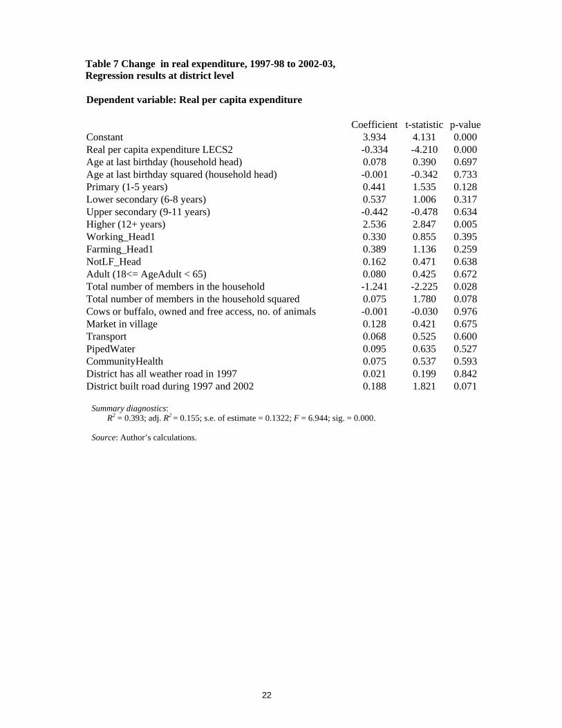
The change in average real expenditures per capita between LECS 2 and LECS 3 was

then related to the improvement or non-improvement of roads as captured in this data set. The

results are summarized in Table 7. The base level of real per capita expenditures in LECS 2

(1997-98) was significant and with a negative coefficient, meaning that better off households

did less well in proportional terms (the dependent variable is the change in the log of real

expenditures) than poorer households. The base level of road access in 1997-98 was less

important in explaining the improvement in average real consumption expenditures at the

district level than the change in road access, where the coefficient was highly significant and

numerically of similar magnitude to the value obtained from the cross sectional results.

A further, more direct, test of the endogenous placement problem was conducted by

regressing the change in road access that occurred between LECS 2 and 3 on the level of

initial real per capita expenditure in LECS 2. The regression was done using regional level

observations by taking the means of the district level dummy variables for improved road

access for each district within the region and regressing this on the regional means of the

district level real per capita expenditure as recorded in LECS 2. If better off areas received

preferential treatment in road improvement a significant and positive coefficient would be

expected. The estimated coefficient was negative but insignificant. These results are

supportive of the findings of the cross-sectional analysis reported above, confirming that

improved road access raises real consumption expenditures and thereby reduces poverty.

4. Conclusions

16

Between 1997-98 and 2002-03, rural poverty incidence in Laos declined by 9.5 per cent of the

rural population. This occurred even though some of the macroeconomic conditions in Laos

mitigated, to some extent, against the interests of rural people. The analysis of the relationship

between poverty incidence and road development provided in this paper suggests that about 13

per cent of this decline in rural poverty can be attributed to improved road access alone.

Between 1997-98 and 2002-03 the improvement in road access took the form of

providing wet weather access to areas which already had dry season access. The analysis

provided in this paper suggests that this strategy had a high pay-off in terms of reduced

poverty incidence. Additional investments in this form of road provision offer the opportunity

for further poverty reduction. Nevertheless, there is now a high return to providing dry

weather access to the most isolated households of Laos – those who have no road access at all.

They constitute 31.6 per cent of all rural households in Laos and are being left behind by the

development of the market economy. By providing them with dry season road access, rural

poverty incidence could be reduced permanently from the present 33 per cent to 29.7 per cent.

A further reduction to 26 per cent could be obtained by providing all rural households with all-

weather road access.

The benefits of rural road provision, measured in terms of poverty reduction or any other

dimension of economic welfare, must of course be compared with its costs. Nevertheless, the

results of this study confirm that in a country like Laos, where roads are primitive, improving

road access is an effective way of reducing rural poverty.

17

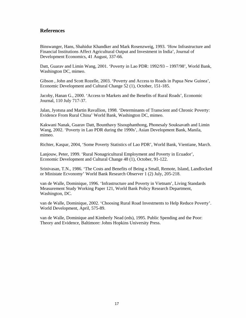
References

Binswanger, Hans, Shahidur Khandker and Mark Rosenzweig, 1993. ‘How Infrastructure and Financial Institutions Affect Agricultural Output and Investment in India’, Journal of Development Economics, 41 August, 337-66.

Datt, Guarav and Limin Wang, 2001. ‘Poverty in Lao PDR: 1992/93 – 1997/98’, World Bank, Washington DC, mimeo.

Gibson , John and Scott Rozelle, 2003. ‘Poverty and Access to Roads in Papua New Guinea’, Economic Development and Cultural Change 52 (1), October, 151-185.

Jacoby, Hanan G., 2000. ‘Access to Markets and the Benefits of Rural Roads’, Economic Journal, 110 July 717-37.

Jalan, Jyotsna and Martin Ravallion, 1998. ‘Determinants of Transcient and Chronic Poverty: Evidence From Rural China’ World Bank, Washington DC, mimeo.

Kakwani Nanak, Guarav Datt, Bounthavy Sisouphanthong, Phonesaly Souksavath and Limin Wang, 2002. ‘Poverty in Lao PDR during the 1990s’, Asian Development Bank, Manila, mimeo.

Richter, Kaspar, 2004, ‘Some Poverty Statistics of Lao PDR’, World Bank, Vientiane, March.

Lanjouw, Peter, 1999. ‘Rural Nonagricultural Employment and Poverty in Ecuador’, Economic Development and Cultural Change 48 (1), October, 91-122.

Srinivasan, T.N., 1986. ‘The Costs and Benefits of Being a Small, Remote, Island, Landlocked or Ministate Ecvonomy’ World Bank Research Observer 1 (2) July, 205-218.

van de Walle, Dominique, 1996. ‘Infrastructure and Poverty in Vietnam’, Living Standards Measurement Study Working Paper 121, World Bank Policy Research Department, Washington, DC.

van de Walle, Dominique, 2002. ‘Choosing Rural Road Investments to Help Reduce Poverty’. World Development, April, 575-89.

van de Walle, Dominique and Kimberly Nead (eds), 1995. Public Spending and the Poor: Theory and Evidence, Baltimore: Johns Hopkins University Press.

18

Table 1 Poverty incidence and inequality in Laos, 1992 to 2002 (Units: per cent, except Gini coefficient)

National

Poverty Rural

Poverty Urban

Poverty Gini

Coefficient 1992-93 46.0 51.8 26.5 0.31 1997-98 39.1 42.5 22.1 0.35 2002-03 30.7 33.0 23.0 0.33

Source: Kaspar Richter, ‘Some Poverty Statistics of Lao PDR’, World Bank, Vientiane, March 2004. Note: 2002-03 estimates are preliminary. Note: National poverty is the percentage of the total population of the country whose real expenditures fall below a poverty line held constant over time in real terms; rural poverty is the percentage of the rural population whose real expenditures fall below a poverty line held constant over time in real terms, and so forth.

Table 2 Laos: Numbers of households by road access, LECS 2 and LECS 3 surveys

Number of households Per cent of households LECS II

1997-98 LECS III 2002-03

LECS II 1997-98

LECS III 2002-03

No access any season

2,146

2,052

31.2

31.6

Dry season access only

1,934

1,050

28.1

16.2

Dry and wet season access

2,794

3,386

40.7

52.2

All households

6,874

6,488

100

100

Source: Author’s calculations from LECS survey data.

19

Table 3 Regression results: LECS 2 (1997-98)

Dependent variable: Log of real per capita expenditure Independent variables: Coefficient t-statistic p-value Constant 11.646 110.094 0.000 Age at last birthday (household head) 0.024 5.755 0.000 Age at last birthday squared (household head) 0.000 -5.015 0.000 Primary (1-5 years) 0.217 9.609 0.000 Lower secondary (6-8 years) 0.306 10.420 0.000 Upper secondary (9-11 years) 0.382 8.844 0.000 Higher (12+ years) 0.476 8.257 0.000 Working head1 0.219 5.239 0.000 Farming head1 -0.155 -4.718 0.000 Head -0.050 -1.490 0.136 Adult (18<= AgeAdult < 65) 0.041 4.612 0.000 Total number of members in the household -0.192 -13.484 0.000 Total number of members in the household squared 0.007 7.319 0.000 Cows or buffalo, owned and free access, no. of animals 0.015 8.233 0.000 Market_n 0.096 2.194 0.028 Transport_n 0.050 2.051 0.040 PipedWater_n 0.107 5.151 0.000 CommunityHealth_n 0.056 2.712 0.007 ReachDry_n 0.003 0.112 0.911 ReachRain_n 0.123 4.835 0.000 Prov. 1 – Phongsaly 0.786 10.145 0.000 Prov. 2 – Luang Namtha -0.115 -2.239 0.025 Prov. 3 – Bokeo -0.087 -1.621 0.105 Prov. 4 – Oudomsay -0.262 -4.866 0.000 Prov. 5 – Sayabouri 0.027 0.528 0.597 Prov. 6 – Luang Prabang 0.181 3.423 0.001 Prov. 7 – Huaphanh -0.262 -5.063 0.000 Prov. 8 – Xieng Khouang 0.563 10.497 0.000 Prov. 9 – Vientiane Municipality 0.136 2.596 0.009 Prov. 10 – Vientiane 0.460 8.211 0.000 Prov. 11 – Saysomboune 0.001 0.019 0.985 Prov. 12 – Borikhamsay -0.146 -2.700 0.007 Prov. 13 – Khammouane 0.070 1.296 0.195 Prov. 14 – Savannakhet 0.141 2.704 0.007 Prov. 15 – Champasack -0.102 -1.885 0.060 Prov. 16 – Saravane 0.184 3.271 0.001 Prov. 17 – Sekong 0.039 0.761 0.446 Summary diagnostics: No. of observations = 6,874. R2 = 0.285; adj. R2 = 0.281; s.e. of estimate = 0.723; F = 75.73; sig. = 0.000.

Source: Author’s calculations from LECS 2 survey data.

20

Table 4 Regression results: LECS 3 (2002-03)

Dependent variable: Log of real per capita expenditure Independent variables: Coefficient t-statistic p-value(Constant) 10.911 87.710 0.000 Age at last birthday 0.032 7.073 0.000 Age at last birthday squared (household head) 0.000 -6.138 0.000 Primary (1-5 years) 0.140 6.159 0.000 Lower secondary (6-8 years) 0.330 10.439 0.000 Upper secondary (9-11 years) 0.380 6.900 0.000 Higher (vocational training or university/institute) 0.541 9.679 0.000 Paid employment 0.257 4.623 0.000 Farm employment 0.055 1.021 0.307 Not in labor force 0.135 2.098 0.036 Number of adults in household (18 <= AgeAdult < 65) 0.060 6.070 0.000 Total number of members in household -0.115 -23.015 0.000 Total number of cows and buffaloes 0.021 11.543 0.000 Electricity 0.194 8.408 0.000 DailyMarket 0.084 1.381 0.167 BusStop 0.029 0.988 0.323 CleanWater 0.061 2.883 0.004 Hospital inVillage 0.350 5.619 0.000 Access Dry Season 0.102 3.403 0.001 Access Wet Season 0.086 2.638 0.008 Prov. 1 – Phongsaly 0.206 2.473 0.013 Prov. 2 – Luang Namtha -0.354 -4.705 0.000 Prov. 3 – Bokeo 0.020 0.277 0.782 Prov. 4 – Oudomsay -0.076 -1.010 0.312 Prov. 5 – Sayabouri -0.060 -0.813 0.416 Prov. 6 – Luang Prabang 0.245 3.499 0.000 Prov. 7 – Huaphanh 0.006 0.089 0.929 Prov. 8 – Xieng Khouang 0.533 7.775 0.000 Prov. 9 – Vientiane Municipality 0.063 0.832 0.405 Prov. 10 – Vientiane 0.315 4.534 0.000 Prov. 11 – Saysomboune 0.126 1.724 0.085 Prov. 12 – Borikhamsay 0.040 0.567 0.571 Prov. 13 – Khammouane -0.028 -0.413 0.680 Prov. 14 – Savannakhet -0.269 -3.925 0.000 Prov. 15 – Champasack -0.380 -4.776 0.000 Prov. 16 – Saravane 0.145 2.115 0.034 Prov. 17 – Sekong -0.380 -5.007 0.000 Summary diagnostics: No. of observations = 6,488. R2 = 0.318; adj. R2 = 0.314; s.e. of estimate = 0.729; F = 85.55; sig. = 0.000.

Source: Author’s calculations from LECS 3 survey data.

21

Table 5 Estimated poverty incidence (%) under alternative road conditions –

LECS 2 – 1997-98

Dry season road access

Wet season road access

Code Estimated poverty

incidence (%)

Observed levels in data

Observed levels in data

P1 42.50

All households with access Observed levels in data

P2 42.44

All households with access All households with

access

P3 34.86

Source: Author’s calculations.

Table 6 Estimated poverty incidence (%) under alternative road conditions –

LECS 3 – 2002-03

Dry season road access

Wet season road access

Code Estimated poverty

incidence (%)

Observed levels in data

Observed levels in data

P1 33.00

All households with access Observed levels in data

P2 29.68

All households with access All households with

access

P3 25.91

Source: Author’s calculations.

22

Table 7 Change in real expenditure, 1997-98 to 2002-03, Regression results at district level Dependent variable: Real per capita expenditure Coefficient t-statistic p-valueConstant 3.934 4.131 0.000 Real per capita expenditure LECS2 -0.334 -4.210 0.000 Age at last birthday (household head) 0.078 0.390 0.697 Age at last birthday squared (household head) -0.001 -0.342 0.733 Primary (1-5 years) 0.441 1.535 0.128 Lower secondary (6-8 years) 0.537 1.006 0.317 Upper secondary (9-11 years) -0.442 -0.478 0.634 Higher (12+ years) 2.536 2.847 0.005 Working_Head1 0.330 0.855 0.395 Farming_Head1 0.389 1.136 0.259 NotLF_Head 0.162 0.471 0.638 Adult (18<= AgeAdult < 65) 0.080 0.425 0.672 Total number of members in the household -1.241 -2.225 0.028 Total number of members in the household squared 0.075 1.780 0.078 Cows or buffalo, owned and free access, no. of animals -0.001 -0.030 0.976 Market in village 0.128 0.421 0.675 Transport 0.068 0.525 0.600 PipedWater 0.095 0.635 0.527 CommunityHealth 0.075 0.537 0.593 District has all weather road in 1997 0.021 0.199 0.842 District built road during 1997 and 2002 0.188 1.821 0.071

Summary diagnostics:

R2 = 0.393; adj. R2 = 0.155; s.e. of estimate = 0.1322; F = 6.944; sig. = 0.000.

Source: Author’s calculations.

23

Figure 1 Laos: Real GDP growth (%) and CPI inflation (%)

Source: Author’s calculations using data from National Statistical Centre, Vientiane. Note: GDP growth is deflated by the GDP deflator.

4.0

6.5

8.1

4.0

5.55.75.75.8

7.36.96.97.06.6

13.027.5 27.1

11.410.67.86.87.08.010.419.6

134.0

87.4

0123456789

1991 1992 1993 1994 1995 1996 1997 1998 1999 2000 2001 2002 2003

GDP Growth

0

20

40

60

80

100

120

140

160CPI

GDP (% - Left axis) CPI (% - Right axis)

24

Figure 2 Laos: Relative prices, food to non-food, 1988 to 2004

0.0

0.2

0.4

0.6

0.8

1.0

1.2

1.4

1988 1989 1990 1991 1992 1993 1994 1995 1996 1997 1998 1999 2000 2001 2002 2003 2004

Rel

ativ

e Pr

ices

Relative prices: Food / Services

Source: Author’s calculations using data from National Statistical Centre, Vientiane.

25

Figure 3 Predicted distribution of real expenditures per person under alternative road conditions: LECS 2 – 1997-98

Source: Author’s calculations based on LECS 2 household survey data from National Statistical Center, Vientiane, and regression results shown in Table 3, above. Note: Units on the horizontal axis are the natural logarithm of real household consumption expenditures per person expressed in December 1999 prices. “real per capita exp. (predicted)” refers to P1 in the text. “real per capita exp. (predicted all dry)” refers to P2 in the text. “real per capita exp. (predicted)” refers to P3 in the text.

0%

10%20%

30%

40%

50%60%

70%

80%90%

100%

10.50 11.00 11.50 12.00 12.50 13.00 13.50 14.00

real expenditure per person (natural logarithm)

per c

ent o

f rur

al p

opul

atio

n

real per capita exp. (predicted)

real per capita exp. (predicted all dry)

real per capita exp. (predicted all wet)

26

Figure 4 Predicted distribution of real expenditures per person under alternative road conditions: LECS 3 – 2002-03

Source: Author’s calculations based on LECS 3 household survey data from National Statistical Center, Vientiane, and regression results shown in Table 4, above. Note: Units on the horizontal axis are the natural logarithm of real household consumption expenditures per person expressed in December 1999 prices. “real per capita exp. (predicted)” refers to P1 in the text. “real per capita exp. (predicted all dry)” refers to P2 in the text. “real per capita exp. (predicted)” refers to P3 in the text.

0%

10%

20%

30%

40%

50%

60%

70%

80%

90%

100%

9.50 10.50 11.50 12.50 13.50 14.50

real expenditure per person (natural logarithm)

per c

ent o

f rur

al p

opul

atio

n

real per capita exp. (predicted)

real per capita exp. (predicted all dry)

real per capita exp. (predicted all wet)