NASA Technical Memorandum 107318

RL10A-3-3A Rocket Engine

Modeling Project

Michael Binder

NYMA, Inc.

Brook Park, Ohio

Thomas Tomsik and Joseph P. Veres

Lewis Research Center

Cleveland, Ohio

January 1997

NationalAeronauticsandSpace Administration

https://ntrs.nasa.gov/search.jsp?R=19970010379 2018-06-01T06:14:54+00:00Z

°

2.

TABLE OF CONTENTS

Page

Introduction ............................................................................................................................................... 1

Overview of the RL10A-3-3A Rocket Engine ............................................................................................ 2

2.1 Engine System Configuration and Operation ....................................................................... 22.2 Fuel Turbopump ..................................................................................................... 4

2.3 Oxygen (LOX) Pump ...................................................................................................................... 5

2.4 Regenerative Cooling Jacket ....................................................................................................... 52.5 Combustion Chamber and Nozzle ......................................................................................... 6

2.6 Valves, Ducts and Manifolds ............................................................................................................. 6

3. Project Organization and Goals ........................................................................................................................... 7

3.1 Turbomachinery Modeling Goals .................................................................................................... 73.2 Combustion and Heat Transfer Modeling Goals .......................................................... 8

3.3 Ducts, Manifolds, and Valves Modeling Goals ........................................................................ 8

3A System Modeling Goals .......................................................................................................... 8

4. Component Modeling Results ............................................................................................................................. 9

4.1 Turbomachinery Modeling Results ................................................................................................... 94.1.1 Verification of Pump Performance Test Data ............................................................. 9

4.1.2 Extension of Pump Maps for Start and Shutdown Conditions ................................... 94.1.2.1 Extension of Pump Maps to Start Conditions ............................................. 10

4.1.2.2 Extension of Pump Maps to Shut-Down Conditions .............................. 114.1.2.3 Effects of Density Changes on Pump Performance Models ................... 11

4.1.3 Verification of Fuel Turbine Performance Test Data .................................................. 12

4.1.4 Extension of Turbine Maps ........................................................................................ 12

4.2 Combustion and Heat Transfer Modeling Results ......................................................................... 13

4.2.1 Enhanced Combustion Gas Properties ........................................................................... 13

4.2.2 Cooling Jacket Heat Transfer Model ................................................................................... 134.2.3 Thrust Chamber Performance Calculations ........................................................................... 15

4.2_3.1 One-dimensional combustion model layout ....................................................... 15

4.2.3.2 Detailed modeling of the chamber injector ........................................................ 16

4.2.3.3 Nozzle performance models ........................................................................ 16

4.2.3.4 Two-phase flow through nozzle ........................................................... 17

4.2.4 Injector Heat-Transfer Calculations .................................................................... 17

4.3 Duct,4.3.1

4.3.2

4.3.3

4.3.44.3.5

Valve, and Manifold Modeling Results ............................................................ 18

Verification of Duct, Manifold Sizes ............................................................................. 18

Prediction of Fluid Frictional Resistances ...................................................................... 18

Modeling of Valve Actuator Mechanisms .................................................................... 19Modeling of Critical Two-Phase Flow Through a Valve or Orifice ................................ 19

Model of Flow Through Venturi .............................................................................. 21

4.4 The New RL10A-3-3A System Model ............................................................................................ 22

4.4.1 Evaluation of Component Models/Integration With New System Model ....................... 21

4.4.2 Differences Between Start and Shutdown System Models .................................................. 22

5. ModelingUncertainties ..................................................................................... 22

5.1 Hardware Uncertainties .................................................................. .23

5.2 Valve Uncertainties .............................................................................................. 23

5.3 Uncertainty of Initial Conditions .......................................................................... 24

5.4 Uncertainty in Ignition Time ....................................................................................... 245.5 Interaction Between Uncertain Parameters ........................................................................... 25

6. Comparison of System Model Predictions With Test Data .................................................................... 25

6.1 Verification of Steady State Performance Predictions .................... 256-2 Verification for Start Transient Simulations .......................................................... 26

6.3 Verification of Shutdown Transient Simulations ....... 27

7. Discussion of Modeling Results ............................................................................................27

7.1 Discussion of Turbomachinery Investigation ................................................................................... 27

7-2 Discussion of Combustion and Heat Transfer Investigation ................................................ 287.3 Discussion of Duct, Manifold and Valve Investigation .................................................................. 29

7.4 Discussion of System Model Simulation Results .................................................................................. 29

8. Concluding Remarks .............................................................................................................................................. 29

9. Recommendations for Future Research ........................................................................................ 31

10. Def'mition of Terms ............................................................................................................. 33

11. Acknowledgments .......................................................................................................................... 34

12. AppendixesA RL10A-3-3A Engine System Model for ROCETS .................................................................................... 87

B----Component Modeling of RL10 Fuel and Oxidizer Pumps ............................................................... 89

C---Component Modeling of RL10 Fuel Turbine .................................................................... 109

D---Component Modeling of RL 10A-3-3A Cooling Jacket ................................................ 119

E---Component Modeling of RL10 Injector, Combustion Chamber, and Nozzle ................... 135

F---Component Modeling of RL10 Injector Heat Transfer ............................................................... 149

G---Component Modeling of RL10 Duct Flow ..................................................................... 157

H Modeling of Two-Phase (Liquid/Gas) Flow ................................................................... 163

I---Symbols ......................................................................................................................... 171J--Glossary of Model Component Names ................................................................................................. 173

13. References ................................................................................................................................................... 175

14. Tables

2.2.1--Summary of Fuel Turbopump Characteristics .............................................................................. 42.3.1---Summary of LOX Pump Characteristics ............................................................................................ 52.4.1mSummary of Cooling Jacket Characteristics ............................................................................... 52.5.1--Summary of Combustion Chamber/Nozzle Characteristics ................................................ 62.6.1--Summary of Major Duct and Valve Characteristics ................................................................ 74-2.1mDescription of Combustion Property Tables for RL10 Model ...................................................... 354.3.I----Comparison of Model Dynamic Volume Sizes ...................................................................... 366.1.1--Steady-State Cycle Performance Prediction for the RL10A-3-3A ........................................................ 376-2.1--Comparison of Measured and Predicted RL10 Engine Time-to-Accelerate ................................... 38

ii

15.Figures2.1.1--RL10A-3-3A Engine System Schematic ......................................................................... 392.1.2_R.L10 Assumed Valve Schedules for Start Simulation ......................................................... 402.1.3--RL10 Assumed Valve Schedules for Shutdown Simulation .............................................. 412.2.I----Cross-section of Fuel Pump and Turbine ....................................................................................... 422.3.1---Cross Section of LOX Pump and GearBox ......................................................................... 432.4.1---Structure of Regenerative Cooling Jacket, Chamber and Nozzle .................................. 44

2.5. I--Injector Design Configuration ....................................................................................... 454.1.1---Original Head Map for Fuel Pump 1st Stage (provided by P&W) ............................. .464.1.2----Original Head Map for Fuel Pump 2nd Stage (provided by P&W) _._.464.1.3--Original Efficiency Map for Fuel Pump 1st stage (provided by P&W ..... .474.1.4----Original Efficiency Map for Fuel Pump 2nd stage (provided by P&W__ _.474.1.5---Efficiency Speed Correction Map for Fuel Pump - both stages (,provided by P&W) ........... 484.1.6--Original Head Map for LOX Pump (provided by P&W) ............................................... _484.1.7---Original Efficiency Map for LOX Putnp (provided by P&W) ............................................ .494.1.8--Efficiency Speed Correction Map for LOX Pump (provided by P&W) .......................... 494.1.9----Generic Wide-Range Performance Maps for Centrifugal and Mixed-Flow Pumps ............... 504.1.10---Extended Head Map for Fuel Pump 1st Stage ........................................................... 514.1.11--Extended Torque Map (w/o Speed Correction) for Fuel Pump 1st Stage .... 514.1.12--Extended Head Map for Fuel Pump 2nd Stage ...................................................... 524.1.13---Extended Torque Map (w/o Speed Correction) for Fuel Pump 2nd Stage ........................... 524.1.14--Extended Head Map for LOX Pump ...................................................................................... 534.1.15--Extended Torque Map (w/o Speed Correction) for LOX Pump ..................................... 534.1.16--Fuel Turbine Effective Flow Area Map (provided by P&W and Martin-Marietta) ........... 544.1.17--Fuel Turbine Efficiency Map (provided by P&W and Martin-Marietta) ........................ 54

4.2.1---Configuration of Cooling Jacket and Model ........................................................................ 554_2.2---Comparison of Full 20-Node Model with 20-Metal-Nod_5-Fluid-Node Model .................. 564.2.3----Comparison of Enthalpy-Driven and Temperature-Driven Potential Predictions ................ 574.2.4---Predicted Heat Flux Distribution ............................................................................................ 574.2.5---Predicted Hot-Wall Metal Temperature Distribution ...................................................................... 584.2.6--Predicted Coolant Temperature Distribution ............................................................................ 584.2.7--Predicted Coolant Pressure Distribution ....................................................................... 594.2.8---c*-Efficiency Maps (from P&W) ................................................................................... 594.2.9--TDK/ODE Predictions of RL10A-3-3A Actual Isp, compared to data provided by P&W ..... 604.2.10---TDK Predictions of RL10A-3-3A Thrust-Coefficient Efficiency ...................................... 60

4.2.11--Injector Heat Transfer Model Configuration ............................................................ 614.2.12--Injector Heat Transfer Rate during start sequence_. __.614.3. I--Predicted Mass Flux for Choked Two-phase Flow .... ._.624.3.2--RL10 Venturi Flow Parameter Map ...................................................................................... 62

4.4.1--RL10A-3-3A Engine System Model Schematic ........................................................... .635.1.1--Variation in Start with Cooldown Valve Effective Area ........................................................... 645.1.2--Variation in Start with Turbopump Drag Torque ................................................................. 655.2.1--Variation in Start with OCV Actuation Pressure ............................................................ 665.2.2---OCV Position during Start as Estimated from Test Data. ........................................................ 675.3.1--Variation in Start with Initial Jacket Metal Temperature ................................................ 685.4.1--Variation in Start with Assumed Ignition Time-delay ................................................ 696.1.1--Steady-State Predictions vs. Measured Values (error distribution) .................................... 706.2.1--MES 1 Chamber Pressure - Simulation vs. Ground-Test Data. ................................... .70

6_2.2 MES1 LOX Pump Shaft Speed - Simulation vs. Ground-Test Data ............................... 716.2.3--MES1 Fuel Venturi Inlet Pressure - Simulation vs. Ground-Test Data ...... 71

6.2.4--MES1 LOX Pump Discharge Pressure - Simulation vs. Ground-Test Data. ..................... 726.2.5--MES1 Turbine Inlet Temperature - Simulation vs. Ground-Test Data ................................. 726.2.6---MES1 LOX Pump Inlet Pressure - Simulation vs. Ground-Test Data .................................... 73

6.2.7--MES1 Engine Fuel Inlet Flow - Simulation vs. Ground-Test Data ......................................... 736.2.8--MES 1 Engine LOX Inlet Flow - Simulation vs. Ground-Test Data. .......................................... 746.2.9--MES2 Chamber Pressure during Start - Simulation vs. Ground-Test Data. ............................. 746.2.10---MES1 Chamber Pressure - Simulation vs. Centaur Flight Data ................................................. 756_..ll--MES1 LOX Pump Shaft Speed - Simulation vs. Centaur Flight Data ........................................... 756.2.12_MES1 Turbine Inlet Temperature - Simulation vs. Centaur Flight Data .................................... 76

.°.

111

Figures--Continued6_.13--MES2 Chamber Pressure - Simulation vs. Centaur Flight Data ................. 766.2.14---Predicted Maximum Metal Temperature during Start Transient .................... 776.2.15--Predicted Ignitor GOX Supply delta-P during Start (variation with OCV opening pressure)__776.3.1--MECO1 Chamber Pressure - Simulation vs. Ground-Test Data. ......... 78

6.3.2 MECO1 LOX Pump Shaft Speed - Simulation vs. Ground-Test Data ............ 786.3.3---MECO1 Fuel Venturi Inlet Pressure - Simulation vs. Ground-Test Data ......................... 79

6.3.4--MECO1 LOX Pump Discharge Pressure - Simulation vs. Ground-Test Data. ....................... 796.3.5--MECO1 Fuel Pump Inlet Pressure - Simulation vs. Ground-Test Data. ......................... 806.3.6--MECO1 LOX Pump Inlet Pressure - Simulation vs. Ground-Test Data .............. 806.3.7--MECO1 Engine Inlet LOX Flow - Simulation vs. Ground-Test Data.. ........................ 816.3.8---MECO1 Engine Inlet Fuel Flow - Simulation vs. Ground-Test Data ........................ 816.3.9mMECO1 Chamber Pressure - Simulation vs. Centaur Flight Data. ........................ 826.3.10--MECO1 LOX Pump Shaft Speed - Simulation vs. Centaur Flight Data.. ................ 826.3.11--MECO1 Fuel Venturi Inlet Pressure - Simulation vs. Centaur Flight Data. .................. 836.3.12--MECO1 LOX Pump Discharge Pressure - Simulation vs. Centaur Flight Data ................. 836.3.13--MECO1 Fuel Pump Inlet Pressure - Simulation vs. Centaur Flight Data ......................... 846.3.14---MECO1 LOX Pump Inlet Pressure - Simulation vs. Centaur Flight Data_ ................... 846.3.15---Range of Predicted Shutdown Profiles (Ground Test Conditions) ............................ 856.3.16---Range of Measured Shutdown Profiles (Ground Test Data) ...................................................... 85

iv

1. INTRODUCTION

The RL10A rocket engine is an important component of the American space infrastructure. Two

RL10 engines form the main propulsion system for the Centaur upper stage vehicle, which boostscommercial, scientific, and military payloads from a high altitude into Earth orbit and beyond

(planetary missions). The Centaur upper stage is used on both Atlas and Titan launch vehicles.The initial RL10A-1 was developed in the 1960's by Pratt & Whitney, under contract to NASA.

The RL10A-3-3A, RL10A-4, and RL10A4-1 engines used today incorporate component

improvements but have the same basic configuration as that of the original RL10A-1 engine.RL10's have been highly reliable servants of America's space program for over 30 years.

The RL10's high reliability record has been marred in recent years by two in-flight failures. In thefirst instance, the cause was initially believed to be Foreign Object Damage of the fuel pump. In

the second instance, the cause of failure was determined to be contamination of the fuel pump by

atmospheric nitrogen which leaked through a check valve during Munch ascent. The nitrogen froze

on the impeller and prevented pump rotation during start. In hindsight, it is likely that the firstfailure was also due to frozen atmospheric nitrogen. During the course of the accident

investigations, the desire for an independent RL10 simulation capability was expressed within

NASA and by the Air Force. At that time, the only system models for the engine were the

property of Pratt & Whitney and of the Aerospace Corporation. These models are not suitable for

public dissemination or government use. The Space Propulsion Technology Division (SPTD) atthe NASA Lewis Research Center took up the challenge of creating an independent and accurate

model of the RL10A-3-3A engine.

The SPTD began developing a computer model of the RL10A-3-3A in 1990 (Reference 1). The

first system model was based entirely on data and information provided by Pratt &Whitney.

Component data f_om Pratt & Whitney was integrated to form a system model using the ROcket

Engine Transient Simulator (ROCETS) code. In 1993, a project team was formed, consisting of

experts in the areas of turbomachinery, combustion, and heat transfer. The goals of this projecthave been to enhance our understanding of the RL10 engine and its components, and to improve

the baseline engine system model where possible. A combination of simple engineeringcorrelations, detailed component analyses and engineering judgement have been used to

accomplish these tasks. If desired, it should be a relatively simple task to create models of theRL10A-4 and RL10A4-1 as well, using the work done here for the RL10A-3-3A as a foundation.

A second goal of this project was to benchmark our tools and methods for modeling new rocket

engine components and systems, for which test data may not yet be available. An existing enginewith a long test and flight history (the RL10A-3-3A) was used as the validation test-case.

In this report, we introduce the reader to the RL10 engine, define the SPTD project organization

and goals, briefly discuss results of the various component modeling efforts, and describe the new

RL10 system model created. The appendices contain detailed descriptions of the various

component analyses performed in support of the project.

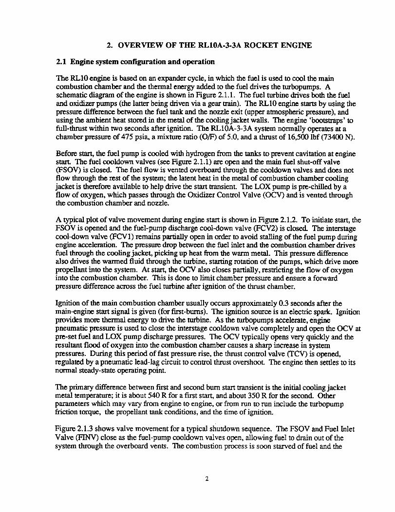
2. OVERVIEW OF THE RL10A-3-3A ROCKET ENGINE

2.1 Engine system configuration and operation

The RL10 engine is based on an expander cycle, in which the fuel is used to cool the main

combustion chamber and the thermal energy added to the fuel drives the turbopumps. Aschematic diagram of the engine is shown in Figure 2.1.1. The fuel turbine drives both the fuel

and oxidizer pumps (the latter being driven via a gear train). The RL10 engine starts by using thepressure difference between the fuel tank and the nozzle exit (upper atmospheric pressure), and

using the ambient heat stored in the metal of the cooling jacket walls. The engine 'bootstraps' tofull-thrust within two seconds after ignition. The RL10A-3-3A system normally operates at a

chamber pressure of 475 psia, a mixture ratio (O/F) of 5.0, and a thrust of 16,500 lbf (73400 N).

Before start, the fuel pump is cooled with hydrogen from the tanks to prevent cavitation at engine

start. The fuel cooldown valves (see Figure 2.1.1) are open and the main fuel shut-off valve(FSOV) is closed. The fuel flow is vented overboard through the cooldown valves and does not

flow through the rest of the system; the latent heat in the metal of combustion chamber cooling

jacket is therefore available to help drive the start transient. The LOX pump is pre-chilled by a

flow of oxygen, which passes through the Oxidizer Control Valve (OCV) and is vented throughthe combustion chamber and nozzle.

A typical plot of valve movement during engine start is shown in Figure 2.1.2. To initiate start, the

FSOV is opened and the fuel-pump discharge cool-down valve (FCV2) is closed. The interstage

cool-down valve (FCV 1) remains partially open in order to avoid stalling of the fuel pump duringengine acceleration. The pressure drop between the fuel inlet and the combustion chamber drives

fuel through the cooling jacket, picking up heat from the warm metal. This pressure difference

also drives the warmed fluid through the turbine, starting rotation of the pumps, which drive more

propellant into the system. At start, the OCV also closes partially, restricting the flow of oxygeninto the combustion chamber. This is done to limit chamber pressure and ensure a forward

pressure difference across the fuel turbine after ignition of the thrust chamber.

Ignition of the main combustion chamber usually occurs approximately 0.3 seconds after the

main-engine start signal is given (for first-burns). The ignition source is an electric spark. Ignition

provides more thermal energy to drive the turbine. As the turbopumps accelerate, engine

pneumatic pressure is used to close the interstage cooldown valve completely and open the OCV at

pre-set fuel and LOX pump discharge pressures. The OCV typically opens very quickly and theresultant flood of oxygen into the combustion chamber causes a sharp increase in system

pressures. During this period of fast pressure rise, the thrust control valve (TCV) is opened,regulated by a pneumatic lead-lag circuit to control thrust overshoot. The engine then settles to its

normal steady-state operating point.

The primary difference between first and second burn start transient is the initial cooling jacketmetal temperature; it is about 540 R for a first start, and about 350 R for the second. Other

parameters which may vary from engine to engine, or from run to run include the turbopump

friction torque, the propellant tank conditions, and the time of ignition.

Figure 2.1.3 shows valve movement for a typical shutdown sequence. The FSOV and Fuel Inlet

Valve (FINV) close as the fuel-pump cooldown valves open, allowing fuel to drain out of the

system through the overboard vents. The combustion process is soon starved of fuel and the

flame goes out. The OCV and Oxidizer Inlet Valve (OINV) begin to close next, cutting off theflow of oxygen through the engine. The turbopump decelerates due to friction losses and dragtorque created by the pumps as they evacuate the remaining propellants from the system. Du_dngthis process, pump cavitation and reverse-flow are likely.

The symbols and model component names used herein are found in appendixes I and J.

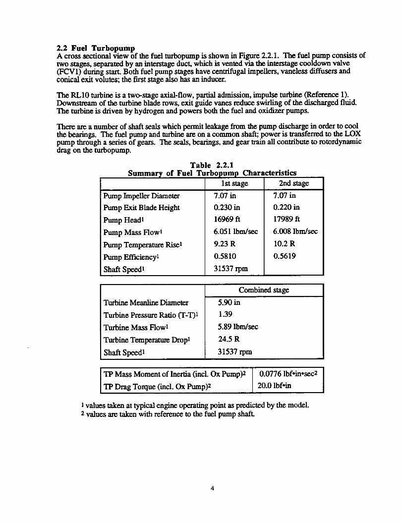
2.2 Fuel TurbopumpA cross sectional view of the fuel turbopump is shown in Figure 2.2.1. The fuel pump consists oftwo stages, separated by an interstage duct, which is vented via the interstage cooldown valve(FCV1) during start. Both fuel pump stages have centrifugal impellers, vaneless diffusers andconical exit volutes; the first stage also has an inducer.

The RL10 turbine is a two-stage axial-flow, partial admission, impulse turbine (Reference 1).Downstream of the turbine blade rows, exit guide vanes reduce swirling of the discharged fluid.

The turbine is driven by hydrogen and powers both the fuel and oxidizer pumps.

There are a number of shaft seals which permit leakage from the pump discharge in order to coolthe bearings. The fuel pump and turbine are on a common shaft; power is transferred to the LOXpump through a series of gears. The seals, bearings, and gear train all contribute to rotordynamicdrag on the turbopump.

Table 2.2.1

Summary of Fuel Turbopump Characteristics

1st stage 2nd stage

Pump Impeller Diameter

Pump Exit Blade Height

Pump Headl

Pump Mass Howl

Pump Temperature Risel

Pump Efficiencyt

Shaft Speedl

7.07 in

0.230 in

16969 ft

6.051 Ibm/see

9.23 R

0.5810

31537 rpm

7.07 in

0.220 in

17989 ft

6.008 lbm/sec

10.2 R

0.5619

Turbine Meanline Diameter

Turbine Pressure Ratio (T-T)1

Turbine Mass Flow1

Turbine Temperature Dropl

Shaft Speedl

Combined stage

5.90 in

1.39

5.89 Ibm/see

24.5 R

31537 rpm

TP Mass Moment of Inertia (incl. Ox Pump)2TP Drag Torque (incl. Ox Pump)2

0.0776 lbf.in.sec2

20.0 lbf-in

I values taken at typical engine operating point as predicted by the model.

2 values are taken with reference to the fuel pump shaft.

4

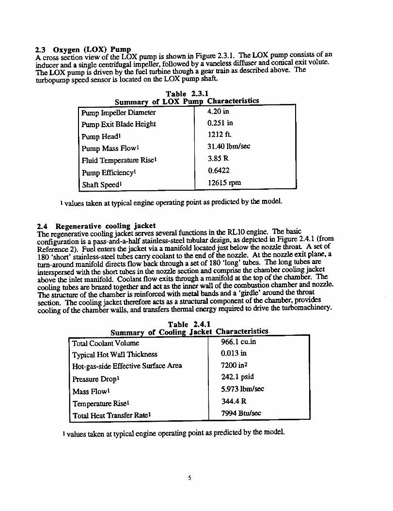
2.3 Oxygen (LOX) PumpA cross section view of the LOX pump is shown in Figure 2.3.1. The LOX pump consists of an

inducer and a single centrifugal impeller, followed by a vaneless diffuser and conical exit volute.The LOX pump is driven by the fuel turbine though a gear train as described above. Theturbopump speed sensor is located on the LOX pump shaft.

Table 2.3.1

Summary of LOX Pump Characteristics

Pump Impeller Diameter

Pump Exit Blade Height

Pump Headl

Pump Mass Flow1

Fluid Temperature Rise1

Pump Efficiencyl

Shaft Speed1

4.20 in

0.251 in

1212 ft.

31.40 lbm/sec

3.85 R

0.6422

12615 rpm

1 values taken at typical engine operating point as predicted by the model.

2.4 Regenerative cooling jacketThe regenerative cooling jacket serves several functions in the RL10 engine. The basicconfiguration is a pass-and-a-half stainless-steel tubular design, as depicted in Figure 2.4.1 (fromReference 2). Fuel enters the jacket via a manifold located just below the nozzle throat. A set of180 'short' stainless-steel tubes carry coolant to the end of the nozzle. At the nozzle exit plane, aturn-around manifold directs flow back through a set of 180 'long' tubes. The long tubes are

interspersed with the short tubes in the nozzle section and comprise the chamber cooling jacketabove the inlet manifold. Coolant flow exits through a manifold at the to.p of the chamber. The

cooling tubes are brazed together and act as the inner wall of the combustton chamber and nozzle.The structure of the chamber is reinforced with metal bands and a'girdle' around the throat

section. The cooling jacket therefore acts as a structural component of the chamber, providescooling of the chamber walls, and transfers thermal energy required to drive the turbomachinery.

Table 2.4.1

Summary of Cooling Jacket Characteristics

Total Coolant Volume

Typical Hot Wall Thickness

Hot-gas-side Effective Surface Area

Pressure Dropl

Mass Flow1

Temperature Riser

Total Heat Transfer Rate1

966.1 cu.in

0.013 in

7200 in2

242.1 psid

5.973 Ibm/see

344.4 R

7994 Btu/sec

t values taken at typical engine operating point as predicted by the model.

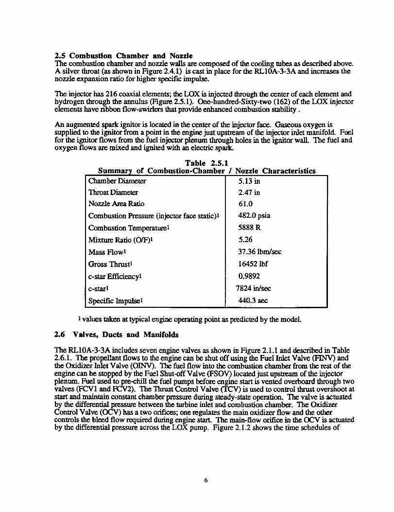
2.5 Combustion Chamber and NozzleThecombustionchamberandnozzlewallsarecomposed of the cooling tubes as described above.A silver throat (as shown in Figure 2.4.1) is cast in place for the RL10A-3-3A and increases thenozzle expansion ratio for higher specific impulse.

The injector has 216 coaxial elements; the LOX is injected through the center of each clement andhydrogen through the annulus (Figure 2.5.1). One-hundred-Sixty-two (162) of the LOX injectorelements have ribbon flow-swirlcrs that provide enhanced combustion stability.

An augmented spark ignitor is located in the center of the injector face. Gaseous oxygen issupplied to the ignitor from a point in the engine just upstream of the injector inlet manifold Fuelfor the ignitor flows from the fuel injector plenum through holes in the ignitor wall. The fuel andoxygen flows axe mixed and ignited with an electric spark.

Table 2.5.1

Summary of Combustion-Chamber / Nozzle CharacteristicsChamber Diameter

Throat Diameter

Nozzle Area Ratio

Combustion Pressure (injector face static)l

Combustion Temperature1

Mixture Ratio(O/F)I

Mass Flowl

Gross Thrustl

c-starEfficicncyl

c-starl

SpecificImpulsel

5.13 in

2.47 in

61.0

482.0 psia

5888 R

5.26

37.36 Ibm/see

16452 lbf

0.9892

7824 in/sec

440.3 sec

1 values taken at typical engine operating point as predicted by the model

2.6 Valves, Ducts and Manifolds

The RL10A-3-3A includes seven engine valves as shown in Figure 2.1.1 and described in Table2.6.1. The propellant flows to the engine can be shut off using the Fuel Inlet Valve (FINV) andthe Oxidizer Inlet Valve (OINV). The fuel flow into the combustion chamber from the rest of theengine can be stopped by the Fuel Shut-off Valve (FSOV) located just upstream of the injectorplenum. Fuel used to pre-ehill the fuel pumps before engine start is vented overboard through twovalves (FCV1 and FCV2). The Thrust Control Valve (TCV) is used to control thrust overshoot atstart and maintain constant chamber pressure during steady-state operation. The valve is actuatedby the differential pressure between the turbine inlet and combustion chamber. The OxidizerControl Valve (OCV) has a two orifices; one regulates the main oxidizer flow and the othercontrols the bleed flow required during engine start. The main-flow orifice in the OCV is actuatedby the differential pressure across the LOX pump. Figure 2.1.2 shows the time schedules of

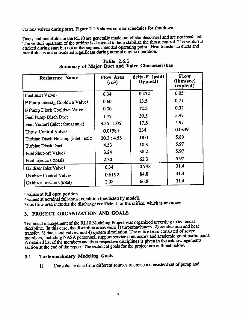
variousvalves during start, Figure 2.1.3 shows similar schedules for shutdown.

Ducts and manifolds in the RL10 are generally made out of stainless-steel and are not insulate&

The venturi upstream of the turbine is designed to help stab'dize the thrust control. The venturi ischoked during start but not at the engines intended operating point. Heat transfer in ducts andmanifolds is not considered significant during normal engine operation.

Table 2.6.1

Summary of Major Duct and Valve Characteristics

Resistence Name

Fuel Inlet Valve1

F Pump Interstg Cooldwn Valve1

iF Pump Disch Cooldwn Valvet

Fuel Pump Disch Duct

Fuel Venturi (inlet : throat area)

Flow Area

(in2)

6.34

0.60

0.30

1.77

3.55 : 1.05

delta-P (psid)

(typical)

0.472

13.5

12.5

39.5

17.5

Thrust Control Valve2

Turbine Disch Housing (inlet : exit)

Turbine Disch Duct

Fuel Shut-off Valve1

Fuel Injectors (total)

OxidizerInletValvel

OxidizerControlValve2

OxidizerInjectors(total)

0.0158 3

20.2 : 4.53

4.53

3.24

2.30

6.34

0.615 3

2.08

234

18.0

10.3

38.2

62.3

0.798

84.8

66.8

Flow

(Ibm/see)(typical)

6._

0.71

0.32

5.97

5.97

0.0839

5.89

5.97

5.97

5._

31.4

31.4

31.4

1 values at full open position2 values at nominal full-thrust condition (predicted by model).

3 this flow area includes the discharge coefficient for the orifice, which is unknown.

3. PROJECT ORGANIZATION AND GOALS

Technical management of the RL10 Modeling Project was organized according to technicaldiscipline. In this case, the discipline areas were 1) turbomachinery, 2) combustion and beattransfer, 3) ducts and valves, and 4) system simulation. The entire team consisted of sevenmembers, including NASA personnel, support service contractors and academic grant participants.A detailed list of the members and their respective disciplines is given in the acknowlegements

section at the end of the report. The technical goals for the project are outlined below.

3.1 Turbomachinery Modeling Goals

1) Consolidate data from different sources to create a consistent set of pump and

3.2

3.3 Ducts,

3.4

turbine performance characteristics for normal operating conditions.

2) Extend the pump and turbine performance maps to include engine start andshutdown transient conditions.

3) Benchmark our analytic capabilities for pumps and turbines over a wider range ofoperating conditions (using available RL10 test data).

Combustion and Heat Transfer Modefing Goals

1) Develop a computer model of heat transfer in the thrust chamber cooling jacket.

2) Develop a one-dimensional model of combustion in the thrust chamber and of hotgas flow through the nozzle.

3) Develop improved hydrogen-oxygen combustion property tables to replace thetables delivered with the ROCETS program.

4) Extend existing data tables of combustion and nozzle performance (c*-efficiencyand specific impulse) to better cover start and shut-down transient conditions.

5) Develop a model of two-phase flow through the nozzle throat.

6) Develop a model of the fuel-to-oxidizer heat transfer in the injector plenum.

7) Benchmark our analytic capabilities for thrust chamber injectors, nozzles, andcooling jackets (using available RLIO test data).

Manifolds, and Valves Modeling Goals

1) Determine flow areas, lengths, and volumes for engine components based onblueprints. Verify estimates using information provided by Pratt & Whitney.

2) Determine flow resistances for engine components based on simple one-dimensional correlations. Verify using information provided by Pratt & Whitney.

3) Develop models of two-phase flow for the fuel cool-down valves, oxidizer controlvalve, and oxidizer injector.

System Modeling Goals

2) Evaluate the results of all component analyses described above. Identify thoseresults which warrant inclusion in the system model

3) Use available engine test data to refine typical valve actuation schedules specified byPratt & Whitney.

Run simulations with the new system model and compare output with available testdata (start transient operation, steady-state performance, shut-down transientbehavior).

4)

5)

6)

Use the new system model to characterize the effects of variations in operatingconditions on system performance (time to accelerate, steady-state levels, etc.).

Benchmark our overall analytic capabilities for rocket propulsion systems.

4. COMPONENT MODELING RESULTS

4.1 Turbomachinery Modeling Results

4.1.1 Verification of Pumo Performance Test DataSeveral sources of RL10 pump performance data exist. The systems group at Pratt & Whitney

provided NASA LeRC with a set of pump performance maps and polynomial functions. We alsoreceived a separate set of pump test data from the Pratt & Whitney turbomachinery group. Thefirst task was therefore to consolidate these different sources of data, if possible.

The performance maps provided by the P&W systems group show head coefficient and efficiencyas functions of flow coefficient for each of the three pump stages. Maps of speed correction

factors to pump efficiency were also provided. The performance characteristics of the fuel andLOX pump inducers had been lumped with those of the impellers in these maps. These maps are

shown in Figures 4.1.1 through 4.1.8.

Comparison of these map data with those provided by the turbomachinery group indicate that thetwo data sets are approximately the same. It appears, however, that the maps provided by thesystems group are actually extrapolations from test data for flow coefficients greater than 0.62.This conclusion was supported by subsequent discussions with P&W engineers. A number ofother small discrepancies (on the order of 1% to 2%) were also noted, and may be due to non-idealspeed effects, changes in fluid density between pump stages, or differences in rotating clearance.

Despite these minor differences, it was concluded that the performance maps provided by the P&Wsystems group axe based on test data for flows near the design conditions. Map data at very highvalues of flow coefficient were, however, concluded to be extrapolations only, and can be replaced

when extending the maps to cover start conditions.

4.1.2 Extension of Pumn Maos for Start and Shutdown Conditions

At start, the pumps are n& ro_ting although there is an appreciable cool-down flow. The flowcoefficients during start are much higher than the values found in the test data, and it is necessaryto extend the maps to cover this region of operation. During shutdown, a very wide range of flow-coefficients are encountered; both cavitation and surge are likely to occur.

The first consideration that must be addressed when extending the pump maps is their form. In

order to represent pump performance for conditions ranging from zero speed with non-zero flow tothe zero flow with non-zero speed, a rather unconventional map form is required. Common

practice is to plot pump performance as efficiency and head-coefficient (which is the head dividedby speed-squared) as a function of flow coefficient (which is volumetric flow divided by speed).Using this mapping approach, however, the head-coefficient and flow-coefficient would both beundefined (infinite) at zero speed. A less conventional approach is to map head and torque, divided

by the sum of the squares of the volumetric flow and speed, plotted versus the arctangent of speedover flOW.

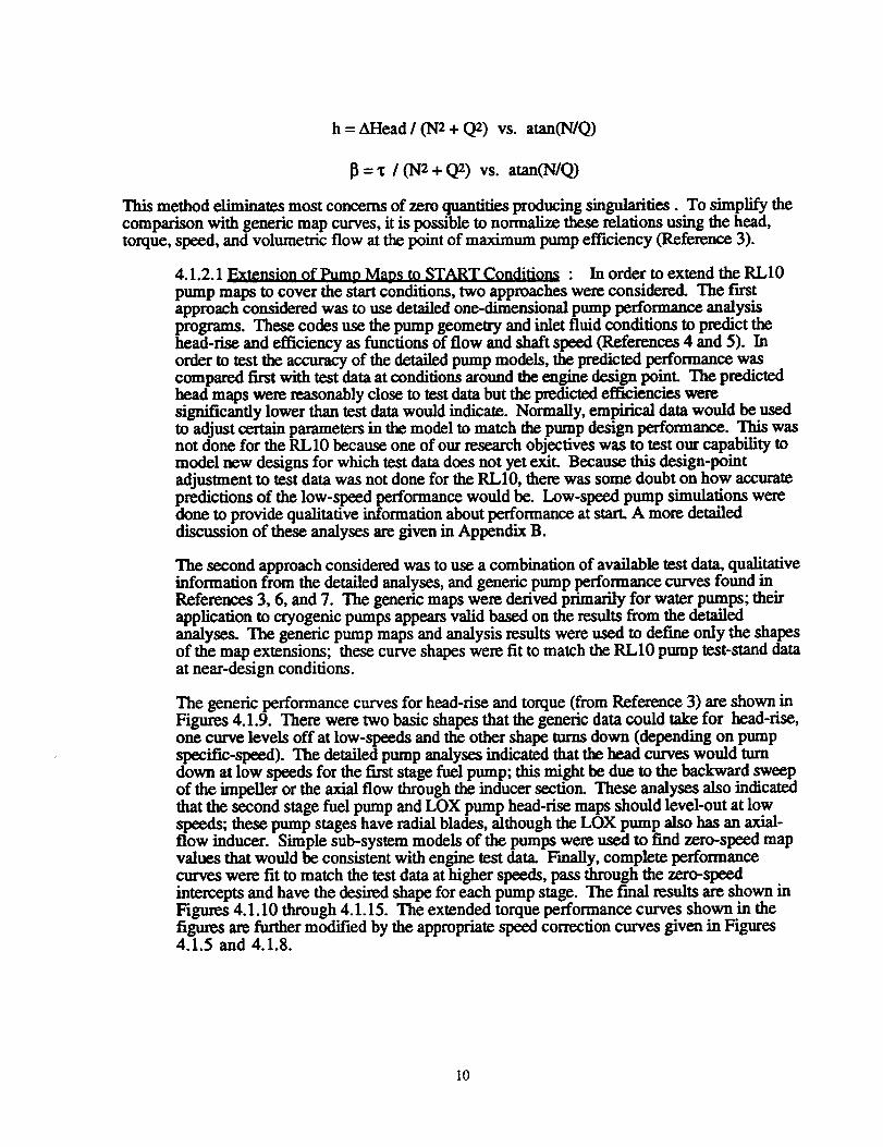
h = AHead / (N2 + Q2) vs. amn(N/Q)

[} = Z / (N2 + Q2) vs. atan(N/Q)

This method eliminates most concerns of zero quantities producing singularities. To simplify thecomparison with generic map curves, it is possible to normalize these relations using the head,torque, speed, and volumetric flow at the point of maximum pump efficiency (Reference 3).

4.1.2.1 Extension of Pump Maps to START Conditions : In order to extend the RL10pump maps to cover the start conditions, two approaches were considered. The firstapproach considered was to use detailed one-dimensional pump performance analysisprogrmns. These codes use the pump geometry and inlet fluid conditions to predict thehead-rise and efficiency as functions of flow and shaft speed (References 4 and 5). Inorder to test the accuracy of the detailed pump models, the predicted performance wascompared first with test data at conditions around the engine design point. The predictedhead maps were reasonably close to test data but the predicted efficiencies weresignificantly lower than test data would indicate. Normally, empirical data would be usedto adjust certain parameters in the model to match the pump design performance. This wasnot done for the RL10 because one of our research objectives was to test our capability tomodel new designs for which test data does not yet exit Because this design-pointadjustment to test data was not done for the RL10, there was some doubt on how accuratepredictions of the low-speed performance would be. Low-speed pump simulations weredone to provide qualitative information about performance at start. A more detaileddiscussion of these analyses are given in Appendix B.

The second approach considered was to use a combination of available test data, qualitativeinformation from the detailed analyses, and generic pump performance curves found inReferences 3, 6, and 7. The generic maps were derived primarily for water pumps; theirapplication to cryogenic pumps appears valid based on the results from the detailedanalyses. The generic pump maps and analysis results were used to define only the shapesof the map extensions; these curve shapes were fit to match the RL10 pump test-stand dataat near-design conditions.

The generic performance curves for head-rise and torque (from Reference 3) are shown inFigures 4.1.9. There were two basic shapes that the genetic data could take for head-rise,one curve levels off at low-speeds and the other shape turns down (depending on pumpspecific-speed). The detailed pump analyses indicated that the head curves would turndown at low speeds for the first stage fuel pump; this might be due to the backward sweepof the impeller or the axial flow through the inducer section. These analyses also indicatedthat the second stage fuel pump and LOX pump head-rise maps should level-out at lowspeeds; these pump stages have radial blades, although the LOX pump also has an axial-flow inducer. Simple subsystem models of the pumps were used to find zero-speed mapvalues that would be consistent with engine test data. Finally, complete performancecurves were fit to match the test data at higher speeds, pass through the zero-speedintercepts and have the desired shape for each pump stage. The final results are shown inFigures 4.1.10 through 4.1.15. The extended torque performance curves shown in thefigures are further modified by the appropriate speed correction curves given in Figures4.1.5 and 4.1.8.

I0

4.1.2.2Extension of Pumo Mars to SHUT-DOWN Conditions : During the engineshutdown, a different combination of off-design conditions appears to exist, including

pump cavitation and reverse flow. Proper simulation of these effects is complicated bytheir interaction with each other. From available test data and simulation output, it appearsthat as the fuel inlet valve closes and the cool-down valves open, the pump first cavitatesdue to a combination of changes in pump loading and cut-off of the inlet flow. The

cavitation causes the pump performance to degrade rapidly until the pump cannot preventthe reverse flow of fluid as it comes backward through the cooling jacket. When thereversed flow reaches the closed fuel inlet valve, however, extreme transients of pressureand flow are created. Similar effects are encountered in the LOX pump during shutdown

as well.

The pump bead and torque performance characteristics during, this period of operation are,of course, not extensively documented in test data. The genenc pump characteristics foundin References 3 and 6 have been used again to extend the .performance .maps for cavitationand reverse flow. The maxima and minima of the curves m this operating regmn werevaried until a reasonable match with engine shutdown test data was achieved. Due tolimitations of schedule and manpower, no attempt was made to predict the post-cavitationand stall behavior of the pumps using the detailed component analysis tools available. It is

likely, in any case, that these tools would require significant modification to examine suchpump conditions; modifications of this kind were beyond the scope of this projecL

The pump map extensions for engine shutdown are included in Figures 4.1.10 through4.1.15. Although the engine start and shutdown models use the same pump performance

maps, the cavitation and reverse flow effects also require additional logic. This logic is notrequired (or even desirable) in the start model. The interested reader is referred tosubroutines PUMPSD, FPASDMP, FPBSDMP and OPSDMP in the model (see Appendix

A) for documentation of these changes.

4.1.2.3 Effects of Density Changes on Pumo Performance Models : The issue ofpropellant phase-change (liquid to gas) has not been adequately adomssed in the genericmaps or detailed analyses described above. It has been noted that using cryogens,numerical instabilities were encountered in the start simulation due to the effects of fluid

changing density in the pumps. Engine test data, although limited, appears to indicate thatthese density instabilities do not actually occur in the pumps during start. In order to obtainstable and reliable calculations, it was necessary to limit density changes within each stage

of the pumps until pumped operation begins. For the start simulation, if the dischargedensity is lower than the inlet density, the discharge pressure is calculated from head-rise

using only the inlet density.

Pdischarge = Pinlet + AHead * pimet

Once pumped operation begins, the standard expression for discharge pressure is used inthe start model:

Paisclaarge = (PinldPinlet + AHead) * pdischarge

During engine shutdown, the propellant densities at the pump inlets may, in reality,

approach zero. Numerical instabilities will arise using either the upstream or downstream

11

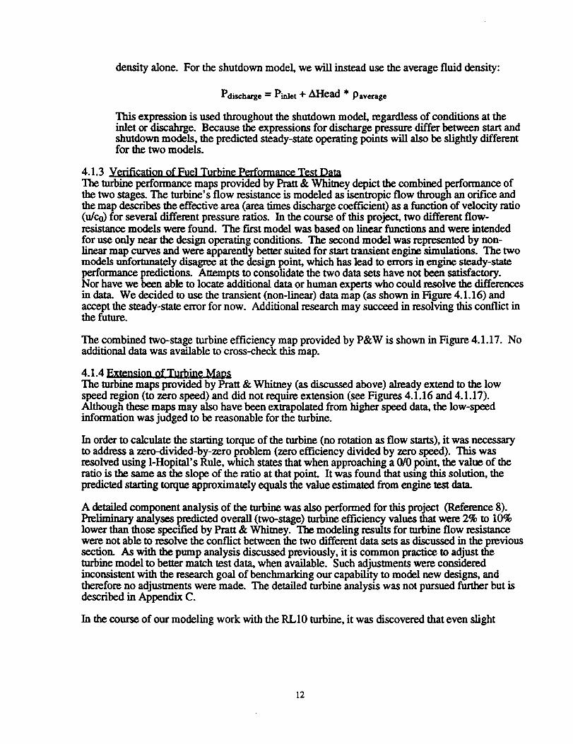
density alone. For the shutdown model, we will instead use the average fluid density:

Pdischarge = ]>inlet + AHead * Paverage

This expression is used throughout the shutdown model regardless of conditions at theinlet or discahrge. Because the expressions for discharge pressure differ between start andshutdown models, the predicted steady-state operating points will also be slightly differentfor the two models.

4.1.3 Verification of Fuel Turbine Performance Test Data

The turbine performance maps provided by Pratt & Whimey depict the combined performance ofthe two stages. The turbine's flow resistance is modeled as isentropic flow through an orifice andthe map describes the effective area (area times discharge coefficient) as a function of velocity ratio(u/Co) for several different pressure ratios. In the course of this project, two different flow-resistance models were found. The fast model was based on linear functions and were intended

for use only near the design operating conditions. The second model was represented by non-linear map curves and were apparently better suited for start transient engine simulations. The twomodels unfortunately disagree at the design point, which has lead to errors in engine steady-stateperformance predictions. Attempts to consolidate the two data sets have not been satisfactory.Nor have we been able to locate additional data or human experts who could resolve the differencesin data. We decided to use the transient (non-linear) data map (as shown in Figure 4.1.16) andaccept the steady-state error for now. Additional research may succeed in resolving this conflict inthe future.

The combined two-stage turbine efficiency map provided by P&W is shown in Figure 4.1.17. Noadditional data was available to cross-check this map.

4.1.4 Extension of Turbine MapsThe turbine maps provided by Pratt & Whitney (as discussed above) already extend to the lowspeed region (to zero speed) and did not require extension (see Figures 4.1.16 and 4.1.17).Although these maps may also have been extrapolated from higher speed data, the low-speedinformation was judged to be reasonable for the turbine.

In order to calculate the starting torque of the turbine (no rotation as flow starts), it was necessaryto address a zero-divided-by-zero problem (zero efficiency divided by zero speed). This wasresolved using 1-Hopital's Rule, which states that when approaching a 0/0 point, the value of theratio is the same as the slope of the ratio at that point. It was found that using this solution, the

predicted starting torque approximately equals the value estimated from engine test data.

A detailed component analysis of the turbine was also performed for this project (Reference 8).Preliminary analyses predicted overall (two-stage) turbine efficiency values that were 2% to 10%lower than those specified by Pratt & Whitney. The modeling results for turbine flow resistancewere not able to resolve the conflict between the two different data sets as discussed in the previoussection. As with the pump analysis discussed previously, it is common practice to adjust theturbine model to better match test data, when available. Such adjustments were consideredinconsistent with the research goal of benchrnarking our capability to model new designs, andtherefore no adjustments were made. The detailed turbine analysis was not pursued further but isdescribed in Appendix C.

In the course of our modeling work with the RL10 turbine, it was discovered that even slight

12

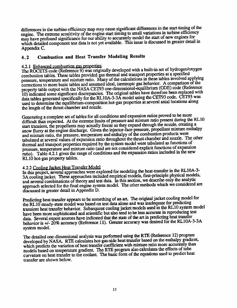
differences in the turbine efficiency map may cause sig.nificant differences, in.the s.h_'t,tin_._ g. of theengine. The extreme sensitivity of the engine start taming to small vanauons m mrome emcaencymay have profound significance for our ability to accurately model the start of new engines forwhich detailed component test data is not yet available. This issue is discussed in greater detail in

Appendix C.

4.2 Combustion and Heat Transfer Modeling Results

4.2.1 Enhanced combustion _as propertiesThe ROCETS code (Referenc_ 9) was originally developed with a built-in set of hydrogen/oxygencombustion tables. These tables provided gas thermal and transport properties at a specified

pressure, temperature and mixture ratio. Many of the calculations in these tables involved applyingcorrections to more basic tables and assumed ideal, isentropic gas behavior. A comparison of the

property table output with the NASA CET93 one-dimensional-equilibrium (ODE) code (Reference10) indicated some significant discrepancies. The original tables have therefore been replaced withdata tables generated specifically for the RL10A-3-3A model using the CET93 code. CET93 wasused to determine the equilibrium-composition hot-gas properties at several axial locations along

the length of the thrust chamber and nozzle.

Generating a complete set of tables for all conditions and expansion ratios proved to be moredifficult than expected. At the extreme limits of pressure and mixture ratio present during the RL10start transient, the propellants may actually freeze as they expand through the nozzle, creating asnow flurry at the engine discharge. Given the injector-face pressure, propellant mixture enthalpyand mixture ratio, the pressure, temperature and enthalpy of the combustion products weretabulated at several values of expansion ratio throughout the thrust chamber and nozzle. The other

thermal and transport properties required by the system model were tabulated as functions ofpressure, temperature and mixture ratio (and are not considered explicit functions of expansionratio). Table 4.2.1 gives the range of conditions and the expansion ratios included in the new

RL10 hot-gas property tables.

4.2.2 Cooling, Jacket Heat Transfer ModelIn this projec-t, several approaches were explored for modeling the heat-transfer in the RL10A-3-3A cooling jacket. These approaches included empirical models, first-principle physical models,and several combinations of theory and test data. In this section, we describe only the analytic

approach selected for the final engine system model. The other methods which we considered arediscussed in greater detail in Appendix D.

Predicting heat transfer appears to be something.of an art. "ll_e orig.in_ jacket cooling model forthe RL10 steady-state model was based on test data alone aria was maaequam for predictingtransient heat transfer behavior. Subsequent cooling jacket models used in the RL10 system model

have been more sophisticated and scientific but also tend to be less accurate in reproducing testdata. Several expert sources have indicated that the state of the art in predicting heat transferbehavior is +/- 20% accuracy (Reference 11). Greater accuracy was desired for the RL10A-3-3A

system model.

The detailed one-dimensional analysis was performed using the RTE (Reference 12) program

developed by NASA. RTE calculates hot-gas-side heat transfer based on the enthalpy gradient,which predicts the variation of heat transfer coefficient with mixture ratio more accurately thanmodels based on temperature gradient. The RTE program also calculates the effects of tubecurvature on heat transfer to the coolant. The basic form of the equations used to predict heat

transfer are shown below.

13

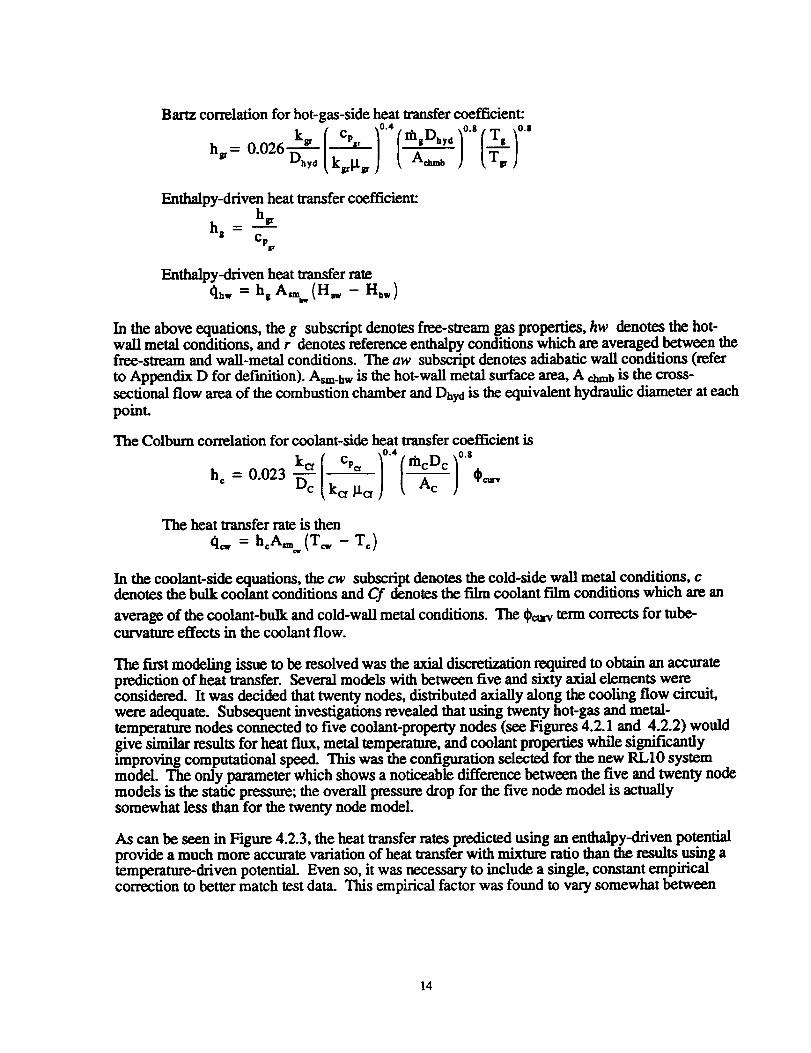
Bartz correlation for hot-gas-side heat transfer coefficient:

Enthalpy-driven heat transfer coefficient:

hs,h s -

Cp_,

Enthalpy-driven heat transfer rote

In the above equations, the 8 subscript denotes free-stream gas properties, hw denotes the hot-wall metal conditions, and r denotes reference enthalpy conditions which are averaged between thefree-stream and wall-metal conditions. The aw subscript denotes adiabatic wall conditions (referto Appendix D for definition). Asm-hw is the hot-wall metal surface area, A cimb is the cross-

sectional flow area of the combustion chamber and Dhyd is the equivalent hydraulic diameter at each

point.

The Colbum correlation for coolant-side beat transfer coefficient is

h, = 0.023 "_c / kct _tcf (--_c J 0_'

Tb.cheat transfer rateisthen

q,,, = h_A_ (T_ - T°)

In the coolant-side equations, the cw subscript denotes the cold-side wall metal conditions, cdenotes the bulk coolant conditions and Cf denotes the film coolant film conditions which are an

average of the coolant-bulk and cold-wall metal conditions. The 0curv term corrects for tube-curvature effects in the coolant flow.

The first modeling issue to be resolved was the axial discretizafion required to obtain an accurateprediction of heat transfer. Several models with between five and sixty axial elements wereconsidered. It was decided that twenty nodes, distributed axially along the cooling flow circuit,

were adequate. Subsequent investigations revealed that using twenty hot-gas and metal-temperature nodes connected to five coolant-property nodes (see Figures 4.2.1 and 4.2.2) wouldgive similar results for heat flux, metal temperature, and coolant properties while significantlyimproving computational speed. This was the configuration selected for the new RL10 systemmodel. The only parameter which shows a noticeable difference between the five and twenty nodemodels is the static pressure; the overall pressure drop for the five node model is actuallysomewhat less than for the twenty node model.

As can be seen in Figure 4.2.3, the heat transfer rates predicted using an enthalpy-driven potentialprovide a much more accurate variation of heat transfer with mixture ratio than the results using atemperature-driven potential. Even so, it was necessary to include a single, constant empiricalcorrection to better match test data. This empirical factor was found to vary somewhat between

14

different tests and engines; an average value of 1.08 was selected for the new engine model. One

possible reason for the required correction is tmcert_tinty.about the effective s_m'fa_ _a_ea of the ncooling tubes exposed to the hot-gas, lne etlect ot orazmg matenat aria me aegxve ui _o,iuu,.uuthrough the braze makes a precise calculation difficult. The empirical correction of 1.08 is alsowithin the +/- 20 % deflation considered acceptable by many heat transfer experts.

The RTE code was also used to determine the flow resistance of each section of cooling jacket.

Comparison with test data indicates the need for an empirical correction to the predicted jacket flowresistance. Here too, the correction factor varies somewhat across different runs and engines; an

average correction of 0.94 was used. Figures 4.2.4 through 4.2.7 show heat flux, metaltemperature, coolant temperature and pressure along the cooling jacket as predicted by the new heattransfer model.

For the RL10 system simulation, a simple boiling heat-transfer model was added to the RTEanalysis results. The transition between boiling heat-transfer and forced convection was assumedto be instantaneous, without any nucleate boiling.

(hc)b°i'i*' = (hc)co'b_ 0.611 + 1.93_tt

where Xtt is the Lockhardt and MartineUi parameter

(see Appendix D for more information).

Analyses indicate that the temperature difference between the jacket metal and fuel at start is sogreat that the fuel will flash immediately and should be treated using a forced convection model;there does not appear to be any appreciable film-boiling in the jacket. In the simulations performedthus far, we have not observed any of the oscillations found in test data and attributed to heattransfer instabilities. These instabilities may be due to extremely localized boiling or two-

dimensional effects not modeled by RTE.

A more detailed description of the RTE analysis and f'drn-boiling model can be found in Appendix

D.

4.2.3 Thrust Chamber Performance CalculationsIt was desirable for modeling efficiency to have simple one-dimensional models of the combustion

chamber and nozzle. Where two and three-dimensional effects were considered significant, they

have been incorporated as tables of correction factors to modify the one-dimensional calculations.

Pratt & Whitney had provided tables of RL10 c*-effieiency (Tic,), ideal specific-impulse 0sp), and

cor e onsfortwo- ensionallo s. Inorderto nchm our d xtendthe range of data provided, we performed several detailed component analyses ot me mjecto,combustion chamber and nozzle using codes available at NASA Lewis.

4.2.3.1 One-dimensional combustion model layout : The model of combustion used in the

RL10 system simulation includes just two nodes (not including heat transfer): one at theinjector face and the other at the inlet to the converging sectio.n of the nozzle;..The static .conditions at the injector face are used to define .the combustion .propem_. _.rom me stalac

pressure at the injector face, the total pressure at the nozzle inlet _ catcutatea,mcl_mgata 1total-to-static conversion and the momentum loss oue to oummg (Kererence t J). _ne t

pressure at the nozzle inlet is then used to calculate the nozzle flowrate.

15

I + M iaj )(P')n "-(P')i.j 1 + ']_VI2,,

(P'r)" = (P')"( 1+ (T-1)M2")(T-_1)2

Since the combustion temperature predicted by CET93 does not include the effects ofvarious combustion and injector inefficiencies, the predicted temperature must be corrected

using TIc*.

T_ = n_- (T_)_,j

4.2.3.2 Detailed modeling of the chamber injector : The ROCCID code (Reference 14)

was used to predict Tic*, which reflects primarily injector performance. ROCCID is a two-dimensional analysis program representing physical principles and general observationsmade in experimental studies. Because the ROCCID code does not include modeling ofribbon swirlers as used in the RL10 design, we attempted to model an equivalenttangential-injection swirler. A number of other design parameters in the model also had tobe guessed, and so there is a significant degree of uncertainty in the ROCCID model of theRL10 injector to begin with. Modeling uncertainties and convergence problemsexperienced with the ROCCID model limited the amount of useful information we could

derive from these analyses. The _c* curves provided by Pratt & Whitney (Figure 4.2.8)

have therefore been used in the new system model instead. The ROCCID modeling resultsare discussed further in Appendix E of this report.

4.2.3.3 blgzzle _t_rformance models : The flowrate of hot-gas through the nozzle wascalculated with a simple one-dimensional model, as shown below.

g (Pr). A_

This correlation gives a result very similar to that using an ideal-gas, isentropic expansionmodel Several different methods were used to estimate the nozzle discharge coefficient(Cd), with similar results. By comparing the effective flow area of the nozzle specified by

Pratt & Whitney (18.85 in2) with the actual physical area of the throat (19.19 in2), it wasdetermined that the Cd should be approximately 0.982. Using a simple one-dimensionalnozzle model, and trimming Cd to match test data for chamber pressure, a Cd of 0.975 wasderived. A two-dimensional Navier-Stokes analysis suggested the Cd should be 0.976,which is a good match with the values inferred above. A Two-Dimensional Kinetics(TDK)(Reference 16) analysis also indicated that the nozzle Cd will vary with chamberpressure and mixture ratio. The variable Cd curves predicted by TDK were not well-behaved, however, and we were unable to adequately explain the variations observed. Itwas decided, based on the above calculations, to use a constant Cd of 0.975 in the RL10

engine system model

The specific impulse Clsp) of the nozzle was also predicted using TDK. The TDK

16

predictions for Isp agree with Pratt & Whitney data near the engine design point, andextend over a wider range of pressure and mixture ratio (Figure 4.2.9). By comparing the

TDK Isp predictions with those calculated using one-dimeusional equilibrium assumptions,

a table of thrust-coefficient efficiency (tic0 was created. This table may be used to correct

the one-dimensional Isp predictions for the influence of two-dimeusional effects (Figure4.2.10). In this way, we were able to leverage a relatively small number of TDK runs witha much more comprehensive table of Isp predictions already generated using the CET93

(ODE) program. The predicted ideal Isp data and two-dimensional Hcf corrections havebeen included in the new RL10 engine system model.

A more detailed description of the analyses discussed here can be found in Appendix E.The results of these analyses, compared with the empirical data provided by P&W, indicatethat we can accurately calculate nozzle performance for a new design. Our ability to predict

the c*-efficiency for a new design is less certain. ROCCID was created to model injectordesigns commonly used today, not the type developed for the RL10 thirty years ago. TheRL10 may therefor be the wrong choice to benchmark ROCCID's accuracy in modeling

new components (those without test data).

4.2.3.4 Two-ohase flow through nozzle : Nozzle flow-resistance is predicted usingdifferent correlations for the lit and unlit cases. When the chamber is unlit, flow is

calculated using an incompressible flow correlation, with the pressure drop limited by the

critical pressure ratio for an ideal gas. This type of correlation has been found to beaccurate in predicting the critical two-phase flow of a low-quality fluid and is also used forthe fuel cool-down valves and LOX injector elements during starL When the chamber is lit,the flow is calculated using the correlation described in the previous section. We have not

been completely successful in developing a single correlation capable of accuratelypredicting the entire range of nozzle flow from the prestart two-phase flow of LOX, to theunlit mixture of warm hydrogen and LOX, to the flow of combustion gases. Differentcorrelations appear to be required for the different operating regimes and the correlationsare not necessarily continuous between the regimes.

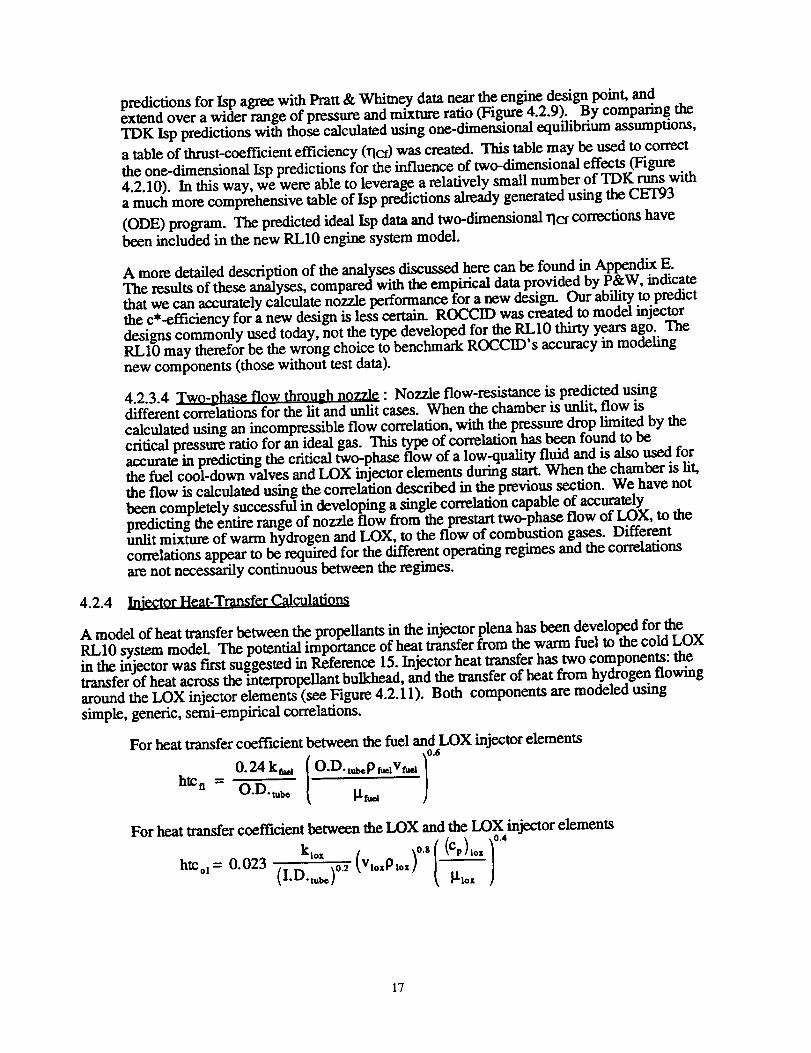
4.2.4 In iector Heat-Transfer Calculations

A model of heat transfer between the propellants in the injector plena has been developed for the

RL10 system model The potential importance of heat transfer from the warm fuel to the cold LOXin the injector was first suggested in Reference 15. Injector heat transfer has two components: thetransfer of heat across the interpropellant bulkhead, and the transfer of heat from hydrogen flowing

around the LOX injector elements (see Figure 4.2.11). Both components are modeled using

simple, generic, semi-empirical correlations.

For heat transfer coefficient between the fuel and LOX injector elements

0.24k_ [O.D.t,a,epfu,avf_a )0.6htc n - O.D.tubo I.tt_a

For heat transfer coefficient between the LOX and the LOX injector elements

htCol= 0.023 (I.D.tub,)0. 2 i'tlox

17

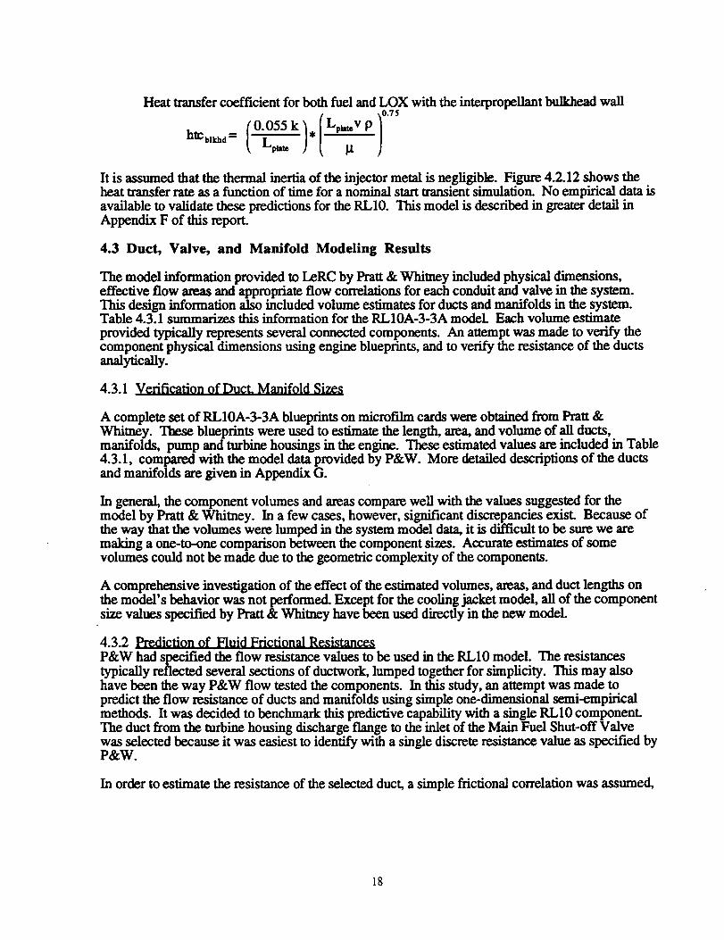
Heat transfer coefficient for both fuel and LOX with the interpropellant bulkhead wall

(0.055 k ). Lp_V P ) TMhteb, ,= (" li

It is assumed that the thermal inertia of the injector metal is negligible. Figure 4.2.12 shows theheat transfer rate as a function of time for a nominal start transient simulation. No empirical data is

available to validate these predictions for the RL10. This model is described in greater detail inAppendix F of this report.

4.3 Duct, Valve, and Manifold Modeling Results

The model information provided to LeRC by Pratt & Whitney included physical dimensions,effective flow areas and appropriate flow correlations for each conduit and valve in the system.This design information also included volume estimates for ducts and manifolds in the system.Table 4.3.1 summarizes this information for the RL10A-3-3A model Each volume estimate

provided typically represents several connected components. An attempt was made to verify thecomponent physical dimensions using engine blueprints, and to verify the resistance of the ductsanalytically.

4.3.1 Vfdfieation of Duct. Manifold Sizes

A complete set of RL10A-3-3A blueprints on microfilm cards were obtained from Pratt &Whitney. These blueprints were used to estimate the length, area, and volume of all ducts,manifolds, pump and turbine housings in the engine. These estimated values are included in Table4.3.1, compared with the model data provided by P&W. More detailed descriptions of the ductsand manifolds are given in Appendix G.

In general, the component volumes and areas compare well with the values suggested for themodel by Pratt & Whitney. In a few cases, however, significant discrepancies exist. Because ofthe way that the volumes were lumped in the system model data, it is difficult to be sure we aremaking a one-to-one comparison between the component sizes. Accurate estimates of somevolumes could not be made due to the geometric complexity of the components.

A comprehensive investigation of the effect of the estimated volumes, areas, and duct lengths onthe model's behavior was not performed. Except for the cooling jacket model, all of the componentsize values specified by Pratt & Whitney have been used directly in the new model.

4.3.2 Prediction of Fluid Frictional Resistances

P&W had specified the flOW resistance values to be used in the RL10 model. The resistancestypically reflected several sections of ductwork, lumped together for simplicity. This may alsohave been the way P&W flow tested the components. In this study, an attempt was made topredict the flow resistance of ducts and manifolds using simple one-dimensional semi-empiricalmethods. It was decided to benchmark this predictive capability with a single RL10 component.The duct from the turbine housing discharge flange to the inlet of the Main Fuel Shut-off Valvewas selected because it was easiest to identify with a single discrete resistance value as specified byP&W.

In order to estimate the resistance of the selected duct, a simple frictional correlation was assumed,

18

equivalent to the Darcy equation as described in Reference 17). The friction factor of the duct wasassumed to be constant of 0.0095, which is consistent with completely turbulent flow in a pipe

with a relative surface roughness of 1.9xl0-S (absolute roughness of 4.6x10-5 inches and diameterof 2.402 inches). Bends in the pipe were replaced by their equivalent lengths, computed using theCrane's software (Reference 18). These analyses are discussed further in Appendix G. Theresistance of the duct derived from this analysis differs approximately 15 % from the value

suggested by Pratt & Whitney. This is an acceptable correlation, considering the uncertainty in

roughness factor.

Although the simple one-dimensional models appear to give reasonably accurate estimates of flowresistance, the results are not suitably accurate for detailed high-fidelity engine models. Two andthree-dimensional analytic tools may increase the accuracy of modeling bends in the pipe, butuncertainty in the wall surface roughness will limit the accuracy for new component designs. Fornew applications, it may be advisable to include the effects of uncertainty in flow resistance as partof the system simulation activities. For the RL10 application, we could use the duct describedabove to determine a surface roughness and apply this value to other components in the system.We have instead elected to continue using the flow resistances specified by P&W in the RL10

system model and have not pursued further analysis on the ductwork.

4.3.3 Modeling 9f Valve Actuator MechanismsMost of the valves in the system involve complex orifice shapes and flow paths. Likewise, theactuators and servo-mechartisms which control the valves are complex, involving a number of

springs, dampers and masses whose characteristics are not generally kno .wn. Dynamic modelingof these actuators, including fluid forces from the propellant flows is considered beyond the scope

of this project. We will therefore continue to use relatively simple functions of time and pressurespecified by Pratt & Whimey and shown in Figures 2.1.2 and 2.1.3. These schedules may bemodified to reflect variations in valve timing as inferred from test data.

4.3.4 Modeling of Critical Tw0-Phase Flow Through a Valve or OrificeThere are a number of situations that have been found where the flow through a particular valve or

orifice may range from liquid to vapor, and from choked (critical) to unchoked flow during thestart and shut-down transients. This is true, for example, in the RL10 fuel cool-down valves,

oxidizer control valve, and oxidizer injector elements. It was necessary to make a more detailed

investigation of these particular components. Past research efforts have met with only limitedsuccess in forming a comprehensive description of the different flow regimes and the transitions

between them (References 19 through 24.). Much of the available experimental research literature

is applicable to steam only. Theoretical treatments (of varying accuracy) typically involve

numerical methods which are not practical for inclusion in a transient system model; these

methods are discussed in Appendix H. The number of independent variables involved in thetheoretical calculations also make it impractical to map the flow for inclusion in the system model.

It was necessary, therefore, to use simple correlations which approximate the results of the more

detailed analyses and which agree with RL10 engine test data. Special cases of the flow

correlations are required for different applications in the RL10 system.

In the new system model, flow through the fuel cool-down valves and the LOX injector are

determined using an incompressible flow calculation (upstream density used) regardless of the

state of the fluid (even if it begins to vaporize). The value of upstream pressure is used, however,

to select the effective pressure drop used to calculate flow, as is described below.

19

in = C d *A* 42g * p_

8p = (Pinlet -Pexit)

* _ip

for Pexit > Psat

_p = (Pialet -Pexit) for Petit < Psat and Pexit > Petit

_p ---- (Pinlet - Psat) for Pcrit > Psat and Pexit < Psat

8p = (Pinlet - Petit) for Pcrit < Psat and Pexit < Petit

Pm = function of Sinlet looked up from tables

¥

P t=I_y+lJ

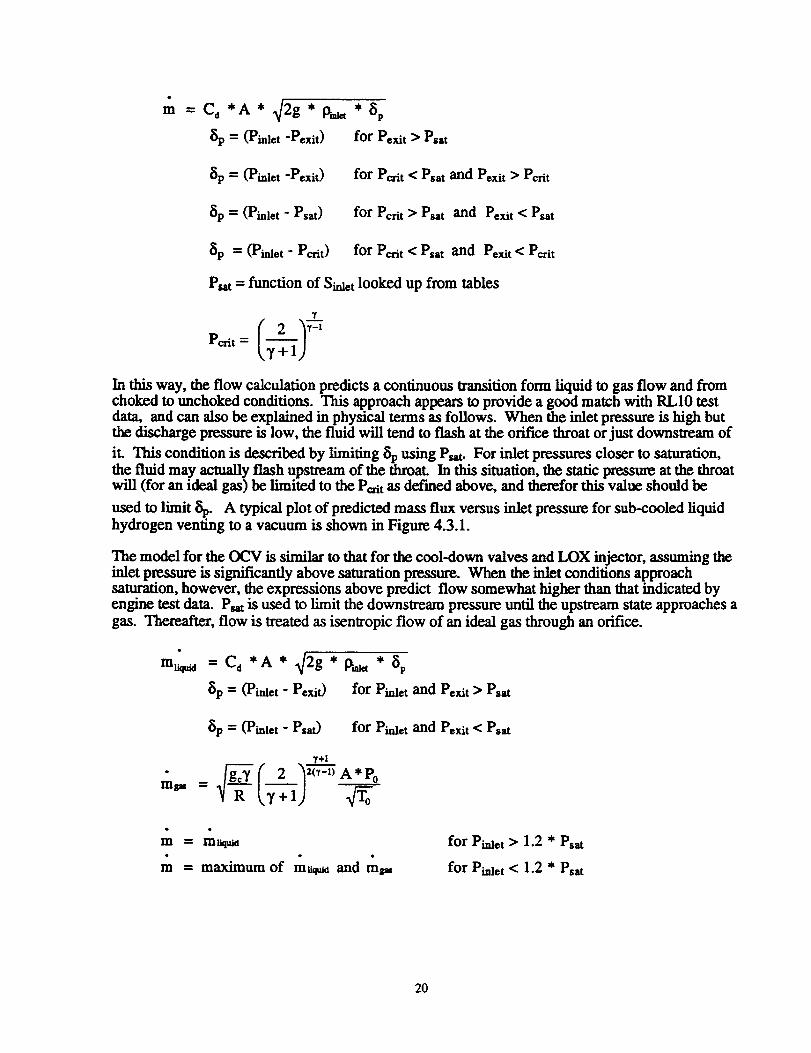
In this way, the flow calculation predicts a continuous transition form liquid to gas flow and fromchoked to unchoked conditions. This approach appears to provide a good match with RLIO testdata, and can also be explained in physical terms as follows. When the inlet pressure is high butthe discharge pressure is low, the fluid will tend to flash at the orifice throat or just downstream of

it. This condition is described by limiting 8p using Pro. For inlet pressures closer to saturation,the fluid may actually flash upstream of the throat. In this situation, the static pressure at the throatwill (for an ideal gas) be limited to the P_t as def'med above, and therefor this value should be

used to limit 5p. A typical plot of predicted mass flux versus inlet pressure for sub-cooled liquidhydrogen venting to a vacuum is shown in Figure 4.3.1.

The model for the OCV is similar to that for the cool-down valves and LOX injector, assuming theinlet pressure is significantly above saturation pressure. When the inlet conditions approachsaturation, however, the expressions above predict flow somewhat higher than that indicated byengine test data_ P_ is used to limit the downstream pressure until the upstream state approaches a

gas. Thereafter, flow is treated as isen_opic flow of an ideal gas through an orifice.

= C d *A* _]2g* P,._,t * 5p

_p = (Pinlet - Pexit) for Pinlet and Pexit > Psat

_p = (Pinlet - Psat) for Pinlet and Pexit < Psat

¥+1

( 2 _2(,-l) A*P0

m = m_id* • •

m = maximum of m_ and m_,

for Pinlet > 1.2 * Psat

for Pinlet < 1.2 * Psat

2O

It is not understood why flow through the OCV should behave differently than the other two-phaseflow components in the engine. The expressions described here provide continuous functions offlow across the phase boundary and agree well with test data.

4.3.5 Model of flow through Venturi

The venturi downstream of the cooling jacket is intended primarily to help provide stable thrust

control using a turbine bypass valve rather than an in-line valve. It is possible that the venturi mayalso serve in general to inhibit system-wide pressure oscillations due to interactions between thecombustion chamber, cooling jacket and turbomachinery. The RL10 venturi is apparently choked

during engine start but not at the normal operating conditions.

Most models of flow through a venturi are based on the total-to-static pressure ratio between theinlet and the throat (References 25 and 26). In the case of the RL10, it is desirable to characterizethe flow based on the pressure ratio between the venturi inlet and discharge (exit from the diffusingsection). By making some assumptions regarding the correlation between inlet-to-throat pressureratio and inlet-to-exit pressure ratio, the performance map shown in Figure 4.3.2 was derived.This model was found to agree well with the data provided to us by Pratt & Whitney. Although

this analysis was not exhaustive, it provided confidence regarding the suitability of the mapprovided for simulation of start conditions. The performance map represents the venturi flow

parameter, FP, which is used to predict mass flow as described below.

For the shutdown transient simulations, inertial damping logic has been added to the venturi modelin order to inhibit oscillations around zero flow once the system is nearly evacuated. Suchoscillations can be induced by numerical instabilities; the inertial damping provides a physically.

meaningful way to damp such oscillations without affecting the normal operation of the ventunmodel.

4.4 The New RL10A-3-3A System Model

The new RL10A-3-3A engine system model was created by integrating component models using

the ROCETS system simulation software (Reference 9). After considering the results of thecomponent analyses, several of these models were selected for inclusion in the new system modelIn other cases, the component data and information provided by Pratt & Whitney has been

integrated directly with the system modeL

4.4.1 Evaluation of Component Models / Integration with New System Model:Not all of our component analysis results have been used in the new RL10 model Some of thecomponent results were judged to be incorrect and so were not included. Other results simplyverified the P&W component data, which was used directly in the system model. Only those

component models which extended the operation range of the model, added flexibility or correctedknown deficiencies in the existing models were added. The list of independent component modelsselected for the new RL10 model are:

1) Pump maps extended to start and shutdown transient conditions using genetic data and

detailed analyses.

21

2) New combustion gas property tables from CET93.

3) New heat transfer modules using enthalpy-driven potentiat% twenty axial nodes for themetal and hot-gas side calculations, connoted to five coolant nodes.

4) A model of heat transfer between the warm fuel and cold oxidizer in the injector

plenum.

5) New model of combustion chamber, including the effects of momentum burning losses.

6) Tables of nozzle specific-impulse and thrust-coefficient-efficiency, generated using

CET93 and TDK computer codes.

7) Revised models of two-phase flow through the fuel cool-down valves, oxidizer controlvalve, and LOX injector elements. Extends the range of pressures for which the modelswill work.

We decided not to use the results of the turbomachinery analyses directly. Nor did we use theresults of the injector performance analyses generated by ROCCID; an empirical table of c*-efficiency has been used instead. In general, we have retained the values of duct and manifold sizeand flow resistance as provided by P&W. We did not attempt to create detailed models of thevalves or actuators, but opted to use the characteristics specified by P&W.

4.4.2 Differences between Start and Shutdown System Models :

One of the original goals of the project was to develop a single model that would predict the starttransient behavior, steady-state performance and shut-down transient behavior of the RL10 engine.This goal has not been achieved as yet. There are currently two system models, one for startsimulations and the other for shut-down. The start transient model is also suggested for making

steady-state performance predictions, although the shutdown model quiescent values are verysimilar. The two models share similar component performance characteristics but differ in thedistribution of dynamic volumes and flow inertia around the pumps and turbine (see shadedmodules in Figure 4.4.1). The additional volumes as inertias were required in the shutdown model

to obtain stable solutions, but lead to transient discrepancies with test data in the start transient

simulations. It appears that during the start transient, the pump flows behave as incompressibleeven though the pressures there appear to be below saturation. If volume dynamics are included inthe pumps, the start simulation exhibits compressible characteristics which can significantly delaythe onset of normal pumped operation. Similar effects appear in the dynamics downstream of theturbine during engine start simulations. Changing the way in which the turbine discharge volumecomponents are distributedappearstoslow the decompression of the turbinedischargeas the

FSOV opens during start. This reduces the starting torque and slows the start acceleration. Due tolimitations of schedule and data, it was decided to maintain two separate models rather than

attemptingto resolve the dynamic modeling differences.

5. MODELING UNCERTAINTIES

Before discussing the results of the system simulations, it is important to note sourcesof modelinguncertaintywhich will affect our ability to model any given test or flight engine fn-ing. There areseveral sources of modeling uncertainty which effect the RL10 model's ability to simulate anygiven firing. These uncertainties can be divided into four categories: 1) uncertainty in hardwarecharacteristics, 2) uncertainties in valve dynamic behavior, 3) uncertainties in engine initial

22

conditions and boundary conditions, and 4) uncertainty in main chamber ignition delay.

5.1 Hardware Uncertainties

In addition to modeling uncertainties due to insufficient data (such as fluid resistances and pumpstall characteristics), there are some elements of the hardware which may vary from en .gine to

engine. Information regarding these hardware variations is not readily available for a given test orflight engine, making it difficult to account for such differences in modeling the behavior of that

particular engine.

One component which may vary from engine to engine is the fuel pump discharge orifice classused. This orifice is chosen according to knowledge of components in the engine and, onoccasion, trim runs of the engine. The choice of orifice class is designed to _ variations innominal engine performance (thrust, Isp). It is not clear, though, how these variations mightaffect the start or shutdown transient behaviors.

Certain apparent variations in heat wansfer coefficients and cooling jacket fluid-resistance have alsobeen noted. It has been suggested that the effects of variations in the tube brazing may be thesource of variations in heat transfer from engine-to-engine. These variations are not critical to

successful engine operation but may perceptibly alter the engine time-to-accelerate.

The fuel pump cooldown valves are another area of uncertainty. It has been suggested that thesevalves have a discharge coefficient (Cd) which may he different for ground-test and flight becauseof differences in the size of the duct which vents the cooldown flow overboard (Reference 27). Inthe RL10 model, the discharge coefficient is set at 0.6 for ground-test and 0.8 for flight. Thesevalues were chosen based on discussions with engineers at Pratt & Whitney but no real calibrationdata is available to verify these values. Figure 5.1.1 shows the variation in simulation for an

engine first start with different Cd values between 0.6 and 0.9. In the case of the shutdown

transient, the model actually assumes that the. dischar.ge coefficient may. change wi'th tinae _ _o_discharge duct fills and cools. This assumplaon was inferred from engme test aata, aria hasbeen verified either. The cooldown valve resistances are a major factor in both the start andshutdown simulations, and the uncertainty in these values may therefore be a significant source of

any discrepancy noted between simulated and measured data.

The running torque of the RL10 turbopump (fuel and LOX combined) is another accepted sourceof engine-to-engine variation. These values are not generally measured for each engine but paststudies (Reference 28) have shown that the torques vary from 8 to 36 lbf-in. The same nominaavalue of 20 lbf-in torque relative to the fuel pump shaft has been used for all the simulations run for

comparisons with flight and test data. It is uncertain what the actual values of running torque werefor the test and flights considered but it is unlikely that the values were precisely 20 lbf-in.Variations in the simulated start of an engine with different running torques is shown in Figure

5.1.2.

5.2 Valve Uncertainties

The transient behavior of the engine in both start and shutdown is largely determined by the

opening and closing of valves. If there are variations in the time and rate at which these valvechanges occur, the acceleration of the engine will vary also. The assumed opening and closingschedules for the start and shutdown simulations are shown in Figures 2.6.1 and 2.6.2.

It has been acknowledged that variations in valve timing actually do occur (Reference 26). This

23

may be due to timing differences in command signals relative to ignition, dynamic responsevariations of the pneumatic actuation system, and small differences in the dynamic behavior of theservo-mechanisms which controlthefuel pump InterstageCooldown Valve (FCVI), Oxidizer

ControlValve (OCV) and ThrustControlValve O'CV). In some cases,the opening and closingtimes of valve.scan be inferredfrom testdata.In most cases,however, thisisnot possiblebecause

of insufficientdataand limitationsinthe dynamic response ofthesensors.

Of all valves in the engine system, the OCV poses the greatest uncertainty. This valve is servo-actuated by the pressure rise across the LOX pump and the point at which it opens is the singlemost significant factor in determining when the chamber pressure rises to its full power level. Themodel describesthe opening of the OCV by a simplefunctionof pump delta-P,with limitson the

slew ratetopreventinstantaneouschanges and toggling.A dynamic model of _ actuatorisnot

availableand thedynamic response ofthismechanism may, infact,be differentfrom one enginetothenext. Figure5.2.1shows thevariationinengine starttimingwith differentassumed OCV

opening pressuresbetween 50 and 150 psid.Figure5.2.2shows the inferredOCV schedulebased on back-calculationfrom testdata;itshouldbe noted inthiscase,however, thatthe data-

reductionmodel did not account forsensorlags,and assumed thatthebypass valveopened atthe

correct time.

5.3 Uncertainty of Initial Conditions

The temperature of thecombustion chamber, nozzleand coolingjacketatthe beginning of theengine start sequence is an important factor in the engine time-to-accelerate. Unlike the engine inletpressures and temperatures, there is no reliable measurement of jacket temperature for any giventestorflight.Temperatures thatare measured on theengine generallyshow falsereadings beforestartdue to interactionwith theambient environment, metal conductionwith othercomponents,

and the absence of propellantflow atthattime. The initialtemperatureof thecoolingjacket,ducts,

manifolds,and othercomponents issimply guessed,oftenbased on limitedinformationfrom past

testing.

In the RL10 model discussed here, the temperature of the cooling jacket is assumed to be a uniform

540 degrees R because that is the typical ambient temperature in Florida (which is applicable forboth ground-tests at Pratt & Whitney and launch from Cape Canaveral). This initial temperature isalso suggested to include the effects of a warm nitrogen purge in the vehicle interstage adaptor (650R gas). The temperature of the cooling jacket metal for second bums is assumed to be uniform350 degrees It, based on assumptions about the average metal temperatures after the previous

firing. The cooling jacket inlet manifold is assumed to be at 200 R because the inlet manifold isexposed to some contact with the fuel pump cooldown flow before start. All other components inthe system are assumed to be in thermal equilibrium with the propellant flows at all times (no heattransfer, fully conditioned engine before start). Clearly, these assumptions are rather arbitrary andare likely to be in error to some degree for any given firing. Such assumptions are necessary dueto insufficient information regarding the actual ambient conditions and pre-start conditioning. The

RL10 system model does not include a complete thermal model of the engine sm_cture that wouldbe required to simulate the pre-start conditioning process.

Figure 5.3.1 shows the variation in engine start due to different assumed chamber temperaturesbetween 250 and 500 R.

5.4 Uncertainty in Ignition Time

For the simulations considered here, the ignition time is set to agree with the measured data.

24

Predictingtheignitiontime as wcU would requirean ignitionmodel, which iscurrentlynotavailable.An empiricalmodel would probablybe the.bestsolutionifsuch predictivecapab_tics

arc desired in the future. For the time being, we must be content to predict the start g_ven a Known

range of ignition times between 0.10 and 0.40 seconds after the IVIES signal. The variation of starttime with ignition delay is shown in Figure 5.4.1.

5.5 Interaction between uncertain parametersBecause the RL10 (or any expander cycle rocket engine) is a system of highly interdependentcomponents, the variation in engine behavior due to the uncertainties described above cannot begauged without considering how the variations in components might interact. In order to

adequately map the range of en.gine acceleration times .with inl.et conditions, inila_l con__fiomame_andrunning torque, valvecharactensucs,etc.,a largematrix ot stmutate_ runs must oe pcnothe resuIts appropriately analyzed. A study of this type was previously performed by Pratt &Whitney and the Aerospace Corporation (Reference 28), but was not undertaken as part of this

project.

6. COMPARISON OF SYSTEM MODEL PREDICTIONSWITH TEST DATA

The start and shutdown models have been run to simulate specific ground-test and flight engine

firings. In this section, the simulation results are compared with the measured engine data.

6.1 Verification of Steady State Performance Predictions :Ten test cases are considered for the steady-state performance predictions. Five tests are based on

different quiescent operating points for a single ground-test run of a single engine (Engine P2087,Run 2.01, October 4,1991). The other five tests are based on the final state of five start transientdata sets (five different ground-test runs) of a single engine (P2093). Flight data has not beenincluded in this comparison because insufficient data exists to determine the mixture-ratio and trim

position of the OCV for those firings. In simulating the first five tests, the OCV position wasvaried to achieve the desired mixture ratio at each operating point; the actual test was configured to

allow changes in the OCV position as well. In the other five tests, it is believed that the OCVwould have been set to a single position. Although the OCV trim on the simulations indicated

different OCV positions in each of these five tests, an average position was chosen and used for allfive runs. A comprehensive performance prediction for a typical case is shown in Table 6.1.1. Ingeneral, only a very few parameters are measured on actual engine firings (14 parameters onground tests, 8 in flight). The engine inlet pressures and temperatures, and the combustionchamber pressure were typically treated as inputs to the model; the other parameters were calculatedby the model. A statistical comparison, showing the distribution of error between the measuredand predicted parameter values in the ten ground-test cases, is shown in Figure 6.1.1.

The model predictions match the measured values to within 10% for all parameters on all tests (atotal of 90 values). Most predictions are within 4% of the test results. The most pronounced andconsistent sources of error are in the turbine inlet temperature and the pump discharge pressures.

The difference between the predicted and measured turbine inlet temperatures may be attributed toheat transfer uncertainties in the combustion chamber cooling jacket (discussed in section 4.2.2 of

this report).The errors in the pump discharge pressuresappeartobe associatedwith turbopump

speeds that are consistently lower than measured. This discrepancy in speed is most likely due tosmall errors in the turbine maps and cooling jacket model; these errors cannot be easily corrected

for without adversely affecting the predicted start behavior. It was found, in fact, that the turbine

performance maps recommended for predicting steady-state performance are not the same as thoserecommended for simulating engine start. It was decided that the turbine maps suggested for start

25

transient modeling would be used throughout, and the steady-state error accepted.

6.2 Verification for Start Transient Simulations :

Four engine fn'ings have been plotted in order to compare model predictions with measm_ data.Figures 6.2.1 through 6.2.8 show the predicted and measured start transient of a single ground-test first-burn. Figure 6.2.9 shows chamber pressure for a ground-test second bum of the sameengine. Figures 6.2.10 through 6.2.12 show an Arias/Centaur (AC-72) flight f'wst-hum and Figure6.2.13 shows the second-bum for a different flight (AC-74). In each of these runs, the ignitiontime has been set in the model based on examination of the test or flight data. The differencebetween ground-test and flight engine simulations is the value chosen for the fuel cooldown valvesdischarge coefficient (which reflects differences in the vehicle and test-stand ductwork). Thedifference between first and second bum simulations is the assumed initial temperature of thecombustion chamber metal. These variations were discussed in greater detail in section 5.3 above.

As these figures indicate, the start model generally matches the measured time-to-accelerate towithin approximately 230 milliseconds, using only guesses for initial temperatures, bearingfriction, valve schedules and other factors which may very from run to run and from engine toengine. Table 6.2.1 gives the predicted vs. measured time-to-accelerate (defined here as the timefrom MES at which the chamber pressure reaches 200 psia) for six ground-test and three flight-engine firings. One of the flight simulations is off by 280 msec (rather than 230 msec), but thisappears to be aberration relative to other flight-engine starts; it is likely that the engines for thisflight are different in some ways other than their inlet conditions (see section 5 above for adiscussion of uncertainty). The model correctly predicts start variations due to different engineinlet conditions, initial thermal conditions, and differences between ground and flight hardware.

The reader may note that there are some transient differences between the predicted and measuredovershoot in chamber pressure during start, before the engine reaches its quiescent state. Thesmaller oscillations evident in the test data are due to oscillations of the TCV servo-meehanism.

The simulation does not include a model of the actuator dynamics, but the valve is scheduled toopen as a linear function of combustion chamber pressure; it initially overshoots chamber pressurebut does not oscillate. In several cases, the simulation exhibits some rather sharp transients beforereaching steady-state; these appear to be due to volume dynamics in the LOX pump inlet duct. Asthe OCV suddenly opens and the LOX system pressurizes, the simulation may predict oscillationscaused by fluid compression, inertia, and phase changes. These lransients, which are not evidentin the test data, may occur in the simulations because the OCV servo dynamics are not included inthe model. These transient differences between predictions and test are not considered sefions;they may be eliminated ff models of the TCV and OCV actuators are developed in the future.

To demonstrate one potential application of the system start model, Figure 6.2.14 shows thepredicted metal temperature of the combustion chamber just upstream of the throat (its hottestpoint) during start. This parameter is not measured, even in ground tests. The temperature in thiscase peaks at around 1875 R, which is a well below the melting point of the silver throat insert.Information of this kind can be used to help determine component wear and to assess the impact ofoperational or hardware changes to the engine.

The new RL10 system model may also be used to explore new control options for the engine.Enhancements to the engine's control system are currently being developed, including an electroniccontroller and electro-mechanical actuators for the valves. These changes will enable much greatercontrol flexibility. As a small demonstration of the benefits that the new control system mayafford, the RL10 engine model was used to simulate modifications to the OCV timing during start.The trigger pressure and valve slew-rate were both altered in order to increase the differential

26

pressure across the ignitor GOX supply line. The goal was to reduce the danger of supply l_aefreeze-up, which may occur if combustion products (water) back-flow into the supply line duringstart.. The results of the simulation, shown in Figure 6.2.15, indicate that this approach has the

desired effect, although the OCV control could be further optimized to maintain the desired delta-P

throughout the start operation.

6.3 Verification of Shutdown Transient Simulations :

Two firings have been used for comparison between model predictions and measured data. RL10engine shutdowns do not appear to have any distinct feature analogous to the time-to-accelerate forstart transients. Although there are subtle variations in the rate of deceleration, the nature of thesedifferences is not as well understood as in the case of engine start.

Figures 6.3.1 through 6.3.8 shows the predicted vs. measured shutdown for a ground-test engine.Figures 6.3.9 though 6.3.14 shows similar comparisons for a flight engine. As described in theprevious section, the difference between ground-test and flight engine models is the assumeddischarge coefficient of the fuel pump cooldown valves. Figures 6.3.15 and 6.3.16 show

predicted and measured pump speed for the various p.re.diced shut.dow n Iran.sients for _u._._lalground-test firings, giving some indicataon of the vanataon aug to nuet conomons ano

operating point.

The RL10 shutdown model has captured many interesting effects that occur during shutdown. In

Figure 6.3.3, for example, the model and measured .da_ both show a c l_raeteristic dip, .'_ri_._and _then falloff in the fuel venturi upstream pressure. Ires zeamre _s causeo oy me uynamtc mterazuuuof the fuel pump cooldown valve opening and main fuel shutoff valve closing. In Figure 6.3.5,the jump in pump inlet pressure and the shape of the fuel pump discharge pressure curve (notshown) are both due, in part, to reverse flow through the fuel pump.

From inspection of the plots, it appears that there are still some unresolved differences between thepredicted and measured engine deceleration rates. In comparing the start and shutdown predictionsrelative to test data, the reader should note that the time scales of the shutdown wac.e_ are much

smaller than those of the start transient plots.

The new RL10A-3-3A shutdown model developed here can be used to simulate the effects of

various operating scenarios on the engine and vehicle. For example, it may be possible to 'soften'the shutdown transient and minimize the potential for engine damage. The model may also be used

to explore shutdown options which will minimize thrust and impulse imbalance for vehicles which

use multiple engines.

7. DISCUSSION OF MODELING RESULTS

The technical results of the RL10 modeling project are presented in the previous sections of this

report In this section, the significance of these results is discussed.

7.1 Discussion of Turbomachinery Investigation

The available literature on the low-speed operation of pumps appears to be fairly consistent.

Techniques for matching the low-speed generic maps found in the literature to the high-speed test

data are qualitative at best, however.

Available computer programs for predicting turbine and pump performance based on component

27

geometry and operating conditions were also considered in the RLIO modeling project. Mostcodes of this type are not intended to predict the dissipative operation of pumps at very low speedsnor the reverse flow during pump surge. It is common practice to first anchor component modelsusing test-stand data around design point, before using these models to predict off-designbehavior. This a priori requirement for test data will make it difficult to accurately predict theperformance of new component designs, for which such data is often not available. Even whentest data cannot be used to tune the models, however, the results may be sufficiently accurate to

provide designers with useful information. It appears that there is still a significant amount ofwork required to develop accurate first-principle models of cryogenic turbopumps, especially fortransient simulations. The tools used here to model the RLIO turbomachinery are still in thedevelopment and technical review phase, and subsequent versions of these tools may be moreaccurate without requiring adjustment with test data. This subject is discussed in greater detail inAppendices B and C.

It has also been noted that relatively small differences in curve-fits to the turbine efficiency maps atlow speeds can create significant differences in the engine time-to-accelerate. Small variations inturbine efficiency are amplified by system interactions; the turbine drives the pumps, which in-turndrive fuel through the cooling jacket to provide power for the turbine. Given the scarce amount ofdata in the low-speed region, the selection of the proper curve fit through the available data istherefor critical. This effect also has profound implications for our efforts to predict the turbineperformance from first-principles. The sensitivity of the system start tinfmg to the turbineperformance makes almost _ predictive error unacceptable.

7.2 Discussion of Combustion and Heat Transfer Investigation

The three modeling issues which arose regarding the cooling jacket heat transfer are 1) the numberof axial heat transfer nodes to be used, 2) the variation of hot-gas properties along the chamber andnozzle, and 3) the variation of heat transfer properties with changes in mixture ratio.

It seems clear from Figure 4.2.6 that the use of differential enthalpy to predict hot-gas-side heattransfer ('enthalpy-driven potential') is significantly more accurate than the correspondingtemperature-driven heat transfer model. This method accounts for variations in mixture ratiowithout requiring an explicit empirical correction for that effect. A single (constant) empiricalcorrection of 1.08 was still required to match test data.

It is uncertain what benefits were gained from including more heat transfer nodes and non-idealexpansion effects. Certainly, more nodes will give a more accurate axial distribution of metaltemperatures and heat fluxes along the chamber and nozzle. On the other hand, the overall coolantheat pick-up and pressure drop prediction may not be any more accurate using more nodes; theoverall pressure and temperature change are the only quantities that really affect systemperformance. A comprehensive comparison of the system-level effects of node distribution onpredicted engine performance was not within the scope of this project, however, and the hybridmodel with twenty metal nodes and five coolant nodes was used in the new system simulations.

An attempt was also made to predict the RL10 combustion efficiency using the ROCCTD code.The results of this analysis were somewhat uncertain and require further study. It appears thatengineering judgement and estimates for some design parameters is still required to model newdesigns. Perhaps some methodology or integration with other analyses tools can be made that willrefine the modeling process and eliminate modeling uncertainties. TDK and Navier-Stokesanalyses were performed to predict the nozzle specific-impulse and discharge coefficient. TheNavier-Stokes analysis confm'ns that the nozzle Cd at engine design conditions is approximately

28

0.98, as was also inferred from test data. The TDK analysis appears to accurately predict specific

impulse, but the results for discharge coefficient and heat flux were somewhat suspect.

7.3 Discussion of Duct, Manifold and Valve Investigation

Estimates of duct and manifold volumes, areas, and lengths based on RL10 blueprints show somedifferences from the values suggested by Pratt & Whitney. Some of the discrepancies may be due

to complex geometries which cannot be estimated properly from the blueprints. In other cases, thevalues given by Pratt & Whitney may be less accurate than our estimates. For the new model, ingeneral, the volumes, areas and lengths provided by P&W are used.

We have successfully verified the resistance of the duct from the turbine discharge to the main fuelshut-off valve to within +/- 20%. Given the uncertainties in duct surface roughness and the

complex series of bends and elbows in the duct, there appears to be no advantage in predicting theresistance of all ducts in the system. The only reliable method to accurately characterize flowresistance is still to run flow tests. More sophisticated flow modeling tools may also be used to

improve accuracy of the predicted flow-resistances, but the surface roughness must still be known

precisely.

For the new system model, two-phase critical flow is modeled using simple one-dimensional,homogenous correlations. Different correlations are used for the fuel cool-down valves, theoxidizer control valve and the LOX injector elements depending on the propellant vapor pressure

and range of operating conditions encountered in each case. Two-phase flow may actually involvea number of complex physical effects. Not all of these effects, it appears, lend themselves to

elegant theoretical models or accurate predictions.

7.4 Discussion of System Model Simulation Results

Overall, the new version of the RLI0 system model appears .to predict the start acceleration, -ata"steady-state performance, and shutdown behawor of the engine accurately (compared to test a ).The simulated variations in the time-to-accelerate due to changes in engine inlet conditions, ignition

time, and the initial thermal conditions track the varia.tions observed .'.mtest data._ In general, _eLtmodel predicts the time to accelerate to within approximately 230 milliseconos ot tlae test ana mgndata results under the conditions considered. Steady-state performance predictions matchmeasured values to within 10% in all cases (and matched most values within 4%). The RL10shutdown model successfully predicts the transient characteristics of the engine shut-down

process, including effects due to reverse flow in the pumps.

8. CONCLUDING REMARKS

The goals of the RL10A-3-3A Modeling Project have been accomplished. Analyses wereperformed for all major engine components, and many of the results from these studies have beendirectly incorporated into the new system modeL Other analysis results have simply supported theinformation already found in the baseline model, giving us greater confidence in those aspects ofthe model. Still other parts of the study have tested the limits of our analytic tools and expertiseand found them somewhat wanting. The project has therefore helped to benchmark the detailed

component analysis software and techniques currently being used and developed in the SpacePropulsion Technology Division at NASA Lewis Research Center. The information derived fromthis research may be used in refining these analysis tools in the future.

In addition to providing an improved system model of the RL10, the analyses performed under this

29

project have given us a better understanding of the engine system in general. The effects ofvarious design and operational uncertainties on engine performance have been elucidated throughsimulation, and many of the transient features visible in test data have been explained using thenew system model as well.

The RL10A-3-3A engine system models developed here are available to NASA and other users forstudying the behavior of the engine under a wide range of operating conditions. The models canbe used to assess various mission scenarios, to investigate test and flight anomalies, and toevaluate potential design changes. These models could also be modified to simulate RL10A-4 and

RL10A-4-1 engine configurations.

Finally, this project gives an excellent perspective on the current limitations of engine systemmodeling from first principles. In any new engine system being considered, there will likely beseveral unknowns and uncertainties that will require test data to resolve. A priori modeling of a

given design can only give a possible range of quantitative predictions, based on uncertainties incomponent performance. System modeling of a preliminary design can serve to flag issues whichstem from such uncertainties, but we cannot expect such models to precisely predict transientbehavior before comprehensive component test data are available. Once the uncertainties incomponent behavior have been resolved, highly accurate and precise system models can becreated.

30

9. RECOMMENDATIONS for FUTURE RESEARCH

On the basis of this study, several recommendations can be made regarding future work whichwould improve our understanding and models of the RL10A-3-3A rocket engine. No specificwork elements are currently planned to accomplish these additional goals.

I. Once code developments arecompleted,thePUMPA and TURBA codes shouldbe

used torepeattheanalysisofthe RL10A-3-3A turbomachinery. Ifthe new

predictions axe found to match closely with test data, the models can be used toexamine the very low speed performance of the turbopumps. If the new predictionsstill show some disagreement with the test data near the component design points,

appropriate empirical corrections may also be applied before analyzing the low-speed performance characteristics.

2. The work to combine the Rostefmski models of the pump impellers with two-phasecritical flow models of the exit diffusers should be pursued further.

3. Research should be expanded, in general, in the areas of transient and far off-

design pump operation, including cavitation, stall, reverse flow, etc. Accuratemodels of these effects do not appear to exist.

4. A more detailed one or two-dimensional model of film boding in the cooling jacket

should be developed. This model should be capable of accurately predicting the

amp.litude and frequency of pressure oscillations caused by film boiling duringengine start.

5. Some investigation regarding the source of engine-to-engine variation in coolingjacket heat transfer coefficient and fluid resistance should be made.

6. The ROCCID code should be modified to better model the RL10 injector elements.ROCCID should also be modified to allow far off-design conditions (such as

during engine start and shutdown.

7. The Navier-Stokes code used to determine the design-point nozzle discharge

coefficient should be used to map Cd at off-design conditions as well.

8. TDK/MABL should be considered to improve the accuracy of the heat transfer

correlations using in the RL10 model

9. A thorough study should be made on the two-phase flow of cryogens, includingtransition from choked to unchoked behavior. Only limited data and theoretical

treatments appear to exist on this subject.

10. A detailed transient analysis of duct and manifold p._g should be performed,especially for the LOX injector plenum during en .glne start. The abrupt transitions

to completely incompressible flow, as predicted using a simple lumped parametermodel, are probably not realistic.

11. A comprehensive chili-down model for the RL10 engine should be developed toaccurately predict the initial conditions for the start transient. Particular attentionshould be made to modeling the turbopump and the entire LOX feed system.

31

12.

13.

A model of the RLIO ignitor should be developed that win accurately predict thetime of main-chamber ignition with respect to the MES signal.

A study should be performed using the current RL10 engine system model topredict the variation in time-to-accelerate due to uncertainty in initial conditions,engine inlet conditions, turbopump drag torque, etc. (similar to the results ofReference 28 but with additional parameters).

32

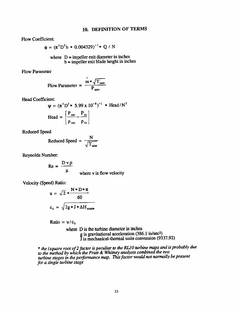
10. DEFINITION OF TERMS

Flow Coefficient:

t) = (lr2D2b * 0.004329) -1. Q/N

where D = impeUer exit diameter in inchesb = impeller exit blade height in inches

Flow Parameter

Flow Parameter -P ialet

Head Coefficient:

_t = (_2D2" 5.99x 10-') -_

Head = Pout Pia ]

P out P in J

• Head/N 2

Reduced Speed

NReduced Speed = - _r-_-----

4li .

Reynolds Number:

Re-Dvp

IX where v is flow velocity

Velocity (Speed) Ratio:

N*D*n

60

c 0 = _/2g*J*AH**=a e

Ratio = u/c o

where D istheturbinediameterininches

g isgravitationalacceleration(386.I in/sec2)J ismechanical-thermalunitsconversion(9337.92)

* the (square root of 2factor is peculiar to the RLIO turbine maps and is probably dueto the method by which the Pratt & Whitney analysts combined the twoturbine stages in the performance map. This factor would not normally be present

for a single turbine stage

33

11. ACKNOWLEDGMENTS

This project was performed under contract (NYMA contrac0 and grant (U.Memphis grant);

funding was provided by the Launch Vehicle Project Office and Space Propulsion TechnologyDivision at the NASA Lewis Research Center.

The author would like to acknowledge the participation of the project team mambers for theircontributions to this endeavor:

Mr. Tom Tomsik (NASA LeRC-5320) : for performing both empirical and detailed

theoretical analyses of the RL10 cooling jacket.

Mr. Joseph P. Veres (NASA LeRC-5320) : for obtaining turbomachinery test-stand dataused in model verification, and for his detailed pump and turbine component analyses

using the PUMPA and TURBA codes.

Dr. Kenneth Kaczynski (NASA LeRC-5320) : for performing detailed analyses of the

RL10 combustion chamber and nozzle using the ROCCID code, TDK, and his own

Navier Stokes-analysis code.

Mr. Douglas Rapp (NYMA Inc. - LeRC SETAR) : for generating the extensive tables ofcombustion gas properties required to model the RL10 combustion chamber, nozzle, and

cooling jacket.

Mr. Dean Scheer (NYMA Inc. - LeRC SETAR) : for performing analyses of the RL10

pumps using the LSISO program, and using his own code based on methods suggested inReference 5.

Mr. AI Pavli (NYMA Inc. - LeRC SETAR) : for developing a model of heat transfer in

the RL10 injector plenna, as well as providing invaluable information on other aspects ofRL10 combustion and heat transfer.

Mr. Bill Tabata (NASA LeRC-5320) : for providing general information and guidance

throughout the project. He acted as liason between LeRC and Pratt & Whitney for

obtaining data, information, and bluebrints. He also helped to review this report.

Dr. John Hochstein (University of Memphis) : for his assistance in developing two-

phase flow models for the Fuel Cool-down Valves.

Other researchers at NASA LeRC and its contractors, too numerous to list here, also provided

assistance on elements of the component and engine-system modeling. Their contributions are

gratefully acknowleged also.

We would also like to recognize the participation of Pratt & Whitney (West Palm Beach, Florida)and Martin Marrietta (Denver, Colorado). They provided data, information and blueprints on the

RL10 which were critical to the success of this project.

34

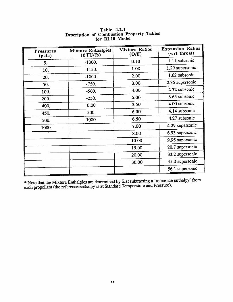
Pressures

(psia)

.

10.

20.

50.

Description

Table 4.2.1of Combustion Property Tables

for RL10 Model

Mixture Enthalpies

(BTU/lb)

-1300.

-1150.

-1000.

Mixture Ratios

(O/F)

0.i0

1.00

2.00

3.00-750.

Expansion Ratios(wrt throat)

1.11 subsonic

1.29 supersonic

1.62 subsonic

2.35 supersonic

100. -500. 4.00 2.72 subsonic

200. -250. 5.00 3.65 subsonic

400. 0.00 5.50 4.00 subsonic

450. 500. 6.00 4.14 subsonic

6.50

7.00

8.00

500.

1000.

1000.

10.00

15.00

4.27 subsonic

4.29 supersonic

6.93 supersonic

9.95 supersonic

20.7 supersonic

20.00 33.2 supersonic

30.00 45.0 supersonic

56.1 supersonic

* Note that the Mixture Enthalpies axe determined by fLrSt subtracting a 'reference enthalpy' from

each propellant (the reference enthalpy is at Standard Temperature and Pressure).

35

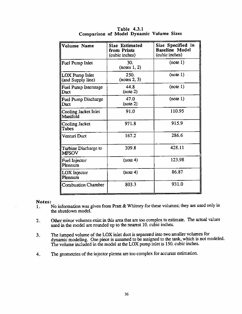
Notes:1.

.

.

.

Table 4.3.1

Comparison of Model Dynamic Volume Sizes

Volume Name Size Estimated Size Specified infrom Prints Baseline Model

(cubic inches) (cubic inches)

Fuel Pump Inlet 30. (note 1)(notes 1, 2)

LOX Pump Inlet 250. (note 1)(and Supply line) (notes 2, 3)

Fuel Pump Interstage 44.8 (note 1)Duct (note 2)

Fuel Pump Discharge 47.0 (note 1)Duct (note 2)

Cooling Jacket Inlet 91.0 110.95Manifold

Cooling Jacket 971.8 915.9Tubes

Venturi Duct 167.2 286.6

Turbine Discharge to 309.8 428.11MFSOV

Fuel Injector (note 4) 123.98Plennum

LOX Injector (note 4) 86.87Plennum

Combustion Chamber 803.3 931.0

No information was given from Pratt & Whitney for these volumes; they are used only inthe shutdown model.

Other minor volumes exist in this area that are too complex to estimate. The actual values

used in the model are rounded up to the nearest 10. cubic inches.

The lumped volume of the LOX inlet duct is separated into two smaller volumes fordynamic modeling. One piece is assumed to be assigned to the tank, which is not modeled.The volume included in the model at the LOX pump inlet is 150. cubic inches.

The geometries of the injector plenna are too complex for accurate estimation.

36

,<

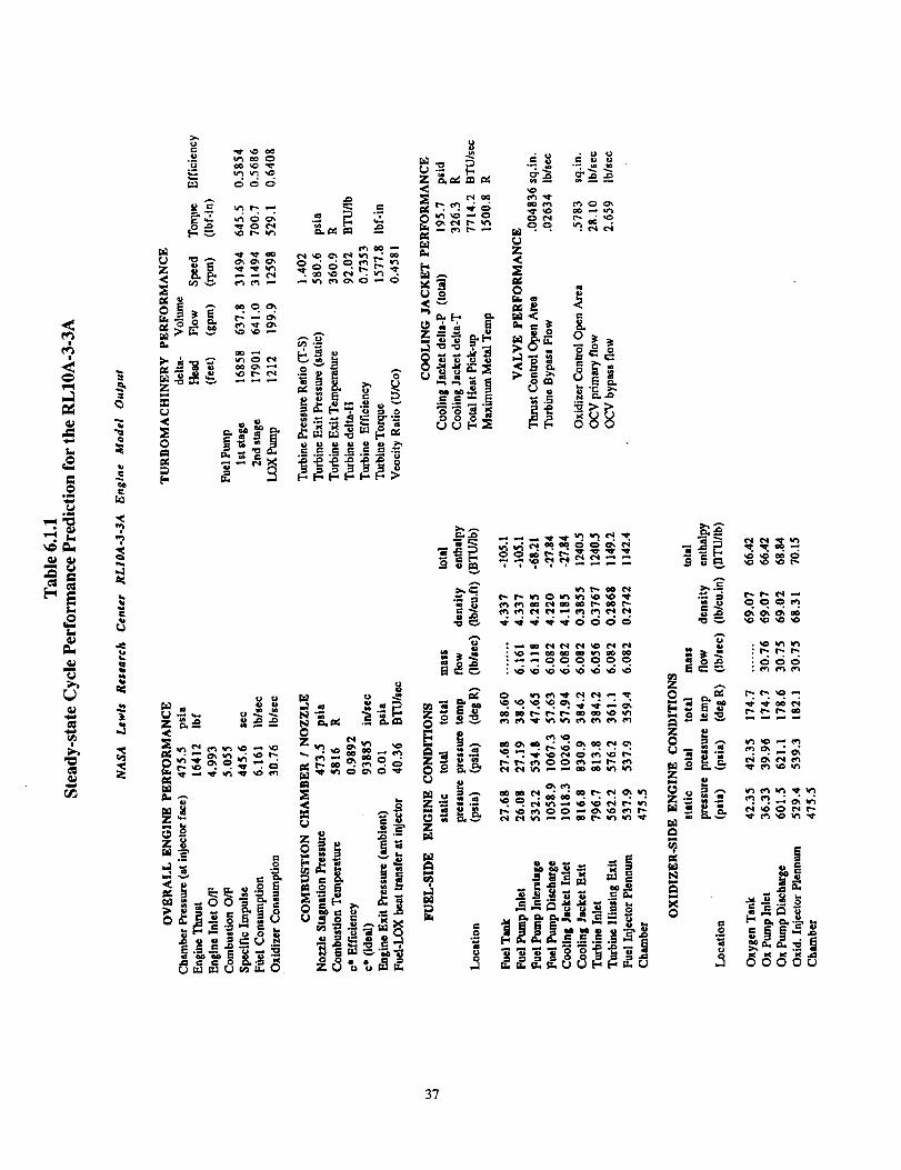
v=q

t.

c)omm

m

L.

2--

m

c:

1.1

_J

t.

____ _

.... .ooo°

6 ...... 6 =--

_ v% _elr'- t-- r'-

37

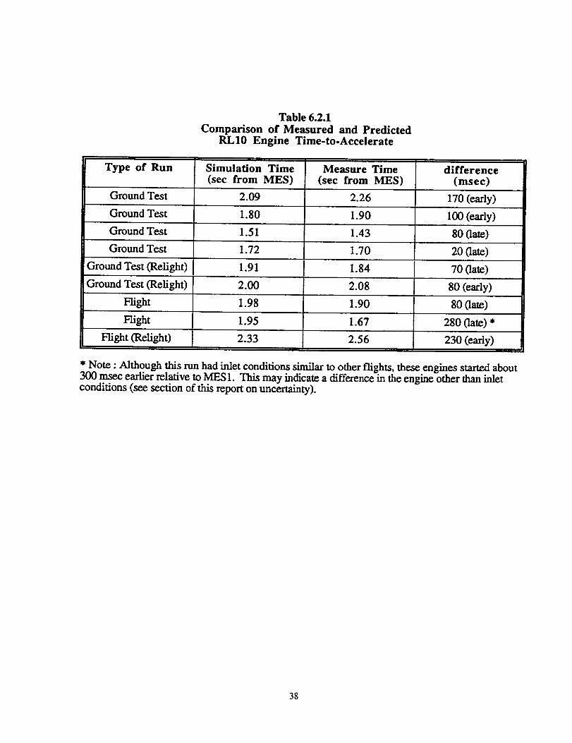
Type of Run

Ground Test

Ground Test

Ground Test

Ground Test

Table 6.2.1

Comparison of Measured and PredictedRL10 Engine Time-to-Accelerate

Simulation Time

(sec from MES)Measure Time

(sec from MES)difference

(msec)

20 (late)

Ground Test (Relight) 1.91 1.84 70 (late)

Ground Test (Relight) 2.00 2.08 80 (early)

Flight 1.98 1.90 80 (late)

Flight 1.95 1.67 280 (late) *

Flight (Religh0 2.33 2.56 230 (early)

2.09 2.26 170 (early)

1.80 1.90 100 (early)

1.51 1.43 80 (late)

1.72 1.70

* Note- Although this run had inlet conditions s'unilax to other flights, these engines started about300 rnsec earlier relative to MES 1. This may indicate a difference in the engine other than inletconditions (see section of this report on uncertainty).

38

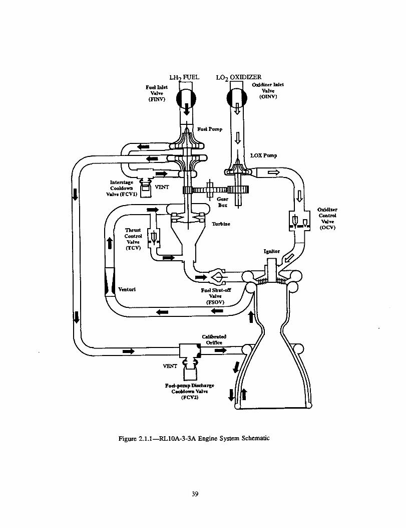
1

Fuel Inlet

Valve

(FI_

FUEL LO 2 OXIDIZEROxidizer Inlet

Valve

(OINV)

Fud Pump

lnterstageCooldowa

Valve (FCV1)

Thrust

Control

I Valvefrcv)

VENT

Turbine

LOX Pump

Ignitor

Valve

(Fsov)

Calibrated

Orifice

Fad-pump DischargeCooldown Valve

O_CV2)

OxidizerControl

Valve

(ocv)

Figure 2.1.1_RL10A-3-3A Engine System Schematic

39

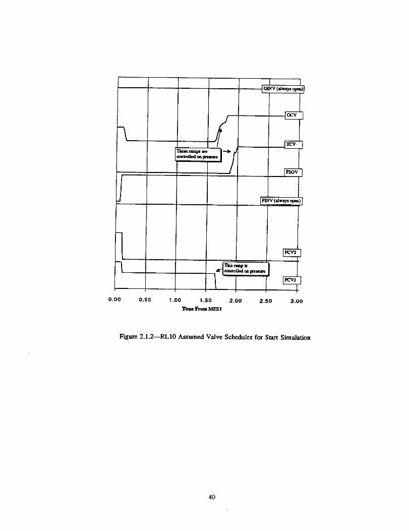
0.00 o.50

V (llwayi opm)_

1.00 1.50 2.00 2.50

'Time From MES 1

3.00

Figure 2.1.2_RLI0 Assumed Valve Schedules for Start Simulation

4O

.........-.........._

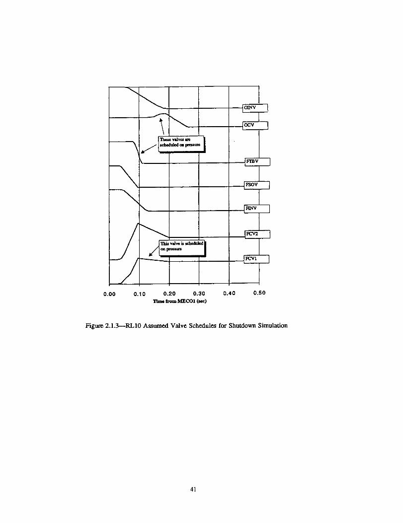
I

Figure 2.1.3--RL10 Assumed Valve Schedules for Shutdown Simulation

41

1ststage

Inducer

FUMPPUMPEXIT

2ridstageimp_

1st stagerarbine

Ink_ Nozzles

2rid stagemrb_ne

ExitGuideVanes

FUELPUMP

INLET

FUELTURBINE

EXIT

Gear Box

FUELFirst Stag, Second Stage TURBINEDischarge Inlet INLET

INTERSTAGEDUCT

Figure 2.2.1--Cross-Section of Fuel Pump and Turbine

42

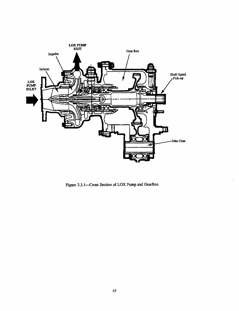
LOXPUMPGearBox

LOXPUMP

Inducer

Shaft Sp_d

Pick-up

Figure 2.3.I----Cross Section of LOX Pump and GearBox

43

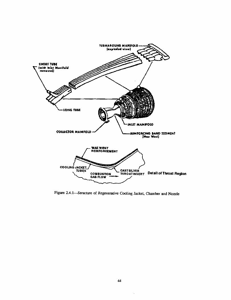
LONG TUllE

¢Ol.lLiaO| MANIFOLD

MANIFOLO

BAND $[GMENT[Me. W_st)

__ "MAE W EST +A

COOUN_

"IUBES -- _.. CASTSILVER" COMBUSTION "IHROATINSERT Detail of Throat Region

Figure 2.4.1--Structure of Regenerative Cooling Jacket, Chamber and Nozzle

44

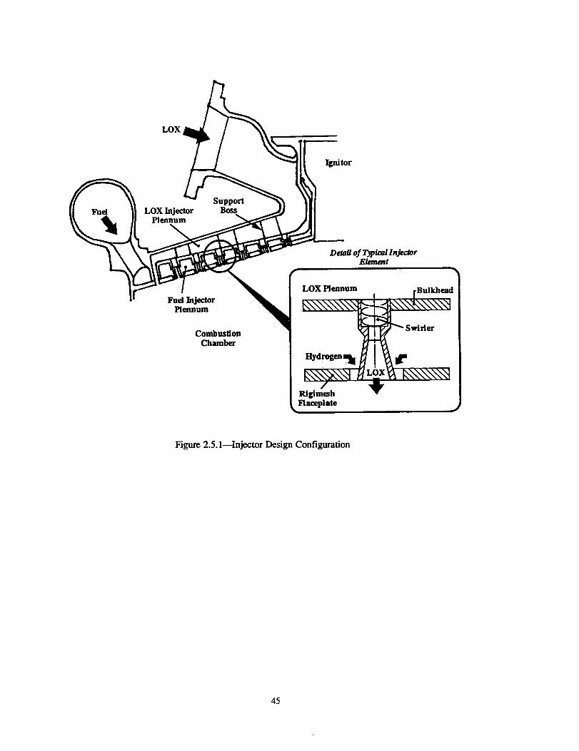
LOX

Igni tor

Fuel LOX InjectorPlennum

Fad InjectorPlennum

SupportBoss

CombustionChamber

Daail of Typical InjectorElement

LOX Plennum Bulkhead /

Figure 2.5.1---Injector Design Configuration

45

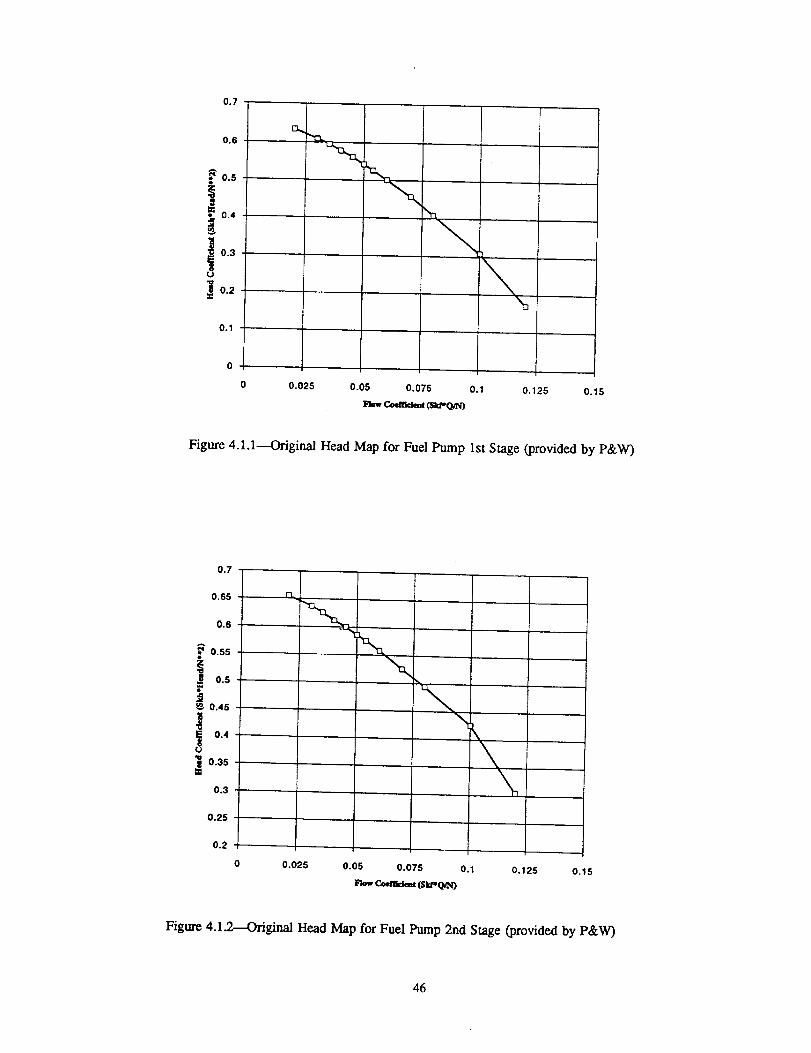
0.7

I0.6

0.5

0.4

0.3

"_ 0.2

0.1

0 0.025

\

0.05 0.075 0.1

l_w coenteke= (SlcPQ/N)

0,125 0.15

Figure 4.1.1---Original Head Map for Fuel Pump 1st Stage (provided by P&W)

0.7

0.65

0.6 "_.

o.ss

0.5

0.45

!'u

0.4

0.35

0.3

0.25

0.2

\

0 0.025 0.05 0.075 0.1

C-,_f_d_t (SlUr*O/N)

0.125 0.15

Figure 4.1.2---Original Head Map for Fuel Pump 2nd Stage (provided by P&W)

46

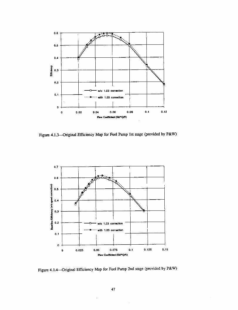
0.6

0.5

0.4

0.3

0.2

0.1

°db"O°°

w/o 1.03 correction

.... • .... with 1.03 correction

0 0.02 0.04 0.06 0.08 0.1

Flow Cod_kat (Sld-(_N)

0.12

Figure 4.1.3----Original Efficiency Map for Fuel Pump 1st stage (provided by P&W)

0.7

0.6

A

0.5

_0.4

!0.3

J 0.2im

0.1

/m

------o----w/o 1.03 correction

.... e---- with 1.03 correction

0 0.025 0.05 0.075 0.1

Flow Coemcleet (Skr, Q/N)

0.125 0.15

Figure 4.1.4--Original Efficiency Map for Fuel Pump 2nd stage (provided by P&W)

47

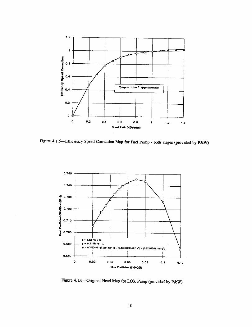
1.2

o

." 0.80o"oo

_. 0.6W

>.UCo"_ 0.4EW

1 '"

0.2

0

0

/

/

f

0.2 0.4 0.6 0.8 I 1.2 1.4

Speedl_llo O'_I/Nd_Ig_)

Figure 4.1.5--Efficiency Speed Correction Map for Fuel Pump - both stages (provided by P&W)

0.750

0.740

" 0.730

_ 0.720

•"_ 0.710

I

0.700

0.690

0.680

0.02 0.04 0.06 0.08 0.1

Row C._.flk_t (SI,PQtN)

0.12

Figure 4.1.6----Original Head Map for LOX Pump (provided by P&W)

48

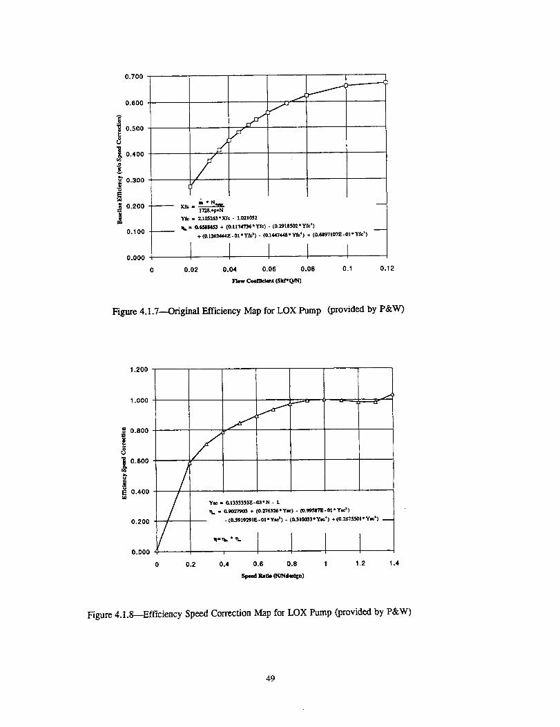
0.700

0.600

A

=='_ 0.500

_ 0.400

!_" O.3OO

Em

._ 0.200

0.100

0.000

/X.fc= _

1"/2&*p*Nyf¢ = 2.105263"X/0- L021052

qb= 0.6._8653 + (0.l174TJ6*Yf¢) - (0.2918502*Yfc=)+ (O.1262444E-OIeyf_) - (0.14474_'Yfc'i + (0.6_Y/IOTE-OI.Yfcs)

0.02 0.04 0.06 0.08 0.1 0.12

Coemckmt (Skt*O/N)

Figure 4.1.7--Original Efficiency Map for LOX Pump (provided by P&W)

1.200

1.000

o= 0.800

E_j

='_ 0.600

E 0.400r_

0.200

0.000

0

f

YI¢ = O.1333333E-03*N - L

. 0._0"Z_O_ + (0.Z7_'Ysc) - (0.99_ITE-OI'Ysc =)

- (0.591919=t= -01 *Ys_) - (O.310633"Ysc') + (0.2675501 *y_S)

I

0.2 0.4 0.6 0.8 1 1.2 1.4

Speed_=tb _des_)

Figure 4.1.8---Efficiency Speed Cor_fio, Map for LOX Pump (provided by P&W)

49

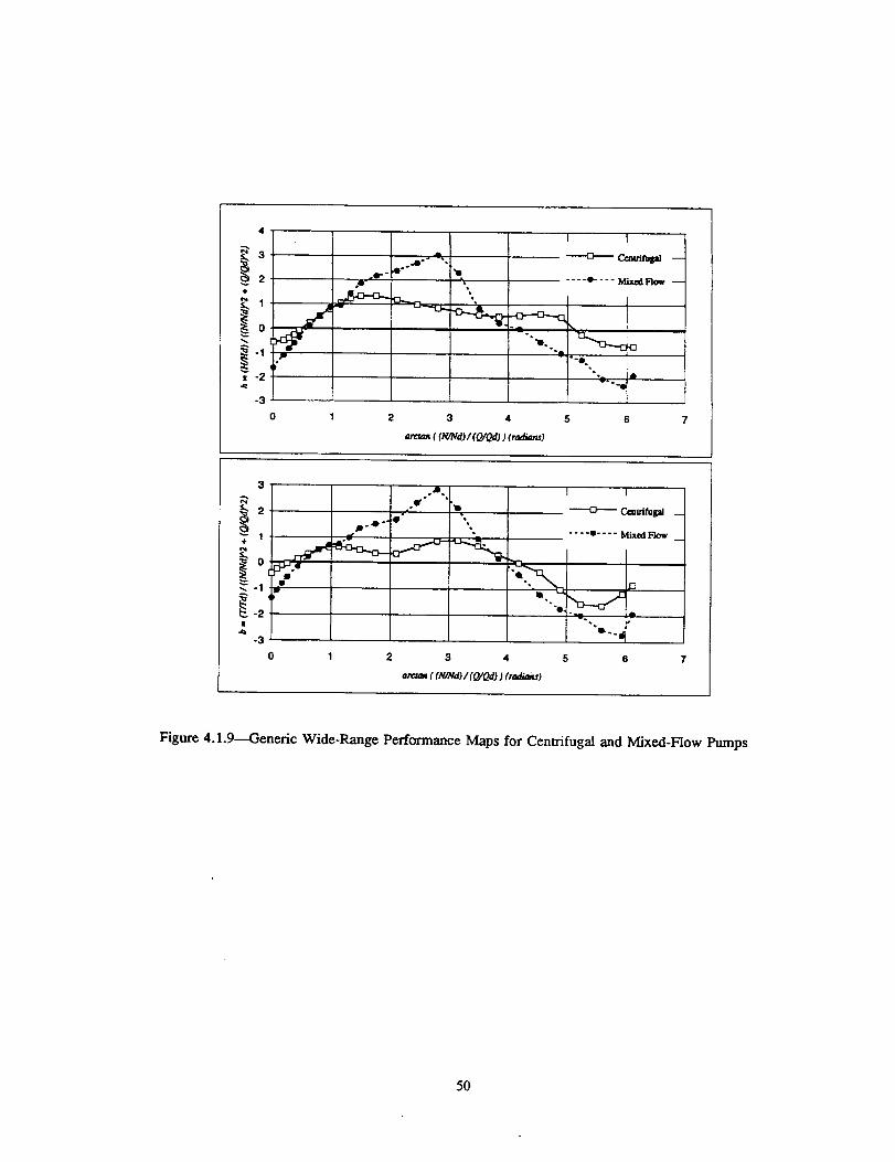
4 I I

_ 3 .11• "''e" . [3 C_i, ;_-a"2 .e-" _ .... e-- - - Mixed Plow --

""°-.. ° _c

I -2 "3.. I •

-3

0 1 2 3 4 5 6 7

arc_ ((N_d) / (QJQdl) (,adla_)

3

2 ,'f

D.4p.. 9 ° ",,

o _e

-2

-3

0

l I

.... • .... Mi.,,d FlOW

•"0_. -- L.

1 2 3 4 5 6 7

a_ ((N/Nd) / (Q/L_) ) (rad/_u)

Figure 4.1.9---Generic Wide-Range Performance Maps for Centrifugal and Mixed-Flow Pumps

50

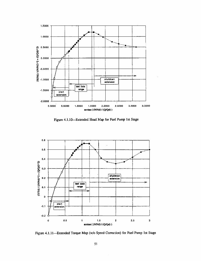
1.5000

1.0000

_" 0.5000<

_g"" 0.0000÷

;2-0.5ooo

_-1.0000

-1.5000

-2.0000

0.0000

)'°°',O-..°_J ._-v

0.5000 1.0000 1.5000 2.0000 2.5000 3.0000 3.5000

=rc_==((Z_qd) / (O/Qa))

Figure 4.1.10--Extended Head Map for Fuel Pump 1st Stage

0.6

0.5

0.4

0.3

-I-

< 0.2

-- 0.1

0

-0.1

-0.2

0 0.5 1 1.5 2 2.5 3

arclan ((N/Nd) I (QIQd))

Figure 4.1.11--Extended Torque Map (w/o Speed Correction) for Fuel Pump 1st Stage

51

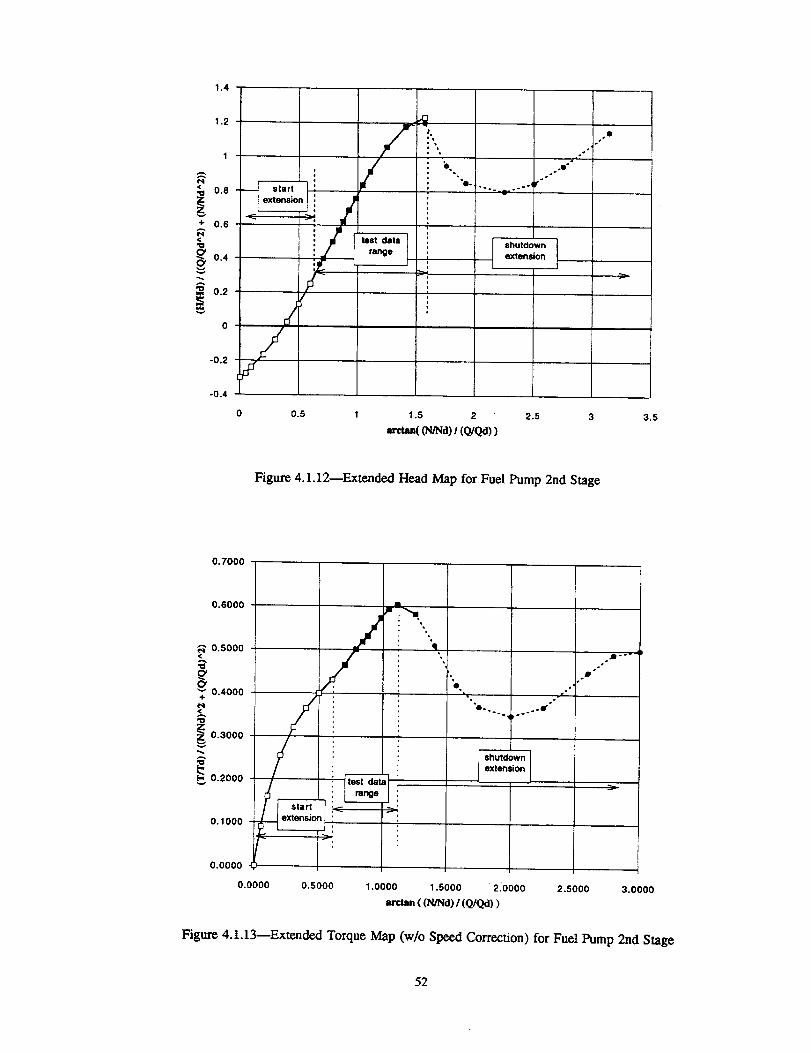
1.4

1.2

1

._ 0.8

+ 0.6

_ 0.4

_ 0.2

o

-0.2

-o.4

J/

S

/ ",ll

=

!

0- .. .°1*___ °o

v

shutdown

extension

°o

°4 °

°° °

f,"

.0°°

0.5 1 1.5 2 2.5 3

m'etaa((N/Nd) / (Q/Qd))

3.5

Figure 4.1.12---Extended Head Map for Fuel Pump 2nd Stage

0.7000

0.6000

0.5000<

g" 0.4000÷

N

"O

_ 0.3000

_ 0.2000

0.1000

0.0000

0.0000

.

om

o°

0.5000 1.0000 1.5000 2.0000

arctan((N/Nd)/(Q/Qd))

2.5000 3.0000

Figure 4.I.13---Extended Torque Map (w/o Speed Correction) for Fuel Pump 2rid Stage

52

1.2

0.8

<_ 0.6

"O

0.4+

PI

< 0.2

C_

_ 0

o0.2

-0.4

-0.6

-0.8

_ i J I_''''''1"''-

i

"°°.l

"1) ...........--e

0 0.5 1 _ 1.5 2 2.5

_-tan ((ht/Na)/ (Q/Qd))

3.5

Figure 4.1.14---Extended Head Map for LOX Pump

0.6

0.5

0.4

+

• 0.3

0.1

//,

"1

\Ii

lib°,

°.0 °

°.-""q r"

,0" °o-

oooo

.°,°

0 0.5 1 1.5 2

_ctan ((N/hid) I (QIQd))

2.5 3

Figure 4.1.15--Extended Torque Map (w/o Speed Correction) for LOX Pump

53

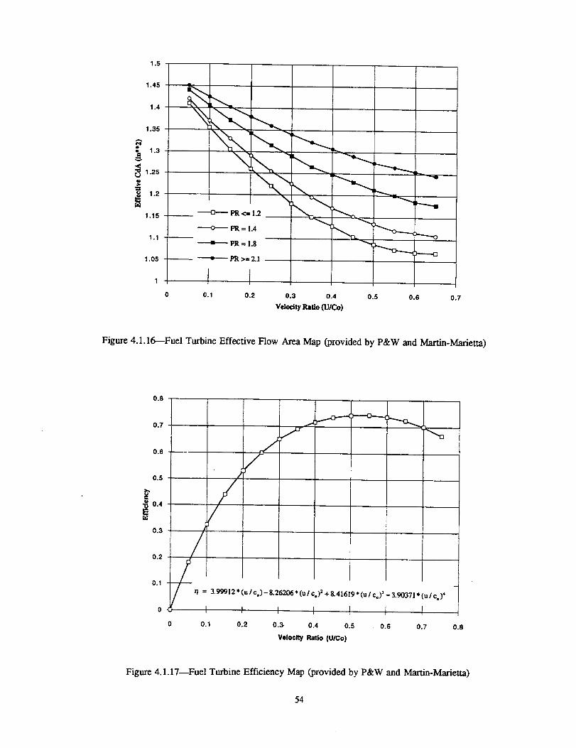
1.5

1.45

1.4

1.35

1.3m

_ 1.25

_ 1.2

1.15

1.1

1.05

1

--"_--'- PR >= 2.1

I I0._ 0.2 0.3 0.4 o.s o.s

VdodtyRaUo(U/Co)0.7

Figure 4.1.16---Fuel Turbine Effective Flow Area Map (provided by P&W and Martin-Marietta)

0.8

0.4E

07

0.5 /

0.3

I t0.1

3-99912 * (u / c,)- 8.26206" (u / Co) 2 + 8.41619" (u / C,) 3 - 3.90371' (u 1 C,) 4

0 I I I I t I

0 0.1 0.2 0.3, 0.4 0.5 0.6 0.7

Velocity Ratio (U/Co)

0.8

Figure 4.1.17-----Fuel Turbine Efficiency Map (provided by P&W and Martin-Marietta)

54

Section $

Chamber Axis _1_

Sectiom 1

Sectlam 2

S5

o

mid 'M_ West °

atBooked Stabiem-Ste_ Jdnts

Tube C.,ess_'tJon

3.2

3.1

3

2,9

2.8

:;'.7

Z.E

Z.5

2.4

2.3

2.2

|._mt- Tube C_',,--

(hmer mm)

!\

J

//

I

-1 -o.5 0 0..5

a

1

Figure 4.2.1---Configuration of Cooling Jacket and Model

55

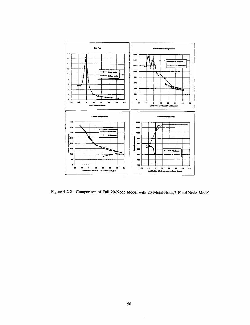
kk

I

./\°2a -Io o le N 14 4o so

_ooQ

14oo

_ _ L

14)0

N6

q4

H0

I

/li'_r4 Ilidd Tm

i_, I I I

\

.zo .lo o lo |o a@ 4o |4

IN

N

o

c,dm _lUn

\\

\

+-n -Io • +o _iii $o 4o IO

alll_ rll.,mm lr w,l_ Ik.l,41_ lrl Irll, mq_llkll I

Iloo

_IOSO

Iooo

11o4

t "

TSO

TO4

C,,eba _-_ pnemr_

J-to -l,n o 1o 20 lo 4o so

_lll l_ll_ .llld. g4.,p_l ,,rl 'Inl_ Omit)

Figure 4.2.2----Comparison of Full 20-Node Model with 20-Metal-Node/5-Fluid-Node Model

56

8500

_8000

7500

i7000

¢

6500

6000

12"

_J

...,.,_..----.,----"

f....-.x"

---o--------

T.d_vca (20 _k_)

H-dive. (20.aod_)

I I

4.5 4.75 5 5.25 5.5 5.75

MJxtare Ratio

Figure 4.2.3---Comparison of Enthalpy-Driven and Temperature-Driven Potential Predictions

20

18

16

14A

lO

8

6

-20

I

1

II

-10 0 10 20 30

/,Jdal Locatkm - Node Mldpobats _es _-t T'aroa0

4O 5O

Figure 4.2.4---Predicted Heat Flux Distribution

57

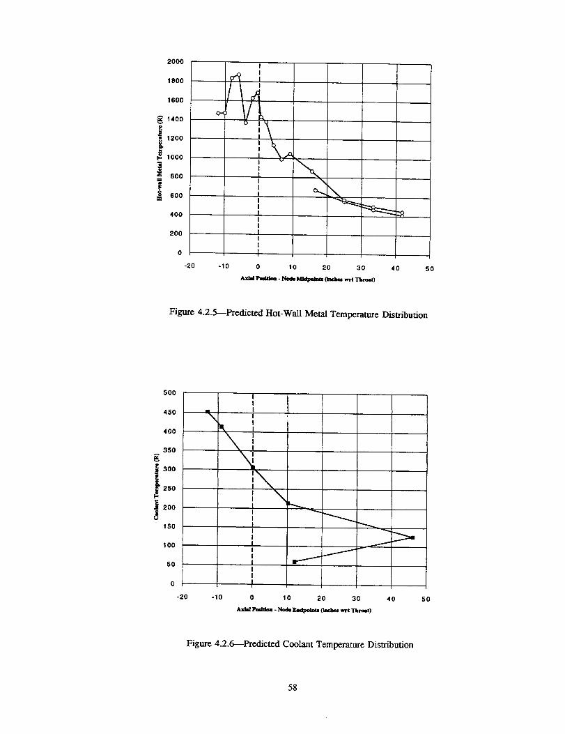
2OO0

1800

1600

1400

1200

lOOO

800

6O0

400

200

o

-20 40 5O

Figure 4.2.5---Predicted Hot-Wall Metal Temperature Distribution

500

450

400

350

300

250

¢:

200

150

I O0

5O

0

-20

\

-10

IIIII

i\J _I _

I

' III

0 10 20 30 40

]_dCba - Node]g_lpelma (J_l_ _ Tm_t)

5O

Figure 4.2.6---Predicted Coolant Temperature Distribution

58

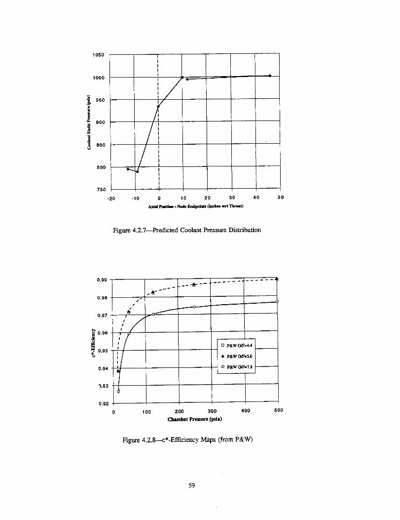
m

1050

1000

950

900

850

800

750

-20

IIIII

//"III

IIII

-lO 0 10 20 30

,_tlai Podel_. Ns_ _ (_1_ wrt Tbroa0

40 50

Figure 4.2.7----_edicted Coolant Pressure Distribution

0.99

0.98

0.97

0.96¢

E_, o.gs"o

0.94

'3.93

0.92

d

.._...--o------

/

/

I

I

[3 P&W O/F=4A

• P&W O/F-_5.0

O p&w O/F_7.8

100 200 300

Chamber Pressure (psla)

400 5OO

Figure 4.2.8---c*-Efficiency Maps (from P&W)

59

450

00

--_ 350 i///,i I

_300¢=,,

r_q

250 .,,,

::::::**

200 =;,

JII ...... I

°°°"

_ "I'DIE/ODE. FC=I5 psia

TDIOODE. PC=500 psia

.... • .... P&W dalaat PC=i5

.... • .... P&W damat PC=500

f2 4 6

Mixture Ratio (OR;')

o.

I

8 10

Figure 4.2.9--TDK/ODE Predictions of RL10A-3-3A Actual Isp, compared to data provided by P&W

0.96

I_ = (_)oDB* _cf *TI=*

.°

#°

0.94 3"

o S3. o.,2

o°° s A

i o., o-.-2"

i_ 0.88

0.86 i

0.84

.-°-°'_

.... EP--- O/F=I

0_=4

.... C---- O/F=6

----.l.--- O/F= 10

----_--- O/F = 20

---.......k_ O/F = 50

I0 100 200 300 400 500

C_=,,=_We=u't_)

Figure 4.2.10---TDK Predictions of RL 10A-3-3A Thrust-Coefficient Efficiency

60

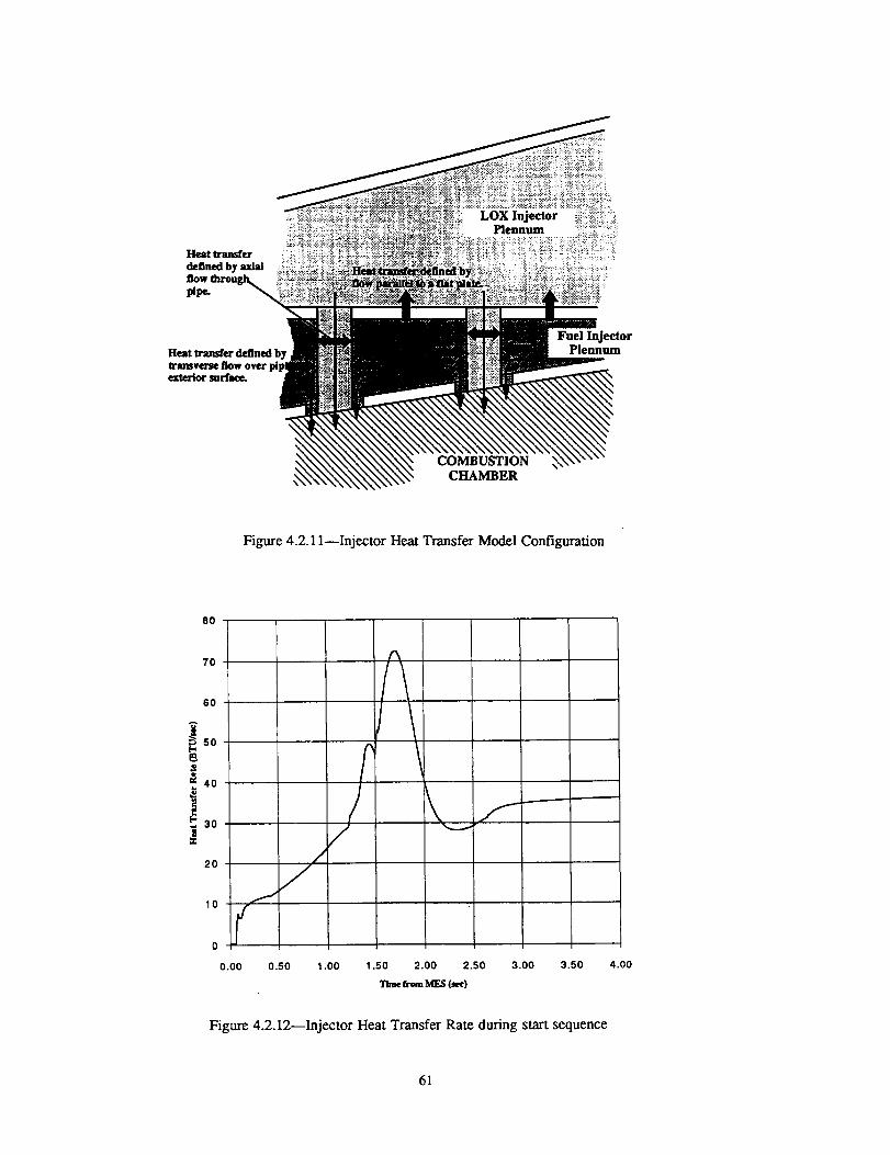
Fuel InjectorPiennum

COMBUSTION

CHAMBER

Figure 4.2.1 I--Injector Heat Transfer Model Configuration

8O

70

6O

so

40

308

Io (f0

0.oo 0.50 1.0o 1.5o 2.00 2.50 3.00 3.50

"l'lme Item MES (s_)

4.00

Figure 4.2.12--Injector Heat Transfer Rate during start sequence

61

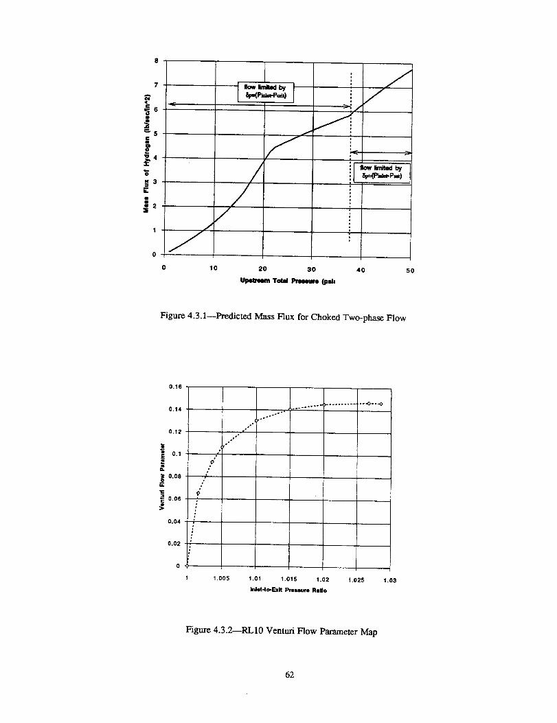
7

F

='5.=g_4

x3:l

,-r

==2:B

>!/

J

rNov+ _,,,_<I by8l:,-(Pi=_=..Pcd¢

++

'[ llow limited by8p=(Pak,-P--*)

ai

o 10 20 30

UpetrmmTam Pmmre Cn_40 5O

Figure 4.3.1--Predicted Mass Flux for Choked Two-phase Flow

0,16

0.14

0+12

0.1

t.• 0,08o

c...

0.06

0.04

0.02

r °°°

ow

,o

l

°+

|+

i

1 1.005

J....................++_.o•°o-'°

1.01 1.015 1.02

Inlet-to-Exit Presm_re Rdo

1.025 1.03

Figure 4.3.2--RL10 Venturi Flow Parameter Map

62

])

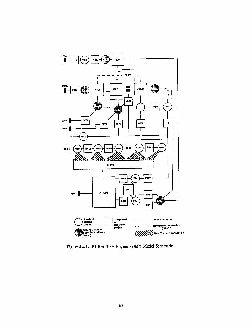
Os._, [--]_.oo..Volumeundue t I Resistance

'td. VoL Module Module

( only In ShutdownModel}

Flulcl Connection

Mechanical Connection

( Sh,n )

_\\\\'_..,,..,.cono.,,oo

Figure 4.4.1--RL10A-3-3A Engine System Model Schematic

63

-£

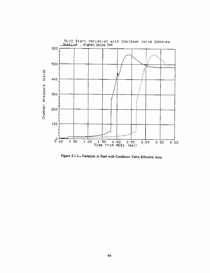
ID.

f...

B3

rl

(_

E

r-U

BOO

5OO

400

300

200

RLiO Start variation with Cooldown Valve CO*AreaBase 1 i ne __Hi_q_hef__V_lye_ CclA

iO0 I '_l

00. ._.___r-_-------_------_--'_-. ...........O0 O. 50 I .00 1.50 2.00 2.50

T:Jme from MESI (sec)

IIIII.

i I

1I

I

/

iI

I

I

II

I

II

1

3.00 3.50 4.00

Figure 5.1.1--Variation in Start with Cooldown Valve Effective Area

64

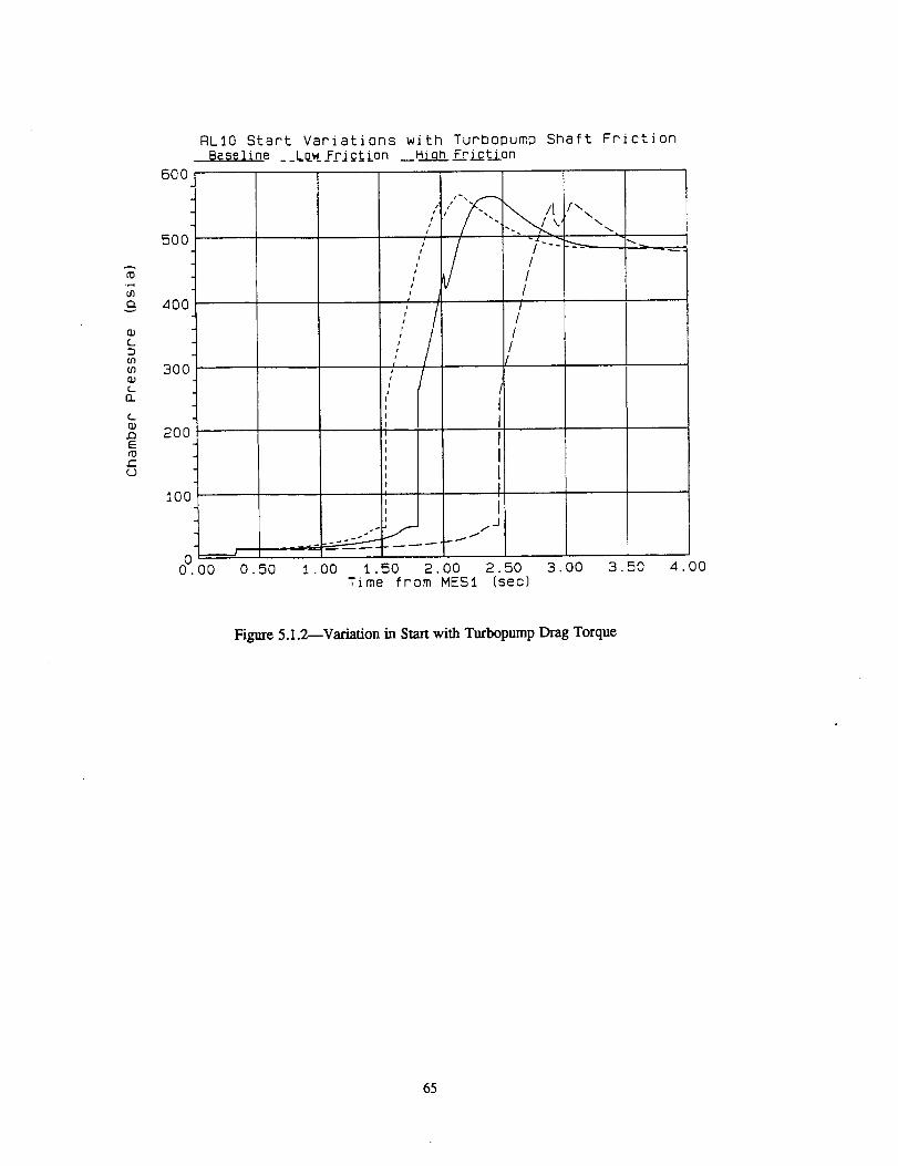
CI

(_D

(n

(_£L

(_

nE_D

6OO

500

400

30O

200

RL_0 Start Variations with Turbopumo Shaft Friction@¢se]ine __LEw_ZfJ_;tion _Hiqh F__r_ction

I00

00.00

/ /

/ /

, // /

/ !

.' i/

/' I (

i!

0.50 i .00 1.50 2.00 2.50Time from MES1 (sec)

,f\\\

3.00 3.50 4.00

Figure 5.1.2--Variation in Start with Turbopump Drag Torque

65

r_v

GD

In

rl

Q;/3E

c-

B00

500

400

300

200

iO0

-.-J;

0v O0 0.50

gLiO Start Variation with OCV Actuation Pressures

Baseline (80 psid) ___p_e_n_s__J;__q_psid __ODe_Q.SjLtSO_psid

J

I,I!

I .00 i .50 2.00 2.50 3.00Time from MESI (sec)

3.50 4.00

Figure 5.2.1--Variation in Start with OCV Actuation Pressure

66

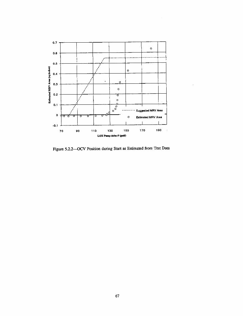
.,J

!.<

0.7

0.6

0.5

0.4

0.3

0.2

0.1

°l°-0.1

7O

w•a•

o./

t"

_J

/o

.edw

0 o 0 0

,---a•

0

0

0

00

00

_Cm

0

90 110 130

i

......... Suggested MRVArea

o EsSmatedMRV Area

i I I

150 170 190

Lox Plump dtJb-P (_id)

Figure 5.2.2---OCV Position during Start as Estimated from Test Data

67

c)

C_

D

83

O_

O_

[3_

t_

Q)

r_

E

¢0

r-

(.3

600

50O

RLiO Start Variation w_th In_tlal Chamber Netal TempBaseI_ne(@4OR) __Lo_w_Tem__.[_5OR)

zOO

3O0

2O0

_00

0 __.__j-- i0.00 0.5O

I I

I

I

I

I

I

I

II

1

t tI

i t

t_

I/

I'

I

it

/i

s

?'

1.5O 2.00 2.5OT_me from NES (sec)

3.00 3.50 4.00

Figure 5.3.1--Variation in Start with Initial Jacket Metal Temperature

68

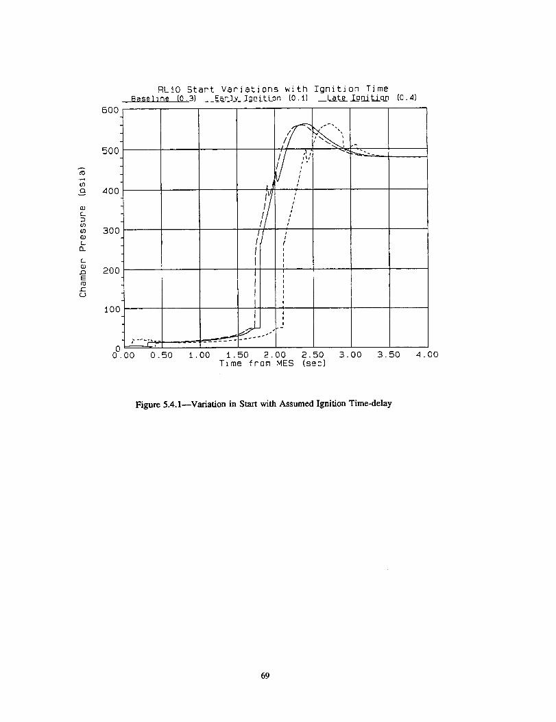
fO

gQ

CO[_

01O3(D(_0_

mE

C_)

600

500

4OO

3OO

2OO

iO0

00.00

RLIO Start Variations with Ignition TimeBaseline (0.3) ___%r_]_V__Ig__tt_Lon(0.I) _La_t_e_Ion__it_io_n(0.4)

J /

a

ili ;iIIi

I- I

I :!I

0.50 1.00 1.50 2.00 2.50Time from MES (sec)

if

3.OO 3.5O 4.OO

Figure 5.4.1--Variation in Start with Assumed Ignition Time-delay

69

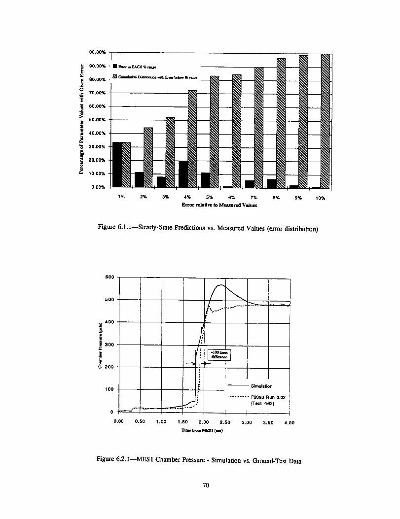
100.00% I

80.00% [] C=m=l=iv¢D_b_Joa _i_ Em=rb=low% ,_1==

>

_, 70.00%

60.00%:=

_, 5o.oo%

40.00%

30.00%

20.00%

=" 10.00%

0.00%

1% 2% 3% 4% 5% 6% 7% 8% 9% 10%

Error relative to Measured Values

Figure 6.1.1--Steady-State Predictions vs. Measured Values (error distribution)

60O

500

400

E

,_ 300

J|

200

100

1 .o0 1.50 2.00

Simulation

......... P2093 Run 3.02

(Test 463)

I i i

2.50 3.00 3.50 4.00

Tlhmefrom MI_! (_)

Figure 6.2.1--MES 1 Chamber Pressure - Simulation vs. Ground-Test Data

7O

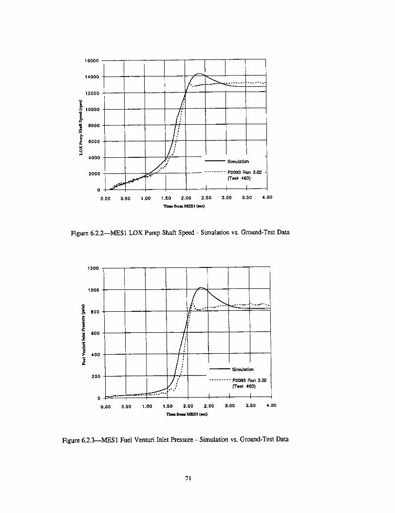
16000

14000

12000

!k 10000

i 8000

6000

4000

2000

0

0.00

f

/..:

0.50 1.00 1.50 2.00

....... . .°..°°...

Simulation

• - ........ P2093 Run 3,02

(Test 463)

I I I

2.50 3.00 3.50 4.00

Time from M]_ | (sec)

Figure 6.2.2--MES1 LOX Pump Shaft Speed - Simulation vs. Ground-Test Data

1200

1000

m

800

i600

]

400I

200

S

4.00

Simulation

......... P2093 Run 3.02

(Test 463)

0.00 0.50 1.00 1.50 2.00 2.50 3.00 3.50

fro,, MOKSl(_)

Figure 6.2.3---MES 1 Fuel Venturi Inlet Pressure - Simulation vs. Ground-Test Data

71

800

700

6OO

i

j 500

_400

_" 300

J 200

100

0

0.00 0.50

=

1.00

d I_- Simulation

......... P2093 Run 3.02

(Test 463)

I I I

3.00 3.50 4.001.50 2.00 2.50

Tin= from MF..Sl (see)

Figure 6.2.4---MES 1 LOX Pump Discharge Pressure - Simulation vs. Ground-Test Data

800

oo6OO

E 500 ""

i400 . ""

300 /"

2OO

100

0

0.00 0.50 1.00

"-_---i ....

Simulation

......... P2093 Run 3.02

(Test463)I I I

1.50 2.00 2.50 3.00 3.50 4.00

Time from bllES1 (_¢)

Figure 6.2.5--MES l Turbine Inlet Temperature - Simulation vs. Ground-Test Data

72

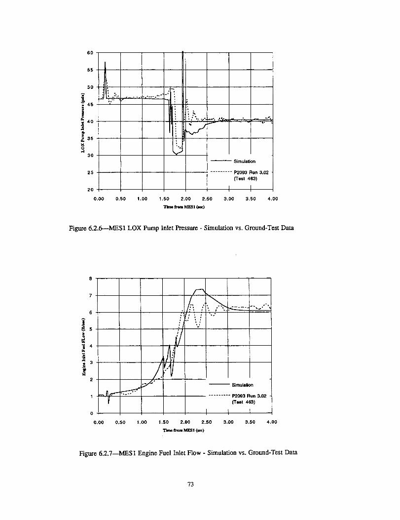
t

]t,=X0

6O

55 1

50: .

45

40

35

3O

25

20

0.00

i

i

Simulation

......... P2093 Run 3.02

(Test 463)

I I

,ho

0.50 1.00 1.50 2.00 2.50 3.00 3.50 4.00

Time from MESl (_:)

Figure 6.2.6--MES1 LOX Pump Inlet Pressure - Simulation vs. Ground-Test Data

6A

i4c,..w

__3

2

/.....•"l J i

• q*

Ji •i •

SimulationIt

1 -":_-_'_"" """ - ........ P2093 Run 3.02

f (Test 463)

0 i I I

0.00 0.50 1.00 1.50 2.00 2.50 3.00 3.50 4.00

TIn_ from MESl (_.c)

Figure 6.2.7--MES 1 Engine Fuel Inlet Flow - Simulation vs. Ground-Test Data

73

40 •

35

3O

25==

20o

10

0

I i,/"_\

I

=

i

M

j.,J../

Simulation

......... P2093 Run 3.02

(Test 463) __

0.00 0.50 1.00 1.50 2.00 2.50 3.00 3.50 4.00

TI=_ h-ore MESl (Kc)

Figure 6.2.8---MES 1 Engine LOX Inlet Flow - Simulation vs. Ground-Test Data

600 I

I500 ,

i

400

i

300

!200

!i 0

i

I D: w

iD

= ,

i

-= __ o--

0.00 0.50 1.00 1.50 2.00

I

- I00=_cdg"f¢=_¢¢

Simulation

......... P2093 Run 7.01

(Test 467)

I I 12.50 3.00 3.50 4.00

fro= MES2 (=e¢)

Figure 6.2.9--MES2 Chamber Pressure during Start - Simulation vs. Ground-Test Data

74

6OO

500

al•m 400m.

,,,1

_300

i.= 200¢J

lOO

-- Simulation Results

......... AC-72 Flight Data

i

i

d

i

- tO0 m_diffcr=w.,c

0.000 0.500 1.000 1.500 2.000 2.500 3.000

Time from MES1 Signal (see)

Figure 6.2.10--MES1 Chamber Pressure - Simulation vs. Centaur Flight Data

16000

14000

_, 12000

10000

E

0

8000

6000

4000

2000

0

0.000

-- Simulation re.suits

......... AC-72 Flight Data

.2/

0.500 1.000 1.500 2.000 2.500 3.000

Time fromMES Signal(see)

Figure 6.2.11--MES 1 LOX Pump Shaft Speed - Simulation vs. Centaur Flight Data

75

800

700

600

500

400

z=.

300

200

100

o

.°

.-

Simulat_n

......... AC-72 Flight Data

0.00 0.50 1.00 1.50 2.00 2.50 3.00

Time tr_m M]ESI (=e¢)

Figure 6.2.12--MES 1 Turbine Inlet Temperature - Simulation vs. Centaur Flight Data

600

500

400

E

j 300

!200

100

I 1 I

Simulation

......... AC-74 Flight Data --

(Engine Cl)

I

L_

I

_2""i

dln'a'_¢e !

0.00 0.50 1.00 1.50 2.00 2.50 3.00 3.50 4.00

"rim= tin= M]ESZ(_¢)

Figure 6.2.13--MES2 Chamber Pressure - Simulation vs. Centaur Flight Data

76

==

m

8

i

1900

1700

1500

1300

900 j7O0

5O0

0.00 0.50 1.00 1.50 2.00 2.50 3.00 3.50 4.00

TIz_fromM]gSl(see)

Figure 6.2.14--Predicted Maximum Metal Temperature during Start Transient

250

(OCV is commanded to open at dP OP indicated, but valve is

200

_15o

i

1oo0

5o

/

_,; ......... Baseline (d? OP--80-

._ 124'_d)

.J__ -- (d.PO1)=-150-200I_id)

0

0.00 0.50 1.00 1.50 2.00 2.50 3.00 3.50 4.00

Time from M3_l (_)

Figure 6.2.15--Predicted Ignitor GOX Supply delta-P during Start (variation with OCV opening pressure)

77

5OO

450

400

35O

3300

9'

250

200

150

100

5O

i

J

"I

0 0.2 0.4 0.6

from MECOI (=¢)

I ISimulation

......... P2093 Run 8.01

('Test 468)

0.8 1

Figure 6.3.1--MECO1 Chamber Pressure - Simulation vs. Ground-Test Data

13000

12000

11000

10000

9000

8000LE

70000

6000

5000

4000

I ISimulation

......... 1>2093 Run 8.01

('Test 468)

I

....... ..°.

0 0.2 0.4 0.6

Time from MECO1 (see)

0.8 1

Figure 6.3.2--MECO1 LOX Pump Shaft Speed - Simulation vs. Ground-Test Data

78

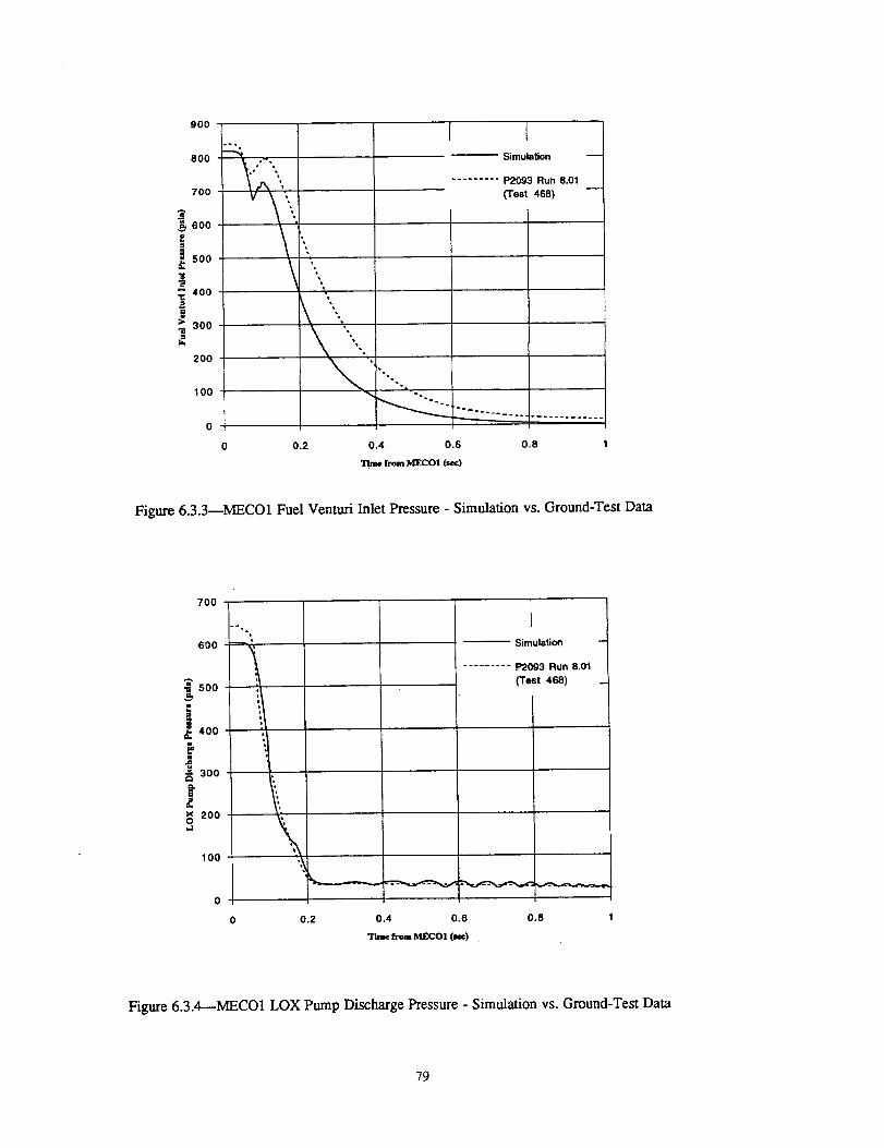
9OO

8OO

700

a

_, 600P

i 500

1

M•t: 400

;: 300

2OO

IO0

0

Simulation

......... P2093 Run 8.01

(Test 468)

0 0.2 0.4 0.6 0.8 1

frem MBECOI (see)

Figure 6.3.3--MECO1 Fuel Venturi Inlet Pressure - Simulation vs. Ground-Test Data

700

600

5O0

1ill 400,v

300

X 2000

100

°=

.!

Simulation

......... P2093 Run 8.01

(Test 468)

0 0.2 0.4 0.6 0.8 1

Time/tom tdggCOl (_¢)

Figure 6.3.4---MECO1 LOX Pump Discharge Pressure - Simulation vs. Ground-Test Data

79

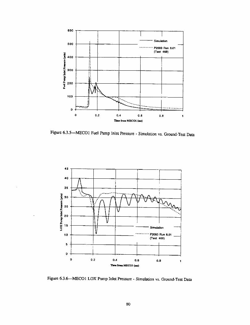
600

500

.i4oo

300

200

100

D

,o

I,

\

Simulation

......... P2093 Run 8.01

(Test 468)

0 0.2 0.4 0.6 0.8 1

"llme from blF_,COI(_ec)

Figure 6.3.5--MECO1 Fuel Pump Inlet Pressure - Simulation vs. Ground-Test Data

II

1¢

t

xQ,.J

45

40

35

30

25

20

15

10

5

0

I

/l

......--.

°e "° /_,

VV

Simulation

......... P2093 Run 8.01

(Test 468)

0 0.2 0.4 0.6

"lime from MECOI (see)

0.8 1

Figure 6.3.6---MECO 1 LOX Pump Inlet Pressure - Simulation vs. Ground-Test Data

80

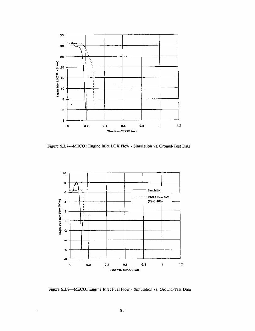
35

25 •I

_20 ",,

_ ,,i

_ 150

ea

_ 10i, !

,o

°0 r

-5

0 0.2 0.4 0.6 0.8 1 1.2

Tlme from M]gCOt (_)

Figure 6.3.7--MECO1 Engine Inlet LOX Flow - Simulation vs. Ground-Test Data

10

4

2

1 o

9-2m

-4

-6

-8

Simulation

......... P2093 Run 8.01

('Test 468)

0 0.2 0.4 0.6 0.8 1 1.2

TI_ CramMSCOI (mc)

Figure 6.3.8---MECO1 Engine Inlet Fuel Flow - Simulation vs. Ground-Test Data

81

500

450

400

350i=1

300

250

200,¢1_J

15o

100

5O

o

:=i

•1

0 -"

Simulation

......... AC-72 Flight Data

0 02 0.4 0.6 0.8 1

'llme from MIECOI (see)

Figure 6.3.9mMECO1 Chamber Pressure - Simulation vs. Centaur Flight Data

13000

12000

11000

10000

I 9000

8000

t 7000

M

6000

5000

400O

3000

% I I

Simulalion

_ Data averaged over.05 sac

......... Actual Right Data

oo..ioooo °o[,, ,..,_ _,_

;; ,; • ;,'v,H, I-'-" :: :: :.::i

: I:I: IT :"1;:"• ii e• i_

'Di j!

li: i_llii,.'i!;

0 0.2 0.4 0.6 0.8 1

'llme _ ME,COl (_¢)

Figure 6.3.10--MECO1 LOX Pump Shaft Speed - Simulation vs. Centaur Flight Data

82

m

Ba-

"d

"C

900

800

7OO

600

500

400

300

200

tO0

0

0

!::" ':,

11

i

I l-- Simulation

......... AC-72 Flight Data

I

_ _ . ° "'-...o__ --..., ._._

0.2 0.4 0,6 0.8 1

Figure 6.3.11--MECO1 Fuel Venturi Inlet Pressure - Simulation vs. Centaur Flight Data

700

600

I

500

400

300

t

200

100

t

I ISimulation

......... AC-72 Right Data

I

0 0.2 0.4 0.6 0.B 1

TI_ from MECOI (see)

Figure 6.3.12--MECO1 LOX Pump Discharge Pressure - Simulation vs. Centaur Flight Data

83

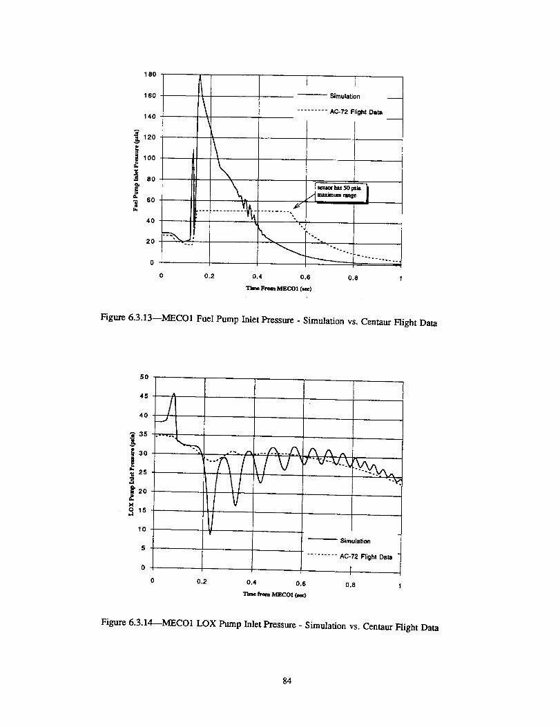
180

160

140

,_120

._ 100

e_

•a so¢1.

|"i sor_

4O

2O

I

-°.,

J

\

0 0.2

I I

Simulation

......... AC-72 Flight Data

E

_ bassopm Ij maxim nm_

_.o..o .....

0.4 0.6 0.8

Time From MECOZ (leo)t

Figure 6.3.13--MECO1 Fuel Pump Inlet Pressure - Simulation vs. Centaur Flight Data

50

4O

35 .- ....

_30 -°'- /'_

/E 20

V0 15,,.1

10

5

0

0 0.2

..../:k--/_'_A A ,.,

Simulation

......... AC-72 Right Data

I0.4 0.6 0.8

Time from MIBCO1 (sec)

Figure 6.3.14---MECO1 LOX Pump Inlet Pressure - Simulation vs. Centaur Flight Data

84

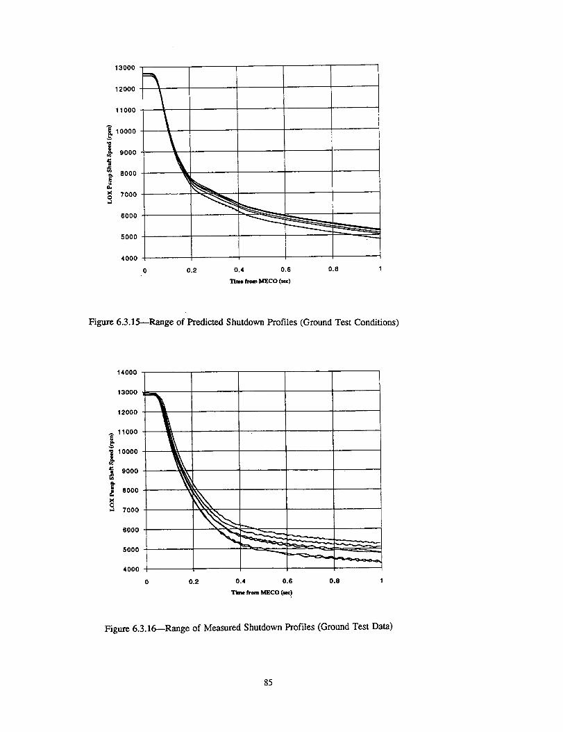
IIIIZ11000 t_

L \

i 9000 _k

0 0.2 0.4 0.6 0.8 1

from M]ECO (==¢)

Figure 6.3.15---Range of Predicted Shutdown Profiles (Ground Test Conditions)

14000

13000

12000

11000L

10000

9000

teooo

@7000

6000

5ooo

4000

' _ _-_"_'_ "_-_t,_

0 0.2 0.4 0.6 0.8 1

a'_ ,_ MECO(,_,)

Figure 6.3.16---Range of Measured Shutdown Profiles (Ground Test Data)

85

APPENDIX A

RL10A-3-3A Engine System Model for ROCETS

The RL10A-3-3A rocket engine was simulated using the Rocket Engine Transient Simulator

(ROCETS) program (Reference A1). The model of the RL10 is comprised of four elements: 1) thesystem configuration file(s), 2) the run input file and guess file, 3) the component modelsubroutines, and 4) the utility and solver subroutines. This utility and solver routines are the same

for any ROCETS model and are not discussed further in this report.

The system configuration file contains information about what components are included, whatsubroutine is used to model them, and how they are connected. Two models of the RL10 exist;one for the start transient and steady-state performance, the other for the shutdown transient. Both

models are represented schematically in Figure A.1. The ROCETS preprocessor software (whichmust be run before compiling and linking the simulation) uses the configuration input files to writeFORTRAN code for the system simulation. Equations in the input file are written as expressionsin the FORTRAN code. Component 'Modules' and 'Property Package' blocks are converted into

calls to the appropriate subroutines. The preprocessor uses information stored in the headers ofeach component subroutine to write its call list in the FORTRAN program. The configurationinput files also contain information about state substitutions and additional algebraic balances.

The run input files contain execution instructions for each simulation run. These fries containdescriptions of model boundary conditions (such as tank pressures and temperatures), initialconditions (such as jacket metal temperature), and schedules for ignition and valve movement. Therun input files also contain a great deal of instructions governing the convergence of the modelsolver, this information must be especially detailed for the transient simulations, which oftenencounter conditions where numerical convergence may be difficult (zero flow, zero rotation,sudden valve movements or ignition, etc.). The run input files also define the type of run to be

performed (steady-state or transient). During execution, a guess subroutine is called which sets theinitial values of state variables in the model. The guess file can contain simple value assignments

or procedural code (to set initial enthalpy based on user input temperatures, for example). A single

guess file is used for all RL10 simulations (start, steady-state, shutdown).

Each component in the engine system is modeled by a FORTRAN subroutine. Severalcomponents, the pumps for example, may use the same basic routine, but with different designinformation (values or maps).

To obtain a copy of the RL10A-3-3A model input files and component subroutines, the interestedreader should contact Mr. Joseph Hemminger at the NASA Lewis Research Center. To obtain a

copy of the ROCETS program (utility and solver software), please contact Mr. David Seymour atthe NASA Marshall Space Center.

A1.

References

Pratt & Whitney Government Engines, Design Report for RLI OA-3-3A Rocket Engine,

(NASA Contract NAS3-22339, Pratt & Whitney Report No. FR-15876), January 1982.

87

-7

/

Q Standard I_ Component F]uld ConnectlonVolume orModue Resistance

Mechanical Connection

L_--_Rtd. VoL Module Module ( Shaft )

_-_,_ (Ohly ,n Shutdown .__Model} Heat Trar_fer ConnecUon

88

APPENDIX B

Component Modeling of RL10 Fuel and Oxidizer Pumps

This appendix to the RL10A-3-3A Modeling Project Final Report describes efforts to predict theperformance of the RL10 fuel and oxidizer pump using component analysis programs available tothe NASA Lewis Research Center Space Propulsion Technology Division (SPTD). Cross-

sectional views of the pumps are shown in Figures B 1 and B2.

B 1. Analytic Tools usedThe SPTD has been working to develop turbomachinery design and off-design programs forseveral years. Since the RL10 design geometry was already set, only the off-design performancecodes were used in this projecL The programs utilized were PUMPA (Reference B 1) and LSISO

(Reference B2). These codes are one-dimensional mean-line codes, which means that two andthree dimensional effects are either averaged across the flow-area, or corrected for using, empirical

factors. A third program was written to predict low-speed pump performance from a given design

point using a method described in Reference B3.

The PUMPA analysis code uses a combination of theoretical calculations and empirical correctionfactors. Velocity triangles are used to determine the theoretical head rise though the impeller. Thecorresponding discharge pressure is then corrected using empirical relations for design efficiency,variations in efficiency with speed, and two-dimensional effects at the impeller exit (expressed as

an empirical function of geometry, flow and s.p_e,d!. Likewise, diff .u:_r,,andvolu_losses oa_enadetermined based on flow velocities, lne empmcat correcuons are a_sttttea zrom test uata unumber of different types of turbopumps _ including the RL10 turbopump). The correctionscan therefor be considered generic empiricisms which may be applied to any problem, and are not

tailored for the RL10 alone.

LSISO (Loss Isolation program) appears to involve fewer explicit empirical correlations thanPUMPA, but data contained in the program has almost certainly been tailored to better match testcases in the past as well. The effects modeled in LSISO are similar to those described in PUMPAbut do not include calculations for the exit diffuser.

The third program, which has no official name, was written for this project and is also a one-dimensional meanline analysis. It uses velocity triangles and assumed friction effects to predict the

very low speed performance of a pump. This program requires the pump design point

performance as input.

B2. Predictions from PUMPA code.Figures B3 through B8 show PUMPA predictions of the head-rise and efficiency for the fuel pumpfirst stage (including inducer), fuel pump second stage and LOX pump (single stage). In general,the predictions of head rise in the fuel pumps are quite good. The PUMPA predicted values ofhead rise are approximately the same as those indicated by the test data maps, although the

predicted maps do show more curvature at high flow conditions. Preliminary simulations usingthe predicted maps indicate that these small differences in shape at high speeds do not cause a

significant difference in overall engine performance.

Unfortunately, the efficiency maps predicted using PUMPA (Figures B4, B6, and B8) were not in

agreement with the test-data maps. There is a significant difference (5 to 10 %) in the maximumefficiency values. We have already seen that even relatively minor differences in efficiency cancause significant timing differences in engine start. In view of these discrepancies, it was decidednot to include the predicted maps directly in the new RL10 system model. Instead, low speed

performance predictions made with this model were used qualitatively to guide extrapolation fromtest data.

89

The head performance curves predicted with PUMPA for the low speed region are shown inFiguresB9 through B II forthe fuelpump firststage,fuelpump second stageand LOX pump

respectively.The head curves forthe second stagefuelpump and the LOX pump interceptthe

zero-speedaxiswith shallow slopes,similarto thecurve fora typicalcentrifugalpump as shownin Figure B 12 (from Reference B4). The predicted head curve for the first stage fuel pump,however, turns down as it approaches the zero-speed axis (more indicative of a mixed flow pump).This difference has been hypothesized as being due to the non-radial vanes of the fast stageimpeller. It might also be an effect of the inducer. These predicted pump characteristics were usedto guide extrapolation of the pump test data, as discussed in section B6 below.

In a typical application, the PUMPA model would be corrected to match the best efficiency pointand the model would then be used to predict off-design (for which test data may not be available).In the RL10 modeling project, one goal was to benchmark the component analysis codes,including PUMPA, to see how close we could predict performance without making empiricalcorrections. The correction of the pump models to better match the best efficiency point wastherefor not done for the RL10 pumps.

The PUMPA software is indicative of the state-of-the-art in pump analysis codes. It serves wellfor performing conceptual and parametric design analyses, but usually requires at least some testdata to anchor it to a specific pump design if greater accuracy is required. When this study wasperformed, PUMPA was still in the process of development and technical review at NASA LewisResearch Center. A subsequent version of the PUMPA code has been released which appears tomore accurately predict the RL10A-3-3A pump efficiencies at design conditions. The new versionPUMPA was completed too late for a comprehensive analysis to be made of the RL10components.

B3. Predictions from LSISO code

The LSISO code was originally developed to analyze secondary flows in centrifugal pumps. Inorder to perform such analyses, however, it is necessary to also predict the impeller performance,and this feature has been used to consider the RL10 components.

The head and efficiency predicted by LSISO for the fuel pump second stage are shown relative tothe test-data maps in Figures B13 and B14. The predicted head coefficient is reasonably close tothe suggested values for lower flow coefficients, but the two maps diverge at higher flowcoefficients. The predicted efficiency map displays more significant discrepancies when comparedwith the test data maps.

The precise causes of the mismatch are not known, but several potenlially related concerns withLSISO have been noted. The bacldlow recirculation losses at the impeller exit are probably toolow. A better model of this effect is available, but adding the new model to LSISO is beyond thescope of this project. LSISO also assumes the fluid is incompressible, which is not necessarilyaccurate for liquid hydrogen at Centaur tank pressure and temperature. Finally, the predicted rateof leakage from the impeller exit to inlet appears too high. This area of the model would requiresome effort to resolve.

In summary, the LSISO predictions were not suitable for inclusion in the RL10 engine model.LSISO is also not designed to predict pump performance at start conditions, and could not be usedto generate any valuable information for that regime.

B.4 Low-speed Performance Prediction ProgramAs mentioned above, another code was written for the RL10 Modeling Project in order to predictthe low-speed operation of the pumps. This program was created by Dean Scheer based on amethod described by Rostef'mski in Reference B3. We shall therefore refer to it here as the

90

Rostef'mski/Scheer (or R/S) model. The program models losses in the impeller only (no diffuser or

inducer effects); a separate model of the diffuser section has been created for that purpose.

Figures B15 through B 17 show the predicted head-rise (or drop as is the case here) through theimpellers of the three pump stages. These maps all have the basic shape suggested in ReferenceB4. The R/S model predictions are similar to those of the PUMPA code at low speed, except forthe fLrst stage fuel pump. The predicted first stage fuel pump head does turn down at very lowspeeds, as was indicated by the PUMPA code. The R/S predictions also indicate an overall losswhich is smaller than that suggested by the RL10 engine data. This may be due to the absence of

inducer and exit diffuser effects in the model.

A model of the LOX pump exit diffuser throat was created to see how much we might expectdiffuser losses to contribute. The behavior of the exit diffuser was modeled as isentrop.ic flow of a

two-phase fluid through a venturi, including the possibility of choking. The configurauon of thediffuser model is described in Figure B 18.

If we combine this diffuser model with the R/S predictions for the LOX pump impeller, we obtain

the curve shown in Figure B 19. This is for nominal pump inlet conditions of 46.5 psia and176.5 R. The predictions including the diffuser losses match the RL10 engine start conditionsmuch better at zero speed (theta=0). These losses also change the shape of the curve significantly.

The abrupt jump from the lower curve to the upper one occurs when the diffuser throat becomesunchoked. When the diffuser is unchoked, the model indicates virtually no loss (the slightmismatch between the predictions with and without the diffuser model is attributable to modelconvergence error). If similar diffuser models were added to the R/S predictions of fuel pump

performance as well, we might reasonably expect all pump stage head maps to exhibit thischaracteristic shape.

The predictions including the diffuser model also showed a marked sensitivity to the pump inletconditions. The low speed portion of the LOX pump heap map will change considerably ifdifferent tank pressures or temperatures are assumed (the values used here are considered nominal

and the good agreement with test data at zero speed may be a coincidence). Variations in thePUMPA predictions with different assumed inlet conditions was not studied. It is reasonable tobelieve that such variations may occur, but further research on this subject is beyond the scope of

this project.

Due to the variable effects of pump inlet conditions on the diffuser model, it proved impractical tocreate a combined impeller/diffuser map that could be used in the RL10 engine model during start.It was also found that including the diffuser calculations in the model (rather than mapping them)caused the start simulation to run too slowly for practical use. Numerical instabilities in the model

also presented a problem, especially when integrated with the other components in the systemsimulation. We therefor elected not to include these results in the new engine system model.

B5. Cavitation and Surge Predictions

The detailed component analyses discussed in the previous sections were intended primarily toexamine conditions during RL10 engine start. During RL10 engine shutdown, the pumpsexperience cavitation and even reverse flow conditions. Only limited PUMPA analysis was doneto predict the onset of cavitation in the RL10 pumps; no analysis was done to predict reverse flowbehavior. The generic pump maps shown in Figure B 12 do cover the reverse flow condition (theta

values from rc to 2re radians). Because these maps are probably based on testing with water, the

condition of reverse flow of a gas is not likely to be included here either.

Because the conditions in the RL10 pumps during engine shutdown or so uncommon in other

91

applications, very little supporting information could be found. A data reduction model of the

RL10 was also used in an attempt to characterize the pump performance during engine shutdown,but the transient nature of data during shutdown made the results unreliable. The solution

ultimately chosen was to create curves fit to test data, with shapes indicated by the generic maps inFigure B12. The minima and maxima in the generic curve shapes (a theta values of XX and XXrespectively) were modified to approximate the transient behavior of the pumps inferred fromengine test data. Additional factors (not shown in the maps) were added to account for reverseflow of a gas through the pumps, again using engine test data to provide clues regarding thisbehavior.

B6. Pump Performance Maps Generated for RL10 Engine Model.

The full-range pump maps created for the RL10A-3-3A engine simulation are a combination ofcomponent and engine test data, generic pump characteristics found in the literature, and

predictions from the PUMPA models. For the low-speed extremes, curves were fit to match theexisting test data maps at high speed, to exhibit the appropriate shape as indicated by the PUMPAanalyses at low speeds, and to cross the zero-speed axis at points indicated by engine data. For thereverse flow extremes (high theta values), curves were chosen to match test data in the normaloperating region, to exhibit shapes as indicated by the generic curves from Reference B4, and tomatch the overall transient behavior indicated by engine test data.

The complete pump maps used in the RL10 system simulation are shown in Figures B20 throughB25. Torque predictions from the maps shown in Figures B21, B23, and B25 are additionallycorrected for non-ideal speed effects using data provided by Pratt & Whitney (Figures B26 andB27) before being used in the system simulation.

For further information about the pump component models, the interested reader is referred to the

system model and component subroutine listings given in Appendix A.

92

B1.

B2.

B3.

B4.

Reference List

(may contain duplicate references with Part 1 and other References)

Veres, J., Centrifugal and Am'al Pump Design and Off-Design Performance Prediction,NASA TM-106745, October 1994.

Gulbrandsen, N. Centrifugal Pump Loss Isolation Program (LSISO), COSMIC Program# MFS-13029, April 1967. *(note that the version of LSISO used in this study is notpublicly available, this reference gives a general description of the program in its original,

publicly disseminated form).

Rostafmski, W., An Analytical Method for Predicting the Performance of Centrifugal

Pumps During Pressurized Stamp, NASA TN D-4967, January 1969.

Chaudhry,H., Applied Hydraulic Transients - 2nd Edition, Van Nostrand Reinhold, NewYork 1987.

93

1stsU_,e

Inducer

ExitGeideVanes

'TUU_

Second StaLeInlet

INTERSTAGEDUCT

Figure BI

FUELTURB_iE

LOX PUMPEXIT

Gear Box

LOXPUMPINLET

Inducer

Figure B2

94

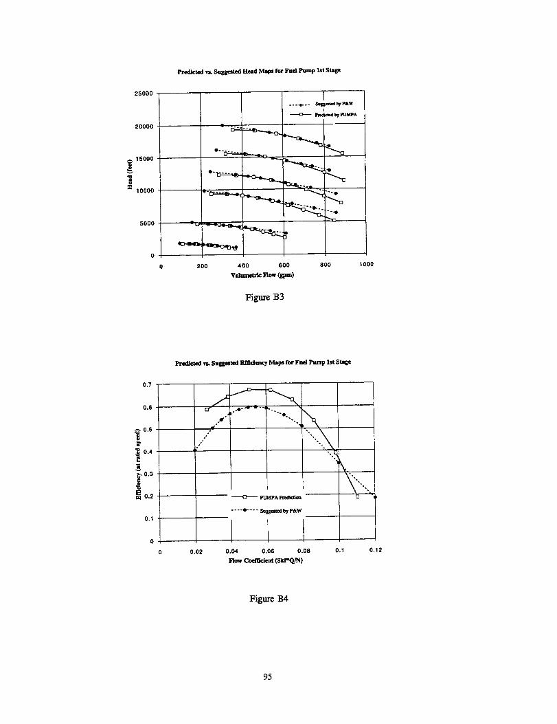
25000

20000

A 15000

lOOOO

5000

Predicted vs. Suggested Head Maps for Fud Pump 1st Stage

D .......

I........ Suggested by P&W

t

Pled_:tcd by PUMPA

"''0

-°.•

200 400 600 800

Volumetric Row (gpm)

Figure B3

1ooo

0.7

0.6

0.5

0.4.=

0.3

_0.2

0.1

Predicted vs. Suggested EII_dencyMaps for Fuel Pump 1st Stage

Jor

.J

oe"If

o°

°o.o

......o---

o ° - ..-°

"4_N

--------(3.---- PUMPAPredt_ou

.... e- - - - Su=cstcd byP&W

0.02 0.04 0.06 0.08

Flow Coemdent (Sk_Q/N)

0.1 0.12

Figure BA

95

25000

Predicted vs. S_ Head Maps for ]Fuel Pump 2rid Stage

20000

_, 15000

10000

5000

o°-°.°,

D---

• o-....... =D--.----.O-

A_

-°°a.

°°- ..° ._,

I--- _-- ° Sulu_cd _y P&W

Rz4i_d by ]'UMPA

,°-•

200 400 600

V,,:umetric Flow (l_m)

Figure B5

800 1000

0.7

0.6

0.5

_. 0.4

¢1

_, 0.3=."0

_0.2

0.1

Predicted vs. Suggested ]gMd_-.y Map for Fuel Pump 2rid Stage

o°9

t •

•_O---- pUMpA i_d_km

.... • .... Sugge_d br px.W

0.02 0.04 0.06 0.08 0.1

FlowCoeM_.m(_P'Q_D

\

0.12 0.14

Figure B6

96

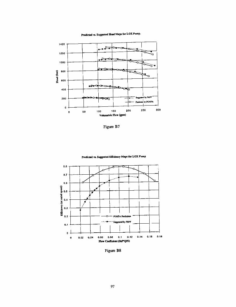
1400

1200

1000

"_ 800

I_ 600

4OO

20O

0

Predicted_ SuggctedHe_iMapsforLOXPump.

L . i,.o_..c_,_

0 50 100 150 200

VolumetricFlow(gpm)

4--;" S-J6-'-;_ bYP&W_

I

250 300

Figure B7

0.8

0.7

0,6

_0.5

0.4iii

o.a"I0E

0.2

0.1

0

0

PrcdicAed vs. Suggested F.Jll_J_y Maps for LOX Pump

S

J

d"oo

/

Y

If

....... t

.Jo_

oO

PUMPA Pngllclion

.... e-- - - Sugg_ted by P&W

0.02 0.04 o.os o,oe o.1 0.12]nowCoemc_t(SkP(_N)

0.14

Figure B8

0.16 0.18

97

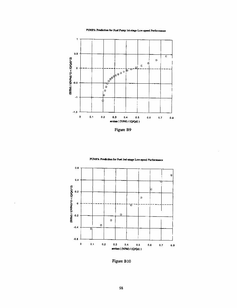
PUMPA Prediction for gud Pump lst-stage Low-speed Performance

0.5

g

÷

_-0.5

-1

-I .5

:l--O-0

0 o

' i0 0

0 oc0

u

O

o

"1

0.1 0.2 0.3 0.4 0.5 o.s

zroma((NINd) I (QIQd))

Figure B9

[3

0m

0.7 0.8

0.6

0.4

0.2

4-

<,,,A 0

|,.= -0.2

-0.4

-0.6

PUMPA Prediction for Fuel 2nd-stage Low-speed Performance

o

o

o

o

0.1 0.2 0.3 0.4 0.5

=ret_ ((N/Nd)/ (Q/Qd))0.6 0.7 0.8

Figure B10

98

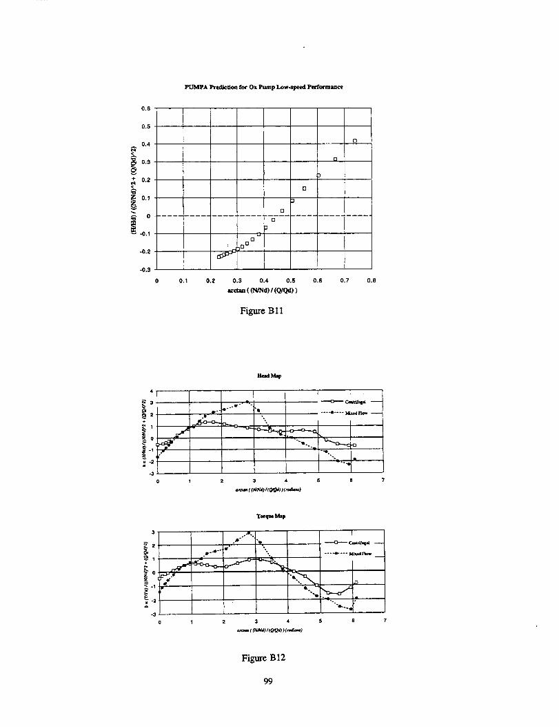
0.6

0.5

0.4

0.3

+ 0.2

_ 0.1

_ 0

_ -0.1

-0.2

-0.3

_A PredlcUon for Ox Pump low-speed Performance

o

o

J

0

0

cIO 0

0

m

[]

3

0.1 0.2 0.3 0.4 0.5

=r¢U= (_/Nd) / (_Od))

0.6 0.7 0.8

Figure Bll

4

÷

_°

= -2.t

-3

!

°,

.@,-'I

Map

D LT @

I L

I

"'11,. _ -G°'o

3 4

,=,=,mt f,W_,) / ((3,_ 1(.,',=,S=u)

5 8

3

°

-1 Is-2

-3

0

o o°• .e

1 2

Torqsm Ms F

JJ., %

D"

f" ",,

½3 4

----e---- MixmlFia_ --

•o ,-° -°

Figure B12

99

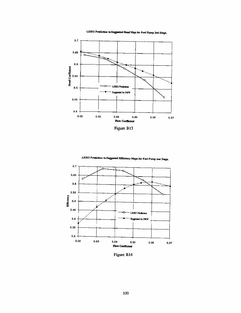
0.7

I._ISO Pred/¢/lo_ vs Suggested B[ead Map for Fuel Pump 2,nd Stage.

0.65

0.6

.=

o.55

I0.5

0.45

0.4

-------13----- LSISO ercd_m

.... e- - -- Suue_d by P&W \

0.02 0.03 0.04 0.05

Flow Coefficient

Figure B13

0.06 0.07

LS]SO PredictiOn v= Sugges_d F,mdency ]Mbsp_ for Fuel Pump 2.ad Stage.

0.7

.=."U

0.65

0.6

0.55

0.5

0.45

0.4

0.35

0.3

oo

.o

°°°

4

o*

oe"°

.°°-

d},,_ t

j.-"

o-

•----0---.- ].3L._O I:'ted_Uoe

.... e- - - - ._:__,¢=_ by P&W

0.02 0.03 0.04 0.05

FlowCormd_

Figure B14

0.06 0.07

I00

Model Prediction - RLIO First Stage FP Head Map

1.4000

1.2000

1.0000

O.BO00

o.eooo

0.4000

0.2000

0.0000

-0.2000

-0.4000

//

/1

/I

J/

Test Data

0.0000 0.2000 0.4000 0.6000 0.8000 1.0000 1.2000 1.4000 1.6000

thee= = m_=a((N/'_d)/(Q_I))

Figure B15

1.4

1.2

A 0.8

0.6÷

0.4

0.2

io-0.2

-0.4

-0.6

R/S Model Prcttlction - RLIO s_ond Stage FP Head Map

I/

/J

J0 0.2 0.4

///

II

¢

Restefir_ld/ScheerPredictions

0.6 0.8 1

a_= - =r=a=((N_aY(O/O_)

1.2

Test )eta

1.4

Figure B16

1.6

I01

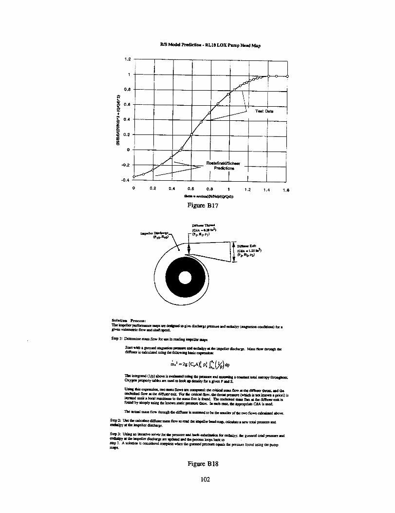
1.2

R/S Model Prcdl_on - RLI8 LOX Pump Head Map

0.8

i 0.6

+

_ 0.4

i_ 0.2

|0

-0.2

-0.4

J

J

J

Roelef_dd/Scheer

Predictions

0 0.2 0.4 0.6 0.8 1

tSm = =_.m((t'_Nd)/(_V_l) )

Figure B17

f _.-.o---

Test Data

1.2 1.4 1.6

(c.._ = _ aJ),HI, Pl)

SoIIUoll I_'oceu:

The i_elkr l_¢rforma_e mal_ are de_ped to give dL_m_ tm_sme md emhalpy (_ cce_ttons) _ agtna vetoer'to now am a_t _e_

Step 1: Detenaiae ma_ flow for me ia teadlng knl_,l_ maps

Sm't v_ a In_ssed s_m pn_'ure _d md_a]l_ m d_ein_eJ_, dlsc_arse. Ma_s flow tl_0ol_ thedt_,m_ = atku]aled u._g lhe tolknmg ba_ exiffiaud_

"I1N _,,_,srmd (l/p) above is ¢va_a_l mdng d_¢lm=mg¢ ¢_1 _11 a _ _ emr_ dm:mglm=.OxY_le= PrqP¢_ ¢=b_sa_ osed=oio_ up ¢iusl_ _ a giv_ p sad S.

Us_ th_ _ _o mass flows me one_med: _he _cal _ss _ = _ _use_ d_. _d tSeu_ed flo_ at _" d_ruse_ e_. Fer the e_l flo_. _e d_ i_u_e (_aich is _ k_a_n a _) _ie='atcdmtii a lvcsdm=dm_ in cb¢massfie= is foond. The ==¢bvk_ rams time at tb¢di,'l'm=- exit is

fouad by _p_y _ Ihe k_y_m stad¢ pte_m_ thes_ Ia ea_ case, the _ CdA is reed.

TI_ _ma_ ma_ flow tlmm_ d_ _ is m_med w be _ I._kr ot-_ _t_ flo_ c_k:ulatcd _.

Step 2: Use _e cak_/=e dMm_ mass flowm readthe_pe.llerbeadmap, cs_ubtea _._ w_l preuu_ _=d=lpy =tb¢ _,,,m._r _=-S¢+

St_p 3: Ushll( a= ilez._lv¢ solve- fro-the prcssm¢ as_dhse_.subslimtkm for mtbalpy, tb¢ guessed total _ =

emba_ a= the impell_ _sd_rse ere upd=_ md the ix,_._.= kx_ps Sack _

s_p|, A so_ut_n L__ comple_ ,who= tb¢ guessed _ equa_ k pmssm.c found osmg the pm_pmaps.

Figure B 18

102

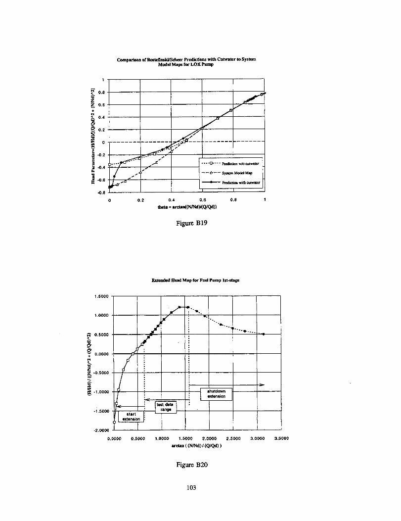
o.5,"o

0.6

÷

0.4

0.2

N,tp

I,-0.2

iI -o.4

3 -o.s¢

-0.8

Compm'bon or Rostelinski/Scheer Predictions wi_ Cutwater to SystemModal Maps for LOX Pump

.... 0---- _ w/o c,.g_ztcr

---- _'---- S_ ModrJ M_p

RmdictiOn_t.b cmwa(_r

I

0 0.2 0.4 0.6 0.8

them = arctaa((N/Nd)/(Q/Qd))

Figure B19

Extended Head Map for Pad Pump lst-stage

1.5000

1.0000

<_ 0.5000

g0.0000

+

_o0.5000

_-1.0000

-i.5000

-2.0000

0.0000

/

I0.5000

"'0

i •"u.

"" .e.

t

shutdown

. | extension

1.0000 1.5000 2.0000

arctan ((N/Nd) / (Q/Qd))

2.5000

)..*"o--°. 6. _

3.0000 3.5000

Figure B20

103

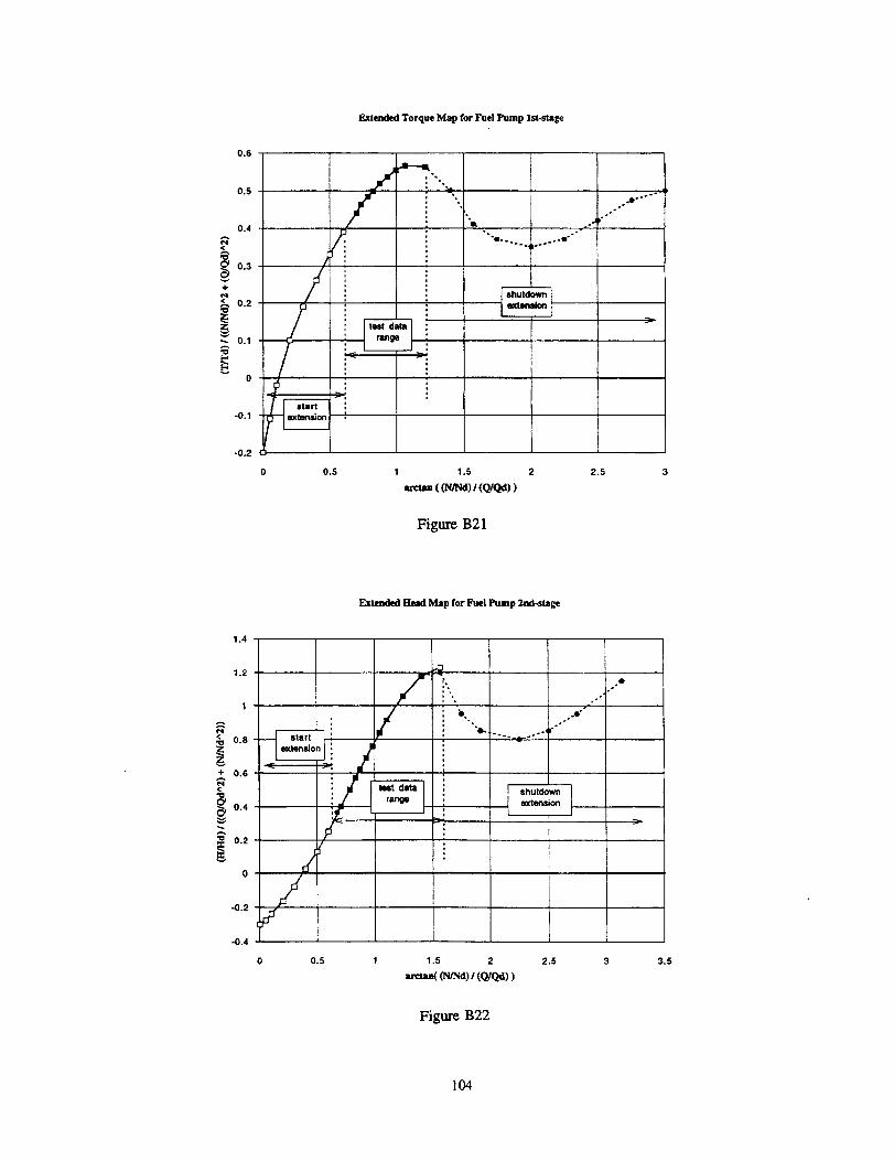
0.6

Extended Torque Map for Fuel Pump Ist-stage

0.4

A

0.3

÷

0.2

--- 0.1A

0

-0.1

0.5

-0.2

,..

; "o

m.-_,

°l .

° .°.o.,

oJ

°°..o. °

..0. oo

ooo.

,o- i

0.5 1 1.5 2

arcUm ((N/Nd) / (Q/Qd))

Figure B21

2.5

Extended Head Map for Fuel Pump 2rid-stage

1.4

1.2

I

•_ 0.8

+ 0.6

<,,,

0.4

_ 0.2

o/-0.2

-0.4

!'°',

0 0.5 1 1.5 2

m'eUm((N/Nd) / (Q/qd))

-°..__.oO"

°

o °O

°-

shutdownextensmn

oo

3.5

Figure B22

104

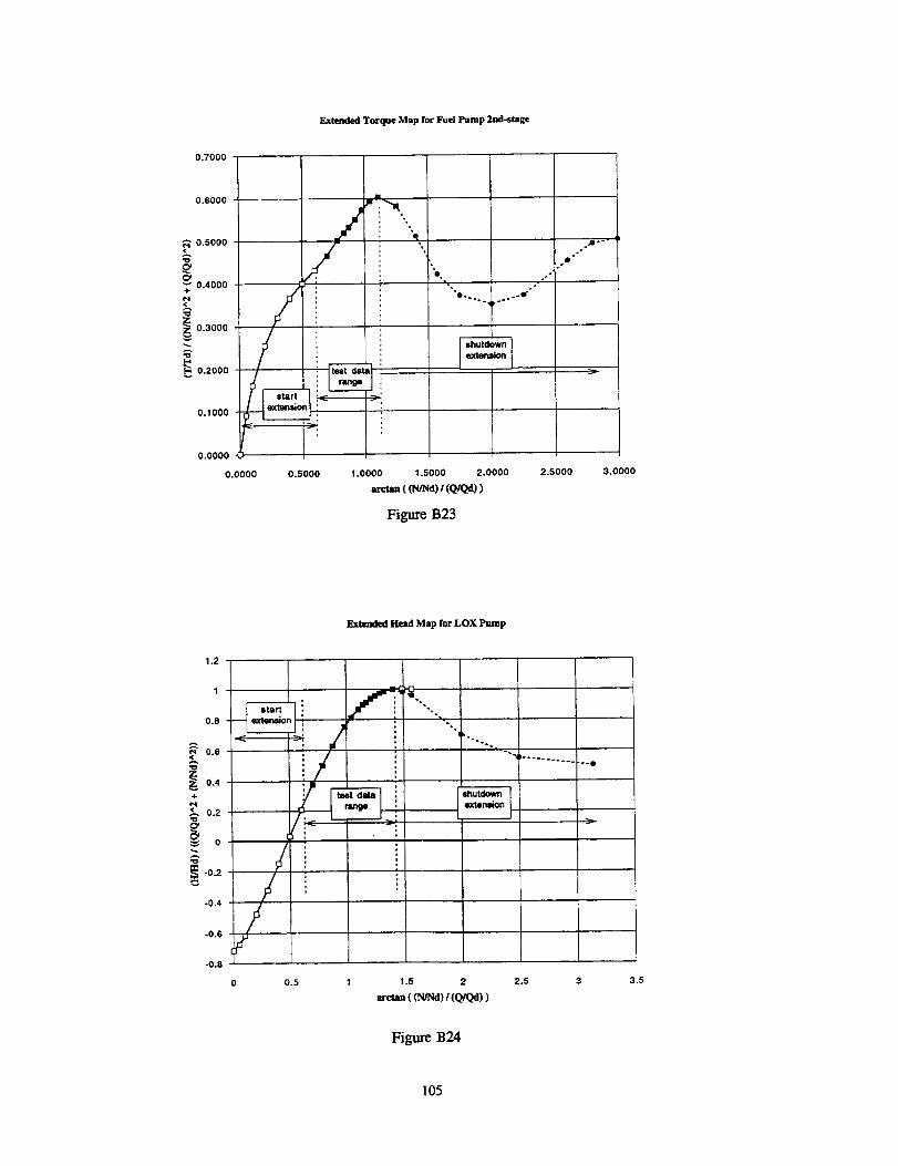
0.7000

0.6000

<_'0.5000

_0.4000÷

_0.3000

_0.2000

0.1000

0.0000

0.0000

start

0.5000

Extended Torque Map for Fud Pump 2nd-stage

/,=_.

i , •

u t

o..... ,-'°

°.°

.o°.a¢

1.0000 1.5000 2.0000

arct.ma ((l"q/Nd) I (Q/Qd))

Figure B23

2.5000

boo-.o°

°m"

3.0000

Extmdml Had Map for LOX Pump

1.2

0.8

0.6

0.4

4.

0.2

0

..-0.2

-0.4

-0.6

-0.8

0 0.5 1 1.5 2

arrt_ ((N/Nd) / (Q/Qd))

2.5

°-o

3.5

Figure B24

105

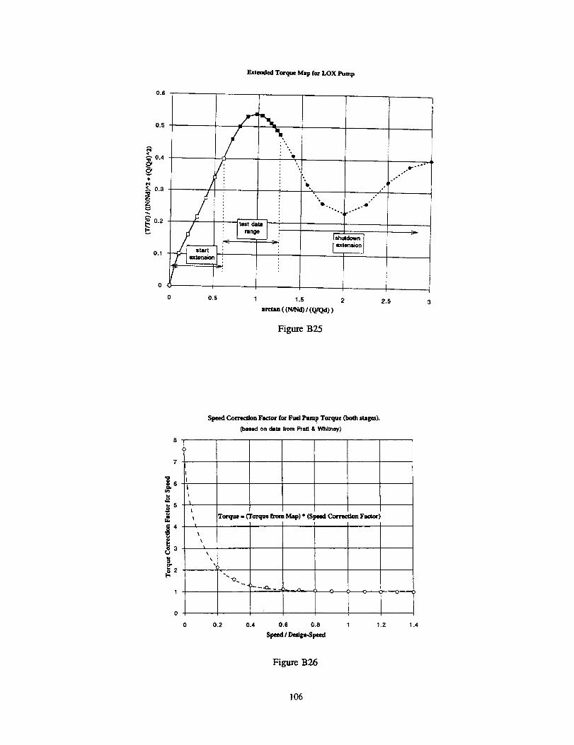
0.6

Extended Torque Map for LOX Pump

0.5

0 0.5

/ -; Q

-, ooo

lb. .4l °

-. , o-o°r

i

0.... -o°

o-oO

°o

:>

1 1.5 2

,,rctaa ((NtNd) / (Q;qd))

2.5

Figure B25

6

,-5

r._3

t

"l\

Speed Correction Factor for Fuel ]Pump Torque (both stages).

on data from Pratt a Whitney)

Torque = (Torque from Map) • (Speed Correction Factor)

0.2

o )

I

0.4 0.8 0.8 1

speed/ V_g_Spced

1.2 1.4

Figure B26

106

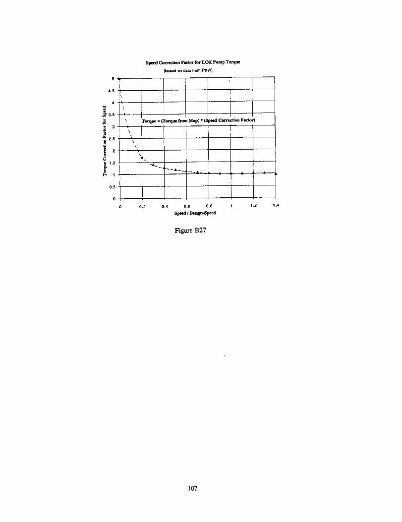
4.5

4

3.£

_o

2.5

1.5

0.5

ll

\

0

0

Speed Correction Factor for LOX Pump Torque

(based on dam from P&W)

ITorque = (Torque from Map) * (Speed Correction Factor)

0.2 0.4 0.6 0.8

Speed?De_g_Speed

1 1.2 1.4

Figure B27

107

APPENDIX C

Component Modeling of RL10 Fuel Turbine

This appendix to the RL10A-3-3A Modeling Project Final Rep.ort describes efforts to predict theperformance of the RL10 fuel turbine using component analysxs programs available to the NASALewis Research Center Space Propulsion Technology Division (SPTD). A cross sectional

representation of the RL10 fuel turbine is shown in Figure C1.

C.1 Analysis Tools UsedThe SPTD has been working to develop turbomachinery design and off-design programs for

several years. Since the RL10 design was already set, only the off-design performance codes wereused in this project The program used to analyze the RL10 fuel turbine is call TURBA (referenceC1). This is a one-dimensional mean-line analysis tool. Given the geometry for the nozzles,rotors and stators, TURBA uses a combination of theoretical and empirical methods to predict the

turbine performance. Basic flow and momentum equations are used to define the interactionbetween the fluid and each row of rotor blades and stators. The geometry of the flow passages is

•calculated to include metal and boundary-layer blockage effects. Design point efficiency is

estimated using an empirical correlation derived from testing of various other turbine designs. Anempirical correlation is also used to characterize the off-design-point efflciencies. It is possible to

adjust the assumed fluid losses through the turbine to better match test data if desired.

C.2 Predictions from TURBA codeTURBA was used to analyze the performance of the RL10 fuel turbine, which has two stages.

Figures C2 through C5 show the predicted flow parameters (related to.the fluid res_tan, ce)aedefficiencies of the turbine stages. The turbine performance maps provlaea t_y t-ratt _ w m y(and presumed to be based on test data) are for both stages combined, rather than for each stageindividually. These maps are shown in Figures C6 and C7. The flow resistance is represented byan effective orifice Cd*Area as a function of overall speed-ratio and pressure-ratio. The combined-

two-stage efficiency of the turbine is also given as a function of overall speed-ratio. The way inwhich the turbine stage performance maps have been combined by Pratt &Whitney makes it

difficult to perform one-to-one comparisons with the TURBA predictions.

In order to compare the combined maps provided by .Pratt & Wlai'mey with .the s!ng!e-stage .maps

predicted by TURBA, each set was used in a simulaUon wmcn oermes sma,_ar s,n.att spe,e 9, ml.e_tand exit conditions. From these simulations, me mass xtowrates ana overatt turome e_rlcxencxesfrom the two models can be compared. These results are shown in Figures C8 and C9 asfunctions of shaft speed at several pressure-ratios. These figures indicate that the TURBA

predictions for efficiency and flow resistance differ significantly (at least 5%) from the P&Wvalues, especially at very low speeds.

Due to schedule limitations, it was not possible to investigate the differences between the TURBA

predictions and P&W-specified maps in detail. Although the maps from Pratt & Whitney appear tobe based on test-data, there are some issues regarding these maps which warrant further

investigation in the future (resources permitting.). In particular, it has been noted that the turbineperformance maps suggested for the start-transient model are different from those suggested for thesteady-state system model The TUR_A simulations were not as exhaustive as those for pump

performance and should also be evaluated in the future, resources permitting.

C.3 Sensitivity of System Model to Turbine Performance VariationsAs discussed in section 4.1.2.4 of the report, it has been found that the timing of the RL10 engine

start is extremely sensitive to small variations in the turbine efficiency and flow resistance.Consider the two efficiency maps shown in Figure C10. The curves shown here are two

polynomials intended to fit the same test data, but with different assumptions for order and residualerror. Although they are quite similar overall, the slopes of the two curves differ by approximately

109

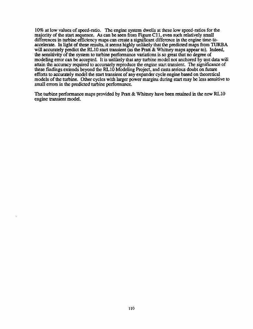
10%at low valuesof speed-ratio. The engine system dwells at these low speed-ratios for themajority of the start sequence. As can be seen from Figure Cll, even such relatively smalldifferences in turbine efficiency maps can create a significant difference in the engine tirne-to-accelerate. In light of these results, it seems highly unlikely that the predicted maps from TURBAwill accurately predict the RL10 start transient (as the Pratt & Whitney maps appear to). Indeed,the sensitivity of the system to turbine performance variations is so great that no degree ofmodeling error can be accepted. It is unlikely that any turbine model not anchored by test data willattain the accuracy required to accurately reproduce the engine start transient. The significance ofthese findings extends beyond the RL10 Modeling Project, and casts serious doubt on futureefforts to accurately model the start transient of any expander cycle engine based on theoreticalmodels of the turbine. Other cycles with larger power margins during start may be less sensitive tosmall errors in the predicted turbine performance.

The turbine performance maps provided by Pratt & Whitney have been retained in the new RL10engine transient model.

110

Glossary

Speed Ratio" Turbine blade tip velocity divided by nozzle spouting velocity.

N*D*r_U--

60

c o = 5/2g*J*AH,o..le

Speed Ratio = u/c0

Reduced Speed : Rotation Rate (in rpm) divided by the square root of the inlet temperature (R).

N

Reduced Speed =

Flow Parameter" multiplying the flow parameter by the inlet pressure divided by the square-root

of the inlet temperature gives the mass flow rate.

Flow Parameter = Pi,_t

C1.

References

Veres, J., Axial Turbine Design and Off-Design Performance Prediction (TURBA),NASA TM (number pending), 1995.

111

Turbine .?,nd-Stage Turbine lst-StageRotor Rotor

Exit Guide VanesSllltor

II

Inlet N_zle

Figure C1

1.40

RL10A.-3-3A TURBINE

STAGE ONE PERFORMANCE

1.35

1.3od

1.25re

1.1.1n-

1.20or}o'}ILlI¢ 1.15a.

//

/

./

.1

1.10 /".,,1' /

.,,.." jJ

1.05 t

1.00 , , , , I f _ _ , I ,

0.00 0.05 0.10

i I

i /

itl

I /

t io

I //

/

/

I

..... lsoswff-- 1641

......... 1063 N/Y_"

.... _i _

, I a , , , I

0.15 0.20

FLOW PARAMETER

Figure C2

]12

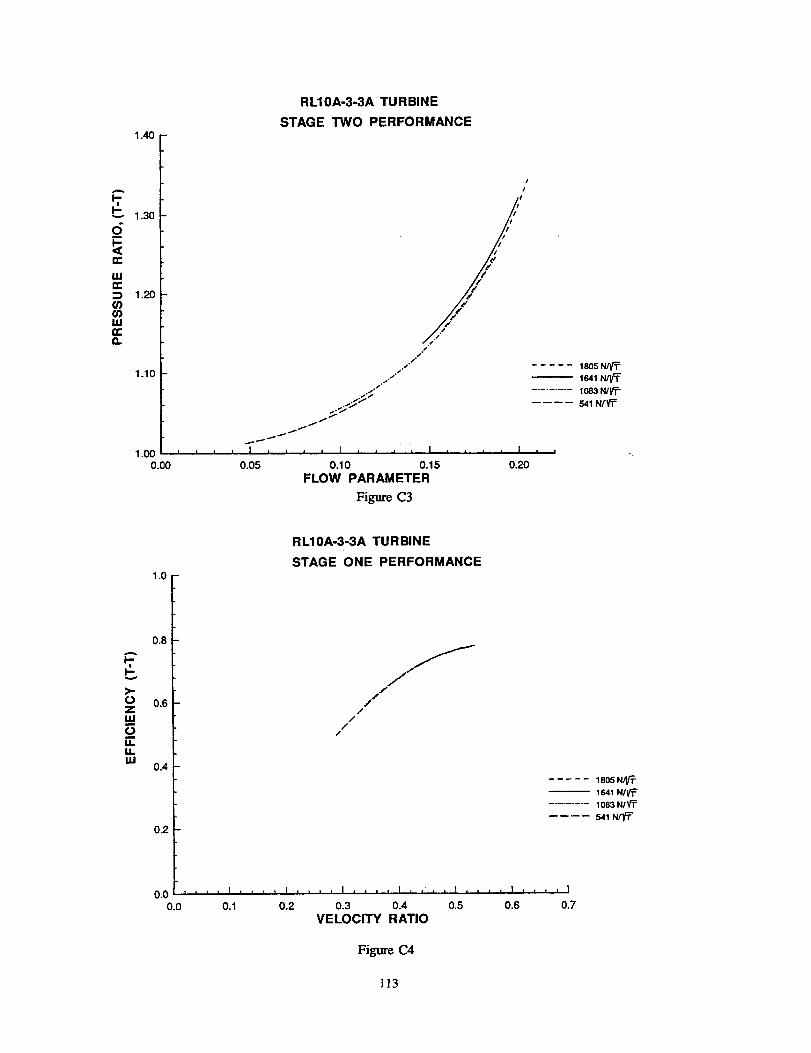
1.40

RL10A-3-3A TURBINE

STAGE TWO PERFORMANCE

1.30

n-

u.I

1.20o)o_I¢1n-o.

1.10

1.000.00

Figure C3

1,0 --

RL10A-3-3A TURBINE

STAGE ONE PERFORMANCE

0.8

I--

>-O 0.6Zu.I

14.W

0.4

0.2

0.00.0

/

//

//

..... 1sosNN_1641wVF

......... 1083 NIV'T

.... 541N/_

t i i i { i i I, I .... I .... I, ,',, I,, , , I .... 1

0.1 0.2 0.3 0.4 0.5 0.6 0.7VELOCITY RATIO

Figure C4

113

1.0

RL10A-3-3A TURBINE

STAGE TWO PERFORMANCE

AI-

>-OZLU

0

u.U.Ul

0.8

0.6

0.4

O_

0.0

0.0

//

/#

, , , , I .... I , , , _ I , , , , I , , , , I , , , , I .... I

0.1 0.2 0.3 0.4 0.5 0.6 0.7

VELOCITY RATIO

..... 1805 N/irf

--- 1_1 N/rf......... 10_ Nl_f

.... ,_1_

Figure C5

0.8

0.7

0.6

0.5

¢=

"I_ 0.4

E

0.3

0.2

0.1

///

0 0.1 0.2

1_IOA.3-3A Fuel Turbine l_iden¢ 7

--o-- _o...

0.3 0.4 ().5

Velocity RaUo (U/Co):

0.6 0.7

Figure C6

0.8

114

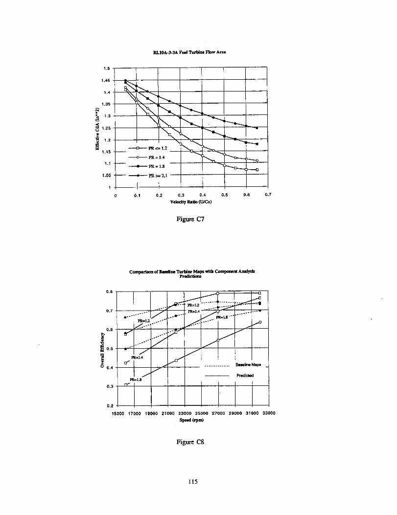
RL10A-3-3A Fuel Turbine Flow Area

1.5

1.45

1.4

1.35

_ 1.3

1.25_J

. 1.2

1.15

1.1

1.05

PR <=

-----o-_ PR = 1.4

_ PR= 1.8

-- --------a-----PR >= 2.1

! t0 0,1 0.2 0.3 0.4

Vdodt7 Ratte (U/Co)

Figure C7

_ ........_

0.5 0.6 0.7

Comparison of Bmdine Turbine Maps with Component AnalysisPredictions

0.8

0.7

0.6

0.5

0 0.4

..°-°-"

0°- o

PR_1.2

.°-

°_°°o°°

J" J1_=1.4

JP!_1.8

O.3 r'_

0.2

.. °-"

o° °°*°_

_ .g

f

J

.-" _13

JJ

_°..°-*°

ff

o

Predicted

15000 17000 19000 21000 23000 25000 27000 29000 31000 33000

Speed (rpm)

Figure C8

115

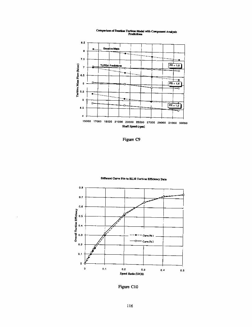
8,5

7.5

7

o_ 6.5

6

"= 5.5

5

Compm'Json of Baseline Turbine Model with Component AnalysisPredictions

4.5

O-..

! I

..... 41"• -. °°,

TURBA Predlc_orB

---...."°--°.., L-..O. °

'-°.....

°-- ..,4,

-. ......

"°--° ..... ..

,-.Q

: ....... "'-'O

o

D._. _ ___o... - .........

15000 17000 19000 21000 23000 25000 27000 29000 31000 33000

ShaftSpeed(rpm)

Figure C9

0.8

Difrecent Curve Fits to RLIO Turbine EfTJden_ Data

0.7

0.6

o="0 0.5

0.4

0.3

0

0.2

0.1

i//

/./

0 0.1

/

----o---- C=_eRt ! ,

Cmw¢ Fit 2

0.2 0.3

Speed Ratio (U/C0)

0.4 0.5

Figure C10

116

(D

_D

CD

[_13_

C-(D

ra

E_D

r-

50O

400

30C

2OO

IO0

10

RL IOA-3-3A Start

_uRVE F,T _ . ___9____F__T'_____

ii iiii

0 10.5 1

/

I

IIII

I

I!

Ii

iIi

I

.0

/fi

I

/

/

i t

iI

#

: /

JIi i i i i

!I .5 12.0Time

/

i i i •

12.5 13.0 '13.5

Figure Cll

117

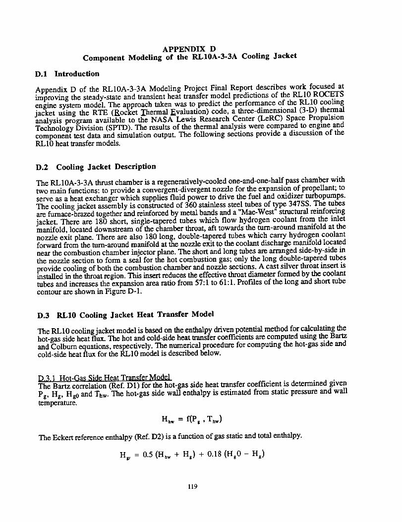
APPENDIX D

Component Modeling of the RL10A-3-3A Cooling Jacket

D.1 Introduction

Appendix D of the RL10A-3-3A Modeling Project Final Report describes work focused atimproving the steady-state and transient heat transfer model predictions of the RL10 ROCETSengine system model. The approach taken was to predict the performance of the RL10 coolingjacket using the RTE (Rocket Thermal Evaluation) code, a three-dimensional (3-D) thermalanalysis program available to the NASA Lewis Research Center (LeRC) Space PropulsionTechnology Division (SPTD). The results of the thermal analysis were compared to engine andcomponent test data and simulation output. The following sections provide a discussion of theRL10 heat transfer models.

D.2 Cooling Jacket Description

The RL10A-3-3A thrust chamber is a regeneratively-cooled one-and-one-half pass chamber withtwo main functions: to provide a convergent-divergent nozzle for the expansion of propellant; toserve as a heat exchanger which supplies fluid power to drive the fuel and oxidizer turbopumps.The cooling jacket assembly is constructed of 360 stainless steel tubes of type 347SS. The tubesare furnace-brazed together and reinforced by metal bands and a "Mac-West" structural reinforcingjacket. There are 180 short, single-tapered tubes which flow hydrogen coolant from the inletmanifold, located downstream of the chamber throat, aft towards the turn-around manifold at thenozzle exit plane. There are also 180 long, double-tapered tubes which carry hydrogen coolantforward from the turn-around manifold at the nozzle exit to the coolant discharge manifold locatednear the combustion chamber injector plane. The short and long tubes are arranged side-by-side inthe nozzle section to form a seal for the hot combustion gas; only the long double-tapered tubes

provide cooling of both the combustion chamber and nozzle sections. A cast silver throat insert isinstalled in the throat region. This insert reduces the effective throat diameter formed by the coolanttubes and increases the expansion area ratio from 57:1 to 61:1. Prof'fles of the long and short tubecontour are shown in Figure D-1.

D.3 RL10 Cooling Jacket Heat Transfer Model

The RL10 cooling jacket model is based on the enthalpy driven potential method for calculating thehot-gas side heat flux. The hot and cold-side heat transfer coefficients are computed using the Bartzand Colburn equations, respectively. The numerical procedure for computing the hot-gas side andcold-side heat flux for the RL10 model is described below.

D.3.1 Hot-Gas Side Heat Transfer ModelThe Bartz correlation (Ref. D1) for the hot-gas side heat transfer coefficient is determined given

Pg, Hg, Hg0 and Thw. The hot-gas side wall enthalpy is estimated from static pressure and wall

temperature.

Hhw -- f(Pg , T_,,)

The Eckert reference enthalpy (Ref. D2) is a function of gas static and total enthalpy.

Hs_ = 0.5 (H,w + H e) + 0.18 (Hg0 - Hg)

119

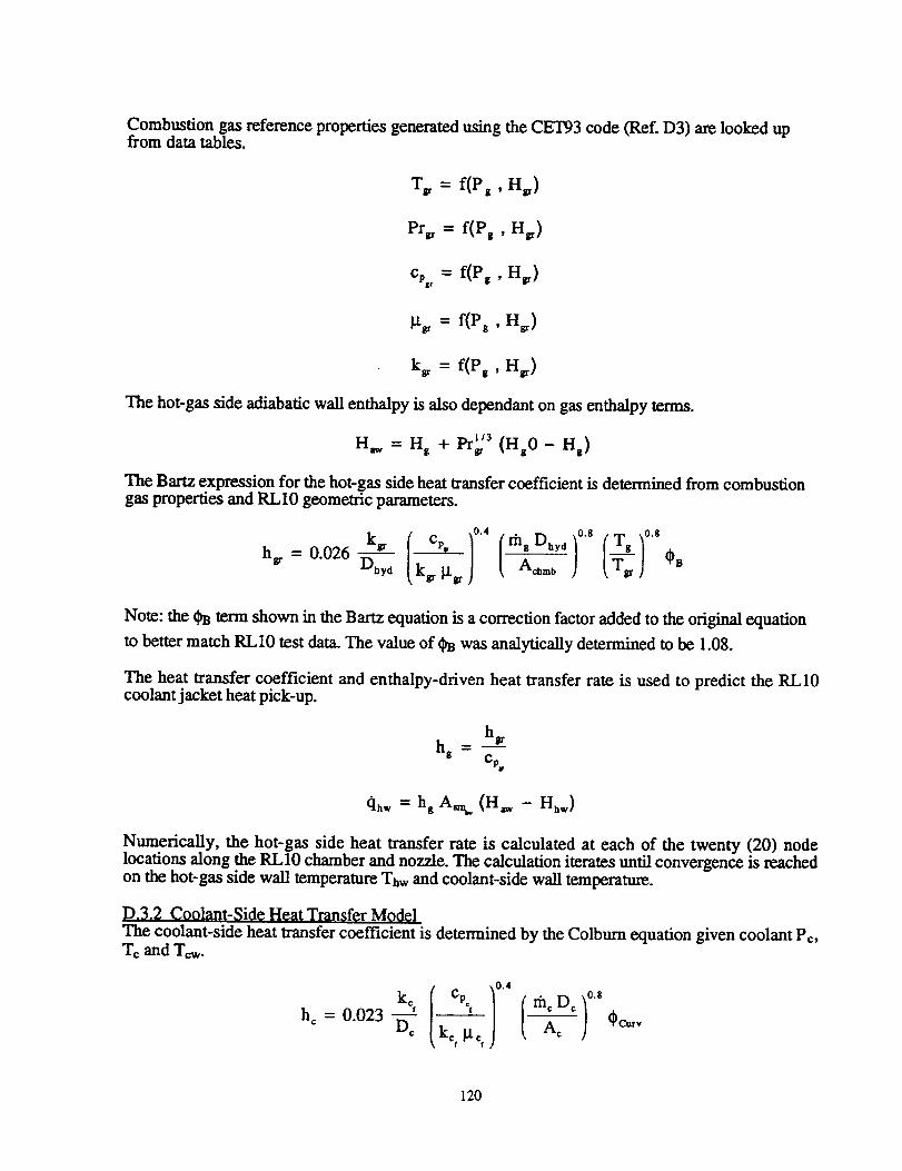
Combustion gas reference properties generated using the CET93 code (Ref. D3) are looked upfrom data tables.

Ts' = f(P8 ' H_)

Prv = f(Pg , Hsr)

Cp,, = f(P_ ,H_)

lit_ = f(P_ , Hgr)

k_ = f(Ps ' Hsr)

The hot-gas side adiabatic wall enthalpy is also dependant on gas enthalpy terms.

113

H_ = Hg + _r_ (Hg0- He)

The Bartz expression for the hot-gas side heat transfer coefficient is determined from combustiongas properties and RL10 geometric parameters.

=0.026 k, / c,. ]0.,. )0.s )0.,h_. _ (k_, { m-_ D'_ ° {T_ Ce

Note: the ¢B term shown in the Bartz equation is a correction factor added to the original equation

to better match RL10 test data. The value of 0B was analytically determined to be 1.08.

The heat transfer coefficient and enthalpy-driven heat transfer rate is used to predict the RL10coolant jacket heat pick-up.

hgr

h s -c_

qh,,= hs Am,. (Haw - Hhw )

Numerically, the hot-gas side heat transfer rate is calculated at each of the twenty (20) nodelocations along the RL10 chamber and nozzle. The calculation iterates until convergence is reachedon the hot-gas side wall temperature Thw and coolant-side wall temperature.

D.3.2 Coolant-Side Heat Transfer Model

The coolant-side heat transfer coefficient is determined by the Colbum equation given coolant Pc,Tc and T_.

kcf / Cp©f )0.4h. =0.023 _ (kc _t¢

120

Coolantpropertiesareevaluatedatthestaticpressureandf'flmtemperature.

T, + T,.,,T_ - 2

A correction factor for the tube radius of curvature (Ref. D4) accounts for heat transfer

enhancement in the throat and nozzle inlet regions.

In the above expression, D c is the hydraulic diameter of the coolant passage, Rc_-,, is the radius of

curvature, the positive (+) sign denotes concave curvature and the negative sign (-) indicates

convex curvature.

The heat transfer rate to the coolant through the cold-side boundary layer is determined by a forced-

convection temperature difference equation.

dl,_, = h_ Am (T,.,, - T,)

I9.3.3 Conduction Heat Transfer ModelThe heat transfer rate across the tube metal wall is calculated by the conduction equation.

elm = km A._ 8, (Th,,, -- T,.,,)

Thermal conductivity is determined at the average metal wall temperature.

T_,, + Th,,

T=- 2

D.4 RTE Analytical Model

This section describes the RTE analytical program (Ref. D5) used in the evaluation of the RL10

cooling jacket model. Heat flux, wall temperature and coolant temperature and pressure profiles

were predicted for the RL10 using this code. Minor modifications were required to RTE for

analyzing the RL10's tubular coolant passage geometry.

The RTE code, developed under grant for the NASA LeRC SPTD, is a 3-D model for analyzing

the thermal performance of regeneratively-cooled thrust chambers. The main inputs to the RTEcode are coolant inlet temperature and pressure, coolant passage dimensions, nozzle coordinatesand chamber conditions; chamber pressure, mixture ratio (O/F) and chamber mass flowrate. The

analysis accounts for coolant passage radius of curvature effects, surface roughness and coolantentrance effects. Heat transfer on both the hot-gas side and coolant-side of the tube wall are

predicted, as well as the momentum and frictional losses of the coolant flowing through the tubes.Frictional losses are computed using the Darcy correlation (Ref. D6), modified to account for the

coolant density change between stations. RTE uses either a temperature-driven or optionalenthalpy-driven potential method for estimating heat flux. The Colburn correlation is used to

predict heat transfer coefficients on the hot-gas side. The coolant side heat transfer is alsocomputed using the Colbum correlation with corrections to account for the tube curvature effect.

121

This effect causes the coolant-side heat transfer rate to alternately increase and decrease due toboundary layer thinning as the fluid's momentum forces coolant against the hot-side (concave) andcold-side (convex) of the tube wall (Ref. D7). Heat transfer enhancement (Figure D-2) occurs asthe coolant progresses through the throat and then through the chamber convergent section regions,res.pectively. RTE uses a one-dimensional equilibrium code (CE_9) to obtain hot-gas side thermalana transport properties. Hydrogen coolant properties are obtained by RTE from the GASP code(Ref. D8).

D.5 RL10 Predictions using RTE

D.5.1 Baseline RTE analytical results

To determine the effects of spatial resolution, the RL10 cooling jacket was modeled with the RTEcode at varying numbers of computational nodes. Figure D-3 shows the RTE predictionsconverging at a spatial resolution of approximately twenty axial nodes. This indicated thatincreasing the number of nodes above twenty had little or no effect on predicted heat flux. Basedon this "optimized" result, a twenty-node RL10 coolant jacket model was constructed for the RL10system model.

A comparison was then made of a twenty-node RTE model of the RL10 with limited test data andP&W results that were available. RTE predictions of heat flux, hot-gas side wall temperature,coolant pressure and coolant temperature are compared to "typical" P&W analytical results inFigures D-4 through D-7. Comparing the RTE predictions with Pratt & Whitney's own analysisshowed that they are basically similar. Figure D-4 shows that the original RL10 heat transfer modelis in poor agreement with both the RTE and P&W analyses. Figures D-6 and D-7 compare theRTE model predictions with the RL10 test data for coolant pressure drop (AP) and temperature rise(AT). Heat flux, wall temperature, cooling jacket pressures and temperatures are not measured atintermediate points along the cooling jacket so detailed data was not available to validate the RTEpredictions.

RTE is limited to the analysis of single-pass, counter-flow cooled thrust chambers. In order toanalyze the RL10 with this code, the half-pass, 180 short tubes of the RL10 chamber was treated

as strictly counter-flow in the RTE model. The predicted RTE coolant temperature profile shown inFigure D-7 illustrates this effect. The RTE analysis was constructed such that liquid hydrogencoolant entered the jacket at the nozzle exit plane. The coolant inlet temperature used in the analysiswas 58oR.

D.6 RL10 Cooling Jacket System Model Construction

D.6.1 Twenty-node RL10 system model subrou_.Based on the RTE analysis for variable nodes, the initial cooling jacket heat transfer subroutinecreated for the RL10 system model included all twenty (20) thermal and coolant fluid axial-nodesused in RTE. A new combustion gas property routine for the RL10 model was generated fromCET93 (Ref. D3). Tables of thermal and transport property data for each hot-gas side axial nodewere produced. Hydrogen coolant properties for the RL10 system model are obtained from anextensive set of built-in data tables. A comparison of GASP output used by RTE with the existingRL10 hydrogen property data tables indicated no significant differences.

D.6.2 Rea_uired corrections to better match RL10 engine te_t dat_During the initial phase of the RL10 analysis, large discrepancies were noted between predictedand measured values of overall cooling jacket pressure drop and temperature rise. It appeared that

122

the RYE model seriously under-estimated experimental coolant AT and _tP. It was later ascertained

that the predictions did match fairly well within P&W's predictions and other engine test cases.There apparently is a large variation in heat transfer and frictional loss between different enginesoperating at nearly identical conditions. These engine-to-engine variations appear to be about 10percent in total heat pick-up and coolant AP, but there is insufficient test data to confum this with

any confidence.

Another assumption which effects the RL10 coolant jacket heat transfer model is the percen.tage nO_tube surface area which is exposed to hot-gas side heat transter, tmw neat transter preaicuocould result by assuming too low of an exposed tube surface area. A value of 112 degrees wasspecified by Pratt & Whitney. It is possible that their value is specifically tuned to P&W's owncalculation technique. It is also possible that the actual effective tube surface area is different fromengine-to-engine due to manufacturing variations. As long as the heat pick-up is sufficient to startthe engine, the engine will not be rejected in manufacturing.

Several experts concede that the state-of-the-art in heat transfer prediction is on the order of 10% to20% accuracy (Ref. D9). The discrepancies noted above, while undesirable for system analysis,are within the generally accepted range of accuracy for thrust chamber heat transfer models.Ultimately, given the uncertainties in test-to-test variations, a factor of 0.028 in the Bartz equationwas employed in the RL10 system model instead of the more generally accepted value of 0.026. Itwas also determined that a friction factor approximately 94 percent of that recommended by P&W

would improve the coolant AP predictions.

1).6.3 Enthaltw vs Temoerature potential drivin_ heat transferThe analyses-fimher indicated th-at when the Ba_'tz or Colbum heat transfer coefficient was used ina temperature-driven heat-transfer equation, the model did not correctly predict the variation inRL10 heat transfer with chamber mixture ratio.

dlh.= hg A,_. (T_ - Th.)

The enthalpy-driven correlation provided a much more accurate model of the heat transfer ratevariation with mixture ratio as shown by the RYE results in Figure D-8. The total heat pick-up

increased by 6.4% over the test data O/F range of 4.7 to 5.7.

dlh,, = h a A_. (Haw - Hhw )

D.6.4 Twenty vs Hve Coolant orooertv nodesThe final issue to be addressed-w_ the integration of the full twenty-node cooling jacket model

with the rest of the RL10 engine transient model. Includ.ing.sep.arate dyn. amic fluid volumes for

each node was possible but the size of the Jacobian matrix slgmtlcanuy mcreasea, it naa .atreaaybeen shown that a five-node model gave serious discrepancies in the wall heat transfer distribuUon.It was found, however, that if twenty hot-gas nodes and twenty metal nodes were properlyconnected to five coolant nodes, the heat transfer distribution could be satisfactorily modeled while

keeping the Jacobian matrix size to a minimum. A comparison of the full twenty-node model andthe proposed hybrid model yielded comparable results for cooling jacket wall temperature, heatflux and coolant temperature. Only the coolant static pressure result of the hybrid model showedsome underestimation when compared to the twenty-node model.

The final RL10 cooling jacket model installed in the engine system model consisted of volume

123

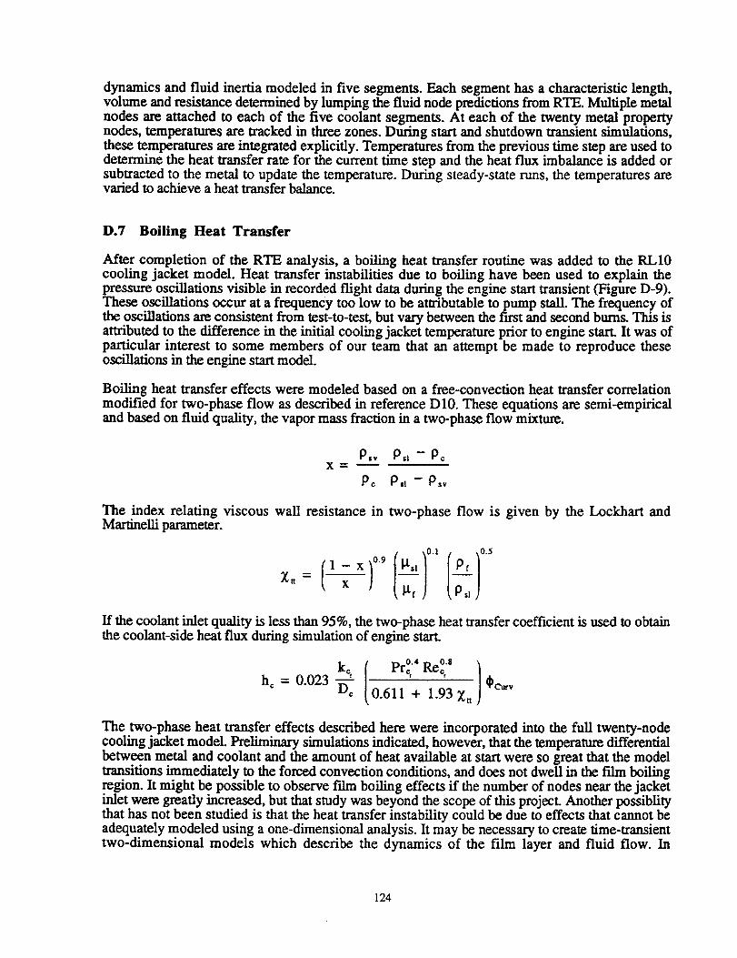
dynamics and fluid inertia modeled in five segments. Each segment has a characteristic length,volume and resistance determined by lumping the fluid node predictions from RTE. Multiple metalnodes are attached to each of the five coolant segments. At each of the twenty metal propertynodes, temperatures are tracked in three zones. During start and shutdown transient simulations,these temperatures are integrated explicitly. Temperatures from the previous time step are used todetermine the heat transfer rate for the current time step and the heat flux imbalance is added orsubtracted to the metal to update the temperature. During steady-state runs, the temperatures arevaried to achieve a heat transfer balance.

D.7 Boiling Heat Transfer

After completion of the RTE analysis, a boiling heat transfer routine was added to the RL10cooling jacket model. Heat transfer instabilities due to boiling have been used to explain thepressure oscillations visible in recorded flight data during the engine start transient (Figure D-9).These oscillations occur at a frequency too low to be attributable to pump stall. The frequency ofthe oscillations are consistent from test-to-test, but vary between the first and second burns. This isattributed to the difference in the initial cooling jacket temperature prior to engine start. It was ofparticular interest to some members of our team that an attempt be made to reproduce theseoscillations in the engine start model.

Boiling heat transfer effects were modeled based on a free-convection heat transfer correlationmodified for two-phase flow as described in reference D10. These equations are semi-empiricaland based on fluid quality, the vapor mass fraction in a two-phase flow mixture.

X

P,, P,_ - pc

Po P,1 - P,,

The index relating viscous wall resistance in two-phase flow is given by the Lockhart andMartinelli parameter.

_tt _

If the coolant inlet quality is less than 95%, the two-phase heat transfer coefficient is used to obtainthe coolant-side heat flux during simulation of engine start.

pro .` Re°" /

)0.611 + 1.93 Za

The two-phase heat transfer effects described here were incorporated into the full twenty-nodecooling jacket model. Preliminary simulations indicated, however, that the temperature differentialbetween metal and coolant and the amount of heat available at start were so great that the modeltransitions immediately to the forced convection conditions, and does not dwell in the film boilingregion. It might be possible to observe film boiling effects if the number of nodes near the jacketinlet were greatly increased, but that study was beyond the scope of this project. Another possiblitythat has not been studied is that the heat transfer instability could be due to effects that cannot beadequately modeled using a one-dimensional analysis. It may be necessary to create time-transienttwo-dimensional models which describe the dynamics of the film layer and fluid flow. In

124

summary, the 1-D film boiling model was included in the RL10 engine system model. This modelis also based on only five coolant-fluid property nodes. No effects of film boiling have beenobserved in any of the RL10 simulations performed thus far.

125

Nomenclature

Achmb --

Asm =

D c =

D h =

Cp

h =

H =

k =

m =

P =

Pc --"

Pr =

q =

Rcurv =

Re =

T =

V =

X

Greek

Xtt

_x =

_t =

p =

cross-sectional flow area of coolant tube (in2)

cross-sectional area of hot-gas-side chamber (in2)

metal surface area (in2)

hydraulic diameter of coolant tube (in)

hydraulic diameter for chamber hot-gas flow (in)

heat capacity at constant pressure (Btuflbm-oR)

heat transfer coefficient (Btu/sec-in2-oR)

enthalpy (Btu/lbm)

thermal conductivity (Btu/sec-in-oR)

mass flow rate (Ibm/see)

smile pressure (lbf/in2)

chamber pressure (Ibf/in2)

Prandfl number 0.t cp / k)

heat transfer rate (Btu/sec)

coolant tube radius of curvature (in)

coolant Reynolds number (me Dc / _ A¢)

temperature (oR)

volume (in3)

quality, vapor mass fraction

Symbols

= Lockhart and MartineUi parameter

wall metal thickness (in)

absolute viscosity (Ibm/'m-sec)

density flbm/ft3)

126

q_Curv =

Subscripts

aw --

c

cw --

f =

g =

hw =

m

r

S] =

sm =

sv

0 =

empirical correction to the Bartz equation for the RL10 (1.08)

correction factor for radius of curvature effect

adiabatic wall

bulk coolant

cold-side wall metal

film

free-stream combustion gas condition

hot-side wall metal

metal

hot-gas reference condition

saturated liquid

surface of metal

saturated vapor

total or stagnation

127

References

D1 Bartz, D. R., "Survey of Relationships between Theory and Experiment for ConvectionHeat Transfer in Rocket Combustion Gases", Advances in Rocket Propulsion, AGARD,Technivision Services, Manchester, England, 1968.

D2 Eckert, E. R. G., and Drake, R. M., "Analysis of Heat and Mass Transfer", McGraw-Hill,1972.

D3 McBride, B. J., Reno, M. A., and Grodon, S., "CET93 and CETPC: An Interim UpdatedVersion of the NASA Lewis Computer Program for Calculating Complex ChemicalEquilibria With Applications", NASA TM-4557, March, 1994.

D4 Owhadi, A., Bell, K. J., and Crain, B., "Forced Convection Boiling Inside H e 1 i c a 11 y-Coiled Tubes", Int'l Journal of Heat and Mass Transfer, Vol. 11, pp. 1779-1793, 1968.

D5 Naraghi, M. H. N., "RTE - A Computer Code for Three-Dimensional Rocket ThermalEvaluation", Prepared for the NASA Lewis Research Center, Grant NAG 3-8892, July1991.

D6 Moody, L. F., "Friction Factors for Pipe Flow", Transactions of ASME, pp. 671-684,1944.

137 Hendricks, R. C., Simoneau, R. J., and Smith, R. V., "Survey of Heat Transfer to NearCritical Fluids", Advances in Cryogenic Engineering, Vol. 15, pp 197-237, Plenum Press,1970.

D8 Hendricks, R. C., Baron, A., Peller, I., and Pew, K. J., "GASP - A Computer Code forCalculating the Thermodynamic and Transport Properties for Eight Fluids - Helium,Methane, Neon, Nitrogen, Carbon Monoxide, Oxygen, Argon, and Carbon Dioxide",Presented at the XIII Int'l Congress of Refrigeration, NAS/NRC, Washington D.C.,1971.

D9 Quentmeyer, R. J., NYMA Inc., Cleveland, OH, personal communication, August 1994.

D10 Hendricks, R. C., Graham, R. W., and Friedman, R., "Experimental Heat Transfer andPressure Drop of Liquid Hydrogen Flowing Through a Heated Tube", NASA TN D-765,1961.

128

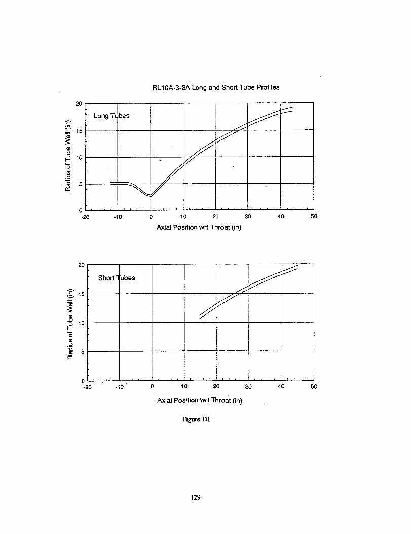
20

"E""" 15

Q)JE_

10!-

0

.__"10

m 5rr

0-20

RLIOA-3-3A Long and Short Tube Profiles

Long Tt

/J

i t i

0 20 30

//

T I

40 50

Axial Position wrt Throat (in)

2o

A

c 15

-_ 10}-

0

__

n-

0-20

Short "1ubes

ifff

-10

!

i

1 t ! I I 1 I ' , , t I

10 20 30

Axial Position wrt Throat (in)

Figure D1

, i40 50

129

2.5

2.0

hEXPT

hCALC

1.5

1.00

Tube Curvature Effect on the LH2 Heat TransferCoefficient for a Concave Surface (Ref. D3)

/ \\

\

\

%

• ILog (R ©/R hyd )

Figure D2

25

2O

c-

c)15

u.10

0"!- 6

RTE Model of RL10 - Effect of Computational Nodes on Heal Flux

i

i.!!//_ _ _

.!/__ _ !

----m---- RTE 60 Fluid I k)des

-10 10 2o 50

Axial Distance wwrt Throat (in)

--O-- RTE 20 _ I lodes

-- "_"-- RTE 8 Rui¢l I_ =dU

-.--O-.-- R'rE5 _ _ _

I

\

_'_ *-..'t_')_ ,' , , . i i i i

Figure D3

130

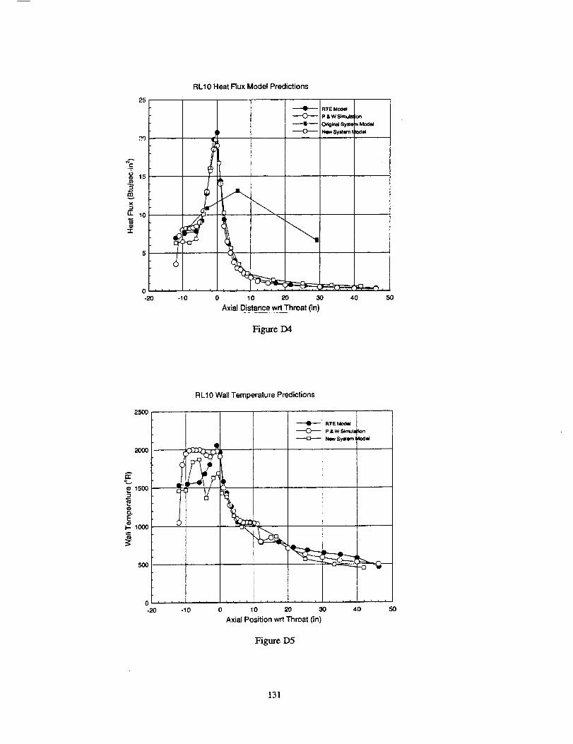
25

.'20

t""3"

15

gx

"7 10

-r-

RL1 0 Heat Rux Model Predictions

5 p

0-2o -I o 0

----91--- IRTE MoOe*I _ IP &w S;rnuldon

, _ IN_, Systern_

i xb i "---'

t_ ! '

10 20 3o 40 50

Axial Distance wrt Throat (in)

Figure D4

25OO

2OOO

Atr

15oo

IZ,

E

I.- 1000

RL1 0 Wall Temperature Predictions

50o

0 .... ' ' ' '

-20 -10

"-"0-- RTE MoOel

p& w Simuq

------O---- New System

10 20 30

Axial Position wrt Throat (in)

lion

irll Jill i,ih

4O 5O

Figure D5

131

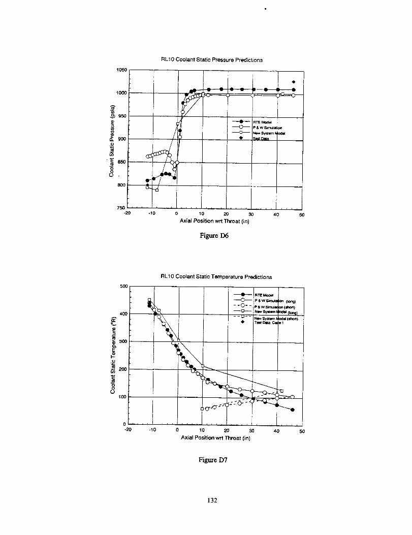
1050

1000

o}

950

co

_. 900

_85o-60

800

RL10 Coolant Static Pressure Predictions

ck.._

j_---__-_t_;3=== O

RTE Mode4

P & W Simula_ )n

New System _ IoOel

Tese Dala

750 ' ' ' ' ' • , , , I , , , , , , , , , , , .......

-20 -10 0 10 20 30 40 50

Axial Position wrt Throat (in)

Figure D6

5OO

4OO

300E

F-

200

_mOO

L_loo

o-20

RL10 Coolant Static Temperature Predictions

+ RTE MOdel

--O-- P &W_mu_ on (_oa)

r_\\ - - _- - _,, sy=,,. _L (=_o.)

_,_ qP Te_ DIla Ca;el

, L , , 7 , ...... i ,Ji , , , , • r ....

-10 0 10 20 30 40 50

Axial Position wrl Throat (in)

Figure D7

132

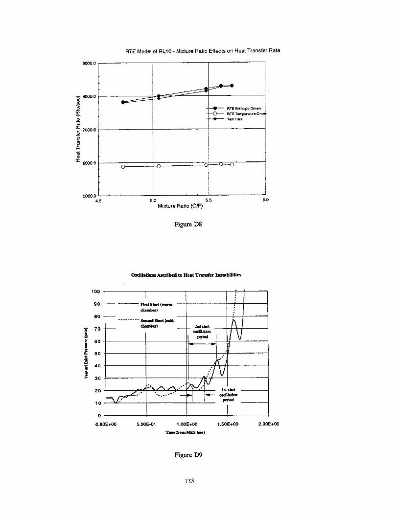
9000.0

-_ 8000.0

g

_ 7ol?o.o

e-

k-

-r"6000.0

5000.04.5

RTE Model of RLIO - Mixture Ratio Effects on Heat Transfer Rate

C_

, i

5.0

Mixture Ratio (O/F)

5.5

--O'---- RTE Enthoipy-Dnven

RTE Temperatuce- Driv_

Test Dela

i i

6.0

FigureD8

Oscillations Ascribed to Heat Transfer I_stablUties

A

o

1¢

100

90

80

70

60

50

40

30

20

lO

0

p

1lqnt Start (,mr*. --

chamber)

......... Sem_ St,rt(,_d

d,aae_) 2_d slmrt

es:matkm

t_ ....-o*

p

/vo*

S1= start

O.OOE+O0 5.00E-01 1.00E+O0

Item MF.S (=*¢)

1.50E+O0 2.00E+O0

Figure D9

133

APPENDIX E

Component Modeling of RL10 Injector, Combustion Chamber, and Nozzle

This appendix to the RL10A-3-3A Modeling Project Final Report describes efforts to predict theperformance of the RL10 propellant injectors, combustion chamber and nozzle using componentanalysis programs available to the NASA Lewis Research Center Space Propulsion TechnologyDivision (SPTD). A view of the combustion chamber and nozzle axial profile is shown in FigureEl. Cross-sectional views of the propellant injectors are shown in Figure E2.

E.1 Combustion Gas Property TablesThe CET93 program (Reference El) was used to calculate properties at each of fourteen axiallocations along the chamber and nozzle. These locations correspond to the heat transfer calculationnodes for the regenerative cooling jacket. CET93 is a one-dimensional equilibrium (ODE)

program, and includes effects not considered in a chemically 'frozen' expansion. Figure E1 showsthe location of the property nodes for the RL10 model; these axial locations and the corresponding

expansion ratios are listed in Table El.

CET93 was used to create tables of static pressure, temperature and Math Number at each axialnode for a wide range of assumed injector-face pressures, mixture ratios (O/F) and propellant inletmixture enthalpies. Tables for other required properties such as density, enthalpy, Mach Number,thermal conductivity, viscosity were compiled as functions of static pressure, temperature and O/F

at any given location. Where necessary, extrapolation and limit-logic has been imposed on thetables to maintain physically realistic results, primarily in cases of extreme condensation within theengine exhaust gases (low temperature, large expanston ratio, etc.).

These property tables have been encoded for use with the ROCETS simulation software and arearchived in the THERM3 library.

E.2 Nozzle Performance Analysis.Nozzle performance is represented in the system model by maps of characteristic velocity, specific

impulse, and discharge coefficient. Various analytic codes were used to predict these parametersfor the RL10 design. Consider the tables of ideal characteristic velocity (ciae_*) as predicted by

CET93. The ideal and actual characteristic velocities are related by the c*-efficiency (rio,).

C* = Cideal* * lqc*

Figure E3 shows a comparison of the ODE predictions with values specified by Pratt & Whitneyfor liquid-liquid injection. The points on the CET93 tables fall right on top of the suggested curvesfrom Pratt & Whimey. For gaseous fuel injected with liquid oxidizer, the points from CE'I93match the P&W curves for O/F values greater than 3, as shown in Figure E4; below that, there is asmall deviation. The RL10 start and shutdown transients are typically LOX-rich and only operatebelow an O/F of 4 for a short interval. The Pratt & Whitney curves are more computationally

efficient than the CET93 output tables because they use a correction for fuel enthalpy rather than

making enthalpy a third input variable in the cia_* property table. The Pratt & Whitney curvesalso provide greater resolution with respect to variations in mixture ratio, having many more O/Fdata points than the tables generated using CET93. Since the c* data provided by Pratt & Whitneywere verified using the ODE analysis, it was decided to continue using the provided ci_* curves

in the new system model. Efforts to predict the c*-efficiency are discussed in the section E.3below.

CET93 was also used to predict the ideal specific impulse (Isp)iOeal for the RL10 engine. Specific

impulse is used to predict engine thrust and overall efficiency. Rocket engine nozzle flows

135

typically involve significant losses due to two-dimensional, boundary layer, f'mite-rate chemistryeffects which are not included in ODE calculations as described above. These effects can be

estimated with tools which have been used extensively by engineers over the past thirty years. TheTDK (two-dimensional kinematics) program (Reference E2) used on the RL10 project is a standardand well-accepted tool for making such predictions. The actual specific impulse is related to theideal specific impulse by the expression

(Isp)n,x = (Isp)i_ * Tlcf* rio*

A table of thrnst-ooefficient efficiency (Hcf) was generated for the RL10A-3-3A based on TDK

output, and is shown in Table E3 and Figure E7.

Figure E8 shows a comparison of the predicted actual Isp (as calculated using the expressionabove) with the values specified by Pratt & Whitney. The figure portrays the variation in Isp asfunctions of O/F at different Pc values. As can be seen in the figure, the predicted and suggestedvalues match well, especially at pressures and mixture ratios near the RL10 engine's normaloperating condition (O/F = 5., Pc=475.). The predicted and suggested curves diverge from eachother at high and low mixture ratios, and there is a general disagreement between the two data setsat very low pressures. The Isp data set provided by Pratt & Whitney combines a table of idealvacuum Isp with simple empirical corrections for non-ideal effects. Although the range of pressureand mixture-ratio provided suggests that the tables can be used at very low pressures, theapplicable range of O/F is not clear. At very low pressures and very high mixture ratios, thesuggested empirical corrections may, in fact, predict negative Isp values (which is not reasonable).

After considering these issues, it was decided to use the rlcf tables predicted by TDK and the

(Isp)_ tables predicted by CET93 in the new system model.

Other analyses were done to estimate the nozzle discharge coefficient (C.a). A Navier-Stokes

analysis (Reference E3) was used to predict Cd at the engine's design conditions (Figure E5).From this analysis, the effective discharge coefficient of the nozzle was estimated to be 0.976.Another analysis was performed using a simple one-dimensional nozzle flow model and trimmingthe assumed Cd to match chamber pressure; this analysis gave 0.975. The TDK program was also

used to predict Cd at off-design conditions, scaled to match the Navier-Stokes prediction at the

design point. The off-design Cd values are shown in Table E2 and Figure E6. Variations in Cdwith Pc and O/F can be attributed to finite-rate kinetics and viscous effects. In this case, however,

we were unable to adequately explain some of the dramatic Cd variations predicted by TDK (atmixture ratios of 4 and 20, for example). The RL10A-3-3A has a silver throat insert that creates a

sharp edge, not typically used and difficult for TDK to model. Although preliminary enginesimulations using the variable nozzle Cd predictions showed virtually no differences withsimulations using constant Ca, it was ultimately decided not to include the variable Cd tables in the

new engine system model. A constant Cd value of 0.975 is used instead.

E.3 Combustion/Injector Performance AnalysisODE and TDK can be used to predict the performance of the chamber and nozzle given idealconditions at the injector. In reality, there are certain inefficiencies associated with the injector thatwill significantly effect the overall performance of the engine. The ROCCID program (Reference

FA) was used to predict these effects, which are represented by tic, (c-star efficiency) for use in theengine simulation. ROCCID also predicts the distribution of propellant mixture ratio across thechamber cross-section and the axial burning efficiency as well.

The RL10A-3-3A injector (see Figure E2) is rather complicated, involving several different injector

136

element designs. Most of the injector elements are co-axial, the hydrogen in injected throughannular orifices around each LOX element. The outer concentric row of elements, however, inject

hydrogen only (which will affect wall cooling). It is possible that some of the error encountered inthe heat transfer model (Appendix D) is due to not including this film cooling effect in thosepredictions. Except for the inner row, all of the coaxial elements have LOX flow swirlers. Thefaceplate of the injector is transpiration cooled by a small flow of hydrogen through a rigimeshmaterial.

Not all of the features in the RL10A-3-3A injector design could be modeled in the ROCCID.ROCCID models LOX swirling elements but assumes that the swi:r.1 i.s produced b.y injectin.g the

LOX tangentially through orifices. This is a more contemporary clesxgn man me nt_tmn-swmerelements actually used in the RL10A-3-3A. It was necessary, therefor, to consider the geometry ofthe ribbon swirlers and estimate an equivalent configuration for tangential flow injection. Thederivation of this estimate is shown in Figure E9. The estimates for orifice size had to be modified

subsequently to better match the overall pressure drop measured across the LOX elements.ROCCID also required some estimates of empirical factors and other equivalent design parametersnot known for the RL10. The faceplate transpiration cooling flow was not modeled for the RL10and the inner row of injector elements was considered identical to the other coaxial elements (i.e.

with LOX swirler elements).

Figure El0 shows the ROCCID predictions of overall rio, in the chamber as a function of mixtureratio and chamber pressure; the propellant inlet temperature assumed for the prediction is 300 R.

The figure also shows the values of rio* specified by Pratt & Whitney for the RL10A-3-3A, which

are presumed to be the results of test data. Comparison of the ROCCID predictions with the Pratt

& Whitney data shows significant differences. ROCCID predicts that the variation of tic* with

pressure will not be the same for all mixture ratios as is suggested by the Pratt & Whitney'scurves. The ROCCID analyses also indicate that there will be an appreciable variation in the c*-

efficiency with inlet fuel temperature, as illustrated in Figure Ell.

Significant uncertainty exists regarding the reliability of both the Pratt & Whitney data and the

ROCCID predictions. It should also be noted that the entire range of variation in rio. is only about4 to 8%; the differences between the predicted and P&W data may not be significantly larger than

the measurement accuracy of the test data or the numerical tolerance for the model. Neither _c* map

is considered an adequate representation of the combustion performance for start transientsimulations. The suggested performance curves from Pratt & Whitney lack any.considerations forvariation in fuel temperature, which is known to have a significant performance tmpact. On theother hand, model geometry alterations and persistent stability problems have adversely affect the

credibility of the ROCCID predictions. The decision was made to retain the tic, tables provided by

Pratt & Whitney in the new RL10 system model.

E.4 SummaryThe analyses performed for the RL10A-3-3A combustion chamber and nozzle have been useful inproviding insight into the behavior of these components. These modeling activities have also beenuseful in examining the application of various tools to existing rocket engine designs such as theRL10. Unfortunately, several of the analyses results did not verify the performance data provided

to us by Pratt & Whitney. Given the tight schedule imposed on these modeling attempts, it wasnot possible to make full use of the comparisons to modify the models or suggest more detailedinvestigations. Under these circumstances, it was decided that only the more detailed gas propertyand predicted specific impulse tables should be incorporated into the new system model. TheNavier-Stokes analysis of the nozzle throat also provided an excellent verification of the dischargecoefficient inferred from RL10A-3-3A test data.

137

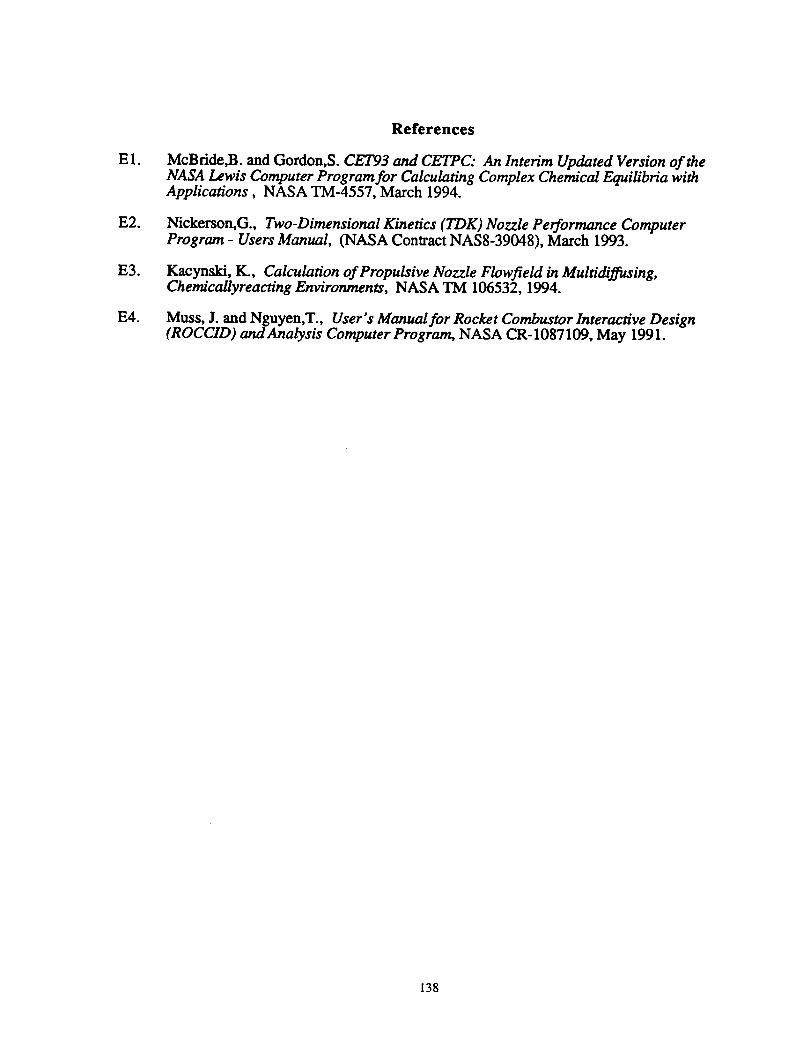
El.

E2.

E3.

E4.

References

McBride,B. and Gordon,S. CET93 and CETPC: An Interim Updated Version oftheNASA Lewis Computer Program for CalculatingComplex Chemical EquilibriawithApplications, NASA TM-4557, March 1994.

Nickerson,G., Two-Dimensional Kinetics (TDK) Nozzle Performance ComputerProgram - Users Manual, (NASA Contract NAS8-39048), March 1993.

Kacyns_, IC, Calculation of Propulsive Nozzle Flowfield in Multidiffusing,Chemicallyreacting Environments, NASA TM 106532, 1994.

Muss, J. and Nguyen,T., User's Manual for Rocket Combustor Interactive Design(ROCCID) and Analysis Computer Program, NASA CR-1087109, May 1991.

138

Table E1

Hot-Gas Property NodeAxial Locations and Expansion Ratios for

NASA LeRC Model of RL10A-3-3A

Axial Location

(inches wrt throat)

-0.500

0.485

-2.018

2.035

-4.054 2.72

Expansion Ratios(wrt throat)

1.11 subsonic

1.29 supersonic

1.62 subsonic

2.35 supersonic

subsonic

-6.068

-8.032

-10.00

-12.00

4.215

6.588

8.989

16.54

25.05

33.41

41.84 56.1

3.65 subsonic

4.00 subsonic

4.14 subsonic

4.27 subsonic

4.29 supersonic

6.93 supersonic

9.95 supersonic

20.7 supersonic

33.2 supersonic

45.0 supersonic

supersonic

O/F=I

O/F=4

O/F=6

O/F=8

O/F=10

O/F=20

O/F=50

Table E2

TDK Predicted Discharge Coefficients for

Pc=5 psia

0.973

1.011

1.008

1.005

1.005

1.016

0.979

RL10A.3-3A

Pc=50 psia

0.975

0.988

0.983

0.981

0.981

O.987

0.978

Nozzle

Pc=150 psia

0.975

0.971

0.976

0.975

0.975

0.989

0.978

Pc=500

0.976

0.977

0.975

0.974

0.974

0.975

0.977

139

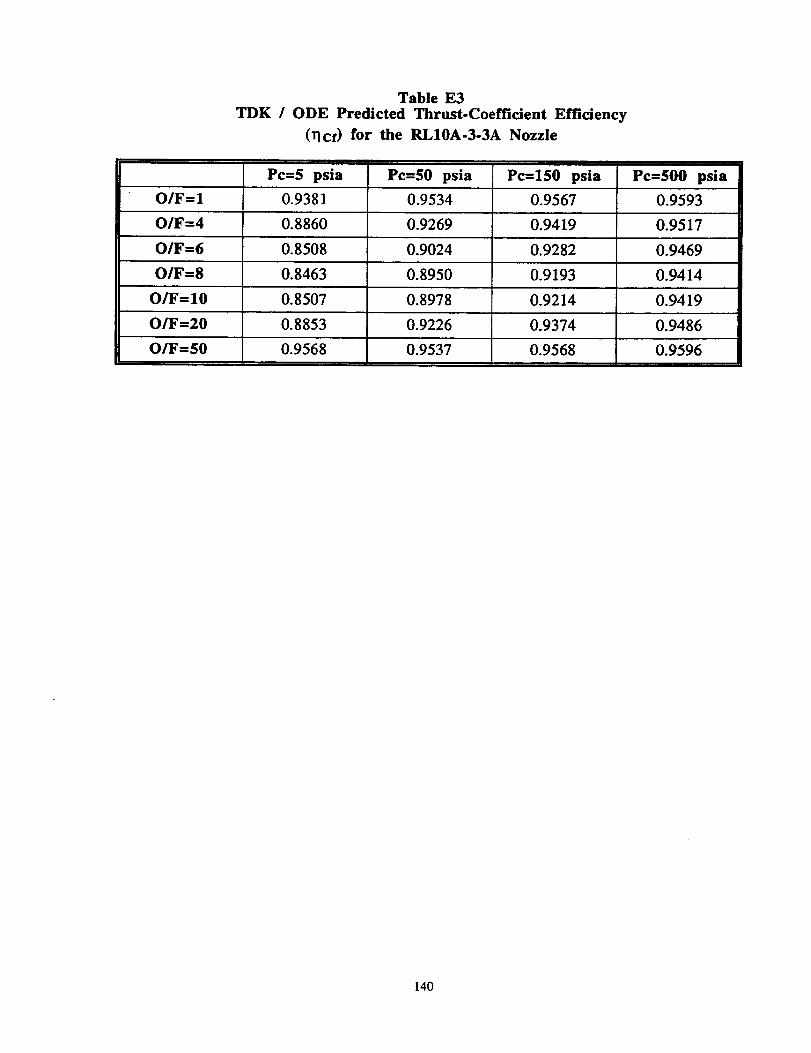
Table E3

TDK / ODE Predicted Thrust-Coefficient Efficiency

(_cf) for the RL10A-3-3A Nozzle

Pc=5 psia Pc=50 psia Pc=150 psia Pc=500 psia

O/F= 1 0.9381 0.9534 0.9567 0.9593

O/F=4 0.8860 0.9269 0.9419 0.9517

O/F=6 0.8508 0.9024 0.9282 0.9469

O/F=8 0.8463 0.8950 0.9193 0.9414

O/F= 10 0.8507 0.8978 0.9214 0.9419

O/F=20 0.8853 0.9226 0.9374 0.9486

O/F=50 0.9568 0.9537 0.9568 0.9596

140

Chamber and Nozzle Prorde with property Node LocaUons

4

Z

0

-15

I

III

!

Ii

-5 5 15 Z5 35 45 SS

TubeProfile

Cast SilverThroatInsert

Detail of Throat (notto=_=)

Figure E1

141

LOX

Ignitor

Fuel LOX InjectorPlennum

Suppo_Boss

Detail of _plml InjectorElement

Fuel InjectorPlennum

CombustionChamber

LOX Plennum rBulkhead

_\\\\\\\\_\\\_, \\\\\_

_" SwIHer

RigimuhFlaceplat¢

Figure E2

142

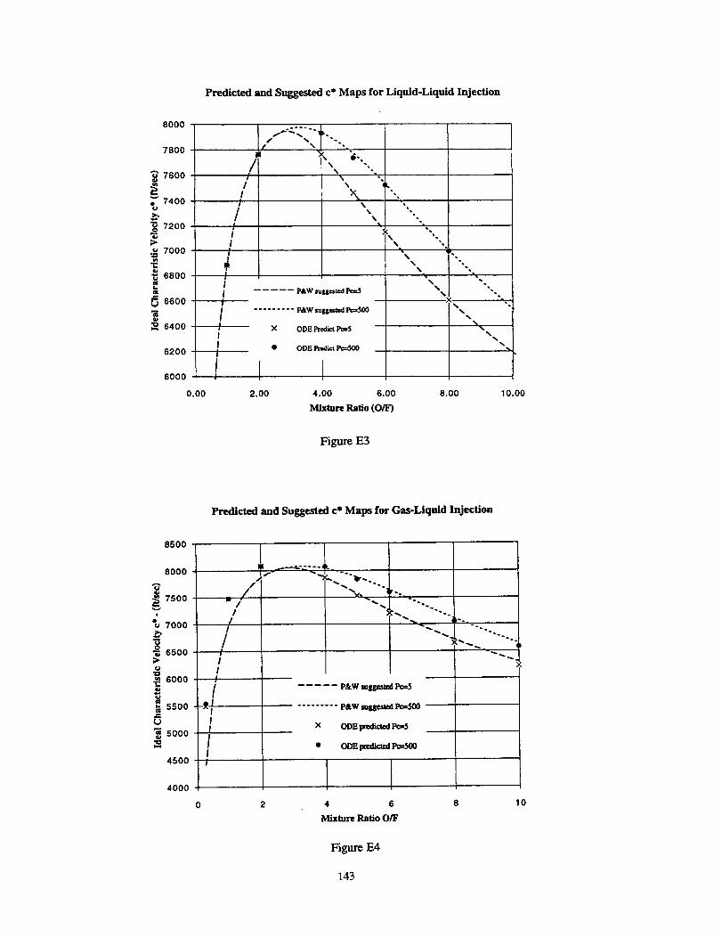
Predicted and Suggested c* Maps for Liquid-Liquid Injection

8000

7800

/"_ 7600 /

. 7400 /

"_ 7200 I"_ I

I

7000 I

6800 II

6600 ----r--

6400 ----+--II

6200 ----1--

6000 !

o.oo

/

_\ d-.\

s\

x,\

%

..... P&W suggested P_-,5

......... P&W suggezted Pc=500

X ODE Predict P_--5 --

• ODE Predict P_---500 __

I,

i

•=

%%

%

%

%

% *.

%% ".

X m%

%.

%.,.%.

"%%

%

2.00 4.00 6.00 8.00

Mixture Ratio (O/F)

10.00

Figure E3

Predicted and Suggested c* Maps for Gas-Liquid Injection

8500

8000

_,,_=_7500i

7000

_6500

6000

55oo

5ooo

4500

4000

- ./

!/

I

/III

I

/

X

_('a r-.=

...... P&Wmggested

P&Wmgg--_d Po,500

ODE_ Po-5

ODEpledicu:dPc=500

,-o

4 6

Mixture Ratio O/F

Figure E4

lO

143

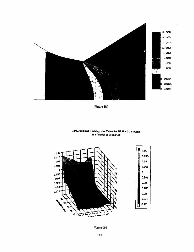
FigureE5

TDK Predicted Discharge Coefficient for RL10A-3-3A Nozzle

as a function of Pc and O/F

1.01

1

0.99"

0.98

0.975

1.02

1.015

1.01

1.005

I

3.995

:).99

:).985

:).98

).975

).97

Figure E6

144

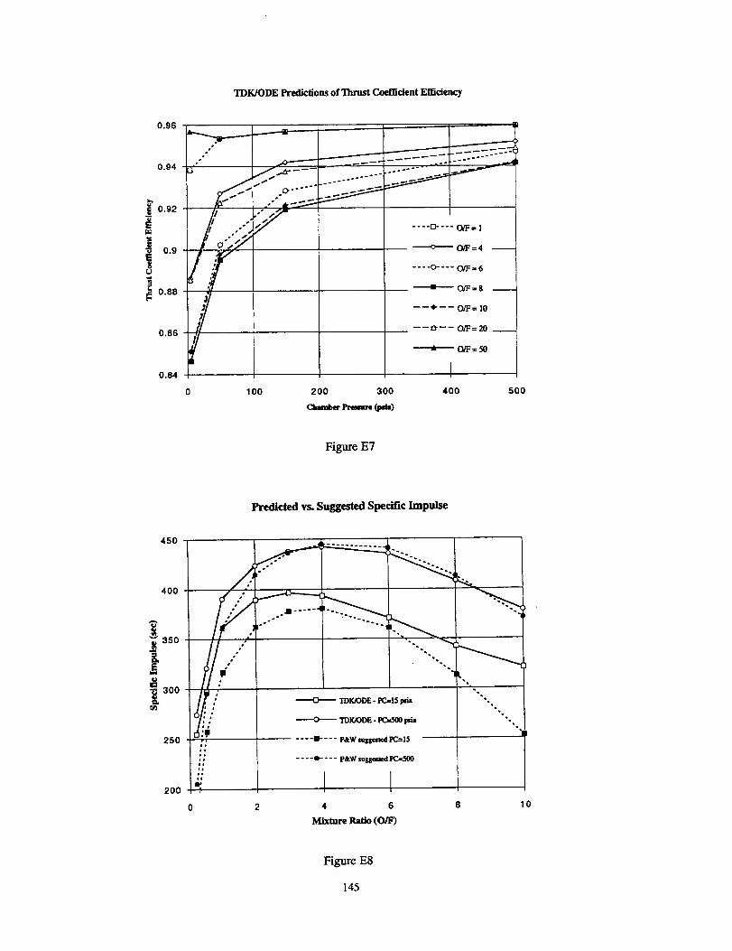
TDK/ODE Predictions of Thrust Coefficient Emciency

0.96

0.94

_' 0.92

i 0.9

_ 0.88

0.86

0.84

.°o

_1,°

/100 200 300

_Pre,=e.e(pa=)

..... -.-- ..........

.... ET---- O/F=I

----O-'--- O/F=4

.... O---- O/F=6

O/F=$

----_'--- O/F= 10

----_'--- O/F= 20

O/F= 50

I

400 500

Figure E7

Predicted vs. Suggested Specific Impulse

450

400

'_ 350

3OO

250

20O

J

,o

Ii

H

e:.

toO-'--- IDK/ODE - PC=IS pei= ""%'%

---o---- TDIOODE- PC,,,500_ ..

.... B-- - - P&W SUggested !_..= 15

.... • .... P&W mUaaxl

2 4 6 8

MixtureRatio(O/F)

10

Figure E8

145

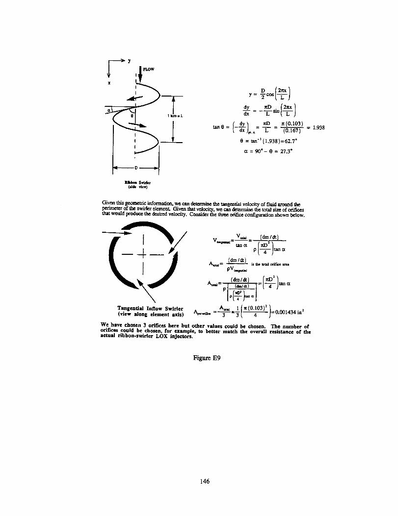
Y FLOW

_---- 0 ------_

(d(k 'dew)

D (2_ Iy= "-_cos I-'-_- j

dy _rD ( 2zx 1

d_ _ ---L-_(-'L-)

I dy) = _.D = _(0.103)ran0 = -'_'x _^ --L- (0.167)

0 = tan-_(1.938)=62.7"

a = 90 °- 0 = 27.3"

= 1.938

Given this geometric information, we can de_rmine the tangential velocity of fluid around

_t_._.of _. sw@._el_._,,)._,_t v_o_ty,we_ de_=al_ _ to_ si= ofo_c_woma proauce me desired velocity.Consider the lhrec orificeconfigurationshown below.

Tangential Inflow Swirler

(view along element axis)

v_ (dm/d0Vmq_.,., =-- =

tana rd_) 2°/T)-°_= _ ist_t_l_'i/kelma

PV_v._

_D 2

(¢,n/dt) __[T)mnaA_= _ I {'--/dO

A_,., I (_(0.I03) 2 ] ...... ,

A,__.=-T-=-_l -_ /--u._,,_,,n

We have chosen 3 orifices here but other values could be chosen. The number oforifices could be chosen, for example, to better match the overall resistance of theactual rihbon-swirler LOX injectors.

Figure E9

146

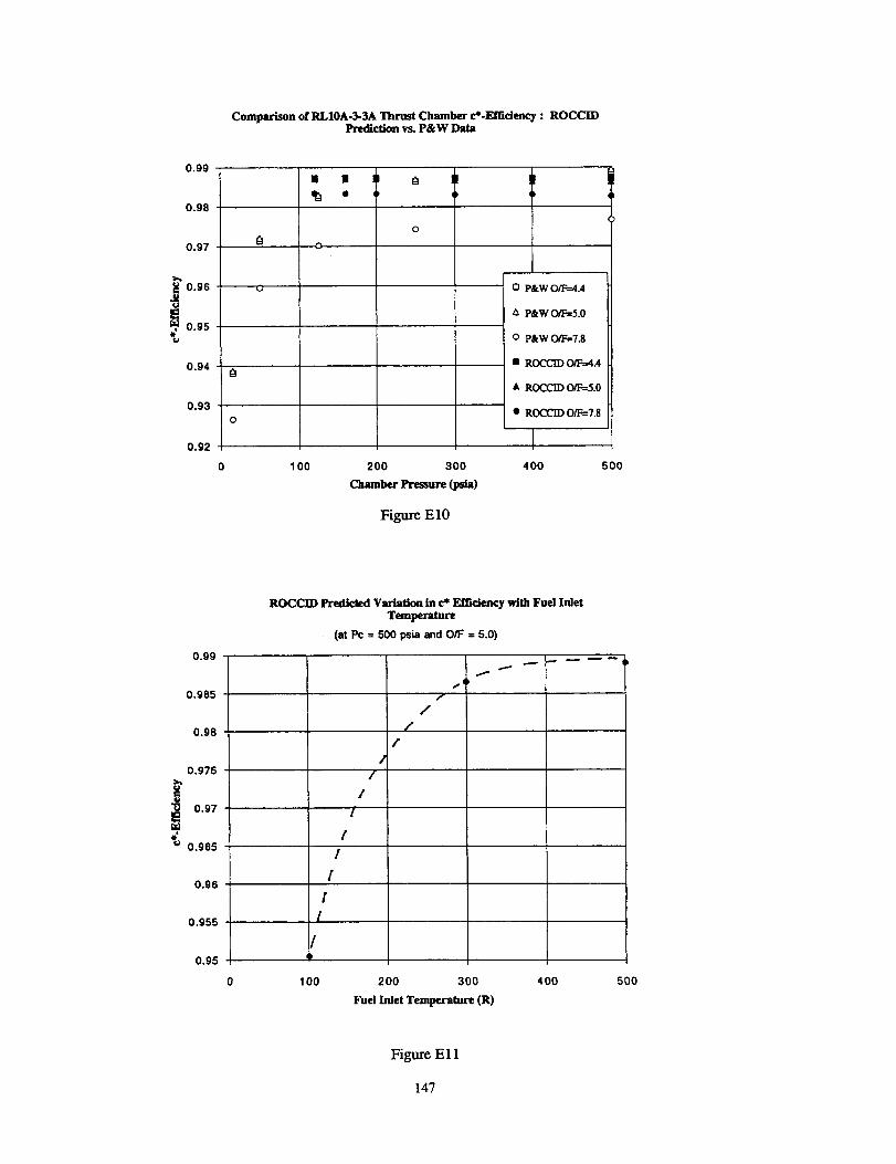
Comparison of RLIOA-3-3A Thrust Chamber c*-Efllciency : ROCCIDPrediction vs. P&W Data

0.99

0.98

0.97

F_o96"0

_, o.95

0.94

0.93

0.92

@

0

D P&W O/Ff4A

A P&W O/F'=5.O

O P&W O/F=7.8

• ROCCID O/I:=4.4

• ROCCID O/F=-5.0

• ROCCID O/F=7.8

1O0 200 300 400

ChamberPressure(psta)

Figure EIO

500

0.99

0.985

0.98

0.975>.b

"0 0.97

0.965

0.96

0.955

0.95

ROCCID Predicted Variation in c* Eflldency with Fuel Inlet

Temperature

(at Pc = 500 psia and 0/!: = 5.0)

/

/

/

//

I

li

/,/

/

,,,.(

f

100 200 300

Fuel Inlet Temperature (R)

400 500

Figure E11

147

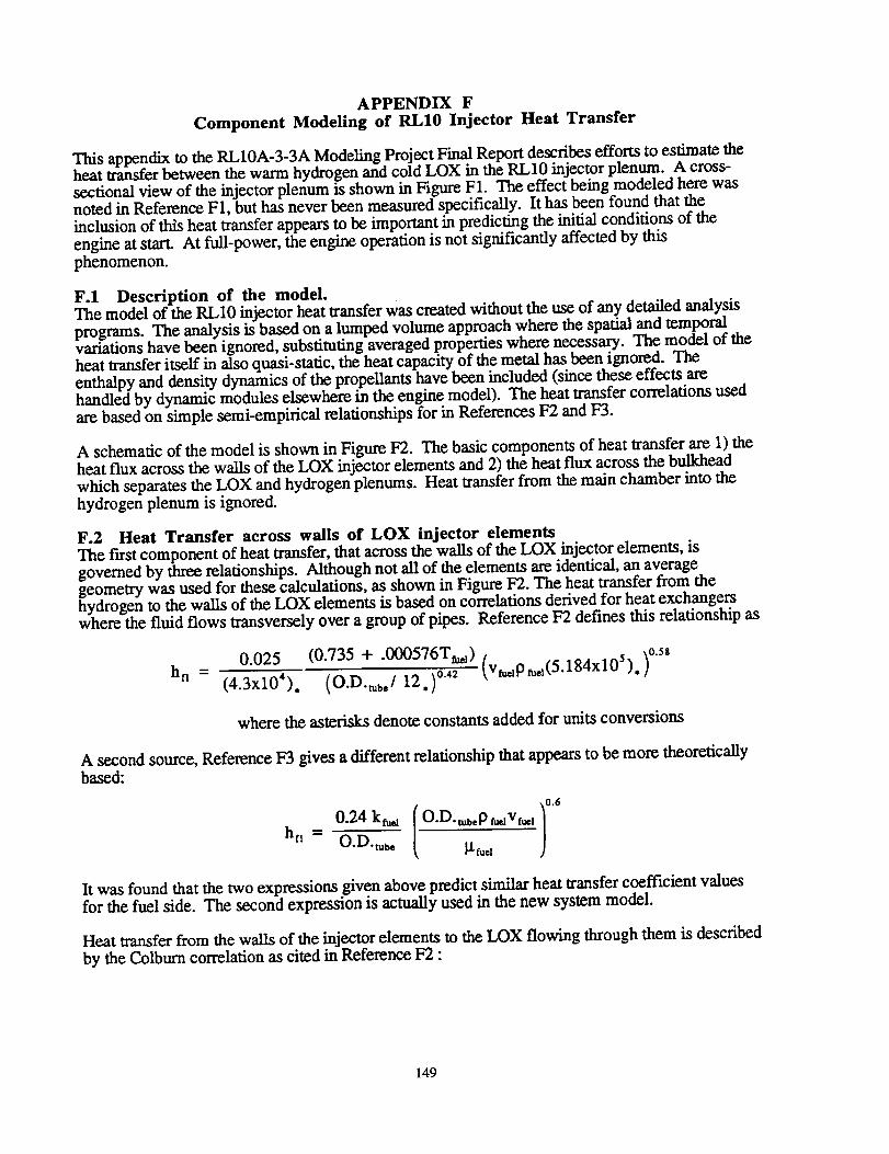
APPENDIX F

Component Modeling of RL10 Injector Heat Transfer

This appendix to the RL10A-3-3A Modeling Project Final Report describes efforts to estimate theheat transfer between the warm hydrogen and cold LOX in the RL10 injector plenum. A cross-sectional view of the injector plenum is shown in Figure F1. The effect being modeled here wasnoted in Reference F1, but has never been measured specifically. It has been found that theinclusion of this heat transfer appears to be important in predicting the initial conditions of the

engine at start. At full-power, the engine operation is not significantly affected by this

phenomenon.

F.1 Description of the model.The model of the RLIO injector heat transfer Was created without the use of any detailed analysis

programs. The analysis is based on a lumped volume approach where the spatial and temporalvariations have been ignored, substituting averaged properties where necessary. The model of theheat transfer itself in also quasi-static, the heat capacity of the metal has been ignored. The

enthalpy and density dynamics of the propellants have been included (since these effects arehandled by dynamic modules elsewhere in the engine model). The heat transfer correlations usedare based on simple semi-empirical relationships for in References F2 and F3.

A schematic of the model is shown in Figure F2. The basic components of heat transfer are 1) theheat flux across the walls of the LOX injector elements and 2) the heat flux across the bulkhead

which separates the LOX and hydrogen plenums. Heat transfer from the main chamber into the

hydrogen plenum is ignored.

F.2 Heat Transfer across walls of LOX injector elements

The fzrst component of heat transfer, that across the walls of the LOX injector elements, isgoverned by three relationships. Although not all of the elements are identical, an averagegeometry was used for these calculations, as shown in Figure F2. The heat transfer from thehydrogen to the walls of the LOX elements is based on correlations derived for heat exchangerswhere the fluid flows transversely over a group of pipes. Reference F2 defines this relationship as

0.025 (0.735 + .000576T_,a) (vr_,apf_a(5.184x105).)°-5'hn (4.3x10'). (O.D.mb, / 12.)"

where the asterisks denote constants added for units conversions

A second source, Reference F3 gives a different relationship that appears to be more theoretically

based:

hfl -

0.24 kfu,a

O.D. tube

It was found that the two expressions given above predict similar heat transfer coefficient valuesfor the fuel side. The second expression is actually used in the new system model.

Heat transfer from the walls of the injector elements to the LOX flowing through them is described

by the Colbum correlation as cited in Reference F2"

149

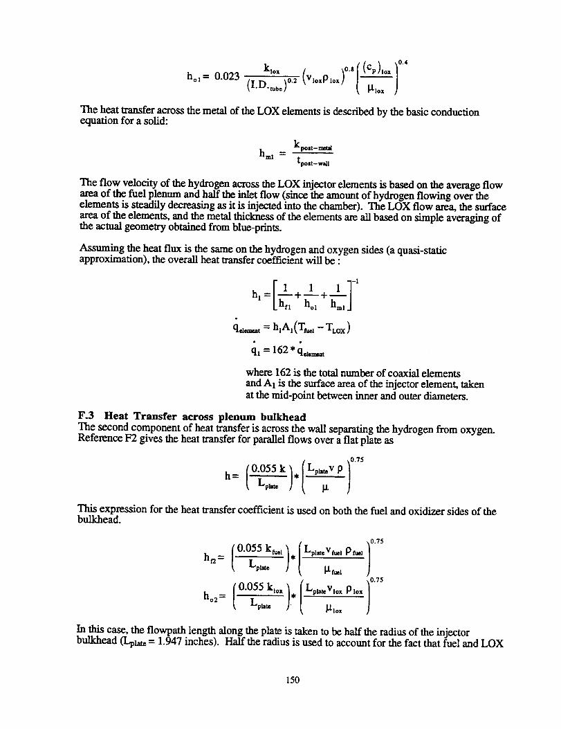
hol= 0.023 k'°" (VloxPlox) °'s(I.D._.) °'2

The heat transfer across the metal of the LOX elements is described by the basic conductionequation for a solid:

k post - rental

hml

tpost-w_ll

The flow velocity of the hydrogen across the LOX injector elements is based on the average flowarea of the fuel plenum and half the inlet flow (since the mount of hydrogen flowing over theelements is steadily decreasing as it is injected into the chamber). The LOX flow area, the surfacearea of the elements, and the metal thickness of the elements are all based on simple averaging ofthe actual geometry obtained from blue-prints.

Assuming the heat flux is the same on the hydrogen and oxygen sides (a quasi-staticapproximation), the overall heat transfer coefficient will be"

1 1+11-1

q_H = h,A,(T_ - TLox)

ql = 162" a,mt

where 162 is the total number of coaxial elements

and A1 is the surface area of the injector element, takenat the mid-point between inner and outer diameters.

F.3 Heat Transfer across plenum bulkhead

The second component of heat transfer is across the wall separating the hydrogen from oxygen.Reference F2 gives the heat transfer for parallel flows over a flat plate as

h_

This expression for the heat transfer coefficient is used on both the fuel and oxidizer sides of thebulkhead.

hn= (0"055 kt_e' ) *Lp,ate

ho2 = (0.055Lp latekl° x ),

LplateVfuel P ft_.l

lj" fuel

LplateVlox P fox

_'_lox

0.75

).75

In this case, the flowpath length along the plate is taken to be half the radius of the injectorbulkhead (Lplm = 1.947 inches). Half the radius is used to account for the fact that fuel and LOX

150

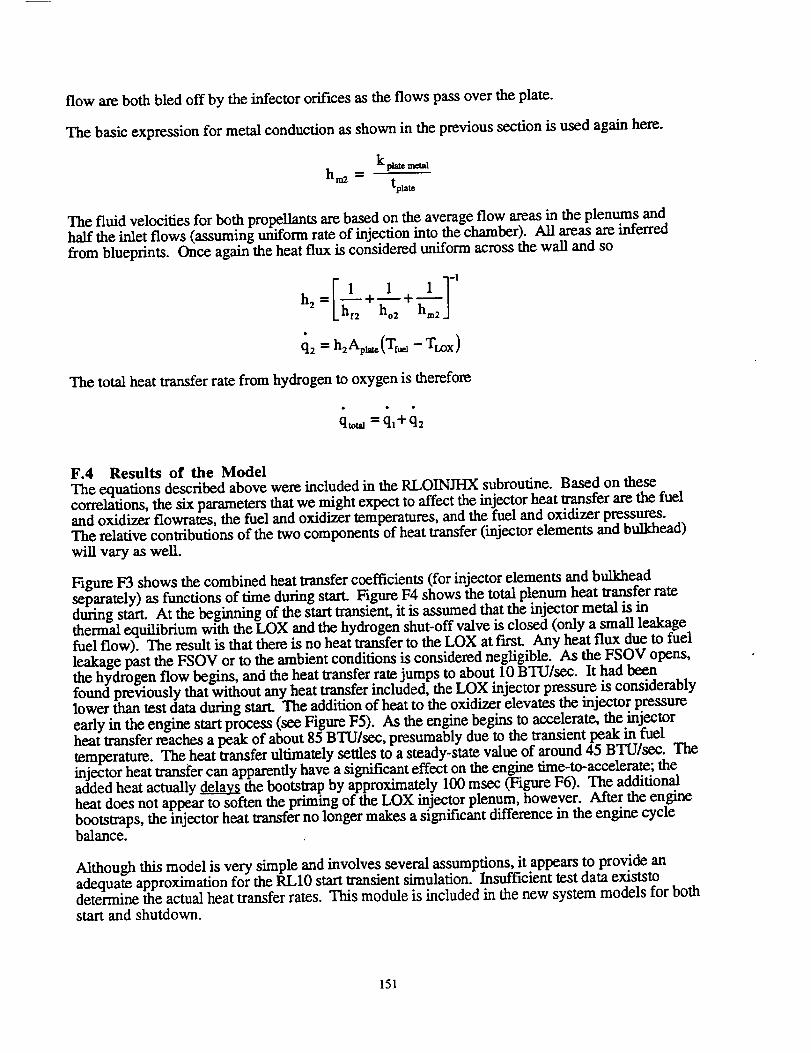
flow are both bled off by the infector orifices as the flows pass over the plate.

The basic expression for metal conduction as shown in the previous section is used again here.

The fluid velocities for both propellants are based on the average flow areas in the plenums andhalf the inlet flows (assuming uniform rate of injection into the chamber). All areas are inferred

from blueprints. Once again the heat flux is considered uniform across the wall and so

I 1 1-11 +_.._1+

q: = h2Ap_(Trm - Tu_x)

The total heat transfer rate from hydrogen to oxygen is therefore

q_ = q_+ q2

F.4 Results of the ModelThe equations described above were included in the RLOINJHX subroutine. Based on thesecorrelations, the six parameters that we might expect to affect the injector heat transfer are the fueland oxidizer flowrates, the fuel and oxidizer temperatures, and the fuel and oxidizer pressures.The relative contributions of the two components of heat transfer (injector elements and bulkhead)

will vary as well.

Figure F3 shows the combined heat transfer coefficients (for injector elements and bulkheadseparately) as functions of time during start. Figure F4 shows the total plenum heat transfer rateduring start. At the beginning of the start wansient, it is assumed that the injector metal is inthermal equilibrium with the LOX and the hydrogen shut-off valve is closed (only a small leakagefuel flow). The result is that there is no heat transfer to the LOX at first. Any heat flux due to fuelleakage past the FSOV or to the ambient conditions is considered negligible. As the FSOV opens,the hydrogen flow begins, and the heat transfer rate jumps to about 10 BTU/sec. It had beenfound previously that without any heat transfer included, the LOX injector pressure is considerablylower than test data during start. The addition of heat to the oxidizer elevates the injector pressure

early in the engine start process (see Figure F5). As the engine begins to accelerate, the injectorheat transfer reaches a peak of about 85 BTU/sec, presumably due to the transient peak in fuel

temperature. The heat transfer ultimately settles to a steady-state value of around 45 BTU/sec. Theinjector heat transfer can apparently have a significant effect on the engine l_ne-to-accelerate; theadded heat actually de_g!a_ the bootstrap by approximately 100 msec (Figure F6). The additionalheat does not appear to soften the priming of the LOX injector plenum, however. After the enginebootstraps, the injector heat transfer no longer makes a significant difference in the engine cyclebalance.

Although this model is very simple and involves several assumptions, it appears to provide anadequate approximation for the RL10 start transient simulation. Insufficient test data existstodetermine the actual heat transfer rates. This module is included in the new system models for both

start and shutdown.

151

F1.

References

Wanhainen, R., Throttling Characteristics of a Hydrogen-Oxygen, Regeneratively Cooled,Pump-Fed Rocket Engine, NASA TM X-1043, December 1964.

Brown,A. and Maxco,S., Introduction to Heat Transfer, McGraw Hill, New York 1951.

Faires,V., Applied Thermodynamics, MacMillan Company, New York 1947.

152

LOX

Ignitor

FuelSupport

LOXInjector BoasPlennum

\

Dud I_jcctorPlennum

Combustion

Chamber

Figure F1

Detail of Typical InjectorElement

LOX Plennum

/ •RigtmeshFlaceplate

wider

Heat transfer

defined by axialflow throu

pipe.

Fuel Injector- Plennum

CHAMBER

Figure F2

153

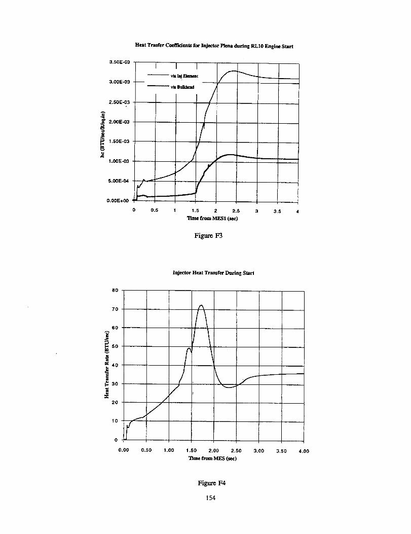
3.50E-03

3._E-03

2.50E-_

i 2.00E-03

1.50E-03

1.00E-_

5._E-_

O.OOE+_

Heat Trasfer Coeflidents for Injector Plena during RLI0 Engine Start

I

I I

_" via Bul_ead

I

0.5 1 1.5 2 2.5

Time fromIVIES](see)3.5

Figure F3

8O

Injector Heat Transfer During Start

7O

60

_omv

40

¢1

30

2O

10t

0.00 0.50 1.00 1.50 2.00 2.50

Time from MES (sec)

3.00 3.50 4.00

Figure F4

154

Heat Transfer Effects on LOX Injector Plenum Pressure Early in RL10

Engine Start

3O

28

._,26

_24Z

22

20

0 14=.1

12

10

LWith Heat X-fer --

w/o Heat X-fer __

Jf

/J

0.00 0.20 0.40 0.60 0.80

Time from MES1 (sec)

Figure F5

1.00

Heat Transfer Effects on Bootstrap Time during RLI0 Engine Start

700

6OO

_,_ 500

I_ 400

Et=

E 300

_' 200

C,J

100

With Heat X-ler

-- wlo Heat X-fer

( - 100 msec difference )

Y0.00 0.50 1.00

3[3me from MF_,SI (sec)

Figure F6

1.50 2.00

155

APPENDIX G

Component Modeling of RL10 Duct Flow

Duct or manifold flow-resistence is typically established by test. Pratt & Whitney provided us withflow-resistences based on such tests for the RL10 engine. The resistence values specified were

typically 'lumped', with several sections of ductwork combined into a single resistence. Our goalin this project was not to replace the P&W values but to benchmark the accuracy of simple one-dimensional flow models against the P&W resistences. If the models showed promise, they could

be used to predict the effects of design changes in the RL10, and to predict the resistences of ductsand manifolds in new engine designs. Toward that end, we selected a single flow-resistence fromthe P&W data, one which could be clearly identified with a single physical component in the

engine.

The duct chosen was that from the turbine housing discharge to the main fuel shut off valve. This

duct is shown in Figure G1. The analysis performed was a based on Darcy's formula forcompressibile flow. The analysis was done both manually and using the Crane software asdescribed in References G 1 and G2. The solution is complicated because of the large number of

non-90-degree bends and the fact that the friction factor for the duct material is not known.

It should be noted that friction losses were also calculated by the RTE code using similar methods

for the cooling jacket tubes. In that case, there are no discrete bends but the tubes are curved alongtheir entire length. RTE calculates losses due to the curvature using a semi-empirical correlation(see Reference G3). It is not known how accurate the RTE prediction is, although one estimate oferror could be set at about 6%. Further discussion of the prediction of cooling tube losses is not

given here.

G.1 Estimates of duct segment equivalent lengthsThe duct in question was decomposed into a series of curved and straight sections, as shown inFigure G1. Although the segments do not lie in a plane, any three-dimensional effects whichmight exist are not considered. Based on the angle of the bend, the radius of the bend, and aconstant duct diameter assumed to be 2.402 inches, the bends were modeled as an 'equivalent'

length in straight pipe. This is done automatically by the Crane software (probably by proratingthe bend angle from 90 degrees). Table G1 shows the equivalent lengths estimated by the programfor the bends in the duct.

Adding up the equivalent lengths of the bends and the straight section lengths, we obtain an overequivalent length of 123.8 inches, or 51.5 times the diameter of the pipe.

G.2 Determination of Pipe K factorThe friction losses in a pipe are often described by a K-factor, as defined by the equation below

m=A*Y- */kP pw42g *

In this expression for mass flow, Y is an expansion factor (used only for compressible flows), ZkP

is the pressure difference across the pipe, p is the density and g is the gravitational constant. K is

determined by the expression

fLK-

D

where f is the friction factor, L is the equivalent length, and D is the pipe inner diameter, f is not

157

known precisely and is often determined empirically for any given material and surface finish.Generally, the smoothest commercial pipe will have a friction factor (f) of at least 0.018. Theductwork of the RLIO is not, of course, commercial pipe. The friction factor is determined by thesurface roughness and the fluid Reynold's Number (which gives an indication of its viscosity anddegree of turbulence). A second estimate for the friction coefficient (f) of the duct may be obtained

by using an absolute roughness similar to that of the cooling jacket tubes (4.6xl0-Sinches), forexample. The friction factor would then be 0.0095 for complefly turbulent flow. Using these twovalues of f for commercial pipe and jacket tubing as upper and lower bounds, the predicted K forthe duct would be between 0.928 and 0.487.

G.3 Comparison of Prediction with suggested value.Pratt & Whimey has specified that the flow though this duct be modeled by the expression

m= • Ti,_

and Kc=0.4335 as suggested byPratt & Whitney.

This formula was probably empirically determined. This representation can be converted to theDarcy equation if we assume an ideal gas correlation for the hydrogen, modified by thecompressibility

Then K can be expressed by

K = Kc*(2g/R * A2*y 2)

If the expansion factor Y is assumed to be 0.931 (as predicted by the Crane software), then we seethat the suggested value of K is 0.648.

The predicted range of K values (0.487 to 0.928) encompasses the value specified by Pratt &Whitney. The predicted range of values includes uncertainty in the friction coefficient, f, and in theproper equivalent lengths for all the duct bends.

It might be possible to calibrate the ffor the RL10 ducts using the value of Kc provided by P&Wand described above. If necessary, this value could be used in conjunction with simple 1D modelsto predict the effect of changes to the RL10 ductwork. For new engine designs, there will be someuncertainty regarding the duct interior surface roughness. One dimensional models such as wereused here can be used to predict the flow-resistence with uncertainty for new designs. Two andthree dimensional flow analysis tools might also be used to refine estimates of flow resistence,especially in predicting the losses due to bends, flanges and other features. Tools of this kind aretypically complicated and difficult to use, and were considered beyond the scope of this project.The best method is still to use test data when available.

158

G1.

G2.

G3.

References

Crane Company, Technical Paper No. 410, Flow of Fluids Through Valves, Fittings, and

Pipe, 1982.

Crane Co. and ABZ Inc., Crane Companion to Flow of Fluids Through Valves, Fittings,

andPipe, (software), 1992.

Naraghi, M.H.N., RTE - A Computer Code for Three-Dimensional Rocket ThermalEvaluation, (NASA Grant NAG 3-892), July 1991.

159

Table G1

Estimated Equivalent Lengths of Duct Sections

Description Manual Estimate (in.)

0.185 in. straight section 0.185

97.5 deg.bend (R=3.75 in.) 35.21

2.825 in. straight section 2.825

67.5deg.bend (R=12 in.) 33.36

1.519 in. straight section 1.519

104.5 deg.bend (R=6.25 in.) 30.63

6.452 in. straight section

Software Estimate

0.185

34.8

2.825

28.80

1.519

32.40

3.572 in. straight section 3.572 3.572

30 deg.bend (R=10 in.) 5.212 13.20

6.452

Total

6.452

119.0n

*Actual length of the duct is approximately 51.7 inches.

123.8

(in.)

160

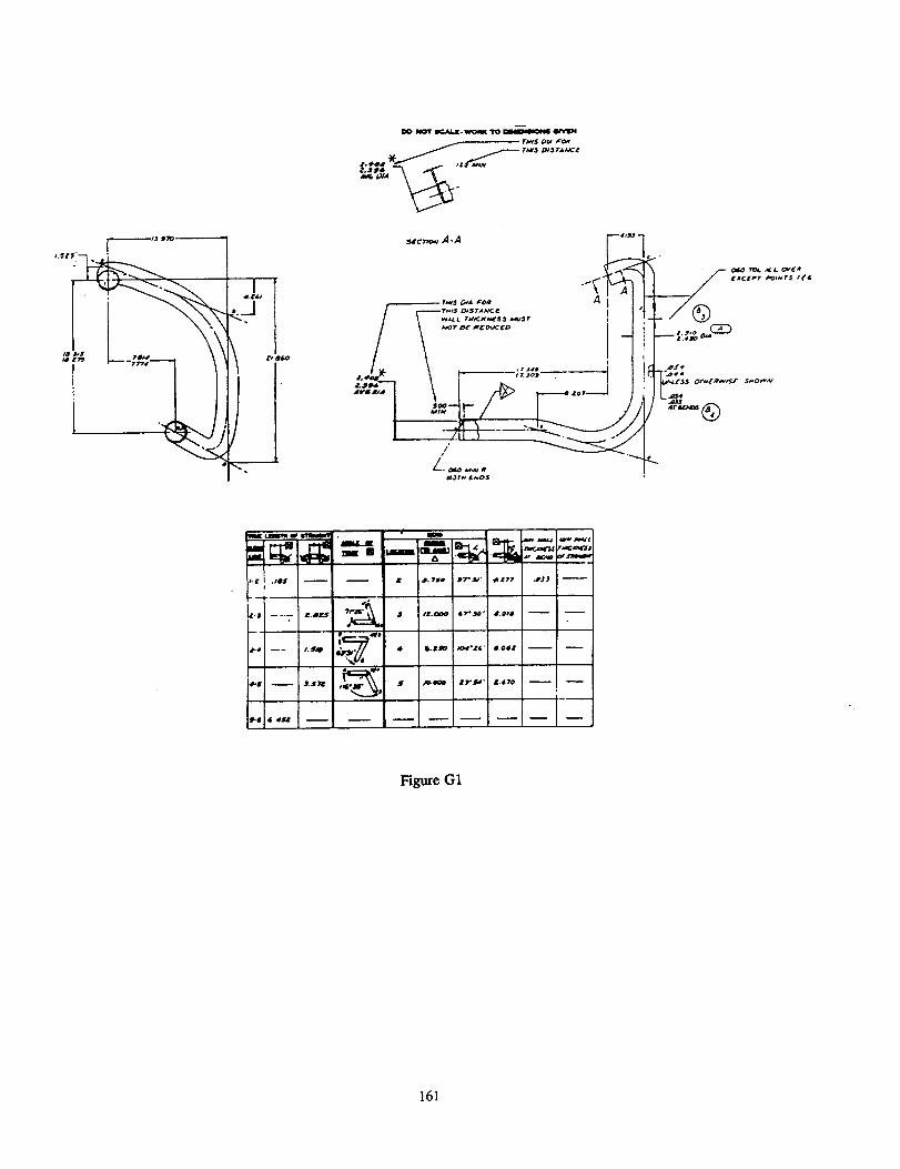
.?2

_ t_ _-TT'r4

_ No.t r._.z . w_ Iro _ #L_nrN

TN:$ _ Few

a- C . ¢_11" • J, ?SO J*7* ._* _ • T7 .0$ 3

J-d --_ l_tf_ 4 6-£J_ _°,f6 _ 4_-06_ '

Figure G1

161

APPENDIX H

Modeling of Two-Phase (Liquid/Gas) Flow

The RL10A-3-3A rocket engine experiences two-phase liquid-gas flow at several locations duringstart and shutdown transients. These locations include the pump volute tongues, fuel-pump cool-down valves, oxidizer control valve, LOX injector elements, and combustion chamber throat. Amodel of this behavior in required which includes the transition between choked and unchoked

flow, and the transition between single and two-phase flows.

H.1 Research performed regarding two-phase flowThere is a great deal of documentation on two-phase flow available (see references list).Unfortunately, much of this information is not applicable to rocket engine modeling. Many of thestudies are strictly for water-steam flows (where most of the industrial interest lies) and containempirical factors that don't necessarily apply to other fluids. Other research has been performed toinvestigate the physics of two-phase flow but has not produced useable correlations to predict theflow quantitatively. Still other correlations exist which are adequate for describing the flow in oneregime (choked or tmchoked, liquid, gas, or a two-phase mixture), but these expressions areincapable of estimating the transition between different behaviors. There are also several modelswhich, although general, are so complex and computationaUy intensive that they proved to bebeyond the scope of this project to incorporate. The approach that has been taken to model two-phase flow in the RL10 is based on several research papers (References H4 to H7). In somecases, the correlations suggested by this research have been replaced with simplified expressions

and the transitions predicted by averaging the gas and liquid flow predictions.

H.2 Heterogenous fluid approachesHeterogenous models keep the liquid and gas components of the two-phase mixture separate anddistinct. The velocity of the gas bubbles is considered, as well as interactions (phase transitions)between the liquid and gas components caused by pressure and temperature variations along the

path of the fluid. This can lead to a rather complex set of equations that must be solvedsimultaneously.

One such description of two-phase flow in short tubes, nozzles, and orifices is presented inReference H4. In order to create such a heterogenous model, many estimates and assumptions

pertaining to bubble formation and velocity, interphase mass and energy transfer, etc. arerequired. We were unable to reliably estimate such parameters for the RL10 components. It wastherefore decided to focus on homogenous models instead, and return to the study of heterogenous

models only if necessary. No further work was done on heterogenous models for the RL10

project.

H.3 Homogenous fluid approachesHomogenous models treat the two-phase mixture as a single phase fluid with averaged properties.A number of different homogenous models have also been proposed (References H1 to H3), but

most are based on empirical data and may not be applicable to cryogenic fluids. One relativelygeneral approach is described in References H5 and H6. This method assumes isentropic flowthrough an orifice and can be used for both choked and unchoked flow. The expression for massflux in this model is

163

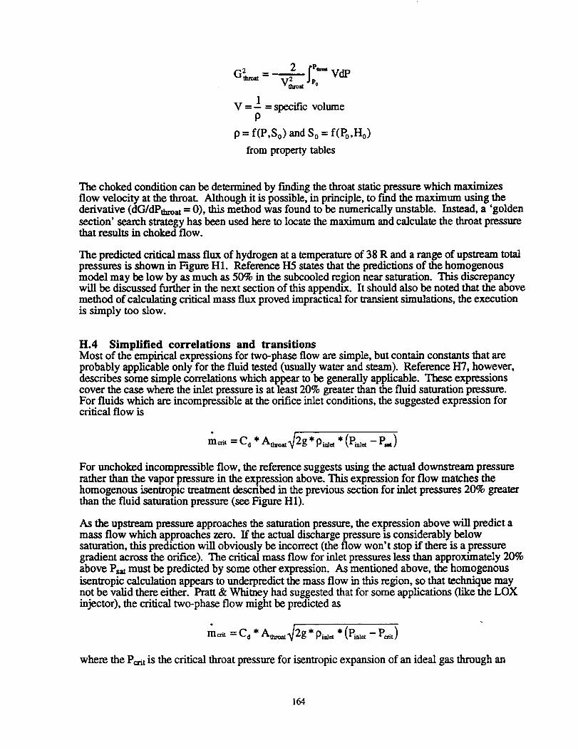
V = _I= specificvolume

P

p = f(P,So)and SO= f(Po,Ho)

from property tables

The choked condition can be determined by finding the throat static pressure which maximizesflow velocity at the throat. Although it is possible, in principle, to find the maximum using thederivative (dG/dPthroat = 0), this method was found to be numerically unstable. Instead, a 'golden

section' search strategy has been used here to locate the maximum and calculate the throat pressurethat results in choked flow.

The predicted critical mass flux of hydrogen at a temperature of 38 R and a range of upstream totalpressures is shown in Figure HI. Reference H5 states that the predictions of the homogenousmodel may be low by as much as 50% in the subcooled region near saturation. This discrepancywill be discussed further in the next section of this appendix. It should also be noted that the abovemethod of calculating critical mass flux proved impractical for transient simulations, the executionis simply too slow.

H.4 Simpfified correlations and transitionsMost of the empirical expressions for two-phase flow are simple, but contain constants that areprobably applicable only for the fluid tested (usually water and steam). Reference I-I7, however,describes some simple correlations which appear to be generally applicable. These expressionscover the case where the inlet pressure is at least 20% greater than the fluid saturation pressure.For fluids which axe incompressible at the orifice inlet conditions, the suggested expression forcritical flow is

m_it = Cd * A_o_t42g * pi_t * (Pt,1, - Pro)

For unchoked incompressible flow, the reference suggests using the actual downslream pressurerather than the vapor pressure in the expression above. This expression for flow matches thehomogenous isentropic treatment described in the previous section for inlet pressures 20% greaterthan the fluid saturation pressure (see Figure HI).

As the upstream pressure approaches the saturation pressure, the expression above will predict amass flow which approaches zero. If the actual discharge pressure is considerably belowsaturation, this prediction will obviously be incorrect (the flow won't stop if there is a pressuregradient across the orifice). The critical mass flow for inlet pressures less than approximately 20%

above Psat must be predicted by some other expression. As mentioned above, the homogenous

isentropic calculation appears to underpredict the mass flow in this region, so that technique maynot be valid there either. Pratt & Whimey had suggested that for some applications (like the LOXinjector), the critical two-phase flow might be predicted as

o

m_, = Cd * A_,_ 42g* p,_ * (P_o_ - P_, )

where the Pea-it is the critical throat pressure for isentropic expansion of an ideal gas through an

164

orifice. In fact, Pratt& Whitneyhassuggestedthatthespecificheatratiousedto calculatethispressurebe 1.4(evenfor LOX). Consequently,Petitis the inlet totalpressuredividedby 1.89.This assumption may be associated with the manner in which Pratt & Whitney determined theeffective areas of the cooldown valves and LOX injector from the calibration test data.

Why should there be different expressions for critical two-phase flow in different components?After some consideration, we arrived at the following explanation. For sufficiently high inlet

pressures and sufficiently low discharge pressures, the fluid will flash to vapor at the throat (butnot upstream of it). Under these conditions, the flow characteristics would still be that of anincompressible fluid, but the flashing would create an area near the throat that would be equal tothe saturation pressure of the fluid, even if the downstream pressure continued to decline (seeFigure H2). As the inlet pressure decreases, there will be a threshold where the static pressure ofthe fluid at the throat will drop below the saturation pressure. At this point, the fluid will flash

upstream of the throat. If we assume that the flashing creates densities low enough and fluidvelocities high enough to go sonic at the throat, then the throat pressure will be limited by thecorresponding critical pressure. Often cryogens (including hydrogen and oxygen) behave muchlike an ideal gas for pressures only slightly below the point of vaporization. This tends to supportusing the critical pressure as defined for flow of an ideal gas through the orifice. The flow stillproceeds primarily as an incompressible fluid, but it becomes gaseous near the throat and itschoking is governed by gas laws. For sufficiently low inlet pressures, the flow will be entirelyvapor. These arguments have lead to the following expressions and rules for the new systemmodel, as were also cited in the main report.

m = C d *A* a]2g * P,,,,t * 5p

5p = (Pinlet -Pexit) for Pexit > Psat

_p = (Pinlet -Pexit) for Petit < Psat and Pexit > Pcrit

_p = (Pinlet - Psat) for Petit > Psat and Pexit < Psat

_p = (Pinlet - Petit) for Petit < Psat and Pexit < Petit

where Psat = function of Sinlet looked up from tables

¥

,,,d p,,,,=(t,'y+l)

The predicted flow rate using this method is shown in Figure HI, compared with the homogenousflux predictions. There was insufficient data in the literature to make a comparison with theheterogenous model described in Reference H4. The simple hybrid correlation described abovepredicts a flux of approximately twice that of the integral method near saturation. As was notedpreviously, Reference H5 suggests that this would better match experimental data and predictions

of a heterogenous model.

This simple model provides a robust, efficient, and stable solution for two-phase choked andunchoked flows in the RL10 system during start and shutdown. This model also appears tocorrelate well with the available RL10 engine test data for the fuel cooldown valves and LOX

injector.

165

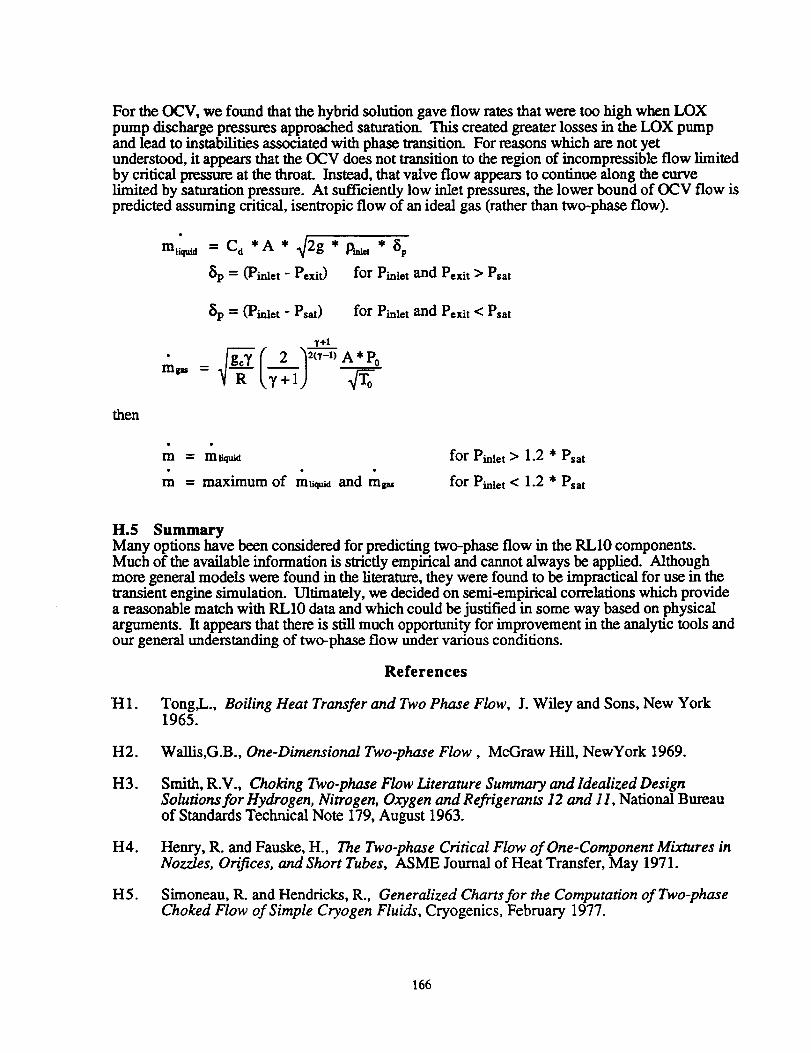
For the OCV, we found thatthe hybridsolutiongave flow ratesthatwere too high when LOX

pump dischargepressuresapproached saturation.This createdgreaterlossesinthe LOX pump

and leadto instabilitiesassociatedwith phase transition.For reasonswhich are not yet

understood,itappearsthatthe OCV does not transitiontotheregionof incompressibleflow limited

by criticalpressureatthe throat.Instead,thatvalveflow appearsto continuealong thecurvelimitedby saturationpressure.At sufficientlylow inletpressures,the lower bound of OCV flow is

predictedassuming critical,isentropicflow of an idealgas (ratherthan two-phase flow).

mliq_id "- C d * A * 3/2g * p_ * _p

_p = (Pinlet - Pexit) for Pinlet and Pexit > Psat

_p -- (Pinlet - Psat) for Pinlet and Pexit < Psat

¥+1

tv+l)

then

m = m fiquid

m = maximum of muq._d and rag.

for Pinlet > 1.2 * Psat

for Pinlet < 1.2 * Psat

H.5 SummaryMany options have been considered for predicting two-phase flow in the RL10 components.Much of the available information is strictly empirical and cannot always be applied. Althoughmore generalmodels were found intheliterature,theywere found tobe impracticalforuse inthe

transientenginesimulation.Ultimately,we decidedon semi-empiricalcorrelationswhich provide

a reasonablematch with RLIO dataand which could be justifiedinsome way based on physical

arguments. Itappearsthatthereisstillmuch opportunityforimprovement intheanalytictoolsand

our generalunderstandingoftwo-phase flow under variousconditions.

References

H1. Tong,L,., Boiling Heat Transfer and Two Phase Flow, J. Wiley and Sons, New York1965.

H2. Wallis,G.B., One-Dimensional Two-phase Flow, McGraw Hill, NewYork 1969.

H3. Smith, R.V., Choking Two-phase Flow Literature Summary and Idealized DesignSolutions for Hydrogen, Nitrogen, Oxygen and Refrigerants 12 and 11, National Bureauof Standards Technical Note 179, August 1963.

H4. Henry, R. and Fauske, H., The Two-phase Critical Flow of One-Component Mixtures inNozzles, Orifices, and Short Tubes, ASME Journal of Heat Transfer, May 1971.

H5. Simoneau, R. and Hendricks, R., Generalized Charts for the Computation of Two-phaseChoked Flow of Simple Cryogen Fluids, Cryogenics, February 1977.

166

H6.

H7.

Hendricks, R. and Stetz, T., Flow Rate and Pressure Profiles for One to Four Axially

Alined Orifice Inlets, NASA TP-2460, May 1985.

Applied Physics Laboratory, JANNAF Rocket Engine Performance Test Data Acquisitionand Interpretation Manual, CPIA Publication 245, April 1975.

167

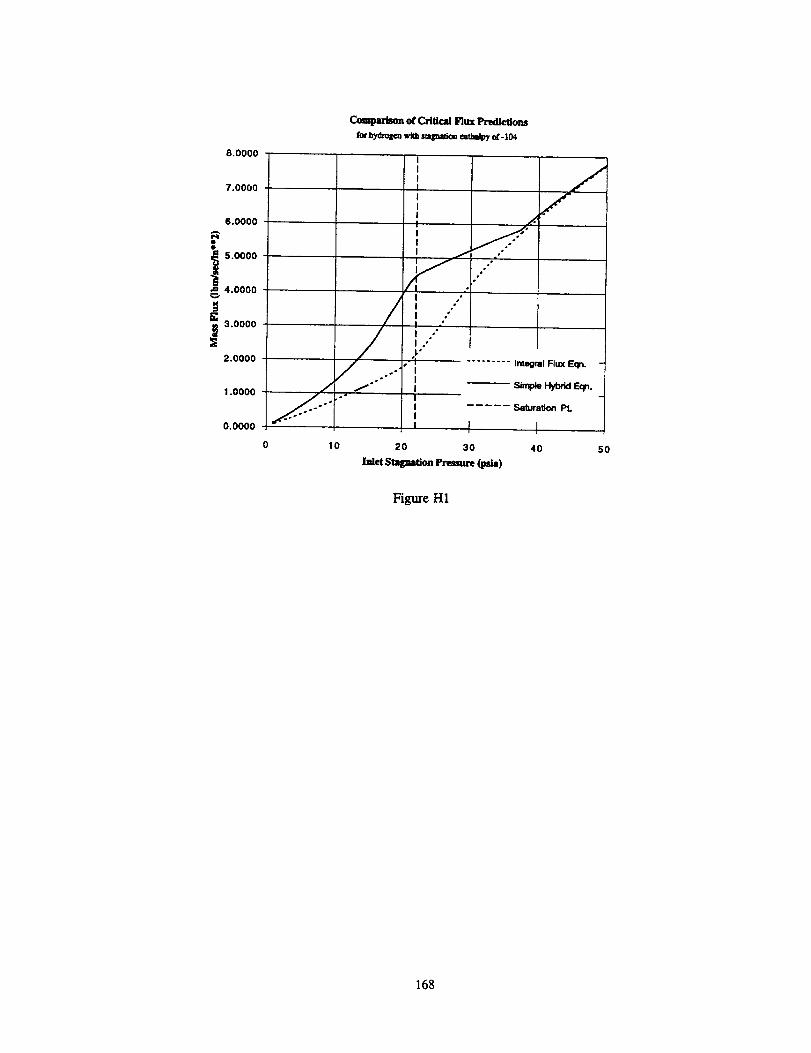
8.0000

7.0000

6.0000

i 5.00004.0000

3.0000

2.0000

1.0000

0.0000

/

Compm4son of CrlUca] Flux PrecUceons

f_ withm_ _,u_t_ _-104

IIII

0 10 20

IIIII

I .t

I °i °n

I t °

Ia °I..

V

#- e_I

!!

......... Integral Flux Eqn.

..... Satura_on pt

I i

30 40

Inlet Stagnation Pressure (psJa)

5O

Figure HI

168

Simple Incompressible Correlations forCritical Two-Phase Flow through an Orifice

L utturated /'--'-

vapor

Psat_ fO

2

Case 1: fluid flashes at the throat (but not upstream of it).

[ flOW--" Cd*Athremt* (2g * Pl* (Pl-'Psat_)lf_ ]

P2

Case 2: fluid flashes upstream of throat

] fl°w ffi Cd'Athr°at" (2g * PI* (PI" Petit))1/2 ]

where P_t is based on ideal gas assumptions

Figure H2

169

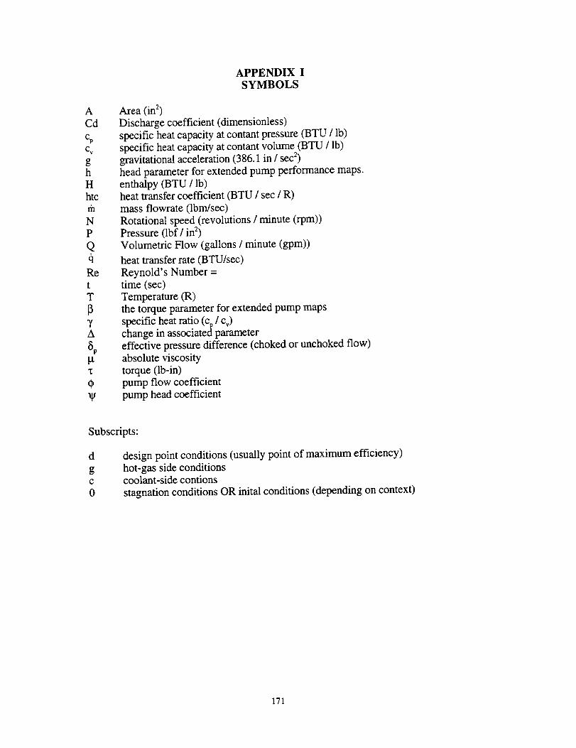
A

Cd

%Cv

gh

H

htcrfi

N

P

Q

Re

t

T

A

5pg

0

APPENDIX I

SYMBOLS

Area (in z)

Discharge coefficient (dimensionless)

specific heat capacity at contant pressure (BTU / lb)

specific heat capacity at contant volume (BTU / lb)

gravitational acceleration (386.1 in / sec 2)

head parameter for extended pump performance maps.

enthalpy (BTU / lb)heat transfer coefficient (BTU / sec / R)

mass flowrate (lbm/sec)

Rotational speed (revolutions / minute (rpm))

Pressure (lbf / in 2)

Volumetric Flow (gallons / minute (gpm))

heat transfer rate (BTU/sec)

Reynold's Number =time (sec)

Temperature (R)

the torque parameter for extended pump maps

specific heat ratio (% / cV)change in associated parameter

effective pressure difference (choked or unchoked flow)

absolute viscosity

torque (lb-in)

pump flow coefficient

pump head coefficient

Subscripts:

d

gC

0

design point conditions (usually point of maximum efficiency)

hot-gas side conditionscoolant-side contions

stagnation conditions OR inital conditions (depending on context)

171

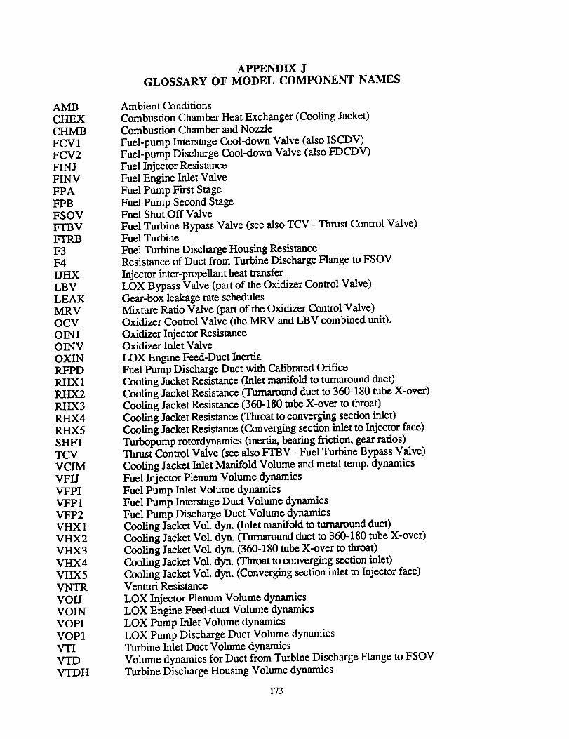
AMB

CHEX

CHMBFCV1

FCV2

FINJ

FINV

FPA

FPB

FSOVFTBV

FTRB

F3F4

IJI-IX

LBVLEAK

MRV

OCV

OINJ

OINVOXIN

RFPD

RHX1RHX2

RHX3

RHX4

RHX5

SHFT

TCV

VCIM

VFIJ

VFPI

VFP1

VFP2VHX1

VHX2

VHX3

VHX4

VHX5

VNTR

VOIJ

VOIN

VOPI

VOP1

VTI

VTD

VTDH

APPENDIX J

GLOSSARY OF MODEL COMPONENT NAMES

Ambient Conditions

Combustion Chamber Heat Exchanger (Cooling Jacket)

Combustion Chamber and Nozzle

Fuel-pump Interstage Cool-down Valve (also ISCDV)

Fuel-pump Discharge Cool-down Valve (also FDCDV)

Fuel Injector Resistance

Fuel Engine Inlet Valve

Fuel Pump First Stage

Fuel Pump Second StageFuel Shut Off Valve

Fuel Turbine Bypass Valve (see also TCV - Thrust Control Valve)Fuel Turbine

Fuel Turbine Discharge Housing ResistanceResistance of Duct from Turbine Discharge Flange to FSOV

Injector inter-propeUant heat transferLOX Bypass Valve (part of the Oxidizer Control Valve)

Gear-box leakage rate schedules

Mixture Ratio Valve (part of the Oxidizer Control Valve)Oxidizer Control Valve (the MRV and LBV combined unit).

Oxidizer Injector ResistanceOxidizer Inlet Valve

LOX Engine Feed-Duct Inertia

Fuel Pump Discharge Duct with Calibrated OrificeCooling Jacket Resistance (Inlet manifold to turnaround duct)

Cooling Jacket Resistance (Turnaround duct to 360-180 tube X-over)

Cooling Jacket Resistance (360-180 tube X-over to throat)

Cooling Jacket Resistance (Throat to converging section inlet)

Cooling Jacket Resistance (Converging section inlet to Injector face)

Turbopump rotordynamics (inertia, bearing friction, gear ratios)Thrust Control Valve (see also FTBV - Fuel Turbine Bypass Valve)

Cooling Jacket Inlet Manifold Volume and metal temp. dynamics

Fuel Injector Plenum Volume dynamics

Fuel Pump Inlet Volume dynamics

Fuel Pump Interstage Duct Volume dynamics

Fuel Pump Discharge Duct Volume dynamics

Cooling Jacket Vol. dyn. (Inlet manifold to turnaround duct)Cooling Jacket Vol. dyn. (Turnaround duct to 360-180 tube X-over)

Cooling Jacket Vol. dyn. (360-180 tube X-over to throat)

Cooling Jacket Vol. dyn. (Throat to converging section inlet)

Cooling Jacket Vol. dyn. (Converging section inlet to Injector face)Venturi Resistance

LOX Injector Plenum Volume dynamics

LOX Engine Feed-duct Volume dynamics

LOX Pump Inlet Volume dynamics

LOX Pump Discharge Duct Volume dynamicsTurbine Inlet Duct Volume dynamics

Volume dynamics for Duct from Turbine Discharge Flange to FSOV

Turbine Discharge Housing Volume dynamics

173

.

.

.

.

.

.

.

.

.

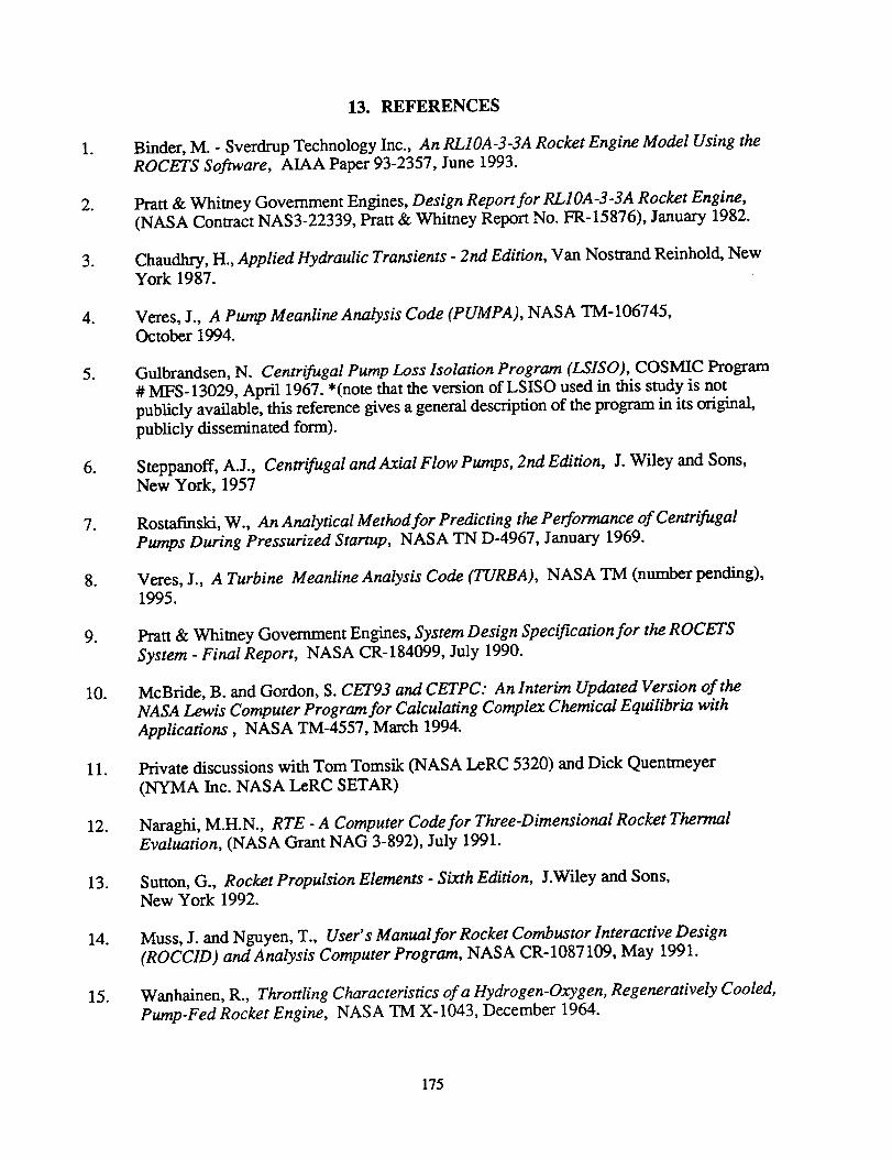
10.

11.

12.

13.

14.

15.

13. REFERENCES

Binder, M. - Sverdrup Technology Inc., An RLIOA-3-3A Rocket Engine Model Using the

ROCETS Software, AIAA Paper 93-2357, June 1993.

Pratt & Whitney Government Engines, Design Report for RLI OA-3-3A Rocket Engine,

(NASA Contract NAS3-22339, Pratt & Whitney Report No. FR-15876), January 1982.

Chaudhry, H., Applied Hydraulic Transients - 2nd Edition, Van Nostrand Reinhold, New

York 1987.

Veres, J., A Pump Meanline Analysis Code (PUMPA), NASA TM-106745,

October 1994.

Gulbrandsen, N. Centrifugal Pump Loss Isolation Program (LSISO), COSMIC Program

# MFS- 13029, April 1967. *(note that the version of LSISO used in this study is not

publicly available, this reference gives a general description of the program in its original,

publicly disseminated form).

Steppanoff, A.J., Centrifugal and Axial Flow Pumps, 2nd Edition, J. Wiley and Sons,

New York, 1957

Rostafmski, W., An Analytical Method for Predicting the Performance of Centrifugal

Pumps During Pressurized Startup, NASA TN D-4967, January 1969.

Veres, J., A Turbine MeanIine Analysis Code (TURBA), NASA TM (number pending),

1995.

Pratt & Whitney Government Engines, System Design Specification for the ROCETS

System - Final Report, NASA CR-184099, July 1990.

McBride, B. and Gordon, S. CET93 and CETPC: An Interim Updated Version of the

NASA Lewis Computer Program for Calculating Complex Chemical Equilibria with

Applications, NASA TM-4557, March 1994.

Private discussions with Tom Tomsik (NASA LeRC 5320) and Dick Quentmeyer

(NYMA Inc. NASA LeRC SETAR)

Naraghi, M.H.N., RTE - A Computer Code for Three-Dimensional Rocket ThermalEvaluation, (NASA Grant NAG 3-892), July 1991.

Sutton, G., Rocket Propulsion Elements - Sixth Edition, J.Wiley and Sons,

New York 1992.

Muss, J. and Nguyen, T., User's Manual for Rocket Combustor Interactive Design

(ROCCID) and Analysis Computer Program, NASA CR-1087109, May 1991.

Wanhainen, R., Throttling Characteristics of a Hydrogen-Oxygen, Regeneratively Cooled,

Pump-Fed Rocket Engine, NASA TM X-1043, December 1964.

175

16.

17.

18.

19.

20.

23.

24.

25.

26.

27.

28.

Nickerson,G., Two-Dimensional Kinetics (TDK) Nozzle Performance ComputerProgram - Users Manual, (NASA Contract NAS8-39048), March 1993.

Crane Company, Technical Paper No. 410, Flow of Fluids Through Valves, Fittings, andPipe, 1982.

Crane Co. and ABZ Inc., Crane Companion to Flow of Fluids Through Valves, Fittings,

andPipe, (software), 1992.

Henry, R. and Fauske, H., The Two-phase Critical Flow of One-Component Mixtures in

Nozzles, Orifices, and Short Tubes, ASME Journal of Heat Transfer, May 1971.

Tong, L., Boiling Heat Transfer and Two Phase Flow, J. Wiley and Sons, New York1965.

Wallis, G.B., One-Dimensional Two-phase Flow, McGraw Hill, NewYork 1969.

Simoneau, R. and Hendricks, R., Generalized Charts for the Computation of Two-phase

Choked Flow of Simple Cryogen Fluids, Cryogenics, February 1977.

Applied Physics Laboratory, JANNAF Rocket Engine Performance Test Data Acquisition

and Interpretation Manual, CPIA Publication 245, April 1975.

Smith, R.V., Choking Two-phase Flow Literature Summary and Idealized Design

Solutions for Hydrogen, Nitrogen, Oxygen and Refrigerants 12 and 11, National Bureau

of Standards Technical Note 179, August 1963.

Streeter, V. and Wylie, E., Fluid Mechanics - Seventh Edition, McGraw Hill,New York 1979.

Perry, R. and Chilton, C., Chemical Engineer's Handbook - Fifth Edition, McCrraw Hill,New York 1973.

Private discussions with Todd Denman, Pratt & Whimey Government Engines, WestPalm Beach, Florida

RL- 10 Start Capability Working Group (govemment/'mdustry cooperative), AC-71 Failure

Investigation - Final Report, (no contract or report number given), December 1993.

176

Form Approved

REPORT DOCUMENTATION PAGE OMB No. 0704-0188

Pub,icreportingburdenforthisco,lecliono1in,ormatlonis estimatedto average1.hourper:n_or_ninC_:_ndgc_emantsf_V_enWgntghiir_btu_tn:_;_SmatearCe_o;_r-----_pe_t_t_sgatheringandmaintainingthe dataneeded,andcorr.l_etmgano.revlewmgme=c_=,.,_-_u,,,u,_,u,..... '_enlicesOirectorate'f_rnformationOperationsand Repoas,1215JeffersonincludinSU tionslot reouclngmlsouroen,lu w¢_.._¢_, _,_=_,_........ ...........collectionof information. .. g. g=.g_...... = .- .,.^ _;_ ._ u=.=_=m,mtandBudaetPaoetworkReductionProjec_(0704-0188).wasnmgton,uL. L_.rj.DavisHighway.S,_,it_1204.Ar,nglon.vA _zzu,:-_Ju<:,..,u _vt.o _ .......... .-_,-.,.- = ,

1. AGENCY USE ONLY (Leave blank) 2. REPORT DATE 3. REPORT TYPE AND DATES COVERED

January 1997 Technical Memorandum

4. TITLE AND SUBTITLE

RL10A-3-3A Rocket Engine Modeling Project

6. AUTHOR(S)

Michael Binder, Thomas Tomsik, and Joseph P. Veres

7. PERFORMING ORGANIZATION NAME(S) AND ADDRESS(ES)

National Aeronautics and Space AdministrationLewis Research CenterCleveland, Ohio 44135-3191

9. SPONSORING/MONITORING AGENCY NAME(S) AND ADDRESS(ES)

National Aeronautics and Space Administration

Washington, D.C. 20546-0001

5. FUNDING NUMBERS

WU-564--09-10

8. PERFORMING ORGANIZATIONREPORT NUMBER

E-10414

10. SPONSORING/MONi/uRINGAGENCY REPORT NUMBER

NASA TM- 107318

11. SUPPLEMIEICFARY NOTES

Michael Binder, NYMA, Inc., 2001 Aerospace Parkway, Brook Park, Ohio 44142 (work funded under NASA ContractNAS3-27186); Thomas Tomsik and Joseph P. Veres, NASA Lewis Research Center. Responsible person, Thomas Tomsik

u_ganization code 5340, (216) 977-7519.12a. DISTRIBUTION/AVAILABILITY STATEMENT 12b. DI_FUBUTION CODE

Unclassified -Unlimited

Subject Category 20

This publication is awilahle from the NASA Center for AeroSpace Information, (301) 621--0390

13. ABSTRACT (Maximum 200 words)

Two RL10A-3-3A rocket engines comprise the main propulsion system for the Centaur upper stage vehicle. Centaur is used with both

Titan and Arias latmch vehicles, carrying military and civilian payloads from high altitudes into orbit and beyond. The RL10 has

delivered highly reliable service for the past 30 years. Recently, however, there have been two in-flight failures which have refocused

attention on the RL10. This heightened interest has sparked a desire for an independent RL10 modeling capability within NASA and the

Air Force. Pratt & Whimey, which presently has the most detailed model of the RL10, also sees merit in having an independent model

which could be used as a cross-check with their own simulations. The Space Propulsion Technology Division (SPTD) at the NASA

Lewis Research Center has developed a computer model of the RL10A-3-3A. A project team was formed, consisting of experts in the

areas of turbomachinery, combustion, and heat transfer. The overall goal of the project was to provide a model of the entire RL10 rockel

engine for government use. In the course of the project, the major engine components have been modeled using a combination of simpl_correlations and detailed component analysis tools (computer codes). The results of these component analyses were veritied with data

provided by Pratt & Whimey. Select modeling results and test data curves were then integrated to form the RL10 engine system model.

The purpose of this report is to introduce the reader to the RL10 rocket engine and to describe the engine system model. The RL10engine and its application to U.S. launch vehicles are described first, followed by a summary of the SPTD project organization, goals,

and accomplishments. Simulated output from the system model are shown in comparison with test and flight data for start transient,

steady state, and shut-down transient operations. Detailed descriptions of all component analyses, including those not sdected for

integration with the system model, are included as appendices.

SECURFrY CLASSIFICATIONOF REPORT

Uncl_z_-_ified

14. SUBJECT TERMS

RL10; RL10A-3-3A; Rocket engine; Simulation; Models

17. 18. SECURITY CLASSIFICATIONOF THIS PAGE

Unclassified

NSN 7540-01-280-5500

19. SECURITY CLASSIFICATIONOF ABSTRACT

Unclassified

•15. NU._U_REROF PAGES

18216. PRICE CODE

A0920. LIMITATION OF AB._TRACT

Standard Form 298 (Rev. 2-89)PrescnToedby ANSI Std. Z39-18298-102