RIVER STAGE FORECASTING USING

WAVELET TECHNIQUE

By-

1. Rajeev Ranajan Sahay, Assistant Professor,

Department of Civil Engineering,

BIT, Mesra.

2. Vinit Sehgal, BE

Department of Civil Engineering,

BIT, Mesra.

FLOOD PRONE RIVER KOSI

River Kosi,a tributary of Ganga River, is often

called the ‘Sorrow of Bihar ‘ because of the

widespread destruction caused by the river

due to frequent floods in it.

About 90% of the catchment area of River

Kosi is flood prone.During floods,water stage

of Kosi increases to about 18 times its

average value.

Floods generally cause great devastation due to their poor and late estimation. A recent flood occurred in River Kosi in Monsoon season of 2008 that lead to heavy loss of man and material.

In event of occurring of a flood, authorities and people of the area are not forewarned of the incoming high flood, thereby, not allowing them enough time for taking up appropriate flood-fighting measures.

BASIN MAP OF KOSI RIVER (NORTH BIHAR)

RIVER STAGE FORECASTING

To predict river stage accurately and timely, several mathematical models are employed.

These are based on several techniques. Some of them include:

Auto Regression(AR)

Artificial Neural Networks(ANN)

Genetic Algorithm(GA)

Genetic Programming (GP)

Discrete Wavelet Transform(DWT) etc.

DATA ANALYSIS

For Flood forecasting, 231 monsoon stage data of year 2005 and 2006 is used as derivation set data.

120 stage data of year 2007 is used as verification set data for verifying the ANN and DWT models.

The developed models are applied to forecast one-day ahead flood levels of Kosi River.

PARAMETERS OF STAGE DATA

The statistical parameters of stage data is

given in the given Table.

Parameter Verification data

(m)

Derivation data

(m)

Min. Stage 73.70 72.88

Max. stage 74.95 74.98

Mean stage 74.39 74.22

Std. Dev. 0.24 0.31

Range 1.25 2.10

WAVELET REGRESSION MODEL

Wavelet Regression Model is a recent technique to model complex and nonlinear hydrological processes without underlying physics being explicitly provided.

Wavelet models have a strong generalization ability, which means that once mother wavelet is properly selected, they are able to provide accurate results even for cases they have never seen before.

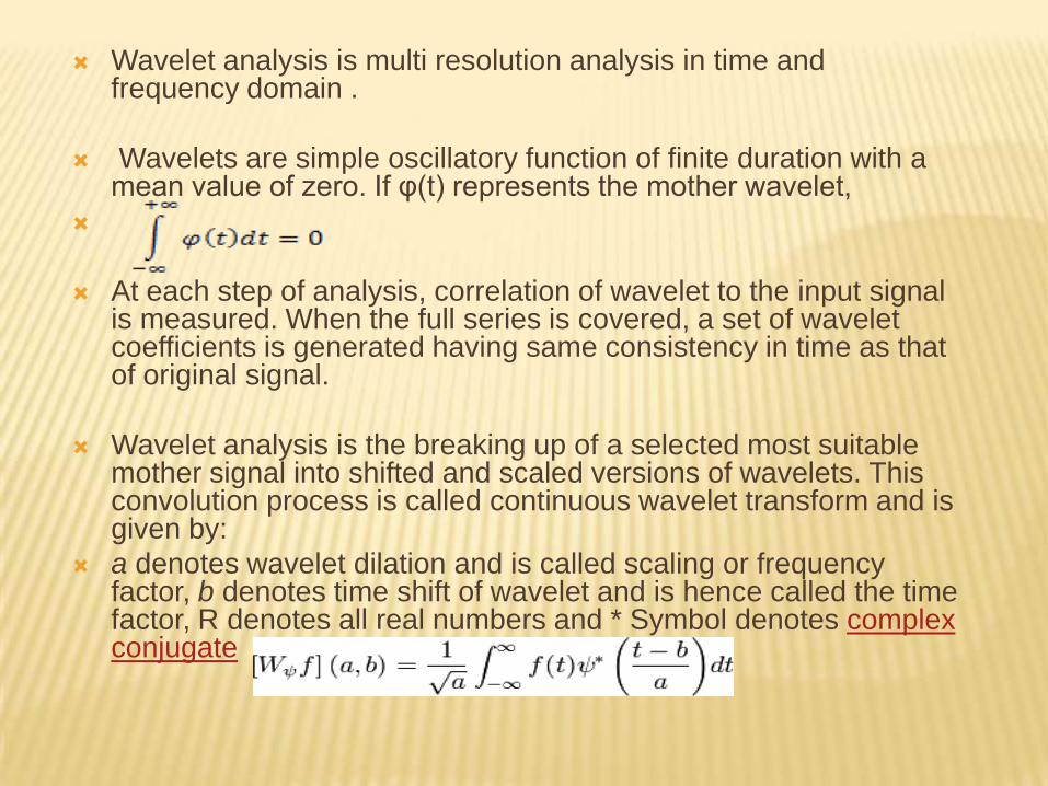
Wavelet analysis is multi resolution analysis in time and frequency domain .

Wavelets are simple oscillatory function of finite duration with a mean value of zero. If φ(t) represents the mother wavelet,

At each step of analysis, correlation of wavelet to the input signal is measured. When the full series is covered, a set of wavelet coefficients is generated having same consistency in time as that of original signal.

Wavelet analysis is the breaking up of a selected most suitable mother signal into shifted and scaled versions of wavelets. This convolution process is called continuous wavelet transform and is given by:

a denotes wavelet dilation and is called scaling or frequency factor, b denotes time shift of wavelet and is hence called the time factor, R denotes all real numbers and * Symbol denotes complex conjugate

Figure showing scaled and translated wavelet on a given signal.

•

Since most of the natural time series are

discreet in nature, Discrete Wavelet

Transform is to applied for decomposition

and reconstruction of time series.

DWT FILTERS

DWT operates as set of two functions or

filters i.e. high pass filter and low pass filter.

The original time series is decomposed

through a process consisting of a number of

successive filtering steps giving

a) Approximation(Low frequency terms)

b) Details(High frequency terms)

Flow Chart for Decomposition of Time Series Wave

MATLAB DECOMPOSITION OF TIME SERIES

DWT PROCESS

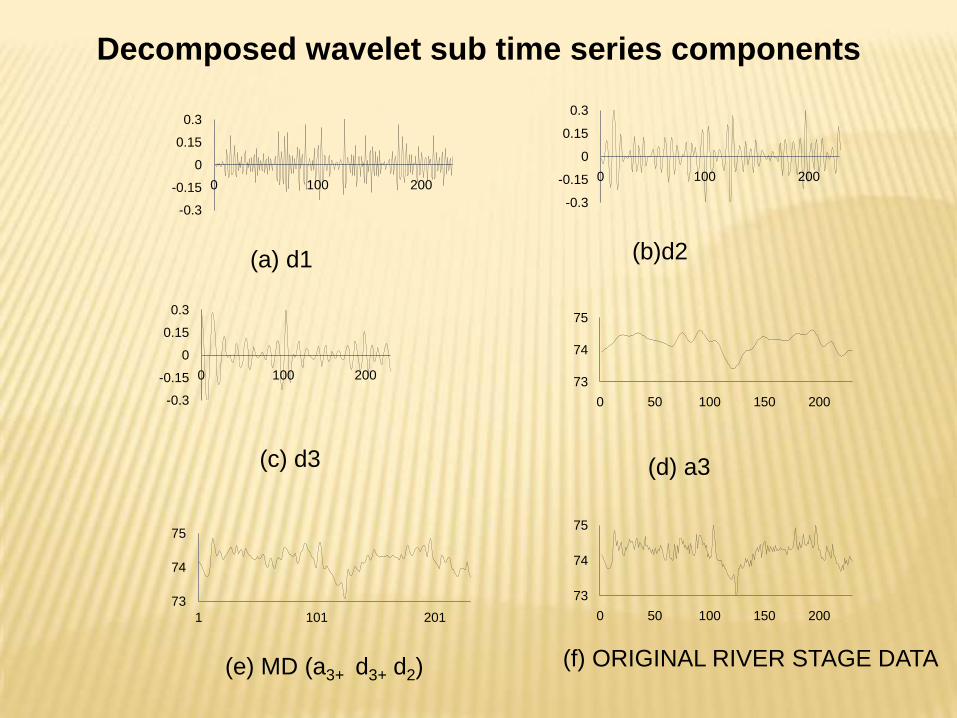
The derivation set data was decomposed uptothree levels of decomposition to obtain d1,d2,d3,a3 (i.e. the details and the approximation).

d1,d2,d3,a3 were arranged in various lags and their correlation with the original derivation set data was obtained.

TABULATION OF CORRELATION

coif5 Average value of R

d10.053

d20.144

d30.155

a30.79

Average correlation for d1 is

lowest . This indicates that it

may induce irregularity in

the mathematical model.

Hence, it is eliminated from

further analysis.

FORMATION OF WR MODELS

d1 component was neglected and the d2, d3

and a3 so obtained, were fed to three AR models separately as independent inputs. The outputs of these AR models were added to obtain the predicted river stage Sp. This provided wavelet regression model 1 (WR1 model).

Another wavelet regression model had slightly different methodology. A modified series, obtained by adding d2, d3 and a3 (MD) was used as input to Auto regression model. This provided Wavelet regression model 2 (WR2 model).

-0.3

-0.15

0

0.15

0.3

0 100 200

-0.3

-0.15

0

0.15

0.3

0 100 200

-0.3

-0.15

0

0.15

0.3

0 100 20073

74

75

0 50 100 150 200

73

74

75

1 101 201

73

74

75

0 50 100 150 200

(f) ORIGINAL RIVER STAGE DATA(e) MD (a3+ d3+ d2)

(d) a3(c) d3

(b)d2(a) d1

Decomposed wavelet sub time series components

STRUCTURE OF WR1 AND WR2 MODEL

RESULTS FOR WR MODELS

DERIVATION PERIOD VARIFICATION PERIOD

WR1 CC RMSE (m) CC RMSE (m)

MD t-1 0.925 0.129 0.912 0.104

MD t-1, MD t-2 0.959 0.096 0.945 0.082

MD t-1, MD t-2, MD t-3 0.959 0.096 0.947 0.0817

MD t-1, MD t-2, MD t-3, MD t-4 0.963 0.091 0.951 0.079

MD t-1, MD t-2, MD t-3, MD t-4, MDt-5 0.963 0.091 0.951 0.079

WR2 CC RMSE (m) CC RMSE (m)

MD t-1 0.893 0.140 0.901 0.110

MD t-1, MD t-2 0.917 0.124 0.914 0.104

MD t-1, MD t-2, MD t-3 0.939 0.107 0.932 0.092

MD t-1, MD t-2, MD t-3, MD t-4 0.943 0.104 0.938 0.089

MD t-1, MD t-2, MD t-3, MD t-4, MDt-5 0.945 0.103 0.943 0.085

The model for river stage for Kosi River using the best performing WR1model is given as:

St = 0.707+(1.319 MDd2(t-1)-1.99 MDd2(t-2) +1.30 MDd2(t-3)

-0.95 MDd2(t-4) +0.193 MDd2(t-5) )+(2.83 MDd3(t-1)-3.47 MDd3(t-2)

+1.93 MDd3(t-3)-0.27 MDd3(t-4)-0.164 MDd3(t-5) )+(3.87 MDa3(t-1)

-5.95 MDa3(t-2)+4.437 MDa3(t-3)-1.54 MDa3(t-4)+0.179 MDa3(t-5)

Similarly for WR2 model, the equation describing river stage with best results is given by:

St = 2.36+ 2.26 MDt-1 - 2.67 MDt-2 + 2.15 MDt-3 -1.12 MDt-4 + 0.34 MDt-5

EFFECT OF INCREASING THE NUMBER OF LAGS

In the models for river stage of Kosi River, the river stage

values only up to last five days are involved. The models

involving higher number of previous stage data were also

tested but it was observed that there was no significant

increase in the result of the models in terms of coefficient of

correlation.

0.87

0.88

0.89

0.9

0.91

0.92

0.93

0.94

0.95

0.96

1 2 3 4 5 6 7 8 9 10

R v

alu

e

No. of previous day's data involved

EFFECT OF USING DIFFERENT WAVELETS

0.820.840.860.88

0.90.920.940.96

haar db3 db5 db10 sym9 coif5 bior6.8 rbio6.8 dmey

R v

alu

e

Wavelet used in model formation

0

0.02

0.04

0.06

0.08

0.1

0.12

0.14

haar db3 db5 db10 sym9 coif5 bior6.8 rbio6.8 dmey

RM

SE

Wavelet used in model formation

ANN PROCEDURE

As in the case of the WR models, five input combinations based on previous Daily River stages were used as inputs to the ANN models to estimate the current stage value.

The output node consisted of stage S t for the current day.

The three input nodes in this network represent the stages at days t - 1, t - 2, and t – 3 (S t-1, S t-2, and S

t-3), and the unique output represents the stage (St) to be predicted.

RMSE & R STATISTICS OF ANN

MODEL

Model Inputs

ANN

STRUCTURE

DERIVATION

PERIOD

VARIFICATION

PERIOD

CC RMSE (m) CC RMSE (m)

S t-1 (1,4,1) 0.8150.179

0.7870.152

S t-1, S t-2 (2,6,1) 0.8190.297

0.8210.147

S t-1, S t-2, S t-3 (3,8,1) 0.8190.180

0.8270.146

S t-1, S t-2, S t-3, S t-4 (4,8,1) 0.8220.179

0.8290.146

S t-1, S t-2, S t-3, S t-4, St-5 (5,10,1)0.823 0.179 0.831 0.146

COMPARISON OF PERFORMANCE

Performance indices considered for comparing results from

different models are the root mean square error (RMSE),

coefficient of correlation (CC) and the discrepancy

ratio.(DR).RMSE, CC, DR are defined as:

ACCURACY OF MODEL

If the accuracy of the model can be defined as

percentage of DR values falling between -0.001 to

0.001i.e. Predicted values of river stage lying

between 99.8% and 100.2% of the measured

values.

COMPARISON OF PERFORMANCE

Name of the

modelRMSE (m) CC DR Range Accuracy in %

WR 1 0.079 0.95 -0.0016 to 0.0012 97.41

WR 2 0.085 0.94 -0.0014 to 0.0015 95.65

ANN 0.153 0.83 -0.002 to 0.0027 81.74

0

5

10

15

20

25

30

35

40

45

ANN WR2

WR1

COMPARISON OF DISCREPANCY RATIO FOR VARIOUS MODELS.

COMPARISON OF RESULT OF DIFFERENT MODELS

73.70

73.90

74.10

74.30

74.50

74.70

74.90

1 4 7

10

13

16

19

22

25

28

31

34

37

40

43

46

49

52

55

58

61

64

67

70

73

76

79

82

85

88

91

94

97

100

103

106

109

112

115

Riv

er

Sta

ge

(m

)

No. of days in verification period

Original River stage Stage predicted using ANN model

73.70

73.90

74.10

74.30

74.50

74.70

74.90

1 4 7

10

13

16

19

22

25

28

31

34

37

40

43

46

49

52

55

58

61

64

67

70

73

76

79

82

85

88

91

94

97

100

103

106

109

112

115

Riv

er

Sta

ge

(m

)

No. of days in Verification period

Original River stage Stage predicted using WR1 model

73.70

73.90

74.10

74.30

74.50

74.70

74.90

1 4 7

10

13

16

19

22

25

28

31

34

37

40

43

46

49

52

55

58

61

64

67

70

73

76

79

82

85

88

91

94

97

100

103

106

109

112

115

Riv

er

Sta

ge (

m)

No. of daya in verification period

Original River stage Stage predicted using WR2 model

73.70

73.90

74.10

74.30

74.50

74.70

74.90

1 4 7

10

13

16

19

22

25

28

31

34

37

40

43

46

49

52

55

58

61

64

67

70

73

76

79

82

85

88

91

94

97

100

103

106

109

112

115

Riv

er

Sta

ge

(m

)

Original River stage Stage predicted using ANN model

73.70

73.90

74.10

74.30

74.50

74.70

74.90

1 4 7

10

13

16

19

22

25

28

31

34

37

40

43

46

49

52

55

58

61

64

67

70

73

76

79

82

85

88

91

94

97

100

103

106

109

112

115

Riv

er

Sta

ge

(m

)

Original River stage Stage predicted using WR1 model

73.70

73.90

74.10

74.30

74.50

74.70

74.90

1 4 7

10

13

16

19

22

25

28

31

34

37

40

43

46

49

52

55

58

61

64

67

70

73

76

79

82

85

88

91

94

97

100

103

106

109

112

115

Riv

er

Sta

ge (

m)

Original River stage Stage predicted using WR2 model

CONCLUSION

The WR model has been found to perform better than ANN models.

WR model has high value of R, low RMSE and greater accuracy as compared to ANN.

It was also observed that more number of previous days’ stage data did not give much increment to the performance of any model. Hence models involving only up to five previous days’ stage data were studied.

THANK YOU..