Risky Loans andCollateralized Fund

Obligations

Dilip B. MadanJoint work with Ernst Eberlein

and Helyette Geman

June 19 2009Spectral and Cubature Methods in

Financial EconometricsUniversity of Leicester

1

Motivation•We recognize that ratings of risky loan arebroadly related to the spreads over the riskfree rate on such loans.

• Though we have no direct contributionto make on ratings, we hope to betterunderstand the structure of spreads as thelatter is a more direct exercise in pricingand valuation.

• It is now recognized that jumps in theunderlying value processes are importantespecially for the shorter maturities asanalysed in Kou and Wang (2003, 2004)and Lipton (2002). This is the class ofjump diffusion processes.

• For the more general class of Lévyprocesses we have access to closed formsfor certain Laplace transforms and thento the spreads by Laplace inversion whenthe underlying value process is spectrallynegative or has no positive jumps.

2

• Furthermore, Eberlein and Madan (2008)have investigated the relavance of suchprocesses for the option surface at thelonger maturities noting that the absenceof short positions coupled with calloverwriting strategies mitigates the needfor such jumps in the implied long maturityrisk neutral distributions.

• Here we present an analysis of loan spreadswhen the underlying value process is aspectrally negative Lévy process.

3

Two Risky Loan Contracts•We shall analyse two stylized risky loancontracts.

• One that only takes a loss at maturity whenthe underlying asset values are insufficient.

• The second is a Collateralized FundObligation (CFO) that takes lossesthrough time as and when asset values dropbelow prespecified thresholds.

•We refer to the first as classic loan oblig-ation (CLO) while the second is a CFO.

4

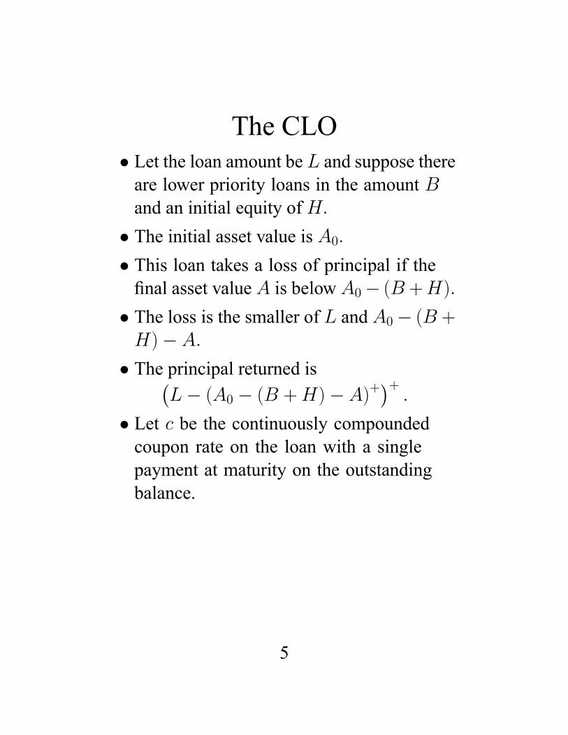
The CLO• Let the loan amount be L and suppose thereare lower priority loans in the amount Band an initial equity ofH.

• The initial asset value is A0.• This loan takes a loss of principal if thefinal asset value A is belowA0− (B +H).

• The loss is the smaller of L and A0− (B +H)−A.

• The principal returned is¡L− (A0 − (B +H)−A)+

¢+.

• Let c be the continuously compoundedcoupon rate on the loan with a singlepayment at maturity on the outstandingbalance.

5

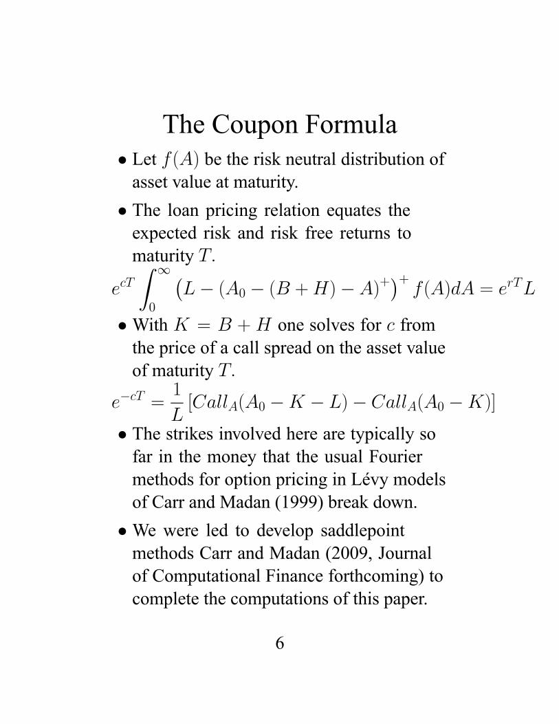
The Coupon Formula• Let f(A) be the risk neutral distribution ofasset value at maturity.

• The loan pricing relation equates theexpected risk and risk free returns tomaturity T.

ecTZ ∞0

¡L− (A0 − (B +H)−A)+

¢+f(A)dA = erTL

•With K = B + H one solves for c fromthe price of a call spread on the asset valueof maturity T.

e−cT =1

L[CallA(A0 −K − L)− CallA(A0 −K)]

• The strikes involved here are typically sofar in the money that the usual Fouriermethods for option pricing in Lévy modelsof Carr and Madan (1999) break down.

•We were led to develop saddlepointmethods Carr and Madan (2009, Journalof Computational Finance forthcoming) tocomplete the computations of this paper.

6

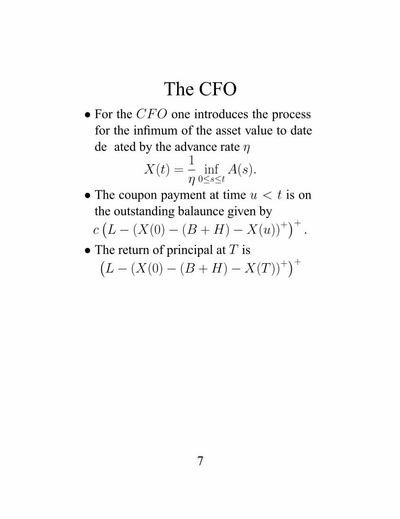
The CFO• For the CFO one introduces the processfor the infimum of the asset value to datede�ated by the advance rate η

X(t) =1

ηinf0≤s≤t

A(s).

• The coupon payment at time u < t is onthe outstanding balaunce given byc¡L− (X(0)− (B +H)−X(u))+

¢+.

• The return of principal at T is¡L− (X(0)− (B +H)−X(T ))+

¢+

7

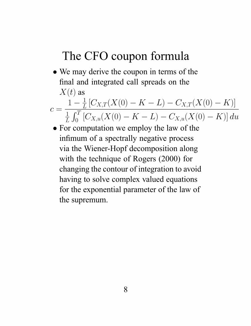
The CFO coupon formula•We may derive the coupon in terms of thefinal and integrated call spreads on theX(t) as

c =1− 1

L [CX,T (X(0)−K − L)− CX,T (X(0)−K)]1L

R T

0 [CX,u(X(0)−K − L)− CX,u(X(0)−K)] du

• For computation we employ the law of theinfimum of a spectrally negative processvia the Wiener-Hopf decomposition alongwith the technique of Rogers (2000) forchanging the contour of integration to avoidhaving to solve complex valued equationsfor the exponential parameter of the law ofthe supremum.

8

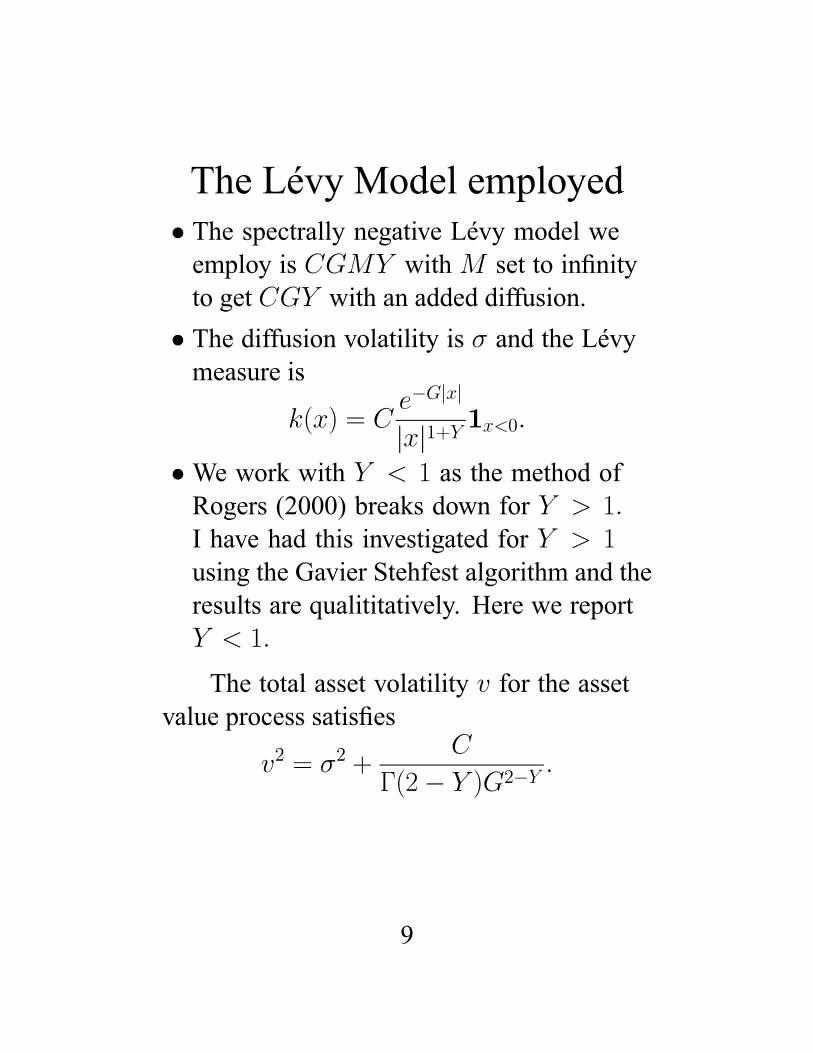
The Lévy Model employed• The spectrally negative Lévy model weemploy is CGMY withM set to infinityto get CGY with an added diffusion.

• The diffusion volatility is σ and the Lévymeasure is

k(x) = Ce−G|x|

|x|1+Y 1x<0.•We work with Y < 1 as the method ofRogers (2000) breaks down for Y > 1.I have had this investigated for Y > 1using the Gavier Stehfest algorithm and theresults are qualititatively. Here we reportY < 1.

The total asset volatility v for the assetvalue process satisfies

v2 = σ2 +C

Γ(2− Y )G2−Y.

9

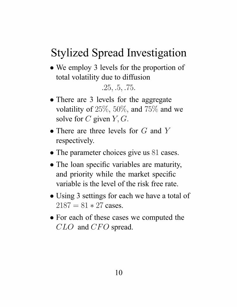
Stylized Spread Investigation•We employ 3 levels for the proportion oftotal volatility due to diffusion

.25, .5, .75.

• There are 3 levels for the aggregatevolatility of 25%, 50%, and 75% and wesolve for C given Y,G.

• There are three levels for G and Yrespectively.

• The parameter choices give us 81 cases.• The loan specific variables are maturity,and priority while the market specificvariable is the level of the risk free rate.

• Using 3 settings for each we have a total of2187 = 81 ∗ 27 cases.

• For each of these cases we computed theCLO and CFO spread.

10

Design of Fixed EffectRegression

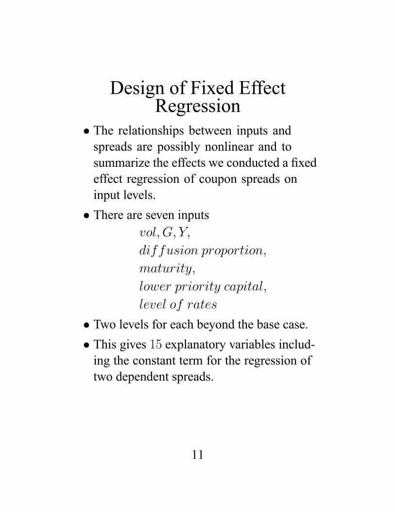
• The relationships between inputs andspreads are possibly nonlinear and tosummarize the effects we conducted a fixedeffect regression of coupon spreads oninput levels.

• There are seven inputsvol,G, Y,

diffusion proportion,

maturity,

lower priority capital,

level of rates

• Two levels for each beyond the base case.• This gives 15 explanatory variables includ-ing the constant term for the regression oftwo dependent spreads.

11

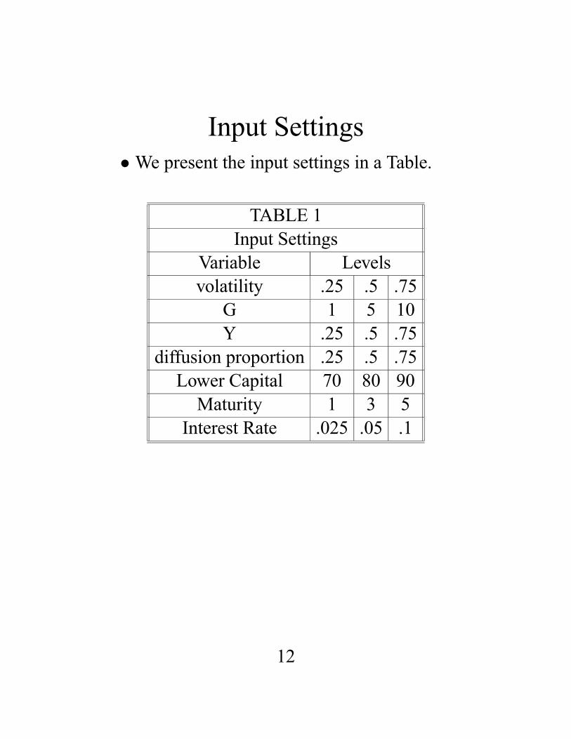
Input Settings•We present the input settings in a Table.

TABLE 1Input Settings

Variable Levelsvolatility .25 .5 .75G 1 5 10Y .25 .5 .75

diffusion proportion .25 .5 .75Lower Capital 70 80 90Maturity 1 3 5

Interest Rate .025 .05 .1

12

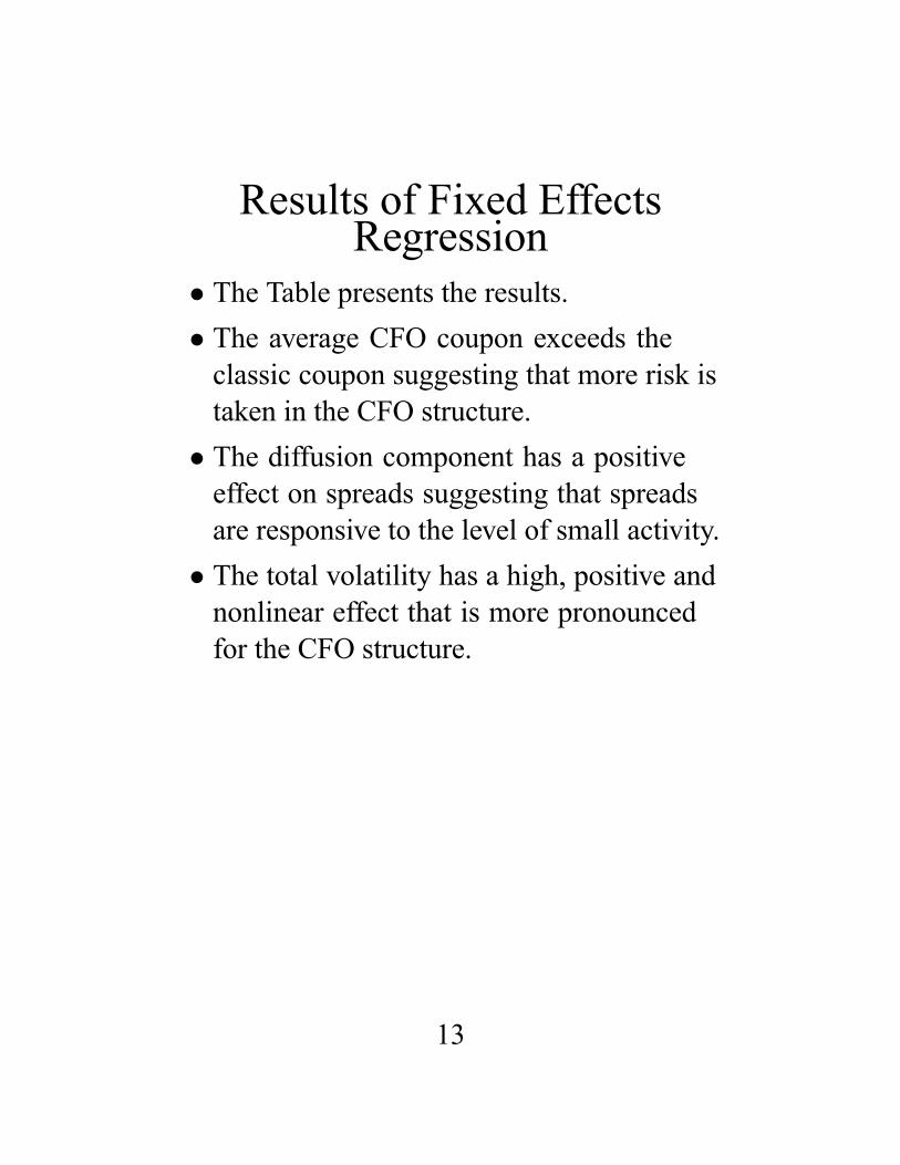
Results of Fixed EffectsRegression

• The Table presents the results.• The average CFO coupon exceeds theclassic coupon suggesting that more risk istaken in the CFO structure.

• The diffusion component has a positiveeffect on spreads suggesting that spreadsare responsive to the level of small activity.

• The total volatility has a high, positive andnonlinear effect that is more pronouncedfor the CFO structure.

13

• Interestingly, the effect of raising Gwhich increases the relative size of thesmall activity has a positive effect that isrelatively linear. This also suggests thatthe cumulated effects of small jumps areimportant.

• The effect of increasing Y are positive.This again suggests that raising the level ofsmall activity raises spreads.

14

• The effect of higher priority is negative asexpected, nonlinear and more pronouncedfor the CFO structure.

• The effects of maturity are positive, slightlynonlinear, and more pronounced for theCFO structures.

• Interestingly, lower interest rate environ-ments necessitate larger spreads.

15

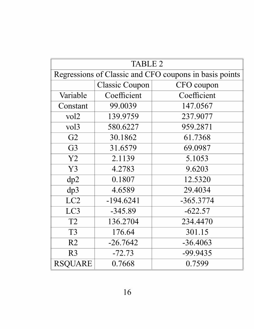
TABLE 2Regressions of Classic and CFO coupons in basis points

Classic Coupon CFO couponVariable Coefficient CoefficientConstant 99.0039 147.0567vol2 139.9759 237.9077vol3 580.6227 959.2871G2 30.1862 61.7368G3 31.6579 69.0987Y2 2.1139 5.1053Y3 4.2783 9.6203dp2 0.1807 12.5320dp3 4.6589 29.4034LC2 -194.6241 -365.3774LC3 -345.89 -622.57T2 136.2704 234.4470T3 176.64 301.15R2 -26.7642 -36.4063R3 -72.73 -99.9435

RSQUARE 0.7668 0.7599

16

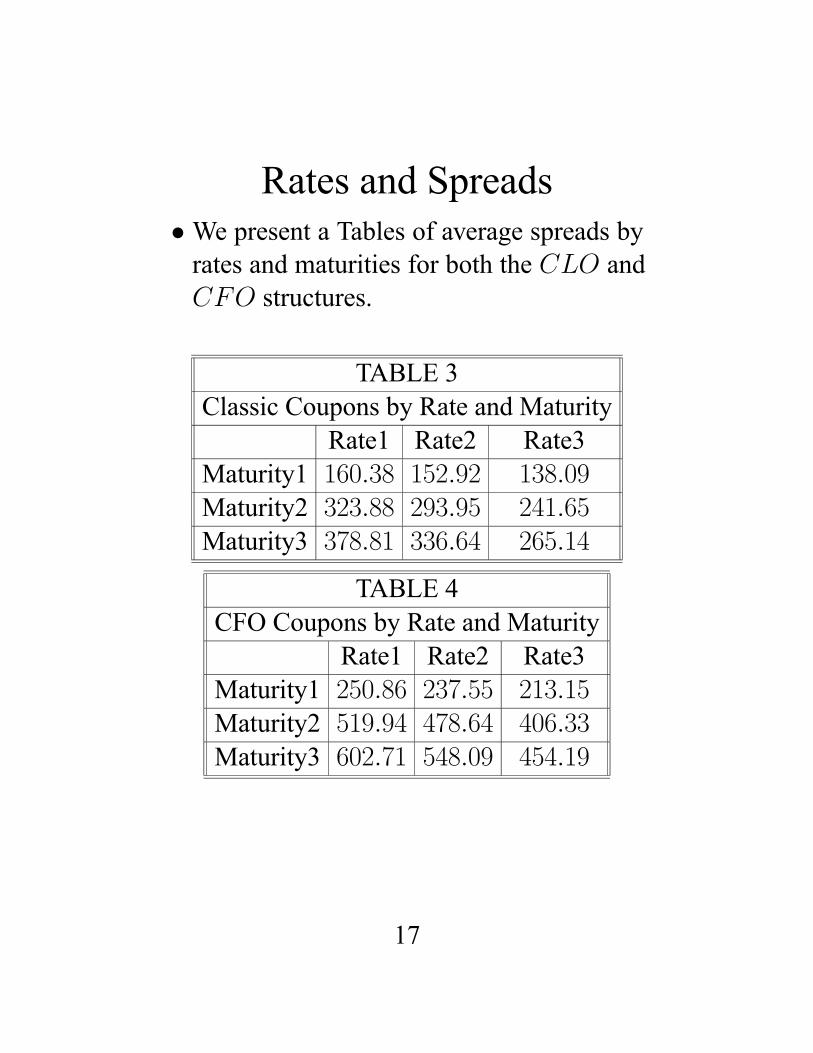
Rates and Spreads•We present a Tables of average spreads byrates and maturities for both the CLO andCFO structures.

TABLE 3Classic Coupons by Rate and Maturity

Rate1 Rate2 Rate3Maturity1 160.38 152.92 138.09Maturity2 323.88 293.95 241.65Maturity3 378.81 336.64 265.14

TABLE 4CFO Coupons by Rate and Maturity

Rate1 Rate2 Rate3Maturity1 250.86 237.55 213.15Maturity2 519.94 478.64 406.33Maturity3 602.71 548.09 454.19

17

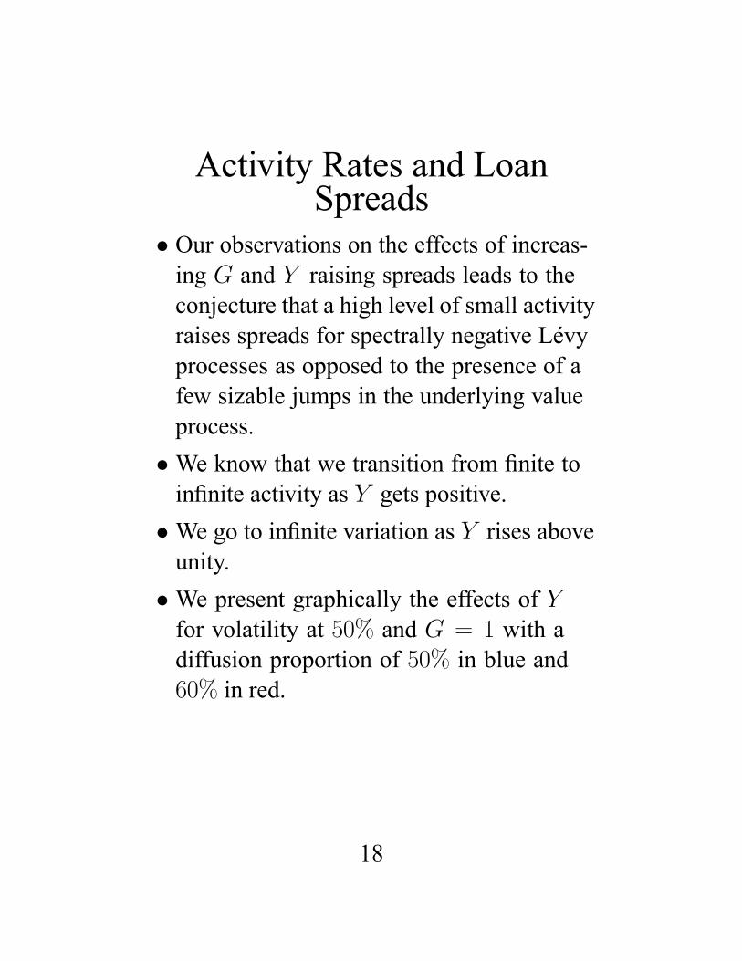
Activity Rates and LoanSpreads

• Our observations on the effects of increas-ing G and Y raising spreads leads to theconjecture that a high level of small activityraises spreads for spectrally negative Lévyprocesses as opposed to the presence of afew sizable jumps in the underlying valueprocess.

•We know that we transition from finite toinfinite activity as Y gets positive.

•We go to infinite variation as Y rises aboveunity.

•We present graphically the effects of Yfor volatility at 50% and G = 1 with adiffusion proportion of 50% in blue and60% in red.

18

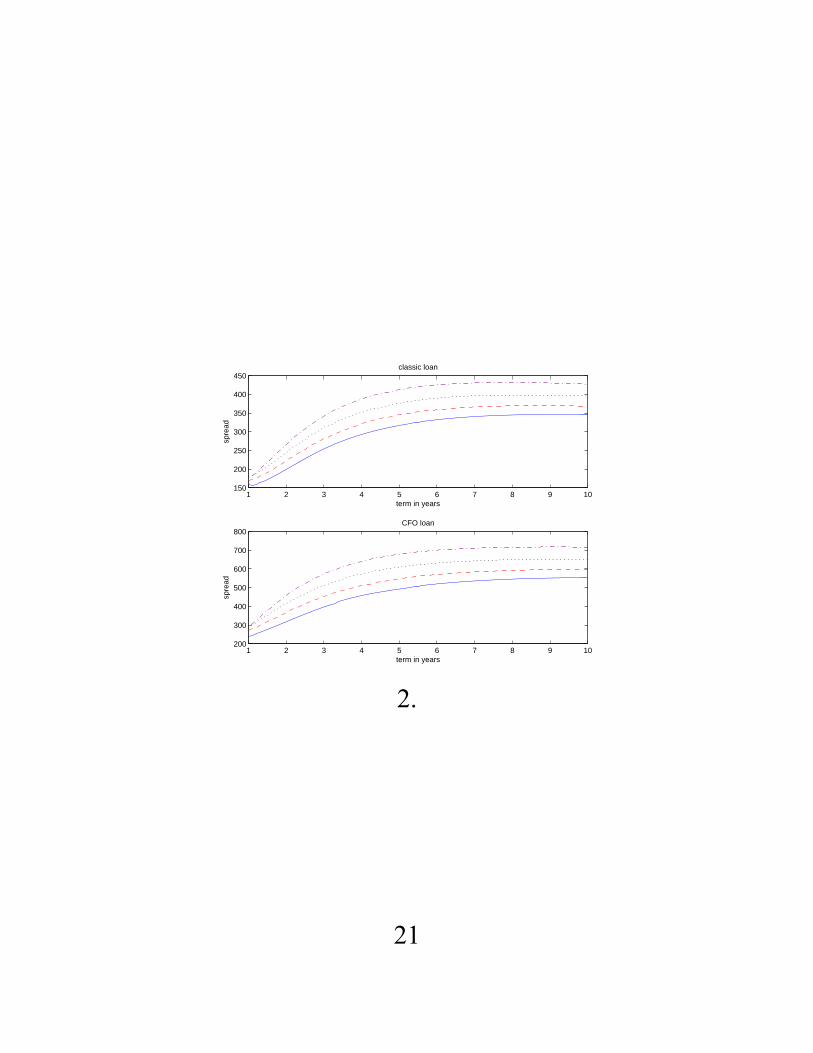
•We also present the term structure effectsof Y using four settings and graphingagainst maturity. The Y settings are−0.75,−0.25, 0.25, 0.75.

19

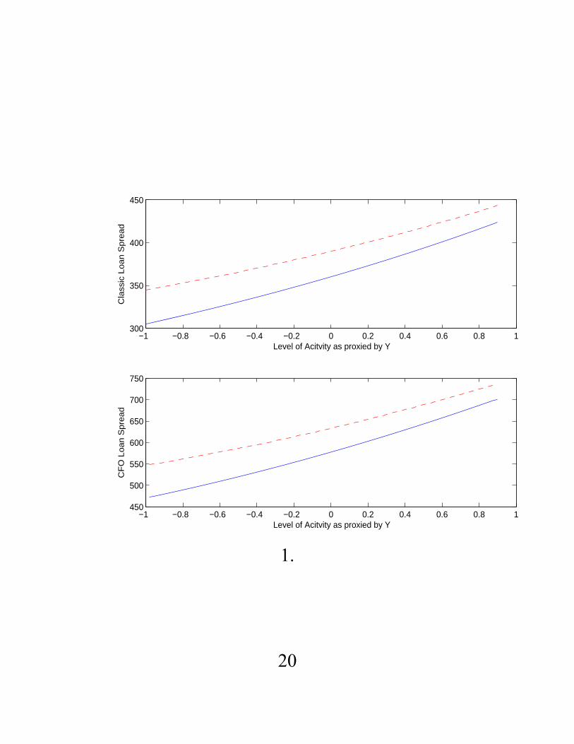
−1 −0.8 −0.6 −0.4 −0.2 0 0.2 0.4 0.6 0.8 1300

350

400

450

Level of Acitvity as proxied by Y

Cla

ssic

Loan S

pre

ad

−1 −0.8 −0.6 −0.4 −0.2 0 0.2 0.4 0.6 0.8 1450

500

550

600

650

700

750

Level of Acitvity as proxied by Y

CF

O L

oan S

pre

ad

1.

20

1 2 3 4 5 6 7 8 9 10150

200

250

300

350

400

450classic loan

term in years

spre

ad

1 2 3 4 5 6 7 8 9 10200

300

400

500

600

700

800CFO loan

term in years

spre

ad

2.

21

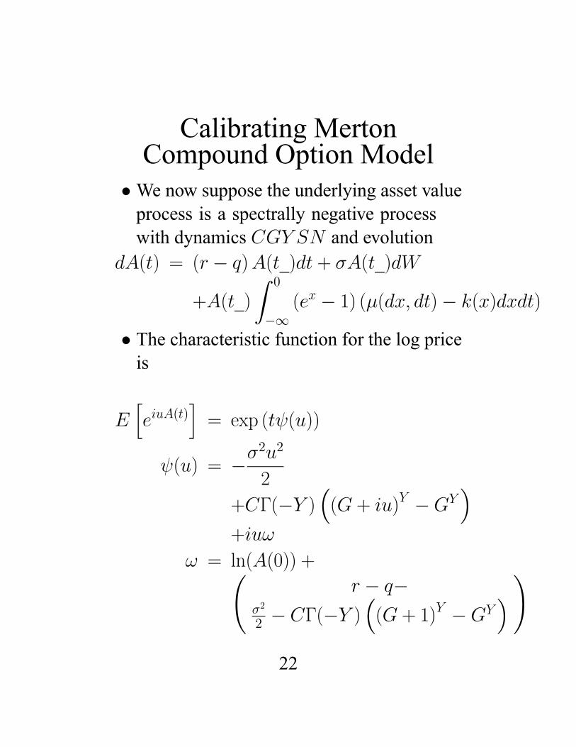
Calibrating MertonCompound Option Model

•We now suppose the underlying asset valueprocess is a spectrally negative processwith dynamics CGY SN and evolution

dA(t) = (r − q)A(t_)dt + σA(t_)dW

+A(t_)Z 0

−∞(ex − 1) (μ(dx, dt)− k(x)dxdt)

• The characteristic function for the log priceis

EheiuA(t)

i= exp (tψ(u))

ψ(u) = −σ2u2

2

+CΓ(−Y )³(G + iu)Y −GY

´+iuω

ω = ln(A(0)) +Ãr − q−

σ2

2 − CΓ(−Y )³(G+ 1)Y −GY

´ !

22

•We take the debt level of the companyas the strike and the debt maturity as thematurity and solve for asset value using

S0 = C(A0, D,M ;σ,C,G, Y )

• where S0 is the market stock price. Hencethe stock is a call option on the asset value.

•We calibrate the parameters σ,C,G, Y tofit the equity option surface. We simulatethe asset value process from a prospectiveset of parameters and transform to stockprices usingS(t) = C(A(t), D,M ;σ,C,G, Y )

•We then price options on the path spaceand match these with traded market optionprices.

• The estimated model is then used to priceloan spreads of both types for the saidcompany on the stated date.

23

Illustration on GM 2003• The Debt level for 2003 was 191, 133millions of dollars.

• The outstanding equity was 25, 268millionsof dollars.

• The stock price averaged over December2003 was 49.44.

• The implied number of shares was 511.1076million shares.

•We set the asset value strike at the debtlevel per share of 373.9584.

• The maturity was set at the period durationof 12 years.

24

• The average option surface for December2003 was synthesized by V GSSD Satoprocess parameters of

σ = .2803, ν = .9027, θ = −.1131, γ = .5314.

• From these parameter values and initialstock price of 49.44we build a target optionprice surface using 36 prices with 9 strikesfor each of four maturities.

25

•We calibrate the asset value process tothese option prices using our simulatedcompound option pricing model.

• The parameter values wereσ = .0.0189, C = 0.2297, G = 1.0991, Y = 0.3604

26

•We also did a standard equity optioncalibration of the CGY SN model toequity option prices to get parameters

σ = 0.2064, C = 0.0956, G = 1.1818, Y = 0.4953

•We then computed loan spreads for 70%lower priority capital for the 5 year CLOand CFO.

27

CLO and CFO Loan Spreadson GM 2003

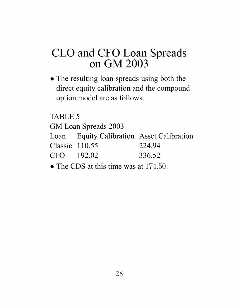
• The resulting loan spreads using both thedirect equity calibration and the compoundoption model are as follows.

TABLE 5GM Loan Spreads 2003Loan Equity Calibration Asset CalibrationClassic 110.55 224.94CFO 192.02 336.52• The CDS at this time was at 174.50.

28

Conclusion• Classic loan spreads for spectrally negativeLévy processes are implemented by callspread calculations using new saddlepointmethods of Carr and Madan (2009).

• CFO loan spread computations are doneusing Rogers (2000).

• It is observed that the level of small jumpactivity strongly in�uences the level ofspreads in addition to other factors.

• The Merton compound option model isused to calibrate asset value parameters toan equity option surface to infer asset valueparameters

• Loan spread computations are then illus-trated for both loan types using calibartedparameters.

29