RISK, UNCERTAINTY AND MONETARY POLICY … · Risk, Uncertainty and Monetary Policy Geert Bekaert,...

NBER WORKING PAPER SERIES

RISK, UNCERTAINTY AND MONETARY POLICY

Geert BekaertMarie HoerovaMarco Lo Duca

Working Paper 16397http://www.nber.org/papers/w16397

NATIONAL BUREAU OF ECONOMIC RESEARCH1050 Massachusetts Avenue

Cambridge, MA 02138September 2010

We thank Gianni Amisano, Bartosz Mackowiak, Frank Smets, José Valentim and seminar participantsat the European Central Bank, the FRB Philadelphia, the 2010 Midwest Macroeconomics Meetings(East Lansing) and the Fifth Annual Seminar on Banking, Financial Stability and Risk (Sao Paulo)for helpful comments and suggestions. Falk Bräuning and Francesca Fabbri provided excellent researchassistance. The views expressed do not necessarily reflect those of the European Central Bank, theEurosystem, or the National Bureau of Economic Research.

NBER working papers are circulated for discussion and comment purposes. They have not been peer-reviewed or been subject to the review by the NBER Board of Directors that accompanies officialNBER publications.

© 2010 by Geert Bekaert, Marie Hoerova, and Marco Lo Duca. All rights reserved. Short sectionsof text, not to exceed two paragraphs, may be quoted without explicit permission provided that fullcredit, including © notice, is given to the source.

Risk, Uncertainty and Monetary PolicyGeert Bekaert, Marie Hoerova, and Marco Lo DucaNBER Working Paper No. 16397September 2010, Revised July 2012JEL No. E32,E44,E52,G12

ABSTRACT

The VIX, the stock market option-based implied volatility, strongly co-moves with measures of themonetary policy stance. When decomposing the VIX into two components, a proxy for risk aversionand expected stock market volatility (“uncertainty”), we find that a lax monetary policy decreasesboth risk aversion and uncertainty, with the former effect being stronger. The result holds in a structuralvector autoregressive framework, controlling for business cycle movements and using a variety ofidentification schemes for the vector autoregression in general and monetary policy shocks in particular.

Geert BekaertGraduate School of BusinessColumbia University3022 Broadway, 411 Uris HallNew York, NY 10027and [email protected]

Marie HoerovaEuropean Central BankKaiserstrasse 29 D-60311Frankfurt am Main, [email protected]

Marco Lo DucaEuropean Central BankKaiserstrasse 29 D-60311Frankfurt am Main, [email protected]

1

1. Introduction

A popular indicator of risk aversion in financial markets, the VIX index, shows strong

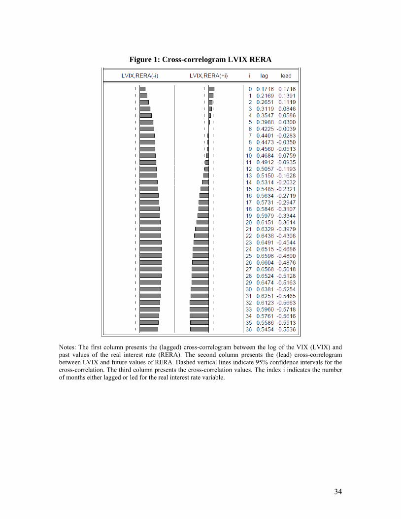
co-movements with measures of the monetary policy stance. Figure 1 considers the cross-

correlogram between the real interest rate (the Fed funds rate minus inflation), a measure

of the monetary policy stance, and the logarithm of end-of-month readings of the VIX

index. The VIX index essentially measures the “risk-neutral” expected stock market

variance for the US S&P500 index. The correlogram reveals a very strong positive

correlation between real interest rates and future VIX levels. While the current VIX is

positively associated with future real rates, the relationship turns negative and significant

after 13 months: high VIX readings are correlated with expansionary monetary policy in

the medium-run future.

The strong interaction between a “fear index” (Whaley (2000)) in the asset markets

and monetary policy indicators may have important implications for a number of

literatures. First, the recent crisis has rekindled the idea that lax monetary policy can be

conducive to financial instability. The Federal Reserve’s pattern of providing liquidity to

financial markets following market tensions, which became known as the “Greenspan

put,” has been cited as one of the contributing factors to the build-up of a speculative

bubble prior to the 2007-09 financial crisis.1 Whereas some rather informal stories have

linked monetary policy to risk-taking in financial markets (Rajan (2006), Adrian and Shin

1 Investors increasingly believed that when market conditions were to deteriorate, the Fed would step in and inject liquidity until the outlook improved. Such perception may encourage excessive risk-taking and lead to higher valuations and narrower credit spreads. See, for example, “Greenspan Put may be Encouraging Complacency,” Financial Times, December 8, 2000.

http://en.wikipedia.org/wiki/Speculative_bubble

http://en.wikipedia.org/wiki/Speculative_bubble

http://en.wikipedia.org/wiki/Financial_crisis_of_2007%E2%80%932009

2

(2008), Borio and Zhu (2008)), it is fair to say that no extant research establishes a firm

empirical link between monetary policy and risk aversion in asset markets.2

Second, Bloom (2009) and Bloom, Floetotto and Jaimovich (2009) show that

heightened “economic uncertainty” decreases employment and output. It is therefore

conceivable that the monetary authority responds to uncertainty shocks, in order to affect

economic outcomes. However, the VIX index, used by Bloom (2009) to measure

uncertainty, can be decomposed into a component that reflects actual expected stock

market volatility (uncertainty) and a residual, the so-called variance premium (see, for

example, Carr and Wu (2009)), that reflects risk aversion and other non-linear pricing

effects, perhaps even Knightian uncertainty. Establishing which component drives the

strong co-movements between the monetary policy stance and the VIX is therefore

particularly important.

Third, analyzing the relationship between monetary policy and the VIX and its

components may help clarify the relationship between monetary policy and the stock

market, explored in a large number of empirical papers (Thorbecke (1997), Rigobon and

Sack (2004), Bernanke and Kuttner (2005)). The extant studies all find that expansionary

(contractionary) monetary policy affects the stock market positively (negatively).

Interestingly, Bernanke and Kuttner (2005) ascribe the bulk of the effect to easier

monetary policy lowering risk premiums, reflecting both a reduction in economic and

financial volatility and an increase in the capacity of financial investors to bear risk. By

using the VIX and its two components, we test the effect of monetary policy on stock

market risk, but also provide more precise information on the exact channel.

2 For recent empirical evidence that monetary policy affects the riskiness of loans granted by banks see, for example, Altunbas, Gambacorta and Marquéz-Ibañez (2010), Ioannidou, Ongena and Peydró (2009), Jiménez, Ongena, Peydró and Saurina (2009), and Maddaloni and Peydró (2010).

3

This article characterizes the dynamic links between risk aversion, economic

uncertainty and monetary policy in a simple vector-autoregressive (VAR) system. Such

analysis faces a number of difficulties. First, because risk aversion and the stance of

monetary policy are jointly endogenous variables and display strong contemporaneous

correlation (see Figure 1), a structural interpretation of the dynamic effects requires

identifying restrictions. Monetary policy may indeed affect asset prices through its effect

on risk aversion, as suggested by the literature on monetary policy news and the stock

market, but monetary policy makers may also react to a nervous and uncertain market

place by loosening monetary policy. In fact, Rigobon and Sack (2003) find that the

Federal Reserve does systematically respond to stock prices.3

Second, the relationship between risk aversion and monetary policy may also reflect

the joint response to an omitted variable, with business cycle variation being a prime

candidate. Recessions may be associated with high risk aversion (see Campbell and

Cochrane (1999) for a model generating counter-cyclical risk aversion) and at the same

time lead to lax monetary policy. Our VARs always include a business cycle indicator.

Third, measuring the monetary policy stance is the subject of a large literature (see,

for example, Bernanke and Mihov (1998a)); and measuring policy shocks correctly is

difficult. Models featuring time-varying risk aversion and/or uncertainty, such as Bekaert,

Engstrom and Xing (2009), imply an equilibrium contemporaneous link between interest

rates and risk aversion and uncertainty, through precautionary savings effects for

example. Such relation should not be associated with a policy shock. However, our

3 The two papers by Rigobon and Sack (2003, 2004) use an identification scheme based on the heteroskedasticity of stock market returns. Given that we view economic uncertainty as an important endogenous variable in its own right with links to the real economy and risk premiums, we cannot use such an identification scheme.

4

results are robust to alternative measures of the monetary policy stance and of monetary

policy shocks. In particular, the results are robust to identifying monetary policy shocks

using a standard structural VAR, high frequency Fed funds futures changes following

Gürkaynak, Sack and Swanson (2005), and monthly surprises based on the daily Fed

funds futures following the approach in Bernanke and Kuttner (2005).

The remainder of the paper is organized as follows. In Section 2, we detail the

measurement of the key variables in the VAR, including monetary policy indicators,

monetary policy shocks and business cycle indicators. First and foremost, we provide

intuition on how the VIX is related to the actual expected variance of stock returns and to

risk preferences. While the literature has proposed a number of risk appetite measures

(see Baker and Wurgler (2007) and Coudert and Gex (2008)), our measure is

monotonically increasing in risk aversion in a variety of economic settings. This

motivates our empirical strategy in which we split the VIX into a pure volatility

component (“uncertainty”) and a residual, which should be more closely associated with

risk aversion. In Section 3, we analyze the dynamic relationship between monetary policy

and risk aversion and uncertainty in standard structural VARs. The results are remarkably

robust to a long list of robustness checks with respect to VAR specification, variable

definitions and alternative identification methods. In Section 4, we use two alternative

methods to identify monetary policy shocks relying on Fed futures data.

Our main findings are as follows. A lax monetary policy decreases risk aversion in

the stock market after about nine months. This effect is persistent, lasting for more than

two years. Moreover, monetary policy shocks account for a significant proportion of the

variance of risk aversion. The effects of monetary policy on uncertainty are similar but

5

somewhat weaker. On the other hand, periods of both high uncertainty and high risk

aversion are followed by a looser monetary policy stance but these results are less robust

and much weaker statistically. Finally, it is the uncertainty component of the VIX that has

the statistically stronger effect on the business cycle, not the risk aversion component.

2. Measurement

This section details the measurement of the key inputs to our analysis: risk aversion

and uncertainty; the monetary policy stance and monetary policy shocks; and finally,

business cycle variation. Our data start in January 1990 (the start of the model-free VIX

series) but we perform our analysis using two different end-points for the sample: July

2007, yielding a sample that excludes recent data on the crisis; and August 2010. The

crisis period presents special challenges as stock market volatilities peaked at

unprecedented levels and the Fed funds target rate reached the zero lower bound. We

detail how we address these challenges below. Table 1 describes the basic variables we

use and assigns them a short-hand label.

2.1 Measuring Risk Aversion and Uncertainty

To measure risk aversion and uncertainty, we use a decomposition of the VIX index.

The VIX represents the option-implied expected volatility on the S&P500 index with a

horizon of 30 calendar days (22 trading days). This volatility concept is often referred to

as “implied volatility” or “risk-neutral volatility,” as opposed to the actual (or “physical”)

expected volatility. Intuitively, in a discrete state economy, the physical volatility would

use the actual state probabilities to arrive at the physical expected variance, whereas the

risk-neutral variance would make use of probabilities that are adjusted for the pricing of

risk.

6

The computation of the actual VIX index relies on theoretical results showing that

option prices can be used to replicate any bounded payoff pattern; in fact, they can be

used to replicate Arrow-Debreu securities (Breeden and Litzenberger (1978), Bakshi and

Madan (2000)). Britten-Jones and Neuberger (2000) and Bakshi, Kapadia and Madan

(2003) show how to infer “risk-neutral” expected volatility for a stock index from option

prices. The VIX index measures implied volatility using a weighted average of European-

style S&P500 call and put option prices that straddle a 30-day maturity and cover a wide

range of strikes (see CBOE (2004) for more details). Importantly, this estimate is model-

free and does not rely on an option pricing model.

While the VIX obviously reflects stock market uncertainty, it conceptually must also

harbor information about risk and risk aversion. Indeed, financial markets often view the

VIX as a measure of risk aversion and fear in the market place. Because there are well-

accepted techniques to measure the physical expected variance, we can split the VIX into

a measure of stock market or economic uncertainty, and a residual that should be more

closely associated with risk aversion. The difference between the squared VIX and an

estimate of the conditional variance is typically called the variance premium (see, e.g.,

Carr and Wu (2009)).4 The variance premium is nearly always positive and displays

substantial time-variation. Recent finance models attribute these facts either to non-

Gaussian components in fundamentals and (stochastic) risk aversion (see, for instance,

Bekaert and Engstrom (2010), Bollerslev, Tauchen and Zhou (2009), Drechsler and

Yaron (2011)) or Knightian uncertainty (see Drechsler (2009)). In the Appendix, we use

a one-period discrete economy with power utility to illustrate the difference between

4 In the technical finance literature, the variance premium is actually the negative of the variable that we use. By switching the sign, our indicator increases with risk aversion, whereas the variance premium becomes more negative with risk aversion.

7

“risk neutral” and “physical” expected volatility and demonstrate that the variance

premium is indeed increasing in risk aversion.

To decompose the VIX index into a risk aversion and an uncertainty component, we

first estimate the expected future realized variance. It is customary in the literature to do

so by projecting future realized monthly variances (computed using squared 5-minute

returns) onto a set of current instruments. We follow this approach using daily data on

monthly realized variances, the squared VIX, the dividend yield and the real three-month

T-bill rate. By using daily data, we gain considerable statistical power relative to the

standard methods employing end-of-month data. For example, forecasting models

estimated from daily data easily “beat” models using only end-of-month data, even for

end-of-month samples.

To select a good forecasting model, we conduct a horserace between a total of eight

volatility forecasting models. The first five models use OLS regressions with different

predictors: a one-variable model with either the past realized variance or the squared

VIX; a two-variable model with both the squared VIX and the past realized variance; a

three-variable model adding the past dividend yield; and a four-variable model adding the

past real three-month T-bill rate. We also consider three models that do not require

estimation: half-half weights on the past squared VIX and past realized variance; the past

realized variance; the past squared VIX. We consider two model selection criteria: out-

of-sample root-mean-squared error and mean absolute errors, and, for the estimated

models, stability (especially through the crisis period).

This procedure leads us to select a two-variable model where the squared VIX and the

past realized variance are used as predictors. The performance of the three and four

8

variable models is very comparable to this model, but the univariate estimated models

and the non-estimated models perform consistently and significantly worse. Moreover,

the model that we selected is the most stable of the well-performing forecasting models

we considered, with the coefficients economically and statistically unaltered during the

crisis period. In the online Appendix, we give a detailed account of the forecasting

horserace. The resulting coefficients from the two-variable projection are as follows:5

RVARt=-0.00002 + 0.299 VIX2t-22 + 0.442 RVARt-22+et (1)

(0.00012) (0.067) (0.130)

The standard errors reported in parentheses are corrected for serial correlation using 30

Newey-West (1987) lags.

The fitted value from the two-variable projection is the estimated physical expected

variance (“uncertainty”). We use the logarithm of this estimate in our analysis and label it

UC. We call the difference between the squared VIX and UC “risk aversion” (the

logarithm of which is labeled as RA). We plot the risk aversion and uncertainty estimates

in Figure 2, along with 90% confidence intervals.6 To construct the confidence bounds,

we retain the coefficients from the forecasting projection together with their asymptotic

covariance matrix. We then draw 100 alternative parameter coefficients from the

distribution of these estimates, which generates alternative RA and UC estimates. In

Section 3.2.4, we use these bootstrapped series to account for the sampling error in the

risk aversion and uncertainty estimates in our VARs.

2.2 Measuring Monetary Policy

5 This estimation was conducted using a winsorized sample but the estimation results for the non-winsorized sample are in fact very similar. 6 The estimated uncertainty series is less “jaggedy” than it would be if only the past realized variance would be used to compute it (as in Bollerslev, Tauchen and Zhou, 2009), which in turn helps smooth the risk aversion process.

9

To measure the monetary policy stance, we use the real interest rate (RERA), i.e., the

Fed funds end-of-the-month target rate minus the CPI annual inflation rate. In Section

3.2.1, we consider alternative measures of the monetary policy stance for robustness. Our

first such measure is the Taylor rule residual, the difference between the nominal Fed

funds rate and the Taylor rule rate (TR rate). The TR rate is estimated as in Taylor

(1993):

TRt = Inft + NatRatet + 0.5 (Inft - TargInf) + 0.5 OGt (2)

where Inf is the annual inflation rate, NatRate is the “natural” real Fed funds rate

(consistent with full employment), which Taylor assumed to be 2%, TargInf is a target

inflation rate, also assumed to be 2%, and OG (output gap) is the percentage deviation of

real GDP from potential GDP; with the latter obtained from the Congressional Budget

Office. As other alternative measures of the monetary policy stance, we consider the

nominal Fed funds rate instead of the real rate, and (the growth rate of) the monetary

aggregate M1, which is commonly assumed to be under tight control of the central bank.

We multiply M1 (growth) by minus one so that a positive shock to this variable

corresponds to monetary policy tightening, in line with all other measures of monetary

policy we use.

Measuring the monetary policy stance is challenging since late 2008, as the Fed funds

rate reached the zero lower bound (the Fed funds target was set in the range 0-0.25% as

of December 2008) and the Federal Reserve turned to unconventional monetary policies,

such as large-scale asset purchases. We approximate the “true” nominal Fed funds rate in

the period December 2008 - August 2010 by taking it to be the minimum between

0.125% (i.e., the mid-point of the 0-0.25% range) and the TR rate, estimated using

10

equation (2) above. Rudebusch (2009) has also advocated using the TR rate estimate as a

proxy for the “true” Fed funds rate post-2008.

In our analysis in Sections 4.1 and 4.2, we use monetary policy surprises derived

from Fed funds futures data. In Section 4.1, we rely on monetary policy surprises

proposed by Gürkaynak, Sack and Swanson (2005), henceforth GSS.7 GSS compute the

monetary policy surprises as high-frequency changes in the futures rate around the

FOMC announcements. Their “tight” (“wide”) window estimates begin ten (fifteen)

minutes prior to the monetary policy announcement and end twenty (forty-five) minutes

after the policy announcement, respectively. The data span the period from January 1990

through June 2008. In Section 4.2, we use the unexpected change in the Fed funds rate on

a monthly basis, defined as the average Fed funds target rate in month t minus the one-

month futures rate on the last day of the month t-1. This approach follows Kuttner (2001)

and Bernanke and Kuttner (2005) (henceforth BK); see their equation (5). As pointed out

by BK, rate changes that were unanticipated as of the end of the prior month may well

include a systematic response to economic news, such as employment, output and

inflation occurring during the month. To overcome this problem, we calculate “cleansed”

monetary surprises that are orthogonal to a set of economic data releases. They are

calculated as residuals in a regression of the “simple” monetary policy surprise, onto the

unexpected component of the industrial production index, the Institute of Supply

Management Purchasing Managers Index (the ISM index), the payroll survey, and

unemployment (see Section 2.3 below for a description). Finally, in the regression, we

allow for heterogeneous coefficients before and after 1994, to take into account a change

in the reaction of the Fed to economic data releases, as documented in BK. 7 We are very grateful to R. Gürkaynak for sharing the data with us.

11

To extend the sample of monetary policy surprises until August 2010, we proceed in

two steps. First, we collect data on monetary policy surprises at the zero lower bound

from Wright (2011, Table 5). The surprises are based on a structural VAR in financial

variables at the daily frequency, starting in November 2008 (and calculated beyond the

end of our sample in August 2010). The shocks are positive (negative) when monetary

policy is unexpectedly accommodative (restrictive). They also have a standard deviation

equal to one by construction. For comparability with the GSS data, we rescale Wright’s

shocks by multiplying them by minus the standard deviation of the GSS’s shocks, before

appending them to the time series of GSS shocks. Second, to fill the gap between the data

from GSS (June 2008) and Wright (November 2008), we calculate monetary policy

surprises using Federal funds futures, following BK.

2.3 Measuring Business Cycle Variation

We use industrial production as our benchmark indicator of business cycle variation

at the monthly frequency. In a robustness exercise in Section 3.2.2, we also consider non-

farm employment and the ISM index as alternative business cycle indicators.

In Sections 4.1 and 4.2, we use data on economic news surprises following the

methodology in Ehrmann and Fratzscher (2004).8 In our analysis, we rely on unexpected

components of news about the industrial production index, the ISM index, the payroll

survey, and unemployment. The unexpected component of each news release is

calculated as the difference between the released data and the median expectation

according to surveys. We use the Money Market Survey (MMS) for the period 1990-

2001 and Bloomberg for the period 2002-2010. The shocks are standardized over the

sample period. 8 We are very grateful to M. Ehrmann and M. Fratzscher for sharing their dataset with us.

12

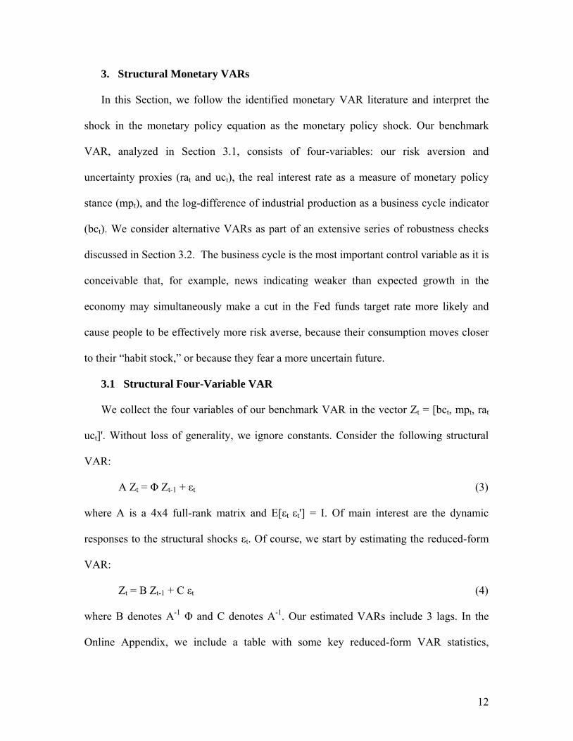
3. Structural Monetary VARs

In this Section, we follow the identified monetary VAR literature and interpret the

shock in the monetary policy equation as the monetary policy shock. Our benchmark

VAR, analyzed in Section 3.1, consists of four-variables: our risk aversion and

uncertainty proxies (rat and uct), the real interest rate as a measure of monetary policy

stance (mpt), and the log-difference of industrial production as a business cycle indicator

(bct). We consider alternative VARs as part of an extensive series of robustness checks

discussed in Section 3.2. The business cycle is the most important control variable as it is

conceivable that, for example, news indicating weaker than expected growth in the

economy may simultaneously make a cut in the Fed funds target rate more likely and

cause people to be effectively more risk averse, because their consumption moves closer

to their “habit stock,” or because they fear a more uncertain future.

3.1 Structural Four-Variable VAR

We collect the four variables of our benchmark VAR in the vector Zt = [bct, mpt, rat

uct]'. Without loss of generality, we ignore constants. Consider the following structural

VAR:

A Zt = Φ Zt-1 + εt (3)

where A is a 4x4 full-rank matrix and E[εt εt'] = I. Of main interest are the dynamic

responses to the structural shocks εt. Of course, we start by estimating the reduced-form

VAR:

Zt = B Zt-1 + C εt (4)

where B denotes A-1 Φ and C denotes A-1. Our estimated VARs include 3 lags. In the

Online Appendix, we include a table with some key reduced-form VAR statistics,

13

showing that the Schwarz criterion selects a one-lag VAR, whereas the Akaike criterion

selects three lags. Moreover, residual specification tests (Johansen, 1995) show that the

VAR with 3 lags clearly eliminates all serial correlation in the residuals.

We need 6 restrictions on the VAR to identify the system. Our first set of restrictions

uses a standard Cholesky decomposition of the estimate of the variance-covariance

matrix. We order the business cycle variable first, followed by the real interest rate, with

risk aversion and uncertainty ordered last. This captures the fact that risk aversion and

uncertainty, stock market based variables, respond instantly to monetary policy shocks,

while the business cycle variable is relatively more slow-moving. Effectively, this

imposes six exclusion restrictions on the contemporaneous matrix A, making it lower-

triangular.

Our second set of restrictions combines five contemporaneous restrictions (also

imposed under the Cholesky decomposition above) with the assumption that monetary

policy has no long-run effect on the level of industrial production. This long-run

restriction is inspired by the literature on long-run money neutrality: money should not

have a long run effect on real variables.9 Following Blanchard and Quah (1989), the

model with a long-run restriction (LR) involves a long-run response matrix, denoted by

D:

D (I - B)-1 C. (5)

The system with five contemporaneous restrictions and one long-run exclusion restriction

corresponds to the following contemporaneous matrix A and long-run matrix D:10

9 Bernanke and Mihov (1998b) and King and Watson (1992) marshal empirical evidence in favor of money neutrality using data on money growth and output growth. 10 Both identification schemes satisfy necessary and sufficient conditions for global identification of structural vector autoregressive systems (see Rubio-Ramírez, Waggoner and Zha (2010)).

14

A =

44434241

333231

2221

1211

00000

aaaa

aaa

aa

aa

and D =

44434241

34333231

24232221

141311 0

dddd

dddd

dddd

ddd

(6)

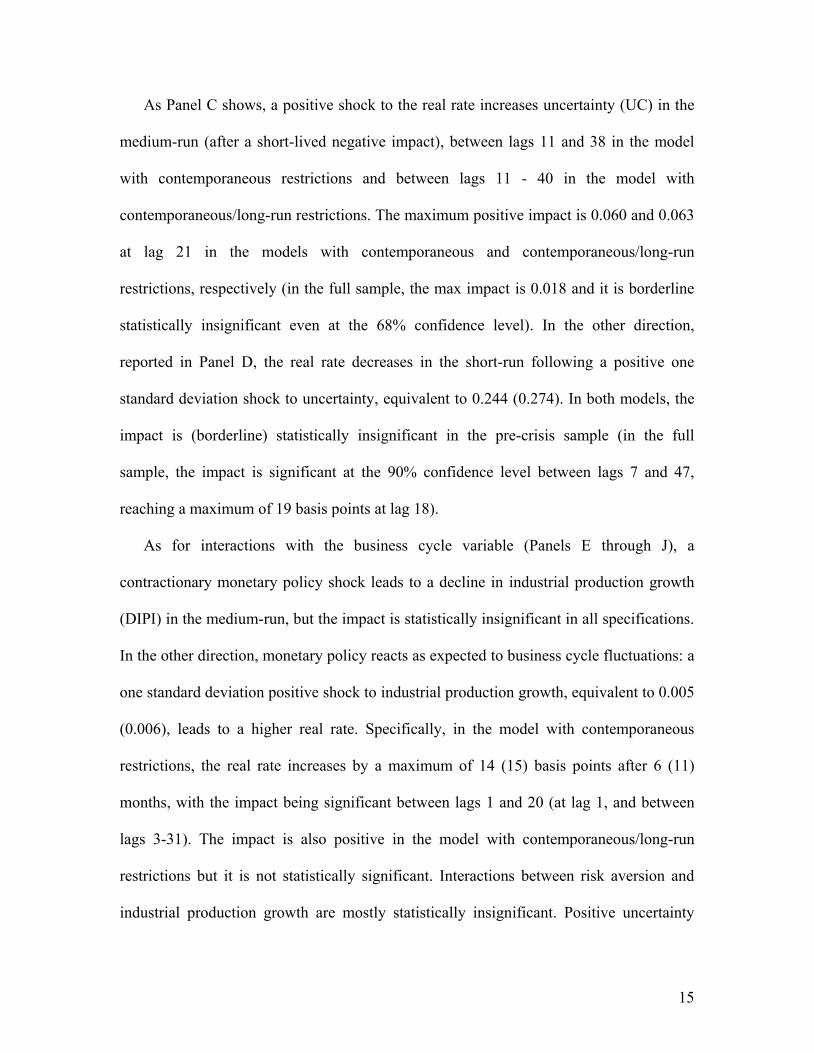
We couch our main results in the form of impulse-response functions (IRFs

henceforth), estimated in the usual way, and focus our discussion on significant

responses. We compute 90% bootstrapped confidence intervals based on 1000

replications. Figure 3 graphs the complete results for the pre-crisis sample but in our

discussion we mention the corresponding full sample (till August 2010) results in

parentheses. A complete graph for the full sample, mimicking Figure 3, is reproduced in

the Online Appendix (Figure OA1).

Panels A and B show the interactions between the real rate (RERA) and risk aversion

(RA). A one standard deviation negative shock to the real rate, a 34 (42) basis points

decrease under both identification schemes, lowers risk aversion by 0.032 (0.019) in the

model with contemporaneous restrictions and by 0.035 (0.019) in the model with

contemporaneous/long-run restrictions after 9 (19) months. The impact reaches a

maximum of 0.056 (0.020) after 20 (23) months and remains significant up and till lag 40

(40) in both models. So, laxer monetary policy lowers risk aversion under both

identification schemes and in both the pre-crisis and full samples. The impact in the full

sample is quantitatively weaker, and is only statistically significant at the 68% confidence

level. However, such tighter confidence bounds are common in the VAR literature (see

Christiano, Eichenbaum, and Evans (1996), Sims and Zha (1999)). The impact of a one

standard deviation positive shock to risk aversion, equivalent to 0.347 (0.363) on the real

rate is mostly negative but not statistically significant in both models,

15

As Panel C shows, a positive shock to the real rate increases uncertainty (UC) in the

medium-run (after a short-lived negative impact), between lags 11 and 38 in the model

with contemporaneous restrictions and between lags 11 - 40 in the model with

contemporaneous/long-run restrictions. The maximum positive impact is 0.060 and 0.063

at lag 21 in the models with contemporaneous and contemporaneous/long-run

restrictions, respectively (in the full sample, the max impact is 0.018 and it is borderline

statistically insignificant even at the 68% confidence level). In the other direction,

reported in Panel D, the real rate decreases in the short-run following a positive one

standard deviation shock to uncertainty, equivalent to 0.244 (0.274). In both models, the

impact is (borderline) statistically insignificant in the pre-crisis sample (in the full

sample, the impact is significant at the 90% confidence level between lags 7 and 47,

reaching a maximum of 19 basis points at lag 18).

As for interactions with the business cycle variable (Panels E through J), a

contractionary monetary policy shock leads to a decline in industrial production growth

(DIPI) in the medium-run, but the impact is statistically insignificant in all specifications.

In the other direction, monetary policy reacts as expected to business cycle fluctuations: a

one standard deviation positive shock to industrial production growth, equivalent to 0.005

(0.006), leads to a higher real rate. Specifically, in the model with contemporaneous

restrictions, the real rate increases by a maximum of 14 (15) basis points after 6 (11)

months, with the impact being significant between lags 1 and 20 (at lag 1, and between

lags 3-31). The impact is also positive in the model with contemporaneous/long-run

restrictions but it is not statistically significant. Interactions between risk aversion and

industrial production growth are mostly statistically insignificant. Positive uncertainty

16

shocks lower industrial production growth between lags 6-15 (2-18), while the impact in

the opposite direction is statistically insignificant. This is consistent with the analysis in

Bloom (2009), who found that uncertainty shocks generate significant business cycle

effects, using the VIX as a measure of uncertainty.11

Finally, increases in risk aversion predict future increases in uncertainty under both

identification schemes (Panel L). Uncertainty has a positive, albeit short-lived effect on

risk aversion (Panel K).

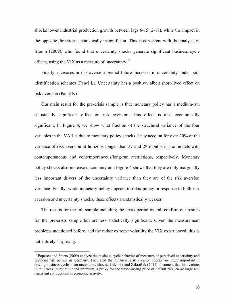
Our main result for the pre-crisis sample is that monetary policy has a medium-run

statistically significant effect on risk aversion. This effect is also economically

significant. In Figure 4, we show what fraction of the structural variance of the four

variables in the VAR is due to monetary policy shocks. They account for over 20% of the

variance of risk aversion at horizons longer than 37 and 29 months in the models with

contemporaneous and contemporaneous/long-run restrictions, respectively. Monetary

policy shocks also increase uncertainty and Figure 4 shows that they are only marginally

less important drivers of the uncertainty variance than they are of the risk aversion

variance. Finally, while monetary policy appears to relax policy in response to both risk

aversion and uncertainty shocks, these effects are statistically weaker.

The results for the full sample including the crisis period overall confirm our results

for the pre-crisis sample but are less statistically significant. Given the measurement

problems mentioned before, and the rather extreme volatility the VIX experienced, this is

not entirely surprising.

11 Popescu and Smets (2009) analyze the business cycle behavior of measures of perceived uncertainty and financial risk premia in Germany. They find that financial risk aversion shocks are more important in driving business cycles than uncertainty shocks. Gilchrist and Zakrajšek (2011) document that innovations to the excess corporate bond premium, a proxy for the time-varying price of default risk, cause large and persistent contractions in economic activity.

17

3.2 Robustness

In this subsection, we consider five types of robustness checks: 1) measurement of the

monetary policy stance; 2) measurement of the business cycle variable; 3) alternative

orderings of variables; 4) accounting for the sampling error in RA and UC estimates; and

5) conducting the analysis using a six variable monetary VAR with the Fed funds rate

and price level measures CPI and PPI entering as separate variables. We also verified that

our results remain robust to the use of both shorter and longer VAR lag-lengths. We

estimated a VAR with 1 lag, as selected by the Schwarz criterion, as well as a VAR with

4 lags (we did not go beyond four lags as otherwise the saturation ratio, the ratio of data

points to parameters, drops below 10). Our results were unaltered.

3.2.1 Measuring Monetary Policy

Table 2 reports summary statistics on the interaction of alternative measures of the

monetary policy stance with risk aversion (Panel A) and with uncertainty (Panel B). The

results confirm that a looser monetary policy stance lowers risk aversion in the short to

medium run. This effect is persistent, lasting for about two years. In some cases, the

immediate effect has the reverse sign however. In the other direction, monetary policy

becomes laxer in response to positive risk aversion shocks but the effect is statistically

significant in less than half the cases. As for the effect of monetary policy on uncertainty,

monetary tightening increases uncertainty in the medium run but this effect is not

significant when using the Fed fund rate. In the other direction, higher uncertainty leads

to laxer monetary policy in all specifications but the effect is only significant when using

the Fed fund rate under contemporaneous identifying restrictions.

3.2.2 Measuring Business Cycle Variation

18

We consider the log-difference of employment and the log of the ISM index as

alternative business cycle indicators. Unlike industrial production and employment, the

ISM index is a stationary variable, implying that VAR shocks do not have a long run

effect on it. Our long-run restriction on the effect of monetary policy is thus stronger

when applied to the ISM: it restricts the total effect of monetary policy on the ISM to be

zero. Nevertheless, our main results from Section 3.1 are confirmed for each specification

with an alternative business cycle variable. We present a full set of IRFs (the equivalent

of Figure 3) for the VARs with the log-difference of employment and the log of the ISM

index as business cycle measures in the Online Appendix (Figures OA4 and OA5,

respectively).

3.2.3 Alternative Orderings of Variables

In one alternative ordering, we reverse the order of risk aversion and uncertainty in

our benchmark VAR. In another robustness check, we order the real interest rate last,

thus allowing it to respond instantaneously to RA and UC shocks. We consistently find

that looser monetary policy lowers risk aversion and uncertainty in a statistically

significant fashion in the medium-run. In the other direction, the effects are less robust. In

the specification with RA and UC reversed, monetary policy mostly responds to UC

shocks, but the response to RA shocks is statistically insignificant. In the specification

with RERA ordered last, monetary policy responds to both positive RA and UC shocks

by loosening its stance, and the effect is statistically significantly different from zero. We

present a full set of IRFs for the reversed ordering of RA and UC and for the

specification with RERA ordered last in the Online Appendix (Figures OA6 and OA7,

respectively).

19

3.2.4 Sampling Error in RA and UC

We check that our VAR results are robust to accounting for the sampling error in the

RA and UC estimation. We draw 100 alternative RA and UC series from the distribution

of RA and UC estimates (as described in section 2.1), and feed those into our

bootstrapped VAR. We estimate 100 VAR replications per set of alternative RA and UC

series. We then construct the usual 90% confidence bounds. The results are very similar

to those obtained without taking uncertainty surrounding RA and UC estimates into

account, and are presented in the Online Appendix (Figure OA8).

3.2.5 Six-variable Monetary VAR

We also estimate a six-variable monetary VAR following Christiano, Eichenbaum

and Evans (1999) and featuring the nominal Fed funds rate as the measure of monetary

policy stance and price level measures CPI and PPI as additional variables.12 To identify

monetary policy shocks, we use a Cholesky ordering with CPI and industrial production

ordered first, followed by the Fed funds rate and PPI, and risk aversion and uncertainty

ordered last.

We present impulse-responses to monetary policy shocks in Figure 5. Again, we

discuss results for the pre-crisis sample, but summarize the full sample results in

parentheses. A positive monetary policy shock corresponds to a 15 basis points (30 in the

full sample) increase in the Fed funds rate. A contractionary monetary shock leads to a

statistically significant decrease in the CPI between lags 3 and 23 (2 and 8) and in the PPI

between lags 23 and 50 (effect insignificant in the full sample). Furthermore, in the pre-

crisis sample, industrial production declines following a monetary contraction after about

12 We estimate the model with four lags, as suggested by the Akaike criterion. All variables are in logarithms except for the Fed funds rate. Note that industrial production now enters the VAR in levels.

20

10 months, though the effect is not statistically significant (similarly, the effect is

insignificant in the full sample). Importantly, the reactions of both risk aversion and

uncertainty are remarkably similar to those uncovered in our benchmark four-variable

VARs. Looser monetary policy decreases risk aversion by 0.024 (0.023) after 12 (19)

months. The effect reaches a maximum of 0.040 (0.025) at lag 23 (24), and remains

statistically significant till lag 35 (till lag 37, significant under 68% confidence bounds).

The effects remain economically important as monetary policy shocks account for over

12% (3%) of the variance of risk aversion at horizons longer than 40 months (see Panel F

of Figure 5) but these percentages are nonetheless lower than in our four-variable VAR.

As for uncertainty, a higher Fed funds rate increases uncertainty between lags 12 and 31

(16 and 36), with the maximum impact of 0.040 (0.033) at lag 23 (22), which is also

consistent with our previous findings. In non-reported results, monetary policy responds

to both positive RA and UC shocks by loosening its stance. The effect is statistically

significant under 90% confidence bounds between lags 2 and 7 (6 and 15) for RA and

between lags 5 and 26 (3 and 20) for UC.

4. Alternative Identification of Monetary Policy Shocks

In this Section, we employ two alternative methodologies to identify monetary policy

shocks: 1) monetary surprises based on high-frequency Fed funds futures and 2) monthly

surprises calculated using daily Fed funds futures.

4.1 Identification using High-Frequency Fed Funds Futures

Our VAR set-up to identify monetary policy shocks and their structural relationship

with risk aversion and uncertainty follows the Sims (1980, 1998) identification tradition.

With financial market values changing continuously during the month, the use of

21

monthly data for this purpose certainly may cast some doubt on this identification

scheme. We therefore use an alternative identification methodology that makes use of

high frequency data to infer restrictions on the monthly VAR. The approach, inspired by

and building on the procedure described in D’Amico and Farka (2011), consists of three

steps.

In the first step, we measure the structural monetary policy and business cycle shocks

directly. For monetary policy, we rely on a well-established literature that uses high

frequency changes in Fed funds futures rates (see, for example, Faust, Swanson and

Wright, 2004) to measure monetary policy shocks, and we detailed their measurement in

Section 2. Likewise, for business cycle shocks, we use news announcements. Under

certain assumptions, these shocks can be viewed as measuring the structural shocks εt in

the VAR. For monetary policy shocks, this is plausible because usually only one shock

occurs per month, and the use of high frequency futures data helps ensure that the

identified shock is plausibly orthogonal to other shocks. As to the business cycle shocks,

there are a number of potentially important complicating issues, such as the correlation

between the different news announcements and the structural shock to the actual business

cycle variable used in the VAR, and the scale of the shocks when more than one occurs

within a particular month. However, these issues become moot when business cycle

shocks do not generate significant contemporaneous effects on our financial variables,

which ends up being the case.

In the second step, we measure the high frequency effects of monetary policy and

economic news surprises on risk aversion and uncertainty. We regress daily changes in

risk aversion and uncertainty (as proxies for unexpected changes to these variables),

22

respectively, on the monetary policy surprises based on high-frequency futures (using the

“tight” window shocks)13 and the four monthly economic news surprises concerning

industrial production (ΔIP), the ISM index (ΔISM), non-farm payroll and employment

(ΔEMP), as described in Section 2.3.14 The resulting coefficients for the pre-crisis sample

(with heteroskedasticity-robust standard errors in parentheses) are as follows:

ΔRAt = -0.039 + 0.047 ΔMPt – 0.005 ΔIPt – 0.004 ΔISMt – 0.004 ΔEMPt (7) (0.007) (0.020) (0.014) (0.016) (0.017)

ΔUCt = -0.009 + 0.013 ΔMPt + 0.002 ΔIPt – 0.002 ΔISMt – 0.008 ΔEMPt (8) (0.003) (0.010) (0.005) (0.005) (0.011)

The coefficients on the business cycle news surprises are not statistically different

from zero and economically small. However, the responses to the monetary policy

surprises are quantitatively larger and statistically significant at the 5% level for RA and

at the 16% level for UC. The coefficients on ΔMP give us direct evidence on the

contemporaneous responses of RA and UC to structural disturbances in MP. We already

note that these responses confirm that risk aversion reacts positively to monetary policy

shocks and does so more strongly than uncertainty. By the same token, we conclude that

the contemporaneous responses of RA and UC to a business cycle shock in our VARs are

equal to zero.

In the third step, we use the estimates of structural responses of RA and UC to

monetary policy and business cycle shocks in our VAR analysis. This requires a number

of additional assumptions. In particular, we assume that there are no further policy or

business cycle shocks during the month and thus that the monthly shock equals the daily

13 Results for the monetary policy surprises calculated using the “wide” window are very similar. 14 We treat both the non-farm payroll and the negative of the unemployment surprises as news about employment (ΔEMP) as they have similar information content. Whenever then come out on the same day (which is mostly the case), we sum them up.

23

shock identified from high frequency data. Furthermore, we assume that the

contemporaneous daily change in risk aversion and uncertainty identifies the monthly

change in unexpected risk aversion and uncertainty due to these policy and business cycle

shocks. In other words, we assume that the high-frequency regressions effectively yield

four coefficients in the A-1 matrix of our structural VAR. Because we need 6 restrictions

in total, we impose two more restrictions from a Cholesky ordering to achieve

identification. In one identification scheme (Model 1), we impose that both industrial

production and monetary policy do not instantaneously respond to RA; in another

scheme, we impose the same restrictions on the reaction to UC (Model 2).15 Because the

identifying assumptions on monetary policy shocks have more support in the extant

literature than the assumptions we made regarding the business cycle shocks, we also

consider a robustness check where we only impose the high-frequency responses to

monetary policy surprises in the monthly VAR. We then need four additional restrictions

from a Cholesky ordering to complete identification and use the three contemporaneous

restrictions in the BC equation (the usual assumption on sluggish adjustment of macro to

financial data) and a zero response by monetary policy to either RA (Model 3) or UC

(Model 4).

For the full sample, all the estimated coefficients in the second step regressions are

not statistically different from zero, but the effect of monetary policy shocks on risk

aversion is again positive with a t-stat of close to 1. If we were to impose that the

contemporaneous responses of RA and UC to monetary policy and business cycle shocks

are all equal to zero, models 1 and 2 would be under-identified. We thus estimate only

15 Imposing zero-response restrictions to RA and UC in the BC equation would lead to an under-identified model.

24

models 3 and 4 for the full sample, i.e., imposing the zero-response to monetary policy

surprises from the second step regression, plus three contemporaneous restrictions in the

BC equation and a zero response by monetary policy to either RA or UC. As before, we

report results for the full sample in parentheses (and present IRFs in the Online

Appendix, Figure OA2).

For the two models imposing four restrictions from the first step, we present impulse-

responses to monetary policy shocks in Figure 6. Looser monetary policy (corresponding

to a 29 basis points decrease in the real rate) lowers risk aversion on impact and between

lags 8 and 12, with a maximum impact of 0.055 in the model with no contemporaneous

response of business cycle and monetary policy to RA. The maximum impact is 0.061

and the effect is significant between lags 7 and 17 in the model with no contemporaneous

response of business cycle and monetary policy to UC.

As Panel B shows, a positive shock to the real rate increases uncertainty on impact in

the model with no contemporaneous response of the business cycle and monetary policy

to RA. The effect is positive but not statistically significant in the medium run. In the

model with no contemporaneous response of business cycle and monetary policy to UC,

the positive effect of the real rate shock on uncertainty is statistically significant on

impact and between lags 10-14, with a maximum impact of 0.059 at lag 14.

Lastly, the impact of monetary policy on industrial production growth is not

statistically significant (Panel C). Note that with different measures for the business

cycle, such as employment, the VAR does produce the expected and statistically

significant response to monetary policy.

25

For the two models imposing two restrictions (for the monetary policy shocks only)

from the first step, we present impulse-responses to monetary policy shocks in Figure 7.

Looser monetary policy, corresponding to a 33 (42) basis points decrease in the real rate,

lowers risk aversion on impact and between lags 4-36 (14-37, significant at 68%

confidence bounds), with a maximum impact of 0.055 at lag 15 (0.023 at lag 17) both in

the model with no contemporaneous response of monetary policy to RA and in the model

with no contemporaneous response of monetary policy to UC (and the three zero

restrictions in the BC equation).

As Panel B shows, a positive shock to the real rate increases uncertainty on impact

and between lags 4-36, with a maximum impact of 0.058 at lag 16 both in the model with

no contemporaneous response of monetary policy to RA and in the model with no

contemporaneous response of monetary policy to UC (and the three zero restrictions in

the BC equation). (The impact of the monetary policy shock on uncertainty is positive but

not statistically significant at 68% confidence bounds for the full sample.)

Lastly, the impact of monetary policy on industrial production growth is again not

statistically significant (Panel C).

4.2 Identification using Daily Fed Funds Futures

In this section, we adopt the approach of Bernanke and Kuttner (2005) to study the

dynamic response of risk aversion and uncertainty to monetary policy. The key feature of

their approach is the calculation of a monthly monetary policy surprise using Federal

funds futures contracts. This variable identifies the monetary policy shock and is included

in the VAR as an exogenous variable. The endogenous variables in the VAR are RA, UC

and the log difference of industrial production (DIPI).

26

We present impulse-responses to “cleansed” monetary policy shocks16 in Figure 7 for

the pre-crisis sample and in the Online Appendix for the full sample (Figure OA3). As

before, below we discuss results for the full sample in parentheses. The results generally

confirm that monetary policy surprises have a positive impact on both RA and UC, and

have the expected negative effect on industrial production. However, the results are less

strong statistically than under our other identification schemes.

A one standard deviation negative shock to the “cleansed” surprise, equivalent to 8.6

basis points (9 basis points), decreases RA on impact by 0.061 and UC by 0.054

(decreases RA by 0.053 and UC by 0.026). The IRFs are significant on impact at the 80%

confidence level for RA and at the 70% level for UC (at the 80% level for RA; not

statistically significant for UC). These results are robust to the use of alternative business

cycle indicators (non-farm employment and the ISM index).

5. Conclusions

A number of recent studies point at a potential link between loose monetary policy

and excessive risk-taking in financial markets. Rajan (2006) conjectures that in times of

ample liquidity supplied by the central bank, investment managers have a tendency to

engage in risky, correlated investments. To earn excess returns in a low interest rate

environment, their investment strategies may entail risky, tail-risk sensitive and illiquid

securities (“search for yield”). Moreover, a tendency for herding behavior emerges due to

the particular structure of managerial compensation contracts. Managers are evaluated

vis-à-vis their peers and by pursuing strategies similar to others, they can ensure that they

do not under perform. This “behavioral” channel of monetary policy transmission can

16 The monetary policy surprise is standardized by subtracting the mean and dividing by the standard deviation.

27

lead to the formation of asset prices bubbles and can threaten financial stability. Yet,

there is no empirical evidence on the links between risk aversion in financial markets and

monetary policy.

This article has attempted to provide a first characterization of the dynamic links

between risk, uncertainty and monetary policy, using a simple vector-autoregressive

framework. We decompose implied volatility into two components, risk aversion and

uncertainty, and study the interactions between each of the components and monetary

policy under a variety of identification schemes for monetary policy shocks. We

consistently find that lax monetary policy increases risk appetite (decreases risk aversion)

in the future, with the effect lasting for more than two years and starting to be significant

after nine months. The effect on uncertainty is similar but the immediate response of

uncertainty to monetary policy shocks in high frequency regressions is weaker than that

of risk aversion. Conversely, high uncertainty and high risk aversion lead to laxer

monetary policy in the near-term future but these effects are not always statistically

significant. These results are robust to controlling for business cycle movements.

Consequently, our VAR analysis provides a clean interpretation of the stylized facts

regarding the dynamic relations between the VIX and the monetary policy stance

depicted in Figure 1. The primary component driving the co-movement between past

monetary policy stance and current VIX levels (first column of Figure 1) is risk aversion

but uncertainty also reacts to monetary policy. Both components of the VIX lie behind

the negative relation in the opposite direction (second column of Figure 1).

We hope that our analysis will inspire further empirical work and research on the

exact theoretical links between monetary policy and risk-taking behavior in asset

28

markets. A recent literature, mostly focusing on the origins of the financial crisis, has

considered a few channels that deserve further scrutiny. Adrian and Shin (2008) stress the

balance sheets of financial intermediaries and repo growth; Adalid and Detken (2007)

and Alessi and Detken (2008) stress the buildup of liquidity through money growth and

Borio and Lowe (2002) emphasize rapid credit expansion.17 Recent work in the

consumption-based asset pricing literature attempts to understand the structural sources

of the VIX dynamics (see Bekaert and Engstrom (2010), Bollerslev, Tauchen and Zhou

(2009), Drechsler and Yaron (2011)). Yet, none of these models incorporates monetary

policy equations. In macroeconomics, a number of articles have embedded term structure

dynamics into the standard New-Keynesian workhorse model (Bekaert, Cho, Moreno

(2010), Rudebusch and Wu (2008)), but no models accommodate the dynamic

interactions between monetary policy, risk aversion and uncertainty, uncovered in this

article.

The policy implications of our work are potentially very important. Because monetary

policy significantly affects risk aversion and uncertainty and these financial variables

may affect the business cycle, we seem to have uncovered a monetary policy

transmission mechanism missing in extant macroeconomic models. Fed chairman

Bernanke (see Bernanke (2002)) interprets his work on the effect of monetary policy on

the stock market (Bernanke and Kuttner (2005)) as suggesting that monetary policy

would not have a sufficiently strong effect on asset markets to pop a “bubble” (see also

Bernanke and Gertler (2001), Gilchrist and Leahy (2002), and Greenspan (2002)).

17 In fact, we considered the effects of repo, money and credit growth on our results by including them in a four-variable VAR together with RA, UC, and RERA (replacing the BC variable). We consistently found that the direct effect of monetary policy on risk aversion and uncertainty we uncovered in our benchmark VARs is preserved.

29

However, if monetary policy significantly affects risk appetite in asset markets, this

conclusion may not hold. If one channel is that lax monetary policy induces excess

leverage as in Adrian and Shin (2008), perhaps monetary policy is potent enough to weed

out financial excess. Conversely, in times of crisis and heightened risk aversion,

monetary policy can influence risk aversion and uncertainty in the market place, and

therefore affect real outcomes.

Acknowledgements

We thank Tobias Adrian, Gianni Amisano, David DeJong, Bartosz Mackowiak,

Frank Smets, José Valentim and Jonathan Wright for helpful comments and suggestions.

Falk Bräuning and Carlos Garcia de Andoain Hidalgo provided excellent research

assistance. The views expressed do not necessarily reflect those of the European Central

Bank or the Eurosystem.

30

REFERENCES

Adalid, R. and C. Detken (2007). “Liquidity Shocks and Asset Price Boom/Bust Cycles,” ECB Working Paper No. 732.

Adrian, T. and H. S. Shin (2008). “Liquidity, Monetary Policy, and Financial Cycles,” Current Issues in Economics and Finance 14 (1), Federal Reserve Bank of New York.

Alessi, L. and C. Detken (2009). “Real-time Early Warning Indicators for Costly Asset Price Boom/Bust Cycles - A Role for Global Liquidity,” ECB Working Paper No. 1039.

Altunbas, Y., L. Gambacorta and D. Marquéz-Ibañez (2010). “Does Monetary Policy Affect Bank Risk-taking?”, ECB Working Paper No. 1166.

Baker, M. and J. Wurgler (2007). “Investor Sentiment in the Stock Market,” Journal of Economic Perspectives 21, pp. 129-151.

Bakshi, G. and D. Madan (2000). “Spanning and Derivative-Security Valuation,” Journal of Financial Economics 55 (2), pp. 205-238.

Bakshi, G., N. Kapadia and D. Madan (2003). “Stock Return Characteristics, Skew Laws, and Differential Pricing of Individual Equity Options,” Review of Financial Studies 16 (1), pp. 101-143.

Bekaert, G., S. Cho and A. Moreno (2010). “New Keynesian Macroeconomics and the Term Structure,” Journal of Money, Credit and Banking 42 (1), pp. 33-62.

Bekaert, G. and E. Engstrom (2010). “Asset Return Dynamics under Bad Environment-Good Environment Fundamentals,” working paper, Columbia GSB.

Bekaert, G., E. Engstrom, and Y. Xing (2009). “Risk, Uncertainty, and Asset Prices,” Journal of Financial Economics 91, pp. 59-82.

Bernanke, B. (2002). “Asset-Price ‘Bubbles’ and Monetary Policy,” speech before the New York chapter of the National Association for Business Economics, New York, New York, October 15.

Bernanke, B. and M. Gertler (2001). “Should Central Banks Respond to Movements in Asset Prices?” American Economic Review 91 (May), pp. 253-57.

Bernanke, B. and K. N. Kuttner (2005). “What Explains the Stock Market’s Reaction to Federal Reserve Policy?” Journal of Finance 60 (3), pp. 1221-1257.

Bernanke, B. and I. Mihov (1998a). “Measuring Monetary Policy,” Quarterly Journal of Economics 113 (3), pp. 869-902.

Bernanke, B. and I. Mihov (1998b). “The Liquidity Effect and Long-run Neutrality,” Carnegie-Rochester Conference Series on Public Policy 49 (1), pp. 149-194.

Blanchard, O. (2009). “Nothing to Fear but Fear Itself,” Economist, January 29.

31

Blanchard, O. and D. Quah (1989). “The Dynamic Effects of Aggregate Demand and Supply Disturbances,” American Economic Review 79 (4), pp. 655-73.

Bloom, N. (2009). “The Impact of Uncertainty Shocks,” Econometrica 77 (3), pp. 623-685.

Bloom, N., M. Floetotto and N. Jaimovich (2009). “Real Uncertain Business Cycles,” working paper, Stanford University.

Bollerslev, T., G. Tauchen and H. Zhou (2009). “Expected Stock Returns and Variance Risk Premia,” Review of Financial Studies 22 (11), pp. 4463-4492.

Borio, C. and P. Lowe (2002). “Asset Prices, Financial and Monetary Stability: Exploring the Nexus,” BIS Working Paper No. 114.

Borio, C. and H. Zhu (2008). “Capital Regulation, Risk-Taking and Monetary Policy: A Missing Link in the Transmission Mechanism?” BIS Working Paper No. 268.

Breeden, D. and R. Litzenberger (1978). “Prices of State-contingent Claims Implicit in Option Prices,” Journal of Business 51 (4), pp. 621-651.

Britten-Jones, M. and A. Neuberger (2000). “Option Prices, Implied Price Processes, and Stochastic Volatility,” Journal of Finance 55, pp. 839-866.

Campbell, J. Y and J. Cochrane (1999). “By Force of Habit: A Consumption Based Explanation of Aggregate Stock Market Behavior,” Journal of Political Economy 107 (2), pp. 205-251.

Carr, P. and L. Wu (2009). “Variance Risk Premiums,” Review of Financial Studies 22 (3), pp. 1311-1341.

Chicago Board Options Exchange (2004). “VIX CBOE Volatility Index,” White Paper.

Christiano, L. J., M. Eichenbaum and C. L. Evans (1996). “The Effects of Monetary Policy Shocks: Evidence from the Flow of Funds,” The Review of Economics and Statistics 78(1), pp. 16-34.

Christiano, L. J., M. Eichenbaum and C. L. Evans (1999). “Monetary Policy Shocks: What Have We Learned and to What End?” In J. B. Taylor and M. Woodford (eds.), Handbook of Macroeconomics, Vol. 1A, pp. 65-148, North-Holland.

Coudert, V. and M. Gex (2008). “Does Risk Aversion Drive Financial Crises? Testing the Predictive Power of Empirical Indicators,” Journal of Empirical Finance 15, pp. 167-184.

D’Amico and Farka (2011). “The Fed and the Stock Market: An Identification Based on Intraday Futures Data,” Journal of Business and Economic Statistics 29(1), pp. 126-137.

32

Drechsler, I. (2009). “Uncertainty, Time-Varying Fear, and Asset Prices,” working paper, Wharton School.

Drechsler, I. and A. Yaron (2011). “What’s Vol Got to Do with It,” Review of Financial Studies 24(1), pp. 1-45.

Ehrmann, M. and M. Fratzscher (2004). “Exchange Rates and Fundamentals: New Evidence from Real-time Data,” ECB Working Paper No. 365.

Faust, J., E. Swanson, and J. Wright (2004). “Identifying VARs Based on High Frequency Futures Data,” Journal of Monetary Economics 51(6), pp. 1107-1131.

Gilchrist, S. and J.V. Leahy (2002). “Monetary Policy and Asset Prices,” Journal of Monetary Economics 49 (1), pp. 75-97.

Gilchrist, S. and E. Zakrajšek (2012). “Credit Spreads and Business Cycle Fluctuations,” American Economic Review 102(4), pp. 1692–1720.

Greenspan, A. (2002). “Economic Volatility,” speech before a symposium sponsored by the Federal Reserve Bank of Kansas City, Jackson Hole, Wyoming, August 30.

Gürkaynak, R. S., B. Sack and E. T. Swanson (2005). “Do Actions Speak Louder Than Words? The Response of Asset Prices to Monetary Policy Actions and Statements,” International Journal of Central Banking 1 (1), pp. 55-92.

Ioannidou, V. P., S. Ongena and J.-L. Peydró (2009). “Monetary Policy, Risk-Taking and Pricing: Evidence from a Quasi Natural Experiment,” European Banking Center Discussion Paper No. 2009-04S.

Jiménez, G., S. Ongena, J.-L. Peydró and J. Saurina (2009). “Hazardous Times for Monetary Policy: What do Twenty-Three Million Bank Loans Say About the Effects of Monetary Policy on Credit Risk?”, CEPR Discussion Paper No. 6514.

Johansen, S. (1995). Likelihood-Based Inference in Cointegrated Vector Auto-Regressive Models. Oxford: Oxford University Press.

King, R. and M. W. Watson (1992). “Testing Long Run Neutrality,” NBER Working Papers No. 4156, National Bureau of Economic Research.

Kuttner, K. N. (2001). “Monetary Policy Surprises and Interest Rates: Evidence from the Fed Funds Futures Market,” Journal of Monetary Economics 47 (3), pp. 523-544.

Maddaloni, A. and J.-L. Peydró (2010). “Bank Risk-Taking, Securitization, Supervision, and Low Interest Rates: Evidence from Lending Standards,” forthcoming in the Review of Financial Studies.

Newey, W. and K. West (1987). “A Simple, Positive Semi-definite, Heteroskedasticity and Autocorrelation Consistent Covariance Matrix,” Econometrica 55(3), pp. 703-708.

33

Popescu, A. and F. Smets (2009). “Uncertainty, Risk-taking and the Business Cycle in Germany,” CESifo Economic Studies 56(4), pp. 596-626. Rajan, R. (2006). “Has Finance Made the World Riskier?” European Financial Management 12 (4), pp. 499-533.

Rigobon, R. and B. Sack (2003). “Measuring the Reaction of Monetary Policy to the Stock Market,” Quarterly Journal of Economics 118 (2), pp. 639-669.

Rigobon, R. and B. Sack (2004). “The Impact of Monetary Policy on Asset Prices,” Journal of Monetary Economics 51 (8), pp. 1553-1575.

Rubio-Ramírez, J. F., D. F. Waggoner and T. Zha (2010). “Structural Vector Autoregressions: Theory of Identification and Algorithms for Inference,” Review of Economic Studies 77(2), pp 665-696.

Rudebusch, G. D (2009). “The Fed’s Monetary Policy Response to the Current Crisis,” The Federal Reserve Bank of San Francisco Economic Letter, May 2009.

Rudebusch, G. D. and T. Wu (2008). “A Macro-Finance Model of the Term Structure, Monetary Policy and the Economy,” Economic Journal 118 (530), pp. 906-926.

Sims, C.A. (1980). “Macroeconomics and Reality,” Econometrica 48(1), pp. 1-48.

Sims, C.A. and T. Zha (1998). “Comment on Glenn Rudebusch’s “Do measures of monetary policy in a VAR make sense," International Economic Review 39(4), pp. 933-941.

Sims, C.A. and T. Zha (1999). “Error Bands for Impulse Responses," Econometrica 67(5), pp. 1113-1155.

Taylor, J. B. (1993). “Discretion Versus Policy Rules in Practice,” Carnegie-Rochester Conference Series on Public Policy 39, pp. 195–214.

Thorbecke, W. (1997). “On Stock Market Returns and Monetary Policy,” Journal of Finance 52 (2), pp. 635-654.

Whaley, R. E. (2000). “The Investor Fear Gauge,” Journal of Portfolio Management, Spring, pp. 12-17.

Wright, J. H. (2011). “What does Monetary Policy do to Long-Term Interest Rates at the Zero Lower Bound?” working paper, Johns Hopkins University.

34

Figure 1: Cross-correlogram LVIX RERA

Notes: The first column presents the (lagged) cross-correlogram between the log of the VIX (LVIX) and past values of the real interest rate (RERA). The second column presents the (lead) cross-correlogram between LVIX and future values of RERA. Dashed vertical lines indicate 95% confidence intervals for the cross-correlation. The third column presents the cross-correlation values. The index i indicates the number of months either lagged or led for the real interest rate variable.

35

Table 1: Description of variables

Name Label Description (source)

Consumer price index CPI Consumer price index, all items

Dividend yield Dividend yield of the Standard & Poor 500 index

Fed funds rate FED Fed funds target rate

Implied volatility LVIX Implied volatility of options on the Standard & Poor 500 index, Log (VIX / 12 )

(Growth of) Industrial production (D)IPI Log (difference of) total industrial production index

ISM index ISM ISM Purchasing Managers index

M1 money aggregate growth M1 Month-on-month growth of M1

(Growth of) Non-farm employment (D)EMP Log (difference of) non-farm employment

Producer price index PPI Producer price index for intermediate materials

Real interest rate RERA FED minus annual CPI inflation rate

Realized variance RVAR Realized variance [see Section 2.1]

Risk aversion RA Log (risk aversion) [see Section 2.1]

Taylor Rule deviations TRULE FED minus Taylor rule rate [see Section 2.2]

Three-month T-bill Secondary market yield

Uncertainty (conditional variance) UC Log (uncertainty) [see Section 2.1]

Notes: Monthly frequency, end-of-the-month data (seasonally adjusted where applicable). Unless otherwise mentioned, the data are from Thomson Datastream.

36

Figure 2: Risk aversion and uncertainty

Panel A: Risk aversion

0

20

40

60

80

100

120

19

90

m1

19

91

m1

19

92

m1

19

93

m1

19

94

m1

19

95

m1

19

96

m1

19

97

m1

19

98

m1

19

99

m1

20

00

m1

20

01

m1

20

02

m1

20

03

m1

20

04

m1

20

05

m1

20

06

m1

20

07

m1

20

08

m1

20

09

m1

20

10

m1

Gulf War I

Mexican

Crisis

Asian

Crisis

Russian / LTCM

Crisis

Corporate

Scandals

High Risk

Appetite

Lehman

Aftermath

Euro Area

Debt Crisis

09/11

Panel B: Uncertainty

0

20

40

60

80

100

120

140

160

180

19

90

m1

19

91

m1

19

92

m1

19

93

m1

19

94

m1

19

95

m1

19

96

m1

19

97

m1

19

98

m1

19

99

m1

20

00

m1

20

01

m1

20

02

m1

20

03

m1

20

04

m1

20

05

m1

20

06

m1

20

07

m1

20

08

m1

20

09

m1

20

10

m1

Gulf War I

Mexican

Crisis

Asian

Crisis

Russian / LTCM

CrisisCorporate

Scandals

Low

Uncertainty

Lehman

Aftermath

Euro Area

Debt

Crisis09/11

Notes: Plots of risk aversion and uncertainty for our sample period (January 1990 – August 2010).

37

Figure 3: Structural-form IRFs for the 4-variable VAR (DIPI, RERA, RA, UC)

Panel A: Impulse RERA, response RA Contemporaneous restrictions Contemporaneous/long-run restrictions

Panel B: Impulse RA, response RERA

Contemporaneous restrictions Contemporaneous/long-run restrictions

Panel C: Impulse RERA, response UC


Panel D: Impulse UC, response RERA


38

Panel E: Impulse RERA, response DIPI Contemporaneous restrictions Contemporaneous/long-run restrictions

Panel F: Impulse DIPI, response RERA


Panel G: Impulse RA, response DIPI


Panel H: Impulse DIPI, response RA


39

Panel I: Impulse UC, response DIPI Contemporaneous restrictions Contemporaneous/long-run restrictions

Panel J: Impulse DIPI, response UC


Panel K: Impulse RA, response UC


Panel L: Impulse UC, response RA


Notes: Estimated structural impulse-response functions (black lines) and 90% bootstrapped confidence intervals (grey dashed lines) for the model with 3 lags (selected by Akaike), based on 1000 replications. Panels on the left present results of the model with contemporaneous (Cholesky) restrictions, panels on the right present results of the model with contemporaneous/long-run restrictions.

40

Figure 4: Structural variance decompositions

Impact of RERA shocks


Notes: Fractions of the structural variance due to RERA shocks for the four variables DIPI, RERA, RA and UC (model with 3 lags, selected by Akaike). The panel on the left presents results of the model with contemporaneous restrictions, the panel on the right presents results of the model with contemporaneous/long-run restrictions.

41

Table 2: Robustness to monetary policy measures

Panel A: Monetary policy instrument – risk aversion pair

MP instrument Impulse MP, response RA Impulse RA, response MP

sign significant from-to (month) sign significant from-to (month) Real interest rate

- COR - CLR

/+

/+

0 - 2 (), 9 - 40 (+) 2 (), 9 – 40 (+)

-- 12 - 24

Taylor rule - COR - CLR

/+

+

0 (), 8 - 44 (+) 9 – 44

-- --

Fed funds rate - COR - CLR

+

+

21 - 38 19 - 38

0 - 10 0 - 7

(-1) M1 growth - COR - CLR

/+

/+

-- --

-- --

(-1) M1 - COR

+

5 - 26

--

Panel B: Monetary policy instrument – uncertainty pair

MP instrument Impulse MP, response UC Impulse UC, response MP sign significant from-to (month) sign significant from-to (month)

Real interest rate - COR - CLR

/+ +

0 - 1 (), 11 - 38 (+) 0 - 3 (), 11 - 40 (+)

-- --

Taylor rule - COR - CLR

/+ /+

0 - 1 (), 15 - 42 (+) 0 - 1 (), 17 - 43 (+)

-- --

Fed funds rate - COR - CLR

/+ /+

-- --

14 - 31

-- (-1) M1 growth

- COR - CLR

+ +

3 - 12 3 - 12

-- --

(-1) M1 - COR

+

5 - 19

--

Notes: Table 4 summarizes results for the interactions between monetary policy (as represented by four different measures) and risk aversion (RA) in Panel A and between monetary policy and uncertainty (UC) in panel B in the four-variable model with DIPI, MP, RA and UC. The MP measures considered are: real rate, Taylor rule deviations, Fed funds rate, the negative of the M1 growth. Each Panel lists the range of months for which impulse-response functions (VARs with contemporaneous (COR) and contemporaneous/long-run (CLR) restrictions, respectively) were statistically significant within the 90% confidence interval in the direction indicated in the column “sign”. The last row in each panel considers a specification with M1 and industrial production both entering in levels rather than growth rates (COR restrictions only).

42

Figure 5: Monetary policy shock in the 6-variable VAR (CPI EMP FED PPI RA UC)

Panel A: Impulse FED, response CPI Panel B: Impulse FED, response PPI

Panel C: Impulse FED, response RA Panel D: Impulse FED, response UC

Panel E: Impulse FED, response IPI Panel F: Structural Variance Decompositions

Notes: Panels A-E: Estimated structural impulse-responses (black lines) to a monetary policy shock in the 6-variable model and 90% bootstrapped confidence intervals (dashed grey lines), for the model with 4 lags (selected by Akaike), based on 1000 replications. Panel F: Fractions of the structural variance due to FED shocks for the six variables.

43

Figure 6: Identification using high-frequency futures and business cycle news

announcements

Panel A: Impulse MP, response RA Model 1 Model 2

Panel B: Impulse MP, response UC

Model 1 Model 2

Panel C: Impulse MP, response DIPI

Model 1 Model 2

Notes: Estimated structural impulse-response functions (black lines) and 90% bootstrapped confidence intervals (grey dashed lines) for the model with 3 lags (selected by), based on 1000 replications. Four restrictions are derived from high frequency data. Panels on the left present results of Model 1 (BC and MP do not respond instantaneously to RA), panels on the right present results of Model 2 (BC and MP do not respond instantaneously to UC).

44

Figure 7: Identification using high-frequency futures

Panel A: Impulse MP, response RA Model 3 Model 4

Panel B: Impulse MP, response UC

Model 3 Model 4


Model 3 Model 4

Notes: Estimated structural impulse-response functions (black lines) and 90% bootstrapped confidence intervals (grey dashed lines) for the model with 3 lags (selected by), based on 1000 replications. Panels on the left present results of Model 3, panels on the right present results of Model 4. Both models assume zero contemporaneous responses of the BC shocks to the other variables. Model 3 (Model 4) assumes that monetary policy does not instantaneously react to RA (UC).

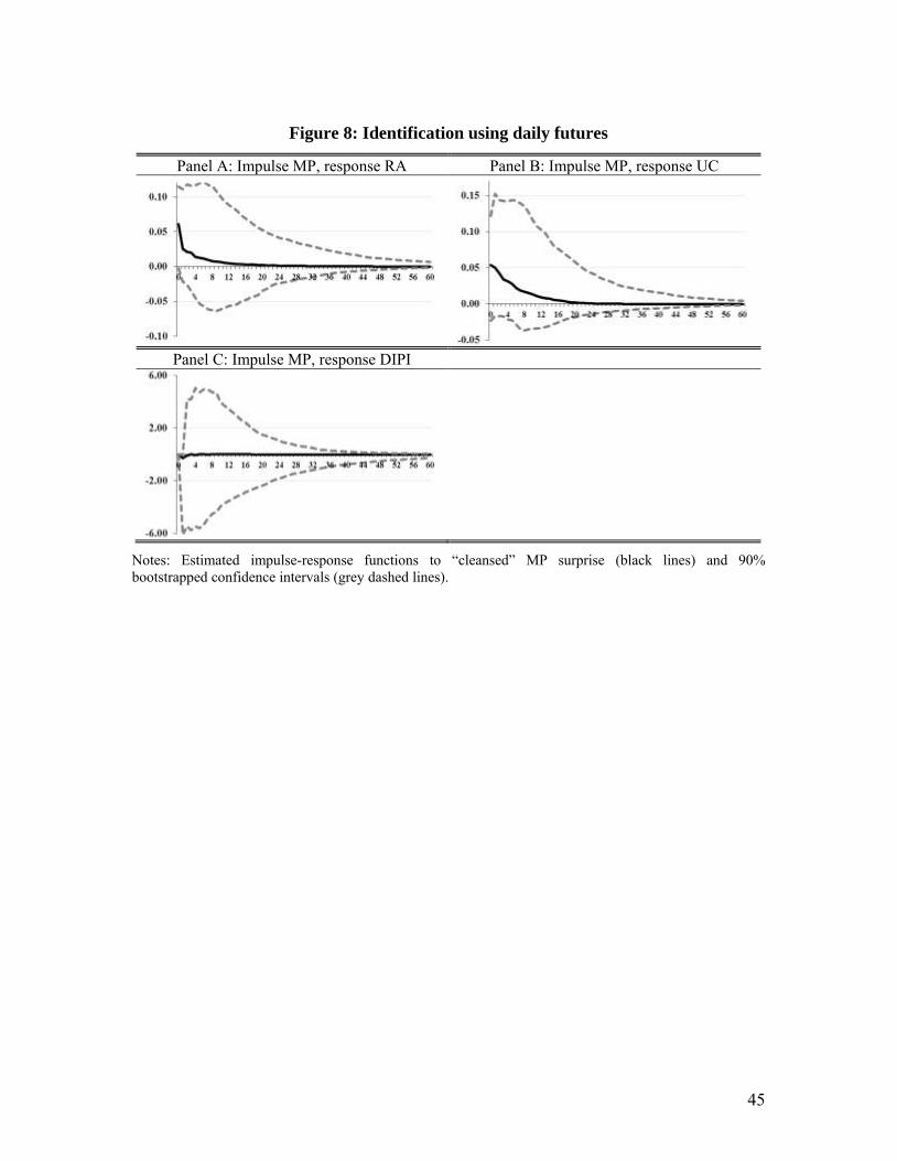
45

Figure 8: Identification using daily futures

Panel A: Impulse MP, response RA Panel B: Impulse MP, response UC


Notes: Estimated impulse-response functions to “cleansed” MP surprise (black lines) and 90% bootstrapped confidence intervals (grey dashed lines).

46

Appendix: The VIX and Risk

To obtain intuition on how the VIX is related to the actual (“physical”) expected

variance of stock returns and to risk preferences, we analyze a one-period discrete state

economy. Imagine a stock return distribution with three different states ix , as follows:

Good state: axg with probability 2/)1( p ,

Bad state : axb with probability 2/)1( p ,

Crash state: cxc with probability p ,

where 0 , 0a and 0p are parameters to be determined. We set them to match

moments of US stock returns - the mean, the variance (standard deviation) and the

skewness - while fixing the crash return at an empirically plausible number.

The mean is given by:

pcppcxp

xp

X bg

)1(2

12

1 . (1)

The variance is given by:

2222 )()(2

1)(2

1XcpXa

pXa

pV

(2)

and the skewness ( Sk ) by:

33323

)()(2

1)(2

1XcpXa

pXa

pSkV

. (3)

Consider an investor with power utility over wealth in a one-period world, so that in

equilibrium she invests her entire wealth in the stock market:

1)~(

)~(1

0 RWEWU , (4)

where R~ is the gross return on the stock market, 0W is initial wealth and is the

coefficient of relative risk aversion.

The “pricing kernel” in this economy is given by marginal utility, denoted by m , and

is proportional to R~ . Hence, the stochastic part of the pricing kernel moves inversely

with the return on the stock market. When the stock market is down, marginal utility is

relatively high and vice versa.

47

The physical variance of the stock market is exogenous in this economy, and is

simply given byV . This variance is computed using the actual probabilities. The VIX

represents the “risk-neutral” conditional variance. It is computed using the so-called

“risk-neutral probabilities,” which are simply probabilities adjusted for risk.

In particular, for a general state probability i for state i , the risk-neutral probability

is:

mE

R

mE

m i

i

i

i

RN

i

. (5)

So, for a given , we can easily compute the risk-neutral probabilities since 1 ii xR .

For an economy with K states, the risk-neutral variance is then given by:

2

1

2 )( XxVIX i

K

i

RN

i

(6)

and the variance premium is:

2

1

2 )()( XxVVIXVP i

K

i

i

RN

i

. (7)

In our economy, the risk-neutral probability puts more weight on the crash state and

the crash state induces plenty of additional variance, rendering the variance premium

positive. The higher is risk aversion, the more weight the crash state gets, and the higher

the variance premium will be. The expression for the variance premium has a particularly

simple form:

222 ))(())(2

1())(2

1( XxpXxp

Xxp

VP c

RN

cb

RN

bg

RN

g

(8)

where mE

apRN

g

)1(2

1 , mE

apRN

b

)1(2

1 and mE

cpRN

c

)1( .

Numerical Examples

Suppose the statistics to match are as follows: %10X , %15 , both on an

annualized basis; and 1Sk on a monthly basis. We set %25c (a monthly number).

This crash return is in line with the stock market collapses in October 1987 and October

2008. The implied crash probability to match the skewness coefficient of -1 is given

by % 5.0p . With a monthly investment horizon, the crash probability implies a crash

every 200 months, or roughly once every two decades. Panel A of Appendix Table 1

48

provides, for different values of the coefficient of relative risk aversion , the values for

the VIX on an annualized basis in percent (VIX), the log of the VIX on a monthly basis

(LVIX), i.e., log(VIX 12/ ), the annualized variance premium (VP), and our risk

aversion proxy computed on a monthly basis (RA), i.e., log(VIX 12/12/ 22 ). Note

that the variance premium and our risk aversion measure are monotonically increasing in

the coefficient of relative risk aversion .

In structural models, is typically assumed to be time-invariant, and the time

variation in the variance premium is generated through different mechanisms. For

example, in Drechsler and Yaron (2011), who formulate a consumption-based asset

pricing model with recursive preferences, the variance premium is directly linked to the

probability of a “negative jump” to expected consumption growth. The analogous

mechanism in our simple economy would be to decrease the skewness of the return

distribution by increasing the crash probability p . This obviously represents “risk”

instead of “risk aversion”. Yet, it is the interaction of risk aversion and skewness that

gives rise to large readings in our risk aversion proxy. To illustrate, let us consider an

example with lower skewness. Setting skewness equal to -2 requires a higher crash

probability of % 1p . Panel B of Appendix Table 1 shows that the VIX increases, and

increases more the higher the coefficient of relative risk aversion, both in absolute and in

relative terms. The variance premium roughly doubles for all levels, whereas our risk

aversion proxy increases by about 0.7.

In Bekaert and Engstrom (2010), when a recession becomes more likely, the

representative agent also becomes more risk averse through a Campbell-Cochrane

(1999)-like external habit formulation. The recession fear then induces high levels of the

VIX. We can informally illustrate such a mechanism in our one-period model. Imagine

that the utility function is over wealth relative to an exogenous benchmark wealth level

bmW . Normalizing the initial wealth 0W to 1, the pricing kernel is now given by

bmWR

~ , and the coefficient of relative risk aversion is bmWRR ~/~

. Consequently,

risk aversion is state dependent and increases as R~ decreases towards the benchmark

level. It is easy to see how a dynamic version of this economy, for instance with a slow-

49

moving bmW , could generate risk aversion that is changing over time as return

realizations change the distance between actual wealth and the benchmark wealth level.

To illustrate this mechanism, Panel C considers three different benchmark levels for

bmW (0.05, 0.25 and 0.5) with fixed at 4 and 1Sk , implying % 5.0p . The

second column shows expected relative risk aversion in the economy (CRRA), weighting

the three possible realizations for risk aversion with the actual state probabilities. The

other columns are as in the panels above. Clearly, for 0bmW , CRRA = 4 and we

replicate the values in Panel A for 4 . Keeping fixed and increasing bmW , effective

risk aversion increases. For example, CRRA increases from 4.21 to 7.97 as bmW increases

from 0.05 to 0.5. The VIX increases from 17.87 to 27.93 and our risk aversion proxy RA

increases from 2.06 to 3.83. In sum, our risk aversion measure monotonically increases

with true risk aversion in the underlying economy.

Appendix Table 1: The VIX and Risk Aversion

Panel A: Varying , 1Sk , % 5.0p Parameters VIX LVIX VP RA

2,1 Sk 15.987 1.529 0.003 0.936 4,1 Sk 17.612 1.626 0.008 1.960 6,1 Sk 20.139 1.760 0.018 2.711

Panel B: Varying , 2Sk , % 1p Parameters VIX LVIX VP RA

2,2 Sk 16.908 1.585 0.006 1.624 4,2 Sk 19.841 1.745 0.017 2.643 6,2 Sk 24.075 1.939 0.036 3.386

Panel C: Varying bmW , 4 , 1Sk , % 5.0p

Parameters CRRA VIX LVIX VP RA 0,4 bmW 4.000 17.612 1.626 0.008 1.960

05.0,4 bmW 4.209 17.868 1.641 0.009 2.061 25.0,4 bmW 5.323 19.598 1.733 0.016 2.584 50.0,4 bmW 7.968 27.934 2.087 0.056 3.835

Notes: Values of the VIX on an annualized basis in percent (VIX), the log of the VIX on a monthly basis (LVIX), the annualized variance premium (VP), and our proxy for risk aversion on a monthly basis (RA) for different values of the underlying parameters, while keeping the crash return c fixed at -25%. In Panel A, the varying parameter is the coefficient of relative risk aversion γ while skewness Sk is fixed at -1. In Panel B, skewness Sk is fixed at -2. Panel C computes, for γ fixed at 4 and Sk fixed at -1, expected risk aversion (CRRA) and the other four variables for different values of the benchmark wealth level Wbm.

RISK, UNCERTAINTY AND MONETARY POLICY … · Risk, Uncertainty and Monetary Policy Geert Bekaert,...

Documents

Transcript of RISK, UNCERTAINTY AND MONETARY POLICY … · Risk, Uncertainty and Monetary Policy Geert Bekaert,...