
Risk Sharing and Transactions Costs: Evidence from Kenya’s Mobile Money … · Risk Sharing and...
41
American Economic Review 2014, 104(1): 183–223 http://dx.doi.org/10.1257/aer.104.1.183 183 Risk Sharing and Transactions Costs: Evidence from Kenya’s Mobile Money Revolution † By William Jack and Tavneet Suri* We explore the impact of reduced transaction costs on risk sharing by estimating the effects of a mobile money innovation on consumption. In our panel sample, adoption of the innovation increased from 43 to 70 percent. We find that, while shocks reduce consumption by 7 percent for nonusers, the consumption of user households is unaffected. The mechanisms underlying these consumption effects are increases in remittances received and the diversity of senders. We report robustness checks supporting these results and use the four-fold expansion of the mobile money agent network as a source of exogenous variation in access to the innovation. (JEL E42, G22, O16, O17, Z13) In developing countries, informal networks provide an important means by which individuals and households share risk, though the insurance they provide is often incom- plete. Economists have proposed a number of reasons for this incompleteness, includ- ing information asymmetries, which manifest in problems of moral hazard, and limited commitment, both of which induce positive correlations between realized income and consumption. In this article we emphasize a complementary source of incompleteness: transaction costs—literally, the costs of transferring resources between individuals. We test the impact of transaction costs on risk sharing by analyzing data from a large panel household survey that we designed and administered in Kenya over a three-year period to capture the expansion of “mobile money.” This financial innovation has allowed indi- viduals to transfer purchasing power by simple short messaging service (SMS) tech- nology and has dramatically reduced the cost of sending money across large distances. Mobile money is a recent innovation in developing economies—one of the first and most successful examples to date is Kenya’s “M-PESA.” 1 In just four years after its 1 “M” is for mobile, and “PESA” means money in Swahili. Mobile payment systems have also been developed in the Philippines, Afghanistan, Sudan, Ghana, and in a number of countries in Latin America and the Middle East (Mas 2009 and Ivatury and Pickens 2006). M-PESA itself has been started in Tanzania and South Africa. For * Jack: Department of Economics, Georgetown University, 37th and O Streets NW, Washington, DC 20057 (e-mail: [email protected]); Suri: MIT Sloan School of Management, E62-517, 100 Main Street, Cambridge, MA 02142 (e-mail: [email protected]). The authors would like to thank the Financial Sector Deepening Trust for access to and funding the first round of data collection and the Consortium on Financial Systems and Poverty (CFSP) at the University of Chicago for funding the subsequent rounds of data collection. They would also like to thank Luca Anderlini, Michael Boozer, Joseph Doyle, Esther Duflo, David Ferrand, Paul Ferraro, Garance Genicot, Caroline Pulver, Antoinette Schoar, Thomas Stoker, Frank Vella, and CFSP members, as well as seminar audiences at Cambridge University, Columbia Sustainable Development Seminar, Cornell, Georgetown, Georgia State University, LSE/UCL, MIT Sloan, the MIT/Harvard Development and Environment Seminar, the NBER Summer Institute, the NBER Productivity Group, UCSD, Warwick, and the World Bank for comments. The authors appreciate the exceptional research assistance provided by Indrani Saran, Adam Ray, Benjamin Marx, Daniel Heyman, and Shweta Bhogale, as well as the unparalleled data supervision and management provided by Suleiman Asman in the field. † Go to http://dx.doi.org/10.1257/aer.104.1.183 to visit the article page for additional materials and author disclosure statement(s).
Transcript of Risk Sharing and Transactions Costs: Evidence from Kenya’s Mobile Money … · Risk Sharing and...

American Economic Review 2014, 104(1): 183–223 http://dx.doi.org/10.1257/aer.104.1.183
183
Risk Sharing and Transactions Costs: Evidence from Kenya’s Mobile Money Revolution†
By William Jack and Tavneet Suri*
We explore the impact of reduced transaction costs on risk sharing by estimating the effects of a mobile money innovation on consumption. In our panel sample, adoption of the innovation increased from 43 to 70 percent. We find that, while shocks reduce consumption by 7 percent for nonusers, the consumption of user households is unaffected. The mechanisms underlying these consumption effects are increases in remittances received and the diversity of senders. We report robustness checks supporting these results and use the four-fold expansion of the mobile money agent network as a source of exogenous variation in access to the innovation. (JEL E42, G22, O16, O17, Z13)
In developing countries, informal networks provide an important means by which individuals and households share risk, though the insurance they provide is often incom-plete. Economists have proposed a number of reasons for this incompleteness, includ-ing information asymmetries, which manifest in problems of moral hazard, and limited commitment, both of which induce positive correlations between realized income and consumption. In this article we emphasize a complementary source of incompleteness: transaction costs—literally, the costs of transferring resources between individuals. We test the impact of transaction costs on risk sharing by analyzing data from a large panel household survey that we designed and administered in Kenya over a three-year period to capture the expansion of “mobile money.” This financial innovation has allowed indi-viduals to transfer purchasing power by simple short messaging service (SMS) tech-nology and has dramatically reduced the cost of sending money across large distances.
Mobile money is a recent innovation in developing economies—one of the first and most successful examples to date is Kenya’s “M-PESA.”1 In just four years after its
1 “M” is for mobile, and “PESA” means money in Swahili. Mobile payment systems have also been developed in the Philippines, Afghanistan, Sudan, Ghana, and in a number of countries in Latin America and the Middle East (Mas 2009 and Ivatury and Pickens 2006). M-PESA itself has been started in Tanzania and South Africa. For
* Jack: Department of Economics, Georgetown University, 37th and O Streets NW, Washington, DC 20057 (e-mail: [email protected]); Suri: MIT Sloan School of Management, E62-517, 100 Main Street, Cambridge, MA 02142 (e-mail: [email protected]). The authors would like to thank the Financial Sector Deepening Trust for access to and funding the first round of data collection and the Consortium on Financial Systems and Poverty (CFSP) at the University of Chicago for funding the subsequent rounds of data collection. They would also like to thank Luca Anderlini, Michael Boozer, Joseph Doyle, Esther Duflo, David Ferrand, Paul Ferraro, Garance Genicot, Caroline Pulver, Antoinette Schoar, Thomas Stoker, Frank Vella, and CFSP members, as well as seminar audiences at Cambridge University, Columbia Sustainable Development Seminar, Cornell, Georgetown, Georgia State University, LSE/UCL, MIT Sloan, the MIT/Harvard Development and Environment Seminar, the NBER Summer Institute, the NBER Productivity Group, UCSD, Warwick, and the World Bank for comments. The authors appreciate the exceptional research assistance provided by Indrani Saran, Adam Ray, Benjamin Marx, Daniel Heyman, and Shweta Bhogale, as well as the unparalleled data supervision and management provided by Suleiman Asman in the field.
† Go to http://dx.doi.org/10.1257/aer.104.1.183 to visit the article page for additional materials and author disclosure statement(s).

184 THE AMERICAN ECONOMIC REVIEW jANuARy 2014
launch in 2007, M-PESA had been adopted by nearly 70 percent of Kenya’s adult pop-ulation, and in our data, about three quarters of households had at least one user.2 The product’s rapid adoption was in part due to the growth of a network of “agents,” small business outlets that provide cash-in and cash-out services. The agents exchange cash for so-called “e-money,” the electronic balances that can be sent from one account to another via SMS. In a country with 850 bank branches in total, roughly 28,000 M-PESA agents (as of April 2011) dramatically expanded access to a very basic finan-cial service—the ability to send and receive remittances or transfers.
Families and social networks in Kenya are dispersed over large distances, due to internal migration, motivated by employment and other opportunities. In this context, lowering transaction costs could have important impacts on the size and frequency of domestic remittances and, hence, the ability to smooth risk. The pre-dominant use of M-PESA has been, and continues to be, person-to-person remit-tances. Before the technology was available, most households delivered remittances via hand or informally through friends or bus drivers. This traditional process was expensive, fraught with delays, and involved substantial losses due to theft. For example, remittances in our data come from an average of 200 km away, about a $5 bus ride. With M-PESA, all households need to do is send an SMS. Not only are the actual monetary costs of the transfers lower, but the safety and certainty of the process mean substantial reductions in the costs of sending and receiving money.
To study how M-PESA has affected risk sharing in Kenya, we analyze data from a large household panel survey conducted between late 2008 and early 2010. First, we use a panel difference-in-differences specification, in which we include household fixed effects to compare changes in the response of consumption to shocks across M-PESA users and nonusers. Importantly, we allow for all observable individual characteristics to affect risk sharing by controlling for their interactions with income shocks. This allows us to control for other changes in the financial environment over this period, which we argue were minor, as well as for how these changes may have affected the ability of households to smooth risk.
Furthermore, to address potential endogeneity concerns, we use household proxim-ity to the agent network, which grew fourfold over the 18-month period between the survey rounds, as a proxy for access to the service. Again, using the panel structure of our data, we compare changes in the response of consumption to shocks (i) of households that experience differential changes in the density of agents around them, and (ii) of households with different reductions in the distance to the closest agent. In support of this identifying assumption, we show that agent location is not systemati-cally correlated with households’ ability to smooth risk in two ways: first, we show that the growth in the agent network is not correlated with observables; and second, we perform a falsification test using data from prior to the advent of M-PESA.
related overviews, see Mas and Rotman (2008) and Mas and Kumar (2008). For qualitative analyses of M-PESA,see Morawczynski (2008); Mas and Morawczynski (2009); Morawczynski and Pickens (2009); Haas, Plyler, and Nagarajan (2010); and Plyler, Haas, and Nagarajan (2010). Also see Jack and Suri (2011) for more data on the adoption of M-PESA and Jack, Suri, and Townsend (2010) for the monetary implications.
2 The individual adoption numbers come from SIM card registration data from the telecommunications firm Safaricom. The household numbers come from our surveys, which are not nationally representative; hence, the difference between the two numbers.
185jack and suri: risk sharing and TransacTions cosTsVoL. 104 no. 1
Across these various specifications, we find that per capita consumption falls for nonuser households when they experience a negative income shock, as it does for households who lack good access to the agent network. On the other hand, M-PESA user households experience no such fall in per capita consumption. In particular, while nonusers see on average a 7–10 percent reduction in consumption in the event of a negative shock, the point estimate for the response of consumption of users is much smaller and is generally statistically indistinguishable from zero. The effects we find are more evident for the bottom three quintiles of the income distribution—this is expected, as those in the top quintile of the income distribution were likely to be able to smooth risk even before the advent of M-PESA.
We show that these effects are indeed at least partially due to improved risk shar-ing and not due to liquidity effects that M-PESA may enable. In the face of a nega-tive shock, user households are more likely to receive any remittances, they receive more remittances, and they receive a larger total value. In particular, households are about 13 percentage points more likely to receive remittances, which on aver-age amount to between 6 and 10 percent of annual consumption over a six-month period. We also find that users receive remittances from a wider network of sources and a larger fraction of their network in response to a negative shock.
Townsend (1994, 1995), Udry (1994), and Rosenzweig and Stark (1989) made early contributions documenting the methods and extent to which households in developing countries are able to insure themselves partially against risk, through mechanisms such as informal inter-household transfers, state-contingent loan repayments, marriage, and precautionary saving. Suri (2012) provides evidence for rural Kenya prior to M-PESA and finds that food consumption is well smoothed. Gertler and Gruber (2002) and DeWeerdt and Dercon (2006) observe that informal insurance helps finance the expen-diture needs of individuals who suffer negative health shocks. Genoni (2012) finds, in response to a health shock, increased labor supply by household members not directly affected by the shock and increased transfers from other households.
While these findings provide evidence that households engage in risk-spreading trades, the insurance they afford remains incomplete. One explanation for such incom-pleteness, modeled, for example, by Attanasio and Pavoni (2011), is that private infor-mation induces inefficiencies in resource allocation that optimally limit moral hazard costs. Alternatively, following the early work of Thomas and Worrall (1990) and Coate and Ravallion (1993), models of complete information with limited commit-ment have been developed (also see Phelan 1998; Ligon 1998; Ligon, Thomas, and Worrall 2002; and Genicot and Ray 2003). These models focus on maintaining incen-tives to participate in an insurance pool and provide a framework that unifies insurance and state-contingent loans. Recent work by Kaplan (2006) and Kinnan (2010) has examined how these alternative theories of incomplete insurance can be tested against each other, with the latter also including a test for a model of hidden income.
There has also been interest in understanding the way in which insurance networks form.3 Attanasio, Pellerano, and Polania Reyes (2009) use a field experiment to examine the role of trust and family ties in determining the identity of participants in risk-sharing networks. Fafchamps and Lund (2003) and Fafchamps and Gubert (2007) study the
3 The more general literature on social networks is outside the scope of this article—good reviews can be found in Jackson (2009, 2010).

186 THE AMERICAN ECONOMIC REVIEW jANuARy 2014
formation of insurance networks in the Philippines. Kinnan and Townsend (2010) also analyze kinship as an integral element of insurance, and Chiappori et al. (2011) find that households with family members in the same village are able to spread risk better.4
Few studies have incorporated explicit transaction costs into the analysis of informal risk sharing. These costs can be substantial in developing countries, where financial systems and infrastructure are underdeveloped. Many transfers take place in person, imposing large real resource costs for all but the smallest of transactions over the short-est of distances. A recent exception is Blumenstock, Eagle, and Fafchamps (2011) who study the transfer of prepaid minutes on cell phones. Using Rwandan administra-tive data on transactions from immediately before and after an earthquake, they find that cellphone minutes are transferred to individuals affected by the earthquake. They also find suggestive evidence that these transfers are partly driven by reciprocity.5
Yang and Choi (2007) and Aycinena, Martínez, and Yang (2010) provide two addi-tional pieces of evidence that remittances and transaction costs could be important for insurance networks. Yang and Choi (2007) find that the receipt of international remit-tances by households in the Philippines is associated with shocks to income, suggest-ing that remittances act to smooth consumption. Aycinena, Martinez, and Yang (2010) show that lower remittance fees lead to increases in the frequency of remittances but do not change the per transaction amount. Finally, Schulhofer-Wohl (2011) and Angelucci et al. (2009) allow theoretically for transaction costs to generate incomplete insurance and test the overall theoeretical implications of these models, but they do not use direct empirical measures of transactions costs in their tests of consumption smoothing.6
The rest of the article is structured as follows. In the next section we provide back-ground information on the nature and adoption of M-PESA in Kenya. In Section II we present a simple model of insurance with fixed transaction costs. In Section III we provide a description of our survey data and follow this with a discussion of our empirical framework in Section IV. In Section V we present our results, and we conclude in Section VI.
I. Background on Mobile Money and M-PESA
M-PESA, launched in 2007 by Safaricom,7 the dominant mobile network opera-tor, is the most widely adopted mobile phone–based financial service in the world.8
4 Also see Bloch, Genicot, and Ray (2008) and Ambrus, Mobius, and Szeidl (2010).5 The Blumenstock, Eagle, and Fafchamps (2011) study is different from ours in a number of dimensions. First,
they look only at the transfers of phone credit, i.e., prepaid talk time on mobile phones and not actual money (M-PESA is the transfer of e-money that is equivalent to cash). The average magnitude of these transfers is about $1.17 over the two-month period of the earthquake. The total amount of remittances in our data over a six-month window is $133. Transfers of phone credit are therefore small when compared to remittances. Second, the authors cannot measure any impacts of these transfers or test risk sharing as they have limited survey data with no good measures of welfare or wealth.
6 We are unaware of any papers that have econometrically assessed the impact of mobile money on risk sharing. Early analysis of the economic impact of cell phones focused on their role in facilitating access to information, particularly with regard to prices (Jensen 2007; Aker 2010; Aker and Mbiti 2010).
7 Safaricom controlled 78 percent of the mobile phone market in 2010, ahead of its three nearest rivals. In 2010, revenue was just over $1 billion (almost double that of 2007), and profit was $0.2 billion. Eleven percent of Safaricom’s revenue in 2010 came from M-PESA, 12 percent from other data services, and 69 percent from voice.
8 Cell phone users in Kenya and across the developing world are able to purchase and then send prepaid cell phone minutes to others via SMS. M-PESA formalizes this by creating e-money balances that can be converted to cash one for one (minus some transaction cost) which can be accessed and transferred by SMS.

187jack and suri: risk sharing and TransacTions cosTsVoL. 104 no. 1
As shown in Figure 1, the number of registered M-PESA users has grown consistently since the product’s launch, and by April 2011 it had reached about 14 million accounts.9 Ignoring multiple accounts and those held by foreigners, this implies that about 70 percent of the adult population had gained access to M-PESA in four years. The number of M-PESA agents has grown in tandem, as illustrated in Figure 1, and by April 2011 there were about 28,000 agents across the country. Over this same period, the number of bank branches across the country grew from 887 in 2008 to 1,063 in 2010 and the ATM network expanded from 1,325 to 2,203, both tiny changes relative to the growth of the M-PESA network. The fast adoption of M-PESA would not have been possible without the creation of this dense network of agents who con-vert cash to e-money and vice versa for customers. Typically, agents operate other businesses, which are often related to the mobile phone industry (such as mobile phone retail outlets, airtime distribution stores), but also include grocery stores, gas stations, tailors, bank branches, etc. The growth in M-PESA has also been enabled by the expansion of the mobile phone network in Kenya,10 which covers 25 million sub-scribers (Communications Commission of Kenya 2011) in a population of 40 million.
Using M-PESA, individuals can exchange cash for e-money at par with any M-PESA agent across the country,11 and transfer these balances via SMS to any other cell phone in the country, even if the recipient is not registered with M-PESA and even if the phone operates on a competing network. Depositing funds is free, there is a fixed fee of 30 Kenyan shillings (about 40 cents) per SMS transfer, and withdrawals are charged according to a step function at a cost of 1–2 percent (the price is higher if the recipient is not a registered M-PESA user).12 These fees are deducted from users’ accounts and shared by Safaricom on a commission basis with the relevant agent. No interest is earned on account balances, and M-PESA does not make loans. During the period over which our data were collected, central bank regulations limited M-PESA transactions at 35,000 shillings ($470) and imposed a cap of 50,000 shillings ($670) on account balances.13
As shown in Figure 2, virtually all M-PESA users use the service to make person-to-person remittances (96 percent). It is used to save and to buy airtime by 42 and 75 percent of users, and a small share (15–25 percent) use it to pay bills, services, and wages. Figure 2 also shows the frequency at which households engage in each of these transactions. Of the 1,000 users individually interviewed in 2010, 74 per-cent report using it at least once a month.
II. A Model of Risk Sharing with Transaction Costs
In this section, we present a simple theoretical framework that highlights the role of transaction costs in risk sharing. The standard theory suggests that risk-averse
9 Once you have a cell phone, registration is simple, requiring only official identification (a national ID card or a passport) and no other documents. Opening a bank account is much more difficult.
10 Cell phones have reached a 50 percent penetration rate across Africa (Rao 2011).11 The cash collected by M-PESA agents is deposited by Safaricom in bank accounts called M-PESA trust
accounts at three different commercial banks. Agents are required to have bank accounts so that these transfers can be made electronically. These trust accounts act like regular current accounts with no restrictions on Safaricom’s access to funds. In turn, the banks face no special reserve requirements with regard to M-PESA deposits, which are treated as any other current account deposit in terms of the regulatory policy of the Central Bank.
12 These tariffs stayed constant through our survey period until there was a change in the tariff structure in March 2012. The most recent tariff schedule is available at http://www.safaricom.co.ke/index.php?id=255.
13 These limits were doubled in 2011, after all the data used in this paper were collected.

188 THE AMERICAN ECONOMIC REVIEW jANuARy 2014
households will attempt to smooth their consumption in response to variations in income and/or needs. If income variability is the only source of uncertainty, and if the marginal utility of consumption is independent of income shocks, then full insurance is reflected in fully smoothed consumption across states.14 Smoothing consumption requires the state-contingent transfer of resources among households who jointly form an insurance network. The simplest theory of insurance assumes that this network is exogenously
14 On the other hand, shocks that affect the consumption value of certain goods and services—e.g., health shocks that increase the usefulness of medical care—call for smoothing the marginal utility of consumption, but not neces-sarily consumption itself, across states.
0
5,000
10,000
15,000
20,000
25,000
30,000
0
2,000,000
4,000,000
6,000,000
8,000,000
10,000,000
12,000,000
14,000,000
Apr-07
Aug-0
7
Dec-0
7
Apr-08
Aug-0
8
Dec-0
8
Apr-09
Aug-0
9
Dec-0
9
Apr-10
Aug-1
0
Dec-1
0
Apr-11
Customers (left axis)Agents (right axis)
Figure 1. M-PESA Customer Registrations and Agents
Notes: The solid vertical lines indicate when the household survey rounds were conducted. The dashed vertical line represents when the agent survey was administered.
0%
10%
20%
30%
40%
50%
60%
70%
80%
90%
100%
Buy airtime
Send/receive Bills Services Wages Save Repay loan
W/draw fromATM/bank
Never Less often Biweekly/monthly Weekly Daily
Figure 2. Frequency of MPESA Use, by Transaction Type
Notes: Figures are based on the 2010 survey covering about 1,000 individual users, which col-lected data on 31 separate transactions that M-PESA allows. These figures aggregate most of those transactions but do not include balance and pin number checks.

189jack and suri: risk sharing and TransacTions cosTsVoL. 104 no. 1
determined and fixed, and that transferring resources among members is costless. In practice, especially in developing countries, these assumptions are not valid.
We present a model below in which three ex ante identical individuals form a mutual insurance network, and in which there is a fixed cost per transaction. We assume complete information about realized incomes of each member of the net-work, and that they can commit to implementing any budget-feasible ex post real-location of resources. However, the transaction costs limit the number of members who optimally participate actively in the transfer of resources in any particular state of nature. We show that reductions in transaction costs expand the number of active network participants,15 and, hence, the extent to which shocks can be smoothed.
Consider a model, with full commitment and complete information, in which three individuals, i = 1, 2, 3, insure each other. In state s ∈ {1, 2, … , S}, incomes are x i s , and aggregate income is x s = ∑ i
x i s = 1, so there is no aggregate uncertainty. Each individual derives the same (state-independent) utility from consumption c, u(c). Individual i’s expected utility is
(1) _ u ( c i ) = ∑
s=1
S
p s u( c i s ),
where c i = ( c i 1 , c i 2 , … , c i S ) is the vector of i’s consumption, and p s is the probability of state s. When transaction costs are zero, Pareto efficiency requires that consumption plans satisfy
(2) max c 1 s , c 2 s , c 3 s
_ u ( c 1 ) s.t.
⎧⎪⎨⎪⎩
_ u ( c 2 ) = v 2
_ u ( c 3 ) = v 3
∑ i
c i s = 1 for each s
for some fixed v 2 and v 3 , or alternatively that they solve
(3) max c 1 s , c 2 s , c 3 s
∑ i
μ i u( c i s ) s.t. ∑ i
c i s = 1 for each s
for nonnegative Pareto weights μ i . The constraint in equation (3) defines the unit simplex as explained in Figure 3A. Because this expression is independent of the probabilities p s , and since there is no aggregate uncertainty, from now on we drop the s superscript. If μ i = 1 for each i, then total income in each state should be shared equally. For expositional convenience we maintain this assumption and refer to W(c) = ∑ i
u( c i ) as ex post welfare. For almost all income realizations, the opti-mum is characterized by two transfers, as illustrated in Figure 3A: either one indi-vidual makes transfers to the other two, or two individuals each make a transfer to the third. In all cases, the efficient allocation of consumption yields ex post welfare of W ∗ = 3u ( 1 _ 3 ) .
15 It is possible that the lower fixed costs of sending money over long distances are accompanied by higher moni-toring costs, if previously those transfers that were made were delivered in person. If these monitoring and induced moral hazard costs were large enough, the lower transaction costs might not result in any change in behavior. This, however, does not appear to be the case in our empirical work.

190 THE AMERICAN ECONOMIC REVIEW jANuARy 2014
Suppose now there is a fixed cost k associated with each transfer of resources between any two individuals and consider income realizations x = ( x 1 , x 2 , x 3 ) ∈ R 213 , where R 213 is the subregion of the 2-simplex satisfying x 2 > x 1 > x 3 . Other sub-regions of the simplex are symmetric. If resources are shared equally, then almost everywhere, two transactions are needed, and ex post welfare is W ∗ (k) = 3u ( 1 − 2k _ 3 ) . Alternatively, if only a single transfer is undertaken, it will optimally be from the person with the highest income realization to the one with the lowest income real-ization. Ex post welfare is then
(4) W ( x 1 , k) = u( x 1 ) + 2u ( 1 − x 1 − k _
2 ) .
Finally, with no sharing, each individual consumes her realized endowment, and welfare is
(5) W(x) = ∑ i=1
3
u( x i ).
We define three subregions of R 213 as follows:
R 0 213 (k) = {x ∈ R 213 s.t. W(x) > W ∗ (k) and W(x) > W ( x 1 , k)}
R 1 213 (k) = {x ∈ R 213 s.t. W ( x 1 , k) > W ∗ (k) and W ( x 1 , k) > W(x)}
R 2 213 (k) = {x ∈ R 213 s.t. W ∗ (k) > W ( x 1 , k) and W ∗ (k) > W(x)}.
2
2→12→3
2→13→1
3→13→33→2
1→2
1→31→2
2→31→3
31
2
31R1
R1
R1R1
R1
R1
R2
R2
R2
R2R2
R0
R2
R2, two transfers
R1, one transfer
R0, no transfers
Figure 3A. Insurance without Transaction Costs
Notes: Individuals 1, 2, and 3 are located at the corners of the simplex, each point of which is a realized income endowment. In each of the six areas shown, the direction of optimal risk-sharing transfers is indicated.

191jack and suri: risk sharing and TransacTions cosTsVoL. 104 no. 1
For x ∈ R 213 , the optimal insurance agreement specifies the following consumption allocations:
(6) c(x, k) =
⎧⎪⎨⎪⎩
( x 1 , x 2 , x 3 ) if x ∈ R 0 213
. ( x 1 , 1 − x 1 − k _ 2 , 1 − x 1 − k
_ 2 ) if x ∈ R 1 213
( 1 − 2k _ 3 , 1 − 2k _ 3 , 1 − 2k _ 3 ) if x ∈ R 2 213
Finally for l = 0, 1, 2 we define
R l = ∪ i≠j≠k
R l ijk .
For all x ∈ R 0 , no ex post sharing occurs; if x ∈ R 1 then one transaction is effected ex post; and if x ∈ R 2 then two transactions occur. In the online Appendix, we char-acterize the subregions of the simplex illustrated in Figure 3B. In R 0 , differences in income at the realized endowment are small enough that it is not worth incurring any transaction cost to smooth consumption. In R 2 either aggregate income is suf-ficiently concentrated in the hands of one individual (at the corners of the simplex) that she should share it with both of the others, or one individual has sufficiently few resources and the rest is shared sufficiently equally between the other two (on the edges of the simplex) that each of the latter should share with the former, again inducing two transactions. Otherwise, in R 1 , a single transfer should be made from the individual with the largest realized income endowment to the individual with the smallest. As the transaction cost decreases, a larger measure of income realizations
2
2→12→3
2→13→1
3→13→33→2
1→2
1→31→2
2→31→3
31
2
31R1
R1
R1R1
R1
R1
R2
R2
R2
R2R2
R0
R2
R2, two transfers
R1, one transfer
R0, no transfers
Figure 3B. Insurance with Transaction Costs
Notes: In regions marked R 2 , R 1 , and R 0 , respectively, two, one, and zero transfers are under-taken. As transaction costs fall, regions R 0 and R 1 shrink, and more income realizations are smoothed across all three members of the network.
192 THE AMERICAN ECONOMIC REVIEW jANuARy 2014
are shared among all three members (i.e., R 2 expands), and a smaller measure of realizations are not shared at all (i.e., R 0 shrinks). That is, the number of active net-work members rises with a decrease in k.
Overall, this simple model highlights the three following implications of reduced transaction costs that we test empirically: (i) shocks are better smoothed, (ii) the number of transactions in a network increases, and (iii) the number of active net-work members increases.
III. Data and Summary Statistics
In September 2008, we undertook a survey of 3,000 randomly selected house-holds across a large part of Kenya. At the time, both cell phone tower and M-PESA agent coverage were very limited in the sparsely populated northern and northeastern parts of the country, so these districts (covering 8 percent of the population) were excluded from the sampling frame. From the remaining districts, we randomly selected 118 locations16 with at least one agent. In order to increase our chances of interviewing households with M-PESA users, we oversampled locations on the basis of the number of M-PESA agents present in that location.17 All the analysis presented below has been reweighted accordingly. In these 118 locations, there were a total of 300 enumeration areas that were part of the master sample kept by the Kenyan National Bureau of Statistics. We sampled ten households randomly from each of these enumeration areas to take part in the survey. The GPS-recorded loca-tions of the households are shown in Figure 4.
Follow-up surveys of the same households were administered in December 2009 and June 2010.18 Attrition rates were high, but we designed the interview strategy for the third round with an eye toward finding households missed in the second round. In 2009 we reinterviewed 2,017 households, and in 2010 we were able to find 1,595 of the original sample, 265 of whom were not interviewed in 2009. In this article, we use the balanced panel of the 2,017 households from rounds 1 and 2 and add a second panel of 265 households using data from rounds 1 and 3. We control for the difference in the timing of the survey between rounds 2 and 3 for this sample of households throughout the regression analysis presented below by controlling for round (time) dummies. This strategy allows us to construct a two-period panel of 2,282 households, with an attrition rate of about 24 percent. Because sample attrition is generally higher from urban areas, most of our analysis is limited to the non-Nairobi sample where the attrition rate is closer to 18 percent.19 We discuss the implications of these high attrition rates in greater detail in Section VE.
16 Locations are the third largest administrative unit in the country. Kenya is divided into districts, then divisions, then about 2,400 locations and finally about 6,600 sublocations. The average population of each location is about 3,000 households.
17 At the time we designed our sampling strategy the subsequent rapid adoption of M-PESA was not anticipated, and there were real concerns that we might not sample enough users to make statistically meaningful observations. Once M-PESA took off, we attempted to supplement our sample with areas that were not sampled during the first round. However, the Kenyan government was conducting its census in 2009, which made adding a sample from the previous sampling frame impossible because the census staff were overwhelmed with the collection of the new census.
18 These dates indicate the start of the survey. Each survey round lasts between eight and twelve weeks in the field so only a short period of time elapsed between rounds 2 and 3.
19 These attrition rates are not that different to those found in other studies, with a heavy urban component. We reviewed some existing panel datasets to document attrition rates. Across a number of studies (mostly rural), Dercon

193jack and suri: risk sharing and TransacTions cosTsVoL. 104 no. 1
We focus our analysis on this balanced two-period panel instead of the unbalanced three-period panel.20 In addition to concerns over potential biases that an unbalanced panel may introduce, we lack complete agent data for the third round. Our agent data was collected starting in late March 2010, a few months before households were
and Shapiro (2007) document mean attrition rates for dwellings of about 33 percent, the mean with local tracking being about 14 percent and the mean with extensive tracking being about 7 percent, with all low attrition countries in Asia. Looking at studies with a large urban sample, Ashraf et al. (2011), in a remittances study among El Salvador immigrants, were able to follow up on 56.2 percent of the DC area immigrants, and for about 42.7 percent of the sample, they were able to follow both the DC area immigrants as well as the recipient households in El Salvador (they were able to survey only 82 percent of the recipients in El Salvador to begin with). Alderman et al. (2001) also document attrition rates—in an urban Bolivia survey over two years the total attrition was 35 percent with 19.4 percent annual attrition rates. Heeringa (1997) documents an attrition rate of 39.8 percent in the urban Moscow/St. Petersburg area in the Russia Longitudinal Monitoring Survey. Lam, Ardington, and Leibbrandt (2007) use the Cape Area Panel Study where the attrition rates were about 17 percent between waves. There are surveys in urban areas with significantly lower attrition rates, including the Indonesian and Mexican Family Life Surveys (IFLS and MxFLS, respectively). For instance, in the IFLS, Thomas et al. (2012) find a 17 percent attrition rate over the 14-year period. However, such low urban attrition rates come at a large financial cost for which funds may often not be avail-able. Finally, we report attrition from Baird, Hamory, and Miguel (2008) since it is a study on Kenya though it is entirely rural. They were able to follow up 84 percent of households and find residential information for 88 percent of households (of which 19 percent had migrated out of their original district) after five to seven years.
20 The three period balanced panel covers only 1,311 households.
X
X
XX
XXXXXXXXXXXXXXXXXXXXXXXX
XXXXXXXXXXXX
XXXXXXXXX
X
XXXXXXXXXXXXXXXXXXXX XXXXXXXXXXXXX
X
XXXXXX XXXXXXXXXXXXXXXXXXXX
XXXXXXXXXX
XXXXXXXXXXXXXXXXXXXX
XX
XX
X
XXXXXXXXXXXXXXX
XXX
X
XXXXXXXXXXXXXXXXXXXXXX
X
XXXXXXXXXXXX
X
XXXXXXXXXX
XXXXXXXXXX
XXXXXXXXXXX XXXXXXXX
XXXXXXXXXX XXXXXXXXXXXXXXXXXXXXXXXXXXXXXX
XXXXXXXXXXXX
X
XXXXXXXXXXXXXXXXX
X
XX
XXXXXXX
XXXXXXXXXX XXXXXXXXXX
XXXXXXXXXXXXXXX XXXXXXXXXXXXXXXXXXXXXXXXX
XXXXXXXXXXX XXXXXXXXX
XXXXXXXXXX
XXXXXXXXXX
XXXXXXXXXXXXXXXXXXXXXXXXXXXXX
XX XXXXXXXX
XXXXXXXXXXXXXXXXXXXX
XXXXXXX
X
XXX XXXXXXXXX
XXXXXXXXXX
XXXXXXXXXXXXXXXXXXXX
XXXXXXXXXXXXXXX
X
XXXX
XXX
X
X
X
XXXX
XX
X
XXXXXXX
XXXXXXXXXX
XXXXXXXXXXXXXXXXXXXX
XXXXXXXXXX
XXXXXXXXXX
XXXXXXXXXX
XXXXXXXXXXXXXXXXXXXX
XXXXXXXXXX
XXXXXXXXXX
XXXXXXXXX
X XXXXXXXXXXXXXXXXXXXXXXXXXXX
X
XX
XXXXXXX XX X
XXXXXXXXXX XX
X
XXX
XXXX
XXX XXXXXXXXXXX XXXXXX
XXXXXXXXXXXXXXXXXXXXXXXXXX
XXXX
XX
X
XXXXX
X
X
X
XXXXXXXXXXXXXXX XXXXXXXX
X
XXXXXXXXXXXXXXX XXXXXXXXXXXXXXXXXXXXXXXXXXXXXXXXXXXXXX XXXXXXXXXXXXXXXXXXXXXXXXXX XXXXXXXXXXXXXXXXXX XXXXXXXXXXXXXXXXXXXXXXXXXXXXXXXXXXXXXXXXX
X
XX
X
XXXXXXXXXXXXXXXXXXXXXXXXXXXXXXXXXXX XX XXXXXX XXXXXXXXXXXXXXXXXXXX
X
XXXXXXXXXXX
X
X
XXX
X
XXXXXXXXXXXXXXXXXXXXXXXXXXXX XXXXXX XXXXXXXXX XXXXXXXXXXXXXXXXXXXXXXXXXXXXXXXXXXXXXXXX XXXXXXXXXXXXXXXXXXXXXXXXXXX XXXXXXXXXXXXXXXXXXXXXXXXXXXXXXXXXXXXXXXXXX
XXXXXX
XX XX XXX
XXXXXXXXXXXXXXX
X X
XXXXXXXXXX
XXXXXXXXX XXX X
X
X
X
XXXXXXXXXXXXXX
XXXXXXXXXXXXXXXXXXXXXXXXXXXXXXXXXXXXXXXXXXXXXXXXXXXXXXXXXXXX
XXXXXXXXXX XXXXXXXXXXXXXXXXXXXX
XXXXXXX XXXXXXXXXXXXXXXXXXX XXXXXXXXXXXXXXXXXXXXXX XXXXXXX XXXXX
XXXXXXXXXXXXXXXXXXXXXXXXXXX XXXXXXXXXXXXXXXXXXXXXXXXX
X
XXXXXXXXX XXXXXX XX XXXXXXXXXXXXXX
XXXXXX
X
XXX
X
XX XXX
XXXXXXXXXXXXXXXXXXXXXX
X
XXXXXXXXXXXXXXX
X
XXXXX
X
XXXXXXXXXXXXXXXXXX
X
XXXXXXXXXXXXXXXXXXXXXXXXXXXXXXXXXXXXXXXXXXXXXXXXXXXXXXXXXX
X
XX XXXXXXXX XXXXXXX
X
XXXXXXXXXXXXXXXXXXXXXXXX XXXXXXXXXXXXX
X
XXXXX
XXXXXXXXXXXXXXXXXXXX XXXXXXXXXXXXXXXXXXXXXXXXXXXXXX XXXXXXXXXX
XXXXXXXXXXXXXXXXX
X
XXXXXXXXXXXXXXXXXXXXXXXXXXXXXXXXXXXXXXXXXXXXXXXXXXXXXXXXXXXX
XXXXXXXXXXXXXXXXXXXXXXXXXXXXXXXXXXXXXXXXXXXXXXXXXXXXXXXXXX
X
XXXXXXXXXXXXXXXXXXXXX
XXXXXXX
X
XXX XXXXXXXX
X
XXXX XXXXXX
X
XXXXXXXXX
XXXXX
X
XXXX
XXXXXXXXXXXXXXXXXXXXXXXXXXXXXXXXXXXXXXXX
XXXXXXXXXX
XXXXXXXXXX XXXX XXXXXXXXX XXXXXX XXXXXX XXXXXXXXXXXXXXXXXXXXXXX
XXXXXXXXXXXX
XXXXXXXXXXXXXXXXXXXXXXXXXXXXXXXXXXXXXXXXXXXXXXXXXXXXXXXXXXXXXXXXXXXXXXXXXXXXXXXXXXXXXXXXXXXXXXXXXXXX
XXXXXXXXXXXXXXXXXXXXXXXXXXXXXXXXXXXXXXXXXXXXXXXXXXXXXXXXXXXX
XXXXXXXXXXXXXXXXXXXXXXXXXXXXXXXXXXXXXXXXXXXXXXXXXX
XXXXXXXXXXXXXXXXXXXXXXXXXXXXXXXXXXXXXXXXXXXXXXXXX
XXXXXXXXXXXXXXXXXXXXXXXXXXXXXXXXXXXXXXXXXXXXX XX XXXXXXXXXXXXX XXXXXXXXXXXXXXXXXXXXXXXXXXXXXXXXXXXXXXXXXXXXXXXXXX
XXXXXXXXXXXXXXXXXXXX
XXXXXXXXXXXXXXXXXXXXXX
XX
X
XXX
XXXXXXXXXXXXX XXXXXXXXXXXXXXXXXXX
XXXXXXXXXXXXXXXXXXXX
XXXXX XXXX XXXXXXXXXXX
XXXXXXXXXXXXXXXXXXXXXXXXXXXXXXXXXXXXXXXXXXXXXXXXXXXXXXXXXXXX XXXXXXXXXX
XXXXXXXXXX
XXXXXXXXXXXXXXXXXXXX XXXXXXXXXXXXXXXXXXXXXXX XXXXXXXXXXXXXXXXX
XXXXXXXXXXXXXX XXXXXX
XXXXXXXXXXXXXXXXXXXXXXXXXXXXXXXXXXXXXXXX
XXXXXXXXXX
XXXXXXXXXX
XXXX
X
XXXXXXXXXXXXXXX
XXXXXXXXX
X
XXXXXXXXXXXX
XX
XXXXXXXX XXXXXXXXX
XXXXXXX
X
XXX XXXXXXXXXXXXXXXXXXX
XXXXX XXXXXXXXXXXXXXX
XXXXX XXXXXX
X
XXXXXXX
XXXXXXXXXX XXXXXXXXXXXXXXXXXXXX
Indian Ocean
Uganda
Tanzania
Figure 4. Location of Sampled Households across Kenya

194 THE AMERICAN ECONOMIC REVIEW jANuARy 2014
surveyed in round 3. Our measures of agent access for all households in round 3 may therefore be imperfect. For households that we capture in all three periods, the change in agent access between rounds 2 and 3 is small, given these rounds were not far apart. Across the country, there was about a 20 percent increase in the number of agents between these two rounds, compared to a fourfold increase between rounds 1 and 2. A subset of the three-period unbalanced panel results are posted in an addi-tional online Appendix at http://www.mit.edu/~tavneet/Jack_Suri_Web.pdf.
The surveys we conducted solicited information on basic household composition and demographics, household wealth and assets, consumption, positive and negative shocks, and remittances (both sending and receiving). We also asked for informa-tion on the use of financial services, savings, etc. and collected detailed data on cell phone use and knowledge in general, and on the use of M-PESA in particular. Basic patterns in the data are documented in Jack and Suri (2011). Here, we focus only on the data that are relevant to risk sharing.
Table 1A reports summary statistics for the analysis sample. The share of house-holds that reported owning at least one cell phone rose from 69 percent to 76 per-cent, while the share with at least one M-PESA user increased from about 43 percent to 70 percent. Annual per capita consumption fell from 73,000 Kenyan shillings ($975) to about 64,000 KSh ($850) in period 2, a drop attributable to a large drought. Food consumption is roughly half of overall per capita consumption, and wealth is about twice per capita consumption. While half of all households had at least one bank account, three quarters report that they save money at home “under the mattress.” About 18 percent use a savings and credit cooperative, and over 40 per-cent are members of rotating savings and credit associations. Due to security con-cerns, households tend to be very unwilling to report actual amounts saved in each instrument. Jack and Suri (2011) provide more information on how households use M-PESA, on its quality and accessibility, and the differences between users and nonusers, and how these indicators have changed over time.
By far, the dominant reason for M-PESA use during the period covered by the survey was sending and receiving remittances. In the first round, the most important use was sending money for 25 percent of M-PESA-using households, for another 29 percent it was receiving money, and for 14 and 8 percent, the most important function was buying airtime for themselves or others, respectively. As shown in Figure 2, even in 2010, well over 90 percent of M-PESA users say they use the ser-vice to send or receive money, and of those who do, over 70 percent use it at least monthly. Domestic remittances, not just by M-PESA, are an important part of the financial lives of households in our sample. As reported in Table 1A, in both the 2008 and 2009 rounds of the survey, nearly half reported that they sent at least one remittance in the last six months, while the share who reported receiving a transfer rose from 39 percent in period 1 to 42 percent in period 2. International remittances amounted to less than 1 percent of total remittances.
Similarly, risk is a dominant feature of the lives of Kenyans in the survey. Households were asked to report any unexpected events that happened to them in the preceding six months.21 Households were asked to report both positive as well
21 In the first period, we collected data on shocks during the eight to nine months preceding the survey since the first round followed the postelection crisis, and we opted to include those months. For all the analysis in the article,

195jack and suri: risk sharing and TransacTions cosTsVoL. 104 no. 1
as negative unexpected events. Survey enumerators were provided with a list of potential shocks with which to prompt households if they did not report anything, but the unexpected events reported were not limited to this list. In addition, for each reported shock, we asked a number of questions about each event, such as the month that the shock occurred, whom it affected,22 the strength of the shock on a 1 to 5 scale, what the full financial impact of the shock was, and what the responses to the shock were. In this article, we focus on the self-reported negative shocks since there were few positive shocks over our sample period. On the types of negative shocks, we focus on mostly two: (i) an overall negative shock, which is a dummy variable for the household reporting any negative shock, and (ii) an illness shock.
we focus only on those shocks experienced in the six months prior to the survey to keep round 1 comparable with round 2 where we asked about only the last six months.
22 To get a sense of whether the shocks were more aggregate or more idiosyncratic, this was coded as just this household, several households in this village, all the households in this village, and several villages in the area.
Table 1A—Summary Statistics (Full sample)
Round 1 Round 2
Mean SD Mean SD
M-PESA user (percent) 0.433 0.496 0.698 0.459Own cell phone (percent) 0.692 0.462 0.758 0.428Per capita consumption (KShs) 72,883 131,000 64,017 87,115Per capita food consumption (KShs) 31,814 31,134 30,081 25,621Total wealth (KShs) 129,482 422,829 136,377 700,497HH size 4.287 2.224 4.398 2.325Education of head (years) 6.967 5.668 7.537 5.007Positive shock (percent) 0.109 0.312 0.066 0.249Negative shock (percent) 0.500 0.500 0.571 0.495Weather/agricultural shock (percent) 0.038 0.190 0.134 0.340Illness shock (percent) 0.243 0.429 0.404 0.491Send remittances (percent) 0.463 0.499 0.463 0.499Receive remittances (percent) 0.387 0.487 0.420 0.494
Financial access dummies (percent)Bank account 0.504 0.500 0.514 0.500Mattress 0.759 0.428 0.750 0.433Savings and Credit Cooperative (SACCO) 0.188 0.391 0.176 0.381Rotating Savings and Credit Cooperative (ROSCA) 0.404 0.491 0.460 0.498
Household head occupation dummies (percent)Farmer 0.289 0.453 0.273 0.446Public service 0.036 0.187 0.034 0.180Professional occupation 0.232 0.422 0.196 0.397Househelp 0.093 0.290 0.103 0.304Run a business 0.146 0.353 0.162 0.369Sales 0.049 0.215 0.091 0.288In industry 0.032 0.176 0.019 0.136Other occupation 0.060 0.237 0.043 0.202Unemployed 0.062 0.242 0.077 0.266
Observations 2,282 2,282
Notes: Throughout, KShs refers to the local currency, Kenyan shillings. The exchange rate during this period was about KShs 75 = US $1. For the non-Nairobi sample, there are 1,964 observations in each round.

196 THE AMERICAN ECONOMIC REVIEW jANuARy 2014
According to Table 1A, in period 1, which likely included some of the lingering effects of the aftermath of postelection violence of early 2008 and the accompany-ing price hikes, 50 percent of our survey respondents reported a negative shock in the preceding six months. Nearly 57 percent reported such a shock in the six months preceding the period 2 survey. Positive shocks were far less common. In periods 1 and 2, 4 and 13 percent of households experience a weather shock, respectively, and 24 percent and 40 percent an illness shock, respectively.23
Table 1B provides more detail on the nature of domestic remittances.24 In the two periods, households sent on average about two or three remittances per month, and received about two per month. In each period, the total values of remittances sent and received over the six months prior to the survey were approximately equal, mak-ing up between 3 and 5 percent of annual household consumption. The gross volume amounted to about 9 percent of monthly consumption in period 1 and somewhat less (6 percent) in period 2. Remittances travel on average more than 200 km, suggesting the potential for important efficiency gains from electronic money transfer technolo-gies. The bottom two panels of Table 1B disaggregate all domestic remittances by the method of transmission (not by user status)—i.e., via M-PESA or another means. The number of remittances both sent and received by M-PESA grew between the two periods, although the total value of receipts fell by just over 50 percent. By com-parison, the amounts both sent and received by means other than M-PESA fell by more than 50 percent between the two periods. The distance traveled by remittances
23 Online Appendix Table 1 disaggregates period 2 data across three groups of households: early adopters (who had an M-PESA user in both periods 1 and 2), late adopters (who had a user in period 2, but not in period 1), and nonadopters (who had no user in periods 1 and 2). Early adopters are wealthier, more educated, and more likely to use formal financial products than late adopters, who are similarly positioned versus never adopters.
24 All the figures in this table are conditional on nonzero use, i.e., the sending (receiving) statistics are condi-tional on households sending (receiving) at least one remittance.
Table 1B—Remittances for Non-Nairobi Sample (Only means reported)
Round 1 Round 2
Sent Received Sent Received
Overall remittancesNumber of remittances per month 2.860 2.209 2.375 1.929Total value 10,073 13,019 6,947 5,094Total value (fraction of consumption) 0.036 0.050 0.032 0.029Average distance (Km) 234.1 288.4 213.7 235.0Net value remitted 2,355.9 −789.8
M-PESA remittancesRemittances 0.933 0.807 1.615 0.847Total value 7,965.4 9,923.7 7,711.3 4,789.7Average distance (Km) 343.6 335.1 238.1 237.3
Non M-PESA remittancesRemittances 1.930 1.402 0.760 1.080Total value 9,717.3 13,694.3 4,614.5 5,057.5Average distance (Km) 194.2 273.3 172.4 230.8
Notes: The exchange rate during this period was about KShs 75 = US $1. M-PESA remittances here refer to remit-tances that are sent or received using M-PESA (households that have an M-PESA user do not send and receive all their remittances via M-PESA).

197jack and suri: risk sharing and TransacTions cosTsVoL. 104 no. 1
is higher for those delivered by M-PESA than for others. Despite the expansion of M-PESA, Table 1B shows little change in the total remittances households report sending or receiving between the two survey rounds, which may be due to the drop in consumption between the two rounds. However, there was a dramatic change in the number of remittances that were made through M-PESA.
In Table 1C, we report data on transaction costs across different transmission methods from round 1. The monetary transaction costs of using M-PESA are much lower than most alternatives, except those that are delivered by hand. However, reported costs of hand delivered remittances do not include transport costs, which can be substantial. For example, the average distance a remittance comes from is about 200 km which alone would cost at least KShs 400 (about $5) in travel costs one way for an individual.25
In addition to the household survey data, starting in March 2010, nearly 7,700 M-PESA agents across the country were surveyed and their GPS locations recorded. They were also asked the dates on which they first conducted M-PESA business. This sample covered the entire population of agents in each of the administrative locations from which our household sample was drawn. This allows us to construct detailed rollout data on the agents, and to determine when our households first got easy access to M-PESA.26 At the national level, the agent network grew from about 4,000 agents at the time of round 1 of the survey to close to 15,000 by round 3 (Figure 1). Between 2008 and 2010, there was therefore a four- to fivefold increase in the number of agents across the country, a period over which bank branches grew by 20 percent (from 887 to 1,063).27 Figure 5 illustrates this growth in M-PESA
25 In addition, the fees for these other services did not change much over the period covered by our survey. In particular, the fees for PostaPay have been constant between 2008 and 2012, those of Western Union have fallen a little (estimates using data on 31 transactions in our first-round data suggest at most a 20 percent decrease between 2008 and 2012), and those of a popular bus service called Akamba and Moneygram have gone up. In fact, Akamba bus service shut down large parts of its business in 2012 since it was close to bankruptcy.
26 Some M-PESA agents may have shut down between 2007 and our survey, but we cannot measure that turn-over. This is unlikely to be an issue given the growth in total agents over this period.
27 We do not know the growth rates of agents for Western Union, PostaPay, and Moneygram, but we do know that the total number of agents across Kenya for these services was about 600, 342, and 848, respectively, all orders of magnitude smaller than the number of M-PESA agents across the country.
Table 1C—Remittances Received for Non-Nairobi Sample
Method money/transfer was sent Frequency (percent) Average cost of sendinga,b
Hand delivery by self 14.8 1.68Hand delivery by friend 4.8 2.51Bus delivery through friend/relative 5.3 8.85Bus delivery through driver/courier 3.5 144.85Western Union 0.7 99.29M-PESA from own/friend’s/agent’s account 59.3 51.35Postal bank 3.9 184.30Direct deposit 4.8 104.78Other 2.8 69.30
Notes: The exchange rate during this period was about KShs 75 = US $1. These are round 1 data for all non-Nairobi households at the remittance level (2,080 remittances received).a For 35 percent of remittances, respondents did not know the sending charge. The number of nonmissing cost observations is low for Western Union (only 4), Postal bank (18), and Direct deposit (31).
b These costs are purely fees and do not include transport or travel costs, which can be substantial.

198 THE AMERICAN ECONOMIC REVIEW jANuARy 2014
agents for our sample of 7,700 agents: the left panel shows the location of agents in June 2008, and the right those operating in early 2010 (agents that began operations more recently are shaded more heavily).28 Many of the agents had business relation-ships with Safaricom prior to the advent of M-PESA, and about 75 percent report sales of cell phones or Safaricom products as their main business.
Table 2 reports data on household access to agents, as measured by the average number of agents within certain distances of households and by the distance to the closest agent. The density of agents more or less doubled between rounds 1 and 2, though these measures also include zeros. The distance to the closest agent changed throughout the distribution—the average distance in the bottom quintile fell by 40 percent and that in the top quintile by 33 percent, in less than two years. As a comparison, Suri (2011) documents the change in the distance to fertilizer distribu-tors between 1997 and 2004 —the distance to the closest fertilizer distributor fell by 45 percent over the seven years. The second panel of Table 2 shows the difference in distance between the closest and the second closest agents (as a fraction of the distance to the closest agent). This difference was over 80 percent in round 1 of the survey but had fallen to only 40 percent by round 2.
Our surveys also collected a number of agent-level operational indicators—agents conducted an average of ten transactions a day (customers visit agents only for cash-in or cash-out services) over the week prior to the survey. When taking a cash deposit, an agent sends e-money from his/her own M-PESA agent account to the depositor. The agents must therefore manage their inventories of e-money and cash, and as reported in Table 2C, they often face stockouts of each in light of this. Improvements in the density of the agent network are important for improving access to functional M-PESA services as households can just go to other nearby agents if any one agent runs out of cash or e-money. In addition, improving density reduces the distance to the closest agent and, hence, reduces the cost of accessing the M-PESA service.
IV. Empirical Framework
If M-PESA significantly reduces the transaction costs of transferring money, espe-cially over long distances, our theory suggests the following testable hypotheses:
(i) The consumption of M-PESA users should respond less to shocks than that of nonusers;
(ii) To the extent that these differences arise from differences in remittance behavior, remittances should respond more to shocks for M-PESA users than for nonusers;
(iii) The network of active participants should be larger for users than nonusers.
28 Online Appendix Figure 1 shows population density across Kenya. The cell phone network follows a similar pattern, with very little investment in towers in the northern part of the country, given the low population densities and the semi-nomadic nature of livelihoods there.

199jack and suri: risk sharing and TransacTions cosTsVoL. 104 no. 1
oooooooooooooooooooooooooooooooo
ooo oooooooooooooooooooooo ooooooooooooooooooooooooooooo oo ooo
oooooooooooooooooooooooooooooooooooooooooooo ooooooooooooooooooooooo ooo oooooooooooooooooooooooooooo
ooooooooooooooooooooooooooooo
oooooooo
oooooooooo ooo
oo
oooooo
oooooooooooooooooooooooooooooooooooooooooooooooooooooooooooooooooooooooooooooooooooo ooooooooooooooooooooooooo oooooo
ooooooooooooooooooooooooooooooooooo ooooooooo
ooooooooooooooooooooooo
ooooooooooooooo
ooooo ooo oooo ooooooooooo oooooooo o ooooooooooo
ooooooooooooooo oooooo oo oooooooooo oooo
ooooooooo
oo
o
oo
oo
oo
o
oo
ooo
oo
oo
oooooooooo
oooooooooooooooo ooooo
oo
o
oooo ooo
o
oo
o
ooooooooooooo
ooooooooooo
o
o
ooooooo o oo
oooo
oo ooo
oo
ooooo o
ooooo
oo o
oooo
o
oooo
oo
oooo o
oo
o
o
ooo
o
o
o
oooooooooooooooooooooooooooooo
ooo
ooooooooooooo ooo o
o
o
oooo o oooooooooooooo o
o
oooooo
oo
o
oooooooooooo
oo
o ooo
oooo
ooo
oooooo
o
oooooooooooooooo oooooo
oooo
oo
oo
oo
oooo
o
ooooo
o
oooo
o
oooooo
oooooooooooooo
oooooooo
oooooooooo
oo
o
oooooo o
o
o ooooo o
o
oooo
o
ooo
oooooo
o ooo
o
ooo ooooo oo
oo
oooo
oooooooooooooo
o oo
oo
ooooooooooooooooooo
ooo
ooo
o oo ooo oooooooo
ooo
oo
oo
ooo
o ooooo
o
o
ooooooooooooo oo
oo
oooooooooo
oooooooo
ooooooo
ooooooo
oooooo
o oooooo
o
o ooooo
ooooo
o
oo
oo ooooo
ooooooooooo
ooooo
o
oooo
oooo
oooooooo
ooooooooo
oooooo
o
oo
ooooooo
ooo
oooooooooooooo ooooooooooooo o
oo
o
o ooo
oooooo
ooo
o
o
ooo
o
o
o
o
oo
ooooo
oo
oo
oo
o
o
o
oooo
oooooooo
o
o
oooooo
o
o
oo
oo
o ooooo
ooo
ooo
o
oooooooooooooooooooooooo
oooo
oo
o ooooooooooo
o
o
oooooooooo o
o
oooooooooo
oooo
o
ooooo
ooooo
ooo
oooooooooo
ooo
ooo
o
o
oo
o
o
o
o
oo
ooo
oo
ooo
ooooooooo
ooo
ooooooo
ooo
oooo
oo
o
oooooo
o
oooooooooooooooooooooo oooooo
oo
oooooooo
oo
oo
ooooo
oooo
ooo
o
oo
o
o
o
ooo oooooo
ooooooooo
o
oooooooo
oo
oo
o
ooo
o
o
o
ooooooooo
oo
ooooo
oooo
o
oooo
o
oo
ooooooooooooooo
ooo
oo
ooooo
oo
oo
oo
ooo
o
ooo
o
o
oo
ooooo
ooo
ooo ooooo o
oo
ooo o ooooo oo
oo
o
oooooooo
oo
o
o
o
o
o
ooooo
oo
o
oo
oo
ooooo
ooooooooooo
ooooooooooo
oooooo
oo
ooooooooooooooo
ooooo
o
ooooooo
oooooooooo
oooo
o
o
oooooooooo
ooo
o
o
o
oo
o
ooooooooo
oooooo ooooooo
o
ooooooooo
oo
ooo
oooooo
oooooooo
ooooo
o
o
oooooo
ooooo
ooo
oooo
oooo
o
o
oooo
o ooo
oo
o
oooo
oo
o
o
oo
oo
o
oo
o
o
o
o
o
ooooooooooo
o
o
o
o
o o
oo
o
ooooooooo
ooooooooooooooooooooooooooooooooooooooooooooooooooooooooooo
oooooo ooooooooooooooooooooooooooooooooooooooo ooooooooooooooooooooo oooooooooooooooooooooooooooooooooooooooooooooooooooooooooooooooooooooooooooooooooooooooooooooooo oooooooooooo oooooooooooooooooooooooooo
o
o
ooooooooooooooooooooooooooooooooooooooooooooooooooooooooooooooooooooooooooooooooooooo ooooooooooooooooooooooooooooooooooooooooooooooooooooooooooooooooooooooooo ooooooooooooo oooooooooooooooooooooooooooooooooooooooooooooooooooooooooooo oooo oooooooooooooooooooooooooooooooooooooooooo oooooooooo oooooooooooooooo
oooooooooooooooooooooooooooooooooooooooooooooooooooooooooooooooooooooooooooooo
oooooooooo
ooooooooooooo
oooooooooooooo
oooooooo o
oooooooooo
oooooo ooo
oo
oooooooo oooooo
oooooooooo
oooooooooooooooo
oooooooooooooooooo
ooooooooooooooooooooooooooooooooooooooooooooooooooooooooooooooooooooooooooooooooooooooooooooooooooooooooooooooooooooooooooooooooooooooooooooooooooo
o
ooooooooooo
o
oooooooooooooooooooooooooooo
o
ooooooo
o
ooooooooooooooooooooooooooooooooooooooooooooo
o
ooooooooooooooooooooooooooooooooooooooooooooooo
o
oooooo ooooooooooooooooooooooooooooooooooooooooooooooooooooooooooooooooooooooooo oooooooooooooooooooooooooooooooooooooo
ooooooooooooooooooooooooooooooooooooooooooooooooooooooooo
o
oooooooooooooooooooooooooooooooooooo
oooooooooooo oooooooooooooooooooooooooooooooooooooooooooooooo
oooooooooooooooooo ooooooooooooooooooooooooooooo
ooooooooo oooooooooooooooooooo
oooooooooooooooooooooooooooooooo
oooooooooooooooooooooooooooo oooooooooooooooooo oooooooooooooooooooooo oooooooooooooooooo oooooooooooooo
oooo oooooooooo
oooooooooooooooooooooooooooo
oooooooooooooooooooooooooooooo oooooooooooooooooooo oooooooooooooooooooo oooooo oooooooooooooooooooooooooooooooooooo
ooooooooo ooo oooooooo ooooooooooooo
oooooooooooooooooooooo oooo
ooooooooo
oooo
oooo
oo
oooo
ooooo
oooo
ooo
ooo
oo
oooooo
o
oooo
ooooooooo
oooooo
o
oo
o
oo
ooooooooooooooo
o o
oooo
oooooooo oooooooo ooo
oooo
ooooooooooooooooooooooo ooooooooooooooooo
o
o
oooooooooooooo
ooooooo
oo
oo
ooo
o
ooooooooooooo oooo
ooo
oooooo
oo
oooooooo
oooooooo
oooooooo
ooooooooooooooooooooooooooo
o
oooooooooooooooo ooooooooo
o
ooooooooooooo
o
oooooo
oooooooooooooooooo oo ooo oo
oooooo
ooooooooooooooo
oo
oo oo
oo oooo
o
oooooooo
oooooo
oo
ooo
ooooo
oooooooooo
oooooooooooo oooooooooo
o
o
ooooooooooooooo
oooooooooooooooooo oooo o
ooooooo
ooooooo
ooooo o
o ooooo oo
o
o
oo
oooooooo
o
ooooooo
oooooooooo ooo
ooooooooo
oooo
ooo
o
ooooooo
o oooooooo oooooo
ooo
o
ooo
o
ooooooooooooooooooooooooooo
o
oooooooooooooooooooooooooooooooooooooooooooooooooooooooooooooo
oooo
oooo
oooo
ooooooooooooooooooooooooooooooo
o
ooo
o
ooooooooooooooooo oooooooo ooooo
o
oooooooooo oooo oooooooooo
ooooooooooooooooooo
ooooooo o oooooooooooo ooo
oooo
o
oooooooooooooooooooo oo
o
o oooooooo
ooo
ooo ooooooooooooooooo
oooo
o
o
ooo oo o ooo
ooooooo
ooo o ooooooooooooooooooooo
oooooooooooo ooo ooo
ooooooooooooooo
oooo
ooooooooooooo
oo
ooooo
oooooooooooooo
ooooo
ooooooooooooo
oooo
oooooooooo
oooooooooooooo
oo
oo
oooooooooooooooooooooooooooooooooooooooooooooooooooooooo o ooooo
o
ooooooooooooo
ooooooooo
oo
o
oooooooooo
ooooooo oo oooooo
o
ooooooo
oooooooooooooooo
ooooooooooooooo
ooooooooooo
oo
o
oooo
o
ooo ooooooooo ooo oooo
o
ooooooooooooo
oooooooo
o
oooooooooooooooooooooooooo
oooo
ooooooooooo
oo
oooooooooooooooooooooooooo
o
o
ooo
ooooooooooo
ooooooooooooooooooooooo oooo
o
oooooo
oo
oooo
ooooo
o oooooo oo oooooo
oooooooooooooooooooo ooo
o o
oo
o o
o
oo
o
ooooooooooo
oo
ooo
ooooooooo
oooooooooooo
oooooooo
ooooooo ooooooooo
oo
ooo
oo
oooo
oo o ooooooooo
ooooo
oooo ooooooo oooooo
oooooooooo
ooooooo oooooo
oooooooooooooooooooooooo
oooooooooooooo
oo oooooooooo
ooooooooooooooooooooooooooooooooooooo
ooo ooo oooooooo
oooooooooooo
ooooooooooooooooooooooooooooooooooooooooooooooooooooooooooooooooooooooooo
o
ooooooo
oo
oooooooo
oooo
ooo
o
ooooooooooo
ooooooo
o
oooooooooo o
oooooo ooooooo oooooooooooooooo
o
oooooooo ooooooooo
ooooooooo
oooooooooooooooooooooooooooooooooooooo
ooo
ooooooooooooooo
oooooo
ooooooooo
oooooooooooooo
oooooo
oooo oooo oooooooooooooooo
o
ooo ooooo ooo
o
o
ooooooooooo
o oooooooooooooooooooooo
o
ooo ooo ooooooo ooooo ooooooo
oooooooooooo
ooooooooooooooooooooooooooooooooooo
ooooooooooooooooooooooooooooooo
ooooooooooooooooooooo
oooooooooooooooooooo
ooooooooooooooooooooo
ooo oooooooooooo
oooooooooo
ooo oooooo
ooooooo
oooooooo
oooooooooooooooo
oo
o
oo
oo
ooo
oooooooooooooooooooo
oo
oooooooooooooooooooooooooo
oooo
o
ooooooo
o
o
ooooooooooooooooooooooooooo
oooooooooooooooo
ooooooooooooooooooooooooo
ooooooooooooooooooooooooo
ooooooooooooooo
o
oooooo ooo ooo
oooooooooooooo
oooooooooooooooo
ooooooooooooooooooooooooooooo ooooooooooooooooo ooooooo
ooooooooooooo
ooooo
o
o
oo
oo
oo
oooo
ooooooo oooooo oooooooooo
o
oooooooo
o
ooooo
o
ooooooooooo
ooooooo
ooooooo
o
ooo
o
oooooooooo
oooo
ooooooo
ooo
oooooooooooooo
oooooooooo
oo
oooooooooooooooo
ooooooooooooooooooooo ooooo
oooo
ooooo
oooooo
ooooooo
ooooo o
ooo
ooo ooo
oooooooo
o
oooooo oo
ooooooooooooooooooooooooooooooooooooo o
oooo
o
o
ooooooooooooooooooo
oo
o
o
ooo
o
oo
o
oo
o ooo oooooooooooooo
ooooooo
o
ooo
o
o
oooooooooooooooooooooooooooooooooooooooooooo
oooooooooo
ooooooo o
oooooooooooooo
ooo ooo oo oooooooo oooo oooooooooooooooooooooooooooooooo ooooooo
oo
oo
ooo
oooooooooooooooooo ooooooooo
oooooo
o
oo
ooooooooooooooooooooo
oooooooooooooooooo
oooooooooo
oooooooooooooooo
ooooooooooooooo
oooooooooooooooooooooooo
ooooooooooooooooooooooooooooooooooooooooooooooooooo
oooo
ooooooo
o
oooooooo
oooooooooo
ooooooooooooooooo
ooooo
oooooooooooo
o
oooooo
ooooooo
oo
o
o
o
ooo
ooooooo
ooooooooooooooooooooooooooooooooo oooooooooooooooooooooooooooooooo
ooo
ooooooooooooooooooooooooooo
o
ooooooooo
ooooooooo
oooooooooo
oo
o
o
o
oo ooo
o
ooooo
oooooo oo
ooooooooooooooooooooo
oo
o
oooooooooooooo
oo
o
o oooooo ooooooooooooooooooo
ooooooooooooooooo
oooooooooo
o
o
oooooooo
o
o o
oooooooooooooo o
oo
ooooooooooo
ooo
ooooooooooooooooooooooooooooooooooooooooooooooooooooooooooooooooooooooooooooooooooooooo oooooooooooo
ooo
ooooooo
o
ooooo oooo
o
oooooooooooooooooooooooooooo
ooooooo
ooooo
oooo
ooooooooo
ooo
oooooo
oooooooooooooooooooooooo oooooo
o
o
oooooooooooo
ooooo
ooo
ooo
oo
ooo
o
oooo
o
o
ooooooo ooo
oooooo
ooo
oooooooooooooo
oo
ooooooooooooooooooooooooooooooo
ooooooooo
oooooooooooooo ooooooo
oooooo ooooooooooooo
ooooo
oooooooooooooooooooooooooooooooooooooooooooooooooooooooooooooooooooooooooooooooooooooooooo
ooooooooooooooo
ooooooooooooooooooooo
o
oo
o
ooooo
oooooo
o
ooo
oooooooooooo
ooooooooo
o
oooooo
oo
oooo
o
o
oooo
o
oooooooooooooooooooooooooooooo
ooooooooo
oooo
ooo
ooooooooooooooooooooooooo
oooooo
ooooooooo
ooo
oooooooooo
oo o
ooooo
oo ooo oooooooooooooooooooooo
ooooo
o
ooooooooooo
o
ooooo
o
o
o
o
oooooooooooooooo
ooooooooooooooooooooooooooooooooooo
ooo
ooooooooooo
ooo
oo
o o
oooooooo
o
o
o
oooooo
o
ooo
oo
ooooo
oooooooooo
o
ooooooooooooo
ooo
ooooo
ooooooooooooooooooo
o
ooooooooooooooo oooooo
oooooooo
o
o
o
ooooooooooo
o
o
ooooooo o ooooooooooooooooooooooooo ooo
oo
o
ooooooo
o
ooo
ooo
o
ooooooooooooo
oo
ooooooooooo
ooo oooooooooooo
o
oo
o
o
oo
o
ooo
oooooooo
oooooooooooooooooooooooo
oo oooooooooooooo
oo
o
oo
o
o o
o
ooooooooooo
oo
oo
o
oooo o
o
o
ooooo
oooooo
oooo
ooooooooooooo
oooooooooooooooooooo
oooooooooooooooooooooooooooooooooooooo
ooooooooo
oooooooo
ooooooooooooooooooooooooo ooooooooooooo
oooooo
oooooo
oooooooooooo
ooooooooooo
oooooooooo
oooooooooo
oooooooo
ooooooooooooooooooooooooooooooo
oooooooooooooooooooooooooooooo
ooo oo
ooo
ooooooooo oooooooooooooooo
ooooo
o
o
o
o
o
o
o
oo
oo
o
ooo
oooooooooooooooo
oooooooooooooo oooooooooooo
ooooooooo ooooooo ooooo
o oooooooooooooooooooooooo
oo
oooooooooooooo oooooo
oooooooooooooooooo
o
ooo
oooo
oooooo
oooooooooooo
ooooooooooooooooooooo
oooooo
o
oooooo
ooo
o
oooo
oooooooo
o
oo o
oooo
oooooooooo
ooooooooooooooo
oooooooooo
oooooo
oooooooooooooooooo
ooooo
ooo
ooooooo
oo
oo
o
ooo
ooooo
oooooooo
oooo00
0
0
0000000000000
00oo
o
ooooooooo
oo
ooooooo
o
oooo
oooooo o
o
o
o
o ooooooooo
oooooo
ooooo
o
o
oo oooo
ooo
ooo
oooo
ooo
o
o
o
oo
oooooooooooooooooooooooooooooooooooooooooooooooo
o
oo o
o
o
o
o
o
o
o
o
o
o
o
o
oooooo
o
o
oo o
o
o
o
oo
o
o
o
o
ooo
o
oo
o
o
oo
o
o
o
o
oo
o
o
oo
o
o
o
Figure 5. Rollout of M-PESA Agents across the Country
Notes: The left panel is at June 2008 and the right panel starting at March 2010. The darker col-ors represent newer agents (each new shade represents about an additional age of six months from the start of M-PESA in early 2007).
Table 2—Agent Characteristics
Full sample Non-Nairobi sample
Round 1 Round 2 Round 1 Round 2
Mean SD Mean SD Mean SD Mean SD
Panel A. Household access to agentsNumber agents w/in 1 km 3.31 7.15 6.99 15.06 2.55 5.28 5.08 10.07Number agents w/in 2 km 9.38 29.10 19.60 58.86 4.63 8.03 9.78 17.34Number agents w/in 5 km 29.67 92.49 60.18 178.0 9.71 19.09 21.81 47.34Number agents w/in 10 km 60.94 173.2 127.8 344.7 18.70 43.32 45.10 103.8Number agents w/in 20 km 115.3 275.1 240.7 544.7 54.11 150.01 120.5 301.9Dist to closest agent (km) 4.87 7.96 3.98 7.25 5.04 7.49 4.13 6.87log dist to closest agent (log m)
7.37 1.65 7.12 1.65 7.47 1.61 7.23 1.61
Panel B. Agent distributionFull sample
Round 1 Round 2
Difference in distance between closest and second closest agent (percent of distance to closest agent)
84 41
Panel C. Agent-level data (total number of agents = 7,691) Agent business Mean SD
New registrations, past 7 days 7.012 8.782Transactions, past 7 days 70.687 49.357
Frequency of stockoutsE-money stockout
(percent)Cash stockout
(percent)
At least once every 2 weeks 30.8 15.9Once a month 8.5 4.5Less often than that 3.4 3.5Never 57.2 76.1

200 THE AMERICAN ECONOMIC REVIEW jANuARy 2014
We test these hypotheses by using household-level data on consumption and shocks, and by combining these data with information on access to the network of M-PESA agents. In this section, we describe our empirical specifications and iden-tification assumptions, as well as a falsification test we conduct using data prior to the advent of M-PESA.
A. Basic Specification
We first use a simple difference-in-differences strategy to examine the impacts of M-PESA on risk sharing by comparing the response of the consumption of M-PESA users and nonusers to reported income shocks in the following specification, which closely mirrors that of Gertler and Gruber (2002) and Gertler, Levine, and Moretti (2006, 2009):
(7) c ijt = α i + γ Shoc k ijt + μUse r ijt + βUse r ijt × Shoc k ijt + θ X ijt
+ η jt + π rt + ε ijt ,
where c ijt is annual per capita consumption for household i in location j in period t, α i is a household fixed effect, η jt are a set of location-by-time dummies, π rt are a set of rural-by-time dummies,29 Shoc k ijt is a dummy variable equal to 1 if the household reports experiencing a negative shock to income in the last six months, Use r ijt is a dummy for whether there is an M-PESA user in the household at the time of the survey, and X ijt is a vector of controls, in particular, household demographics, house-hold head years of education and occupation dummies (for farmer, business opera-tor and professional), the use of financial instruments (bank accounts, savings and credit cooperatives and rotating savings and credit associations), and a dummy for cell phone ownership. The η jt in equation (7) are included to control for aggregate location-level shocks and the π rt to control for differential trends in rural and urban areas (part of which may be driven by attrition rates being different across rural and urban areas). In the empirical work, we show that these location-by-time and rural-by-time dummies have little impact on our results. Our consumption data is annual but is collected, following standard practice, in a module that varies recall by item. In particular, only large durables are asked with an annual recall; most other items are short-term recall and will therefore include the effects of the shocks.
If both user and nonuser households can smooth consumption in the face of tem-porary income shocks, the coefficients γ and β in equation (7) should both be zero.30 If, however, households are unable to fully insure themselves absent M-PESA, then γ will be negative. The coefficient β then tests whether the users of M-PESA are
29 Here, the definition of rural is given by the census definition for each enumeration area in our sample.30 In most empirical work, including in developing countries, the hypothesis that households are perfectly
insured is rejected, though there is strong evidence of partial risk sharing (see Townsend 1994, 1995; De Weerdt et al. 2006; Fafchamps and Lund 2003; Fafchamps and Gubert 2007; Deaton 1990, 1992, 1997; Genoni 2012; Gertler and Gruber 2002; Goldstein 1999; and Grimard 1997, among others). Suri (2012) looks at the specific case of Kenya and provides evidence on the extent of risk sharing. There is also a vast literature studying the efficiency of consumption smoothing in the developed world; see Blundell, Pistaferri, and Preston (2008); Cochrane (1991); Hayashi, Altonji, and Kotlikoff (1996); Mace (1991), among others.

201jack and suri: risk sharing and TransacTions cosTsVoL. 104 no. 1
better able to smooth risk. In addition, if the null hypothesis, H 0 : β + γ = 0, can-not be rejected, then we cannot reject the null that M-PESA users are fully insured.
Using this strategy, we can also assess the mechanisms by which M-PESA facili-tates risk sharing, in particular the role of remittances, by estimating the following version of equation (7):
(8) r ijt = α i + γ Shoc k ijt + μUse r ijt + βUse r ijt × Shoc k ijt + θ X ijt
+ η jt + π rt + ε ijt ,
where r ijt is a measure of remittances over the past six months, either the probability of receiving a remittance, the number of remittances received, or the total value received. We collected data on remittances during the six months prior to each of our surveys—every remittance the household reported having sent or received over this period was recorded and a number of accompanying questions asked (including the relationship of the person sending or receiving it, the method, the costs, the purpose, etc.). We also look at the distance between a sender and the recipient, and whether remittances come from a larger number of members of user households’ networks.
Next, we discuss the identification assumptions behind equations (7) and (8), and how we use the agent data to complement our core analysis. We leave further robustness checks and attrition issues to Section V after we present our main results.
B. Identification
For equation (7) to identify the causal effect of M-PESA on risk sharing, we must assume that the interaction term Use r ijt × Shoc k ijt is exogenous, or uncorrelated with the error ε ijt , conditional on the main effects of being a user and of experiencing a shock, the household fixed effects, and other covariates. Here, we describe the situations under which this assumption holds and address failures of this assumption in the next subsection. The specification in equation (7) already includes a set of household fixed effects and a complete set of location-by-time dummies.
Our identification assumption is satisfied if shocks are truly exogenous. This may be reasonable for two reasons: first, households were asked in the survey to report only unexpected events that affected them; and, second, reported shocks are not sys-tematically correlated with a number of household-level variables. Income shocks are correlated with consumption changes and remittances, as would be expected, but they are not correlated with other household characteristics, nor with access to agents or M-PESA use. This holds for overall shocks as well as illness shocks. We report these correlations in Table 3.
In equation (7), the endogeneity of M-PESA use due to selective adoption asso-ciated with wealth or other unobservables is absorbed in the main effect of being a user. We exploit the panel structure of our data and include household fixed effects to control for other sources of endogeneity. The difference-in-differences specification allows for unobservables to be correlated with and indeed to drive the use of M-PESA, as long as those unobservables are not attributes that also help households smooth risk better (i.e., they should not interact with the response to the shock). The household fixed effects in the specification imply that only those

202 THE AMERICAN ECONOMIC REVIEW jANuARy 2014
that switch M-PESA status over our two survey periods contribute to the estima-tion of μ and β .
As already noted, M-PESA use is correlated with education and the use of other financial instruments, both of which may help households smooth risk. This means that β cannot necessarily be interpreted as capturing the effect of M-PESA itself on risk sharing. To deal with this, we propose two different strategies. The first extends equation (7) to include the interactions of the shock with all observable covariates using the following specification:
(9) c ijt = α i + γ Shoc k ijt + μUse r ijt + βUse r ijt × Shoc k ijt
+ θ S X ijt × Shoc k ijt + θ M X ijt + η jt + π rt + ε ijt ,
where X ijt are the same set of controls described above. The second strategy uses the agent rollout data, as described below.
Equation (9) represents our preferred specification throughout the article. The coefficient of interest is β, which is the coefficient on the interaction between being an M-PESA user and the income shock. Since the use of M-PESA is cor-related with other observables, some of which could help households smooth risk, we should be careful on the interpretation of β. By controlling for the interaction of the shocks with household characteristics (in particular, household demograph-ics, years of education of the household head, occupation dummies for the house-hold head, the use of bank accounts, the use of savings and credit cooperatives,
Table 3—Correlates of Shock Measures
Overall shock Illness shock
Coefficient SE Partial R2 Coefficient SE Partial R2
M-PESA user −0.0117 [0.0380] 0.0002 0.0078 [0.0344] 0.0000Cell phone ownership −0.0127 [0.0437] 0.0007 0.0008 [0.0382] 0.0010log distance to agent 0.0061 [0.0516] 0.0000 −0.0584 [0.0511] 0.0002Agents within 1 km −0.0470 [0.0504] 0.0001 −0.0123 [0.0483] 0.0000Agents within 2 km 0.0774 [0.0544] 0.0000 −0.0377 [0.0524] 0.0005Agents within 5 km 0.0309 [0.0375] 0.0035 0.0619* [0.0319] 0.0014Occupation—Farmer 0.0521 [0.0608] 0.0028 0.0310 [0.0592] 0.0014Occupation—Professional 0.0519 [0.0580] 0.0002 −0.0006 [0.0555] 0.0000Occupation—Househelp 0.0263 [0.0653] 0.0001 0.0146 [0.0633] 0.0003Occupation—Run a Business −0.0167 [0.0615] 0.0000 −0.0766 [0.0583] 0.0000Occupation—Sales 0.0075 [0.0710] 0.0005 −0.0805 [0.0615] 0.0013Occupation—Unemployed 0.1050 [0.0741] 0.0021 0.0512 [0.0671] 0.0010HH has a bank account 0.0155 [0.0382] 0.0001 0.0172 [0.0346] 0.0000HH has a ROSCA account −0.0078 [0.0310] 0.0014 0.0047 [0.0277] 0.0022HH has a SACCO account 0.0545 [0.0417] 0.0008 0.0051 [0.0346] 0.0000Fraction of boys in HH −0.0799 [0.1621] 0.0002 −0.1612 [0.1461] 0.0000Fraction of girls in HH 0.0158 [0.1421] 0.0006 0.0289 [0.1234] 0.0008HH size 0.0195 [0.0148] 0.0057 0.0032 [0.0147] 0.0018
F Statistic [ p-value] 0.84 [0.6543] 0.87 [0.6142]
Notes: Heteroskedasticity robust standard errors in brackets. All regressions are panel regressions with location by time and rural by time dummies included.
*** Significant at the 1 percent level. ** Significant at the 5 percent level. * Significant at the 10 percent level.

203jack and suri: risk sharing and TransacTions cosTsVoL. 104 no. 1
the use of rotating savings and credit associations, and a dummy for cell phone ownership), we alleviate some of the concerns around the interpretation of β. Table 1A shows there were small increases in the use of bank accounts and rotat-ing savings and credit associations between the two periods. The specification in equation (9) controls for any effects these increases in the use of other financial instruments may have had on the ability of households to smooth income shocks. Similarly, the increase in the use of cell phones may have provided better informa-tion on shocks and, hence, better insurance, but we control for any such effects by including the interaction of the use of cell phone with the income shock in the X ijt × Shoc k ijt term above.31
C. Using Agent Data
Effective use of M-PESA requires access to agents who provide cash-in and cash-out services so that consumers can easily convert e-money to cash, or vice versa.32 We use the data from our agent survey to construct a time profile of the rapid expan-sion of the agent network as a complement to our analysis above.
Reduced-Form Analysis.—We first consider a reduced-form version of the differ-ence-in-differences strategy used above, with measures of geographic proximity to the agents as indicators of access, as per the specification,
(10) c ijt = α i + γ Shoc k ijt + νAgen t ijt + βAgen t ijt × Shoc k ijt
+ θ M X ijt + η jt + π rt + ε ijt ,
where Agen t ijt is a measure of the access to an M-PESA agent. This specification mirrors equation (7). We do not need to control for the interactions between observables and the shock in this specification since we argue that the agent measures are exogenous. However, the estimates are extremely similar if we do include these controls (results available upon request). The estimates from (10) will also be comparable to the results from the falsification test we develop below. The assumption underlying the specification in equation (10) is that agent density is not systematically correlated with household-level unobservables that also help households smooth risk.
To support this assumption, we first note that there was an extremely large number of applications lodged by potential agents over the period covered by our surveys, thanks to the lucrative commissions offered. This implied a rationing of agents given the stringent and time-consuming approval process.33 However, this rationing of agent franchises to applicants by the mobile operator was neither systematic nor
31 We are unable to control for the level of savings in each of these financial instruments as such data were not collected, as mentioned earlier.
32 Over the long term, it is conceivable that agents will become less important if e-money circulates and is used widely as a medium of exchange. During the period of our surveys, and still now, the density of the agent network has been a crucial component of the service’s perceived value and success.
33 Potential agents need access to the Internet, a bank account, and must make an up-front investment of about $1,200 in purchasing e-money, which is a reasonably large sum for a small-scale Kenyan entrepreneur.
204 THE AMERICAN ECONOMIC REVIEW jANuARy 2014
informed by local conditions. In addition, discussions with senior M-PESA manage-ment confirmed that the company had no ability to actively match agent expansion to areas with particular characteristics. M-PESA management did not even know the geographic locations of their agents,34 so it is hard to believe they were able to seek or approve applications on the basis of information on characteristics of nearby households. The one exception may have been Nairobi, where new agent approvals were discontinued in late 2009 due to a perceived oversupply. This is the only area where M-PESA management actively made any agent decisions according to loca-tion. Accordingly, we exclude Nairobi in most of our analysis.
Due to the service being primarily focused on long distance remittances, the agent network was, early on, quickly rolled out to cover most populated areas of the country, as illustrated in Figure 5, albeit with relatively low density of cover-age. The larger changes over our sample period came from the increased density of agents within locations, and not the expansion to new locations. For example, only about 5 percent of sublocations in our sample saw the arrival of their first agent between the first and second rounds of our survey. Only about 4 percent of households have a change in whether there is access to at least one agent within a specified distance (within 1 km, for example) between the two rounds. On the other hand, conditional on having access to an agent within 1 km in the first survey period (for the non-Nairobi sample), there was about a 100 percent increase in the number of agents within 1 km between the two survey periods. Increases for the 2 km, 5 km, and 10 km agent densities were 110, 125, and 140 percent, respectively. The second panel in Table 2 shows further evidence of the improvements in agent density over this period. Because of cash and e-money inventory management problems, these increases in density reflect significant improvements in the access to functional M-PESA services.
Finally, below, we confirm that the rollout of agents is uncorrelated with observ-ables in our data, including wealth, cell phone ownership, literacy and education of the household head, use of a bank account and other financial instruments, income shocks, and distance to Nairobi.
Falsification Test.—The agent data also allow us to perform a falsification test using household survey data from the years before M-PESA. For this exercise, we use data from a four-period panel household agricultural survey collected over 1997–2007 by Tegemeo Institute of Agricultural Policy in Nairobi, the same data used to study risk sharing in Suri (2012).35 There are two main differences between these data and the data collected for the purpose of the current article. First, the data from Suri (2012) are a sample of only rural households and, second, the consumption module covered a limited number of items, including maize consumption (the one main staple food) and some other components of food consumption. We use total maize consumption (which includes purchases of both processed and unprocessed
34 In the first round of our household survey, we oversampled administrative locations with more agents. We had to collect the data on the number of agents in each location in the country ourselves as Safaricom simply did not maintain a database with this information. This was still true at the time of our agent survey in 2010. Safaricom collected the GPS coordinates for a subset of its agent network after our agent survey.
35 For space reasons, and given this is just a falsification test, we do not describe the data in detail here. They are described in detail in Suri (2012).

205jack and suri: risk sharing and TransacTions cosTsVoL. 104 no. 1
maize as well as own production) as our first measure of consumption. The second measure adds the consumption of all food from own production, which on its own covers well over 40 percent of total consumption. In this falsification test, we use the strategy above to assess the extent of differential risk sharing across households that later experienced differential access to the agents. We use the agent access measures as of 2009. Since there was no M-PESA at the time of the Tegemeo survey, and, hence, no agents, future agent access should not improve risk sharing. We compare the results of this falsification test to results from our current data restricted to a sample of poor, agricultural households to closely reflect the Tegemeo sample.
Instrumental Variable Regressions.—We can also use the agent rollout data to cre-ate a set of instruments and use standard IV methods to control for the endogeneity of M-PESA users. Given there are two endogenous variables, the use of M-PESA and its interaction with the negative income shock, we need to instrument for each. As excluded instruments, we use the distance to the closest agent, the number of agents within 5 km of the household, and the interactions of each with the shock. These two measures of agent access are used because of their relatively low correla-tion with each other ( ρ ≈ 0.5).
V. Results
We present results from the empirical strategies outlined above, including evi-dence on mechanisms. Our analysis indicates that the impacts on consumption smoothing are indeed in part due to improved risk sharing that the reduction in remittance transaction costs M-PESA provides, and not due to any liquidity and saving effects M-PESA may provide. We then present results of our analysis using the agent rollout data and the accompanying falsification test.
A. Difference-in-Differences Results
Table 4A presents results of our basic specifications. Column 1 in Table 4A reports OLS results (for comparison) with no controls except time fixed effects. According to the baseline results, shocks reduce per capita consumption of house-holds without an M-PESA user by 21 percent, but households with an M-PESA user are able to somewhat protect themselves against these shocks, seeing per cap-ita consumption fall by only 12 percent. While this effect is significantly different from zero (see bottom panel), it is also significantly smaller than the 21 percent drop in consumption experienced by nonusers. In column 2, we show the panel specification and control for rural-by-time dummies ( π rt ) and location-by-time dummies (η jt ). The results are very similar: M-PESA users appear to be able to smooth a large portion of negative shocks, while nonusers are subject to more volatile consumption.
Some of the differences in responses to shocks between users and nonusers in columns 1 and 2 could be due to observable differences that allow households to smooth risk better. To allow for this, in columns 3 through 5 we use the panel specification with a household fixed effect and include a range of covariates and, in columns 4 and 5, the interactions of the negative shock with the covariates, as per

206 THE AMERICAN ECONOMIC REVIEW jANuARy 2014
equation (9) above. In column 3 we include only the demographic controls—most tests of risk sharing control flexibly for the demographic composition of a household (for example, Townsend 1994). In columns 4 and 5 we add the full set of controls that include controls for other financial instruments, as well as the interactions of these controls with the negative shock.
One concern may be that M-PESA affects some of these controls, in particular those for the use of other financial instruments, so controlling for them may obscure the full effect of M-PESA. However, comparing column 3 which has only demo-graphic controls and column 5 with the full set of controls and interactions, the coef-ficients are extremely similar, indicating a small role of MPESA leading to changes in the financial variables in the time frame covered by our survey.
Across Table 4A, the coefficient on the interaction of interest is strongly signifi-cant. The coefficients on the shock in columns 3 and 5 cannot be directly compared since column 5 includes interactions. However, in the bottom rows, we report the overall effects of the shock as well as the effects for users and nonusers separately
Table 4A—Basic Difference-in-Differences Results
Total consumptionFull sample
OLS Panel Panel Panel Panel(1) (2) (3) (4) (5)
M-PESA user 0.5730*** 0.0520 0.0456 −0.0223 −0.0088[0.0377] [0.0481] [0.0469] [0.0484] [0.0449]
Negative shock −0.2111*** −0.0668 −0.0727 0.2872 0.2673[0.0381] [0.0491] [0.0468] [0.1762] [0.1799]
User × negative shock 0.0917* 0.1093* 0.1320** 0.1749*** 0.1483**[0.0506] [0.0616] [0.0594] [0.0663] [0.0599]
Demographic controls Yes Yes YesControls + interactions Yes YesTime FE Yes Yes Yes Yes YesTime × location FE Yes Yes YesObservations 4,562 4,562 4,562 4,545 4,545
Negative shock −0.1593*** −0.0050 0.0019 0.0022 −0.0059[0.0252] [0.0305] [0.0292] [0.0286] [0.0280]
Shock, users −0.1194*** 0.0425 0.0592 0.0518 0.0460[0.0335] [0.0379] [0.0370] [0.0383] [0.0355]
Shock, nonusers −0.2111*** −0.0668 −0.0727 −0.0626 −0.0737*[0.0381] [0.0491] [0.0468] [0.0447] [0.0429]
Shock, nonusers | user Xs −0.1230** −0.1024**[0.0549] [0.0502]
Mean of user 0.5656 0.5656 0.5656 0.5661 0.5661
Notes: Dependent variable: log total household consumption per capita. Heteroskedasticity-robust standard errors in brackets. Nbi refers to Nairobi, Msa to Mombasa and Poor to the bottom three wealth quintiles. Controls: house-hold demographics; household head education and occupation; use of bank accounts, SACCOs, and ROSCAs; cell phone ownership. Interactions refer to interactions of the controls with the shock. When interactions are included, the overall effect of a shock is evaluated at the mean of the covariates. The effects of a shock for users (nonusers) are evaluated at means of the covariates for the users (nonusers). The last row reports the effect for nonusers evalu-ated at the mean characteristics of users. Throughout, when Time × Location FE are included, Time × Rural FE are also included.
*** Significant at the 1 percent level. ** Significant at the 5 percent level. * Significant at the 10 percent level.

207jack and suri: risk sharing and TransacTions cosTsVoL. 104 no. 1
that are comparable across columns. The results are robust to adding these covariates and interactions. From the bottom rows, nonusers suffer a 7 percent reduction in consumption, while users are able to smooth shocks perfectly and experience no significant reduction in consumption. These two coefficients are also significantly different from each other (and this holds across the table).
In Table 4B, we show results for different samples and other measures of consump-tion. In columns 1 and 2 we show similar results for the non-Nairobi sample. In col-umn 3, we show that there are no effects on food consumption, implying that food consumption is well smoothed by both M-PESA users and nonusers in our sample. We discuss food consumption in more detail in Section VD below. Column 4 shows similar results for total consumption when we exclude Mombasa, Kenya’s second largest city. In column 5, we restrict the sample to households that were in the bottom three quin-tiles of the wealth distribution in the first round to check whether the effects we find are mostly concentrated among poor households, as we expect the richer households to be able to smooth shocks effectively even before the advent of M-PESA. We indeed find
Table 4B—Basic Difference-in-Differences Results
Total consumption
Total consumption
Food consumption
Total consumption
Total consumption
Panel Panel Panel Panel Panelw/out Nbi w/out Nbi w/out Nbi w/out Msa poor
(1) (2) (3) (4) (5)
M-PESA user −0.0161 0.0020 0.0174 0.0231 −0.0564[0.0511] [0.0470] [0.0431] [0.0489] [0.0546]
Negative shock 0.1865 0.1544 0.0749 0.1458 0.2711[0.1502] [0.1627] [0.1389] [0.1697] [0.2110]
User × negative shock 0.1784** 0.1380** 0.0586 0.1404** 0.2068***[0.0700] [0.0632] [0.0636] [0.0654] [0.0764]
Demographic controls Yes Yes Yes Yes YesControls + interactions Yes Yes Yes Yes YesTime FE Yes Yes Yes Yes YesTime × location FE Yes Yes Yes YesObservations 3,911 3,911 3,908 3,703 2,723
Negative shock 0.0045 −0.0041 −0.0335 −0.0065 0.0206[0.0301] [0.0294] [0.0275] [0.0302] [0.0351]
Shock, users 0.0516 0.0415 −0.0124 0.0399 0.1273***[0.0409] [0.0375] [0.0331] [0.0385] [0.0458]
Shock, nonusers −0.0533 −0.0601 −0.0594 −0.0626 −0.0755[0.0459] [0.0442] [0.0435] [0.0456] [0.0520]
Shock, nonusers | user Xs −0.1267** −0.0965* −0.0710 −0.1005* −0.0795[0.0585] [0.0532] [0.0551] [0.0554] [0.0611]
Mean of user 0.5512 0.5512 0.5514 0.5470 0.4739
Notes: Dependent variable: log total household consumption per capita. Heteroskedasticity-robust standard errors in brackets. Controls: household demographics; household head education and occupation; use of bank accounts, SACCOs, and ROSCAs; cell phone ownership. Interactions refer to interactions of the controls with the shock. When interactions are included, the overall effect of a shock is evaluated at the mean of the covariates. The effects of a shock for users (nonusers) are evaluated at means of the covariates for the users (nonusers). The last row reports the effect for nonusers evaluated at the mean characteristics of users. Throughout, when Time × Location FE are included, Time × Rural FE are also included.
*** Significant at the 1 percent level. ** Significant at the 5 percent level. * Significant at the 10 percent level.
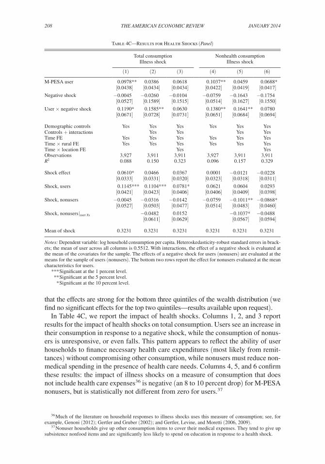
208 THE AMERICAN ECONOMIC REVIEW jANuARy 2014
that the effects are strong for the bottom three quintiles of the wealth distribution (we find no significant effects for the top two quintiles—results available upon request).
In Table 4C, we report the impact of health shocks. Columns 1, 2, and 3 report results for the impact of health shocks on total consumption. Users see an increase in their consumption in response to a negative shock, while the consumption of nonus-ers is unresponsive, or even falls. This pattern appears to reflect the ability of user households to finance necessary health care expenditures (most likely from remit-tances) without compromising other consumption, while nonusers must reduce non-medical spending in the presence of health care needs. Columns 4, 5, and 6 confirm these results: the impact of illness shocks on a measure of consumption that does not include health care expenses36 is negative (an 8 to 10 percent drop) for M-PESA nonusers, but is statistically not different from zero for users.37
36 Much of the literature on household responses to illness shocks uses this measure of consumption; see, for example, Genoni (2012); Gertler and Gruber (2002); and Gertler, Levine, and Moretti (2006, 2009).
37 Nonuser households give up other consumption items to cover their medical expenses. They tend to give up subsistence nonfood items and are significantly less likely to spend on education in response to a health shock.
Table 4C—Results for Health Shocks (Panel)
Total consumption Nonhealth consumptionIllness shock Illness shock
(1) (2) (3) (4) (5) (6)
M-PESA user 0.0978** 0.0386 0.0618 0.1037** 0.0459 0.0688*[0.0438] [0.0434] [0.0434] [0.0422] [0.0419] [0.0417]
Negative shock −0.0045 −0.0260 −0.0104 −0.0759 −0.1643 −0.1754[0.0527] [0.1589] [0.1515] [0.0514] [0.1627] [0.1550]
User × negative shock 0.1190* 0.1585** 0.0630 0.1380** 0.1641** 0.0780[0.0671] [0.0728] [0.0731] [0.0651] [0.0684] [0.0694]
Demographic controls Yes Yes Yes Yes Yes YesControls + interactions Yes Yes Yes YesTime FE Yes Yes Yes Yes Yes YesTime × rural FE Yes Yes Yes Yes Yes YesTime × location FE Yes YesObservations 3,927 3,911 3,911 3,927 3,911 3,911R2 0.088 0.150 0.323 0.096 0.157 0.329
Shock effect 0.0610* 0.0466 0.0367 0.0001 −0.0121 −0.0228[0.0333] [0.0331] [0.0320] [0.0323] [0.0318] [0.0311]
Shock, users 0.1145*** 0.1104*** 0.0781* 0.0621 0.0604 0.0293 [0.0421] [0.0423] [0.0406] [0.0406] [0.0409] [0.0398]
Shock, nonusers −0.0045 −0.0316 −0.0142 −0.0759 −0.1011** −0.0868*[0.0527] [0.0503] [0.0477] [0.0514] [0.0483] [0.0460]
Shock, nonusers | user Xs −0.0482 0.0152 −0.1037* −0.0488[0.0611] [0.0629] [0.0567] [0.0594]
Mean of shock 0.3231 0.3231 0.3231 0.3231 0.3231 0.3231
Notes: Dependent variable: log household consumption per capita. Heteroskedasticity-robust standard errors in brack-ets; the mean of user across all columns is 0.5512. With interactions, the effect of a negative shock is evaluated at the mean of the covariates for the sample. The effects of a negative shock for users (nonusers) are evaluated at the means for the sample of users (nonusers). The bottom two rows report the effect for nonusers evaluated at the mean characteristics for users.
*** Significant at the 1 percent level. ** Significant at the 5 percent level. * Significant at the 10 percent level.

209jack and suri: risk sharing and TransacTions cosTsVoL. 104 no. 1
B. Mechanisms
The most natural route by which M-PESA improves the ability of households to share risk is through remittances, but other mechanisms could be at work. For example, by providing a safe though unremunerated savings vehicle, it may induce households to build up precautionary savings balances. In this section, we confirm that the consumption smoothing effects documented above are due at least in part to risk-sharing arrangements between households that are implemented via remit-tances. We use the detailed survey data on remittances to estimate
(11) r ijt = α i + γ Shoc k ijt + μUse r ijt + βUse r ijt × Shoc k ijt
+ θ S X ijt × Shoc k ijt + θ M X ijt + η jt + π rt + ε ijt ,
where r ijt is a measure of remittances, and β is the coefficient of interest.Table 5A reports these results. Across the table, the relevant interaction term is
uniformly positive and significant, indicating that users who suffer negative shocks receive more remittances, in terms of the probability of receipt, the number received, and total revenue.38 To interpret these findings, the mean effects reported in the bottom rows suggest that for an average M-PESA user, a negative shock signifi-cantly increases the likelihood of receiving any remittances by 9 percentage points. Across all columns, the effects for users and nonusers are significantly different.
We find similar effects for the sample excluding Mombasa in columns 5 and 6 as well as for illness shocks as reported in columns 7 and 8. Lower transaction costs could lead to an increase or a decrease in the size of each remittance received: lower costs mean a larger share of any given transaction can reach the recipient, but they also make it economical to send smaller amounts more frequently. We find no effects of the impact of M-PESA on the average transaction size (results not reported).
Looking at magnitudes, from Tables 4B and 5A, we find that in the non-Nairobi sample, nonusers experience about a 6 percent larger drop in annual consumption as a result of income shocks. Users receive about KShs 1,000 extra39 over six months to help smooth risk—this amounts to about 4 percent of annual consumption, an amount close to the 6 percent difference between users and nonusers. We conduct two additional checks to show that savings are not the predominant mechanism—these results are reported in the online Appendix Tables 2 and 3. First, we show that the magnitude of risk sharing in the main specifications in the paper is smaller (and is no longer significant) if we control for remittances. Second, if we restrict our sample to rounds 3 and 4 where we collected data on savings amounts and focus just on Western Province,40 we find little evidence that savings respond differentially to income shocks for users and nonusers of M-PESA.
38 To reduce the influence of large values and bunching at zero we use the square root of the total amount received.
39 The effects reported in Table 5A are on the square root of remittances. The estimates in columns 5, 7, and 9 imply an effect on the level of remittances of between 900 and 1,100 KShs.
40 We restrict the sample to Western Province as we need variation in the use of M-PESA between the two rounds as the effects are identified from households that switch M-PESA use. By round 3, M-PESA had been adopted by 78 percent of our sample and by 86 percent in round 4. Western Province had the lowest adoption rates of 72 percent and 86 percent, respectively, for these two rounds.

210 THE AMERICAN ECONOMIC REVIEW jANuARy 2014
Next, motivated by our theory above, we investigate the impact of M-PESA on the size and nature of networks that people access when receiving support. The first measure of network access we use is the average distance that remittances received travel to reach a household. As reported in columns 1 and 2 of Table 5B, we find some evidence that such remittances originate from significantly greater distances for illness shocks.41
We also find that M-PESA allows households to reach deeper into their networks, as seen in columns 3 through 6. We examine this by constructing two measures of the number of active members in a network. The first is the number of different rela-tives or friends from whom remittances are received. Although we cannot precisely identify the individuals who sent remittances to a given household, we do know their relationship to the head of the receiving household, and their town/village of residence. We use this information to create unique relationship-town identifiers that provide a lower bound on the number of different people from whom a given
41 As a measure of distance, self-reported distances are extremely noisy (some are simply impossible). Instead, we used the reported town from which the remittance came, identified the town on a GIS database of towns or on Google Earth, and then computed distances. We were unable to find the towns for 10 percent of remittances in round 1 and 7 percent in round 2. The correlation between this calculated distance and self-reported distance is 0.85.
Table 5A—Mechanisms (Panel)
Overall shock: sample w/out Nairobi
Overall shock: w/out Mombasa Illness shock
Pr [receive]Number received
Total received
(square root) Pr [receive]
Total received
(square root) Pr [receive]
Total received
(square root)(1) (2) (3) (4) (5) (6) (7) (8)
M-PESA user 0.1897*** 0.1528*** 0.2574** 10.6757*** 0.1143** 9.0579** 0.1726*** 12.5548***[0.0456] [0.0487] [0.1305] [3.7863] [0.0517] [4.0683] [0.0420] [3.1596]
Negative shock −0.0442 −0.0409 −0.1306 1.8775 −0.1027 −1.8885 −0.1417 −9.3597[0.0390] [0.1438] [0.4193] [12.0864] [0.1452] [12.4371] [0.1457] [10.9683]
User × shock 0.0923* 0.1337** 0.3286* 8.3428* 0.1733*** 10.0472** 0.1598** 8.6003[0.0530] [0.0633] [0.1789] [4.6884] [0.0666] [4.9200] [0.0722] [5.2788]
Controls + interactions Yes Yes Yes Yes Yes Yes YesTime FE Yes Yes Yes Yes Yes Yes Yes YesTime × location FE Yes Yes Yes Yes Yes Yes Yes YesObservations 3,928 3,911 3,911 3,873 3,703 3,665 3,911 3,873R2 0.199 0.218 0.184 0.203 0.223 0.205 0.223 0.209
Shock effect 0.0066 0.0099 −0.0369 1.6647 0.0043 1.5026 0.0161 2.7412[0.0282] [0.0288] [0.0871] [2.2697] [0.0297] [2.3569] [0.0315] [2.5233]
Shock, users 0.0481 0.0478 0.0470 4.3755 0.0543 4.6901 0.0735* 6.5410*[0.0383] [0.0381] [0.1157] [3.4195] [0.0391] [3.5678] [0.0433] [3.5215]
Shock, nonusers −0.0442 −0.0366 −0.1400 −1.6403 −0.0561 −2.3154 −0.0544 −1.8914[0.0390] [0.0407] [0.1221] [2.6656] [0.0425] [2.7528] [0.0442] [3.0544]
Mean of user 0.5504 0.5512 0.5512 0.5494 0.5470 0.5450 0.5512 0.5494
Notes: Dependent variable: measures of household level remittances. Heteroskedasticity-robust standard errors in brackets. Total received (square root) refers to the square root of the total value of received remittances over the past six months. The reason for using the square root is that the total amount received has a long right tail as well as a number of zeros. In columns 5, 7, and 9, the effect on the level of remittances (not the square root) ranges from 900 to 1,100 KShs. Throughout, when Time × Location FE are included, Time × Rural FE are also included.
*** Significant at the 1 percent level. ** Significant at the 5 percent level. * Significant at the 10 percent level.

211jack and suri: risk sharing and TransacTions cosTsVoL. 104 no. 1
household receives remittances. The second measure of network size we construct is the ratio of this measure to the total potential network size for each household. To construct potential network size, we aggregate all the unique relationship-town combinations we observe in the data across all rounds and across both sending and receiving decisions. Using both these measures, we find that M-PESA helps house-holds reach deeper into their networks, as predicted by our model. M-PESA users are likely to receive remittances from more people (this holds for overall shocks and illness shocks), and they reach out to a larger fraction of their networks when they experience these income shocks.
C. Results Using Agent Data
In using the agent rollout data, we first estimate the reduced form difference-in-differences specification in equation (10). Tables 6A and 6B report these results for a number of different measures of agent access, and for the different types of shocks. The standard errors are clustered at the village level for all specifica-tions that use the agent data. The first access indicators are density measures—the
Table 5B—Where Do Remittances Come from: Distance and the Role of Networks (Panel)
log distance traveled
Number of different senders
Fraction of network remitting
Overall shock
Illness shock
Overall shock
Illness shock
Overall shock
Illness shock
(1) (2) (3) (4) (5) (6)
M-PESA user 0.0460 −0.0980 0.1783*** 0.2004*** 0.1012*** 0.1128***[0.4424] [0.3435] [0.0678] [0.0551] [0.0363] [0.0319]
Shock −0.2546 −0.2050 −0.3071 −0.4348* −0.0675 −0.1490[0.7437] [0.9028] [0.2160] [0.2227] [0.1279] [0.1252]
User × shock 0.2279 1.3929** 0.2008** 0.2519*** 0.0936* 0.1090*[0.5653] [0.6446] [0.0874] [0.0968] [0.0493] [0.0612]
Controls Yes Yes Yes Yes Yes YesControls + interactions Yes Yes Yes Yes Yes YesTime × location FE Yes Yes Yes Yes Yes YesObservations 1,518 1,518 3,911 3,911 3,394 3,394R2 0.484 0.488 0.194 0.199 0.241 0.246
Shock effect −0.3303 −0.2001 0.0249 0.0270 0.0125 0.0246[0.2166] [0.2355] [0.0439] [0.0457] [0.0221] [0.0236]
Shock, users −0.3076 0.0890 0.0852 0.1123* 0.0325 0.0484*[0.2563] [0.2764] [0.0580] [0.0606] [0.0247] [0.0270]
Shock, nonusers −0.4026 −1.1204** −0.0493 −0.0779 −0.0188 −0.0128[0.4150] [0.5099] [0.0594] [0.0620] [0.0384] [0.0441]
Mean of user 0.7609 0.7609 0.5512 0.5512 0.6104 0.6104
Notes: Dependent variable: measures of networks. Heteroskedasticity-robust standard errors in brackets. The number of different senders refers to the number of unique relationship-town combinations that households report receiv-ing remittances from in each round of the data. The fraction of the network divides this number by the total num-ber of unique relationship-town combinations ever seen in any round of the data, both on the sending side as well as on the receiving side. Throughout, when Time × Location FE are included, Time × Rural FE are also included.
*** Significant at the 1 percent level. ** Significant at the 5 percent level. * Significant at the 10 percent level.

212 THE AMERICAN ECONOMIC REVIEW jANuARy 2014
number of agents within 1, 2, 5, and 20 km of the household. Throughout, to account for the long right tail in the number of agents as well as some density at zero, we take the square root of the number of agents. The second measure of access to agents is the distance from the household to the closest agent (measured in log-meters).
Column 1 of Table 6A shows that households with better access to agents are less affected by negative shocks—the coefficients on the interaction between the 1 km agent density measure and the negative shock are positive. In column 2 we control for rural-by-time dummies and in column 3, we add location-by-time dummies, neither of which affects the estimated coefficient on the interaction. The results are similar for illness shocks. Columns 1 and 2 of Table 6B examine the responses to overall shocks using the 2 km agent density measure, with and without location-by-time dummies. The coefficient on the interaction term is similar across these speci-fications and similar in magnitude to the earlier columns. Columns 3 and 4 show results for the 5 km and the 20 km agent density measures, respectively. The coef-ficient on the interaction is significantly smaller in the 5 km case (though we lose some power when we include the rural-by-time dummies), and no different from zero in the 20 km case (this latter result also holds true if we use a 10 km density measure). In columns 5 and 6, we look at the distance to the closest agent. The coef-ficient on the interaction between this and the shock is negative as expected—the closer a household is to an agent the larger the offset on a negative shock (i.e., the better smoothed the shock). Overall, we find that better access to agents improves a household’s ability to smooth risk.
Table 6A—Reduced Forms Using Agent Rollout (Panel)
Overall shock Illness shock Agents w/in 1 km Agents w/in 1 km
(1) (2) (3) (4)
Negative shock −0.0525 −0.0543 −0.0543 −0.0591[0.0470] [0.0464] [0.0410] [0.0425]
Agents −0.0331 −0.0210 0.0450 0.0552[0.0400] [0.0382] [0.0377] [0.0381]
Agents × shock 0.0470** 0.0534*** 0.0451** 0.0350[0.0220] [0.0199] [0.0177] [0.0216]
Controls Yes Yes YesTime FE Yes Yes Yes YesTime × Location FE Yes YesTime × Rural FE Yes Yes Yes YesObservations 3,927 3,911 3,911 3,911R2 0.015 0.135 0.305 0.312
Shock effect 0.0002 0.0055 −0.0037 −0.0199[0.0346] [0.0332] [0.0328] [0.0346]
Mean of agents 1.1197 1.1206 1.1206 1.1206
Notes: Dependent variable: log household consumption per capita. Standard errors are clustered at the village level. For all columns, the negative shock effects are evaluated at the mean values of the agent variable. The dependent variable for the illness shock is nonmedical consumption per capita.
*** Significant at the 1 percent level. ** Significant at the 5 percent level. * Significant at the 10 percent level.

213jack and suri: risk sharing and TransacTions cosTsVoL. 104 no. 1
In Table 6C, we look at whether the agent rollout was associated with observ-ables in our data. In particular, we correlate the agent rollout with household wealth, ownership of a cell phone, measures of education of the household head, household access to various financial services, and the various income shocks. Although there are a few significant coefficients in Table 6B, we expect some to be significant just by chance. We find little evidence that the agent rollout is correlated with most household-level observables. However, two of the agent variables do correlate with the negative shock dummy, though the coefficients are economically small in mag-nitude (remember that the agent variables refer to measures of the number of agents within a given distance from a household and are not dummy variables). In the lower panel of the table, we correlate the agent rollout with the distance from the agent to Nairobi for two different agent access measures. Here, as the distance to Nairobi is fixed for a given household, we look at whether agent measures are correlated with the levels of agent access in round one as well as separately with the growth in agent access between the two rounds. We find little evidence of either.42
42 We use the GPS coordinates of the households and those of Nairobi to measure them. These are “as the crow flies” distances and not the actual distances traveled by road.
Table 6B—Reduced Forms Using Agent Rollout (Panel)
Overall shock
Agents w/in 2 km
Agents w/in 5 km
Agents w/in 20 km
Distance to closest agent
(1) (2) (3) (4) (5) (6)
Negative shock −0.0706 −0.0739 −0.0405 −0.0154 0.3317** 0.3398***[0.0530] [0.0460] [0.0464] [0.0559] [0.1353] [0.1294]
Agents −0.0232 0.0010 −0.0021 −0.0130 −0.0096 0.0151[0.0352] [0.0383] [0.0258] [0.0174] [0.0438] [0.0505]
Agents × Shock 0.0414** 0.0402*** 0.0130 0.0014 −0.0450** −0.0466***[0.0173] [0.0144] [0.0106] [0.0069] [0.0192] [0.0174]
Controls Yes Yes Yes YesTime FE Yes Yes Yes Yes Yes YesTime × Location FE Yes Yes Yes YesTime × Rural FE Yes Yes Yes Yes Yes YesObservations 3,927 3,911 3,911 3,911 3,927 3,911R2 0.016 0.305 0.301 0.300 0.016 0.304
Shock effect 0.0023 −0.0031 −0.0046 −0.0058 0.0012 −0.0026[0.0345] [0.0329] [0.0334] [0.0340] [0.0344] [0.0334]
Mean of agents 1.7613 1.7603 2.7539 6.7197 7.3486 7.3499
Notes: Dependent variable: log household consumption per capita. Standard errors are clustered at the village level. Distance to the closest agent is measured as the log of distance (distance measured in meters). For all columns, the negative shock effects are evaluated at the mean values of the agent variable. The coefficient on Agents × Shock interaction in column 1 is not significantly different if time × location fixed effects are included. Similarly, the coef-ficient on the Agents × Shock interaction in columns 2 through 4 are not significantly different if the time × loca-tion fixed effects are not included. The dependent variable for the illness shock is nonmedical consumption per capita.
*** Significant at the 1 percent level. ** Significant at the 5 percent level. * Significant at the 10 percent level.

214 THE AMERICAN ECONOMIC REVIEW jANuARy 2014
D. Falsification Test
Although we have strong reasons to believe that the agent rollout was not targeted to places that were systematically different from other areas, it remains a concern that the agents might have ended up being more heavily concentrated in areas where households were better able to smooth consumption in any case. To confirm that this possibility is not driving our results, we perform a falsification test using data from 1997 to 2007, before the launch of M-PESA.43 Apart from the period covered, the falsification strategy is identical to the first set of agent regressions reported in Table 6A. We match locational data on rainfall shocks and household consumption (see Suri 2012 for a full description) to two measures of subsequent agent access (the 2 km density and the distance to the nearest agent), and report the results in Table 7A.
This older survey was entirely rural, focused on agriculture and incomes, and did not collect complete consumption data, so we focus on the consumption of maize and other crops for this test. We include location and time dummies and a number of demographic controls in the specifications. Here, the shock is the deviation of rainfall from its longer term mean, and so, we expect the coefficient on the shock to be positive. Our results confirm that consumption is strongly correlated with rainfall shocks, but that there is no differential effect for households in locations
43 We thank Paul Ferraro for this suggestion.
Table 6C—Agent Rollout
Agents w/in 1 km Agents w/in 2 km Agents w/in 5 km Distance to agent
Coefficient SE Coefficient SE Coefficient SE Coefficient SE
log wealth 0.0047 [0.0088] 0.0155* [0.0093] −0.0079 [0.0123] 0.0079 [0.0061]Cell phone ownership −0.0288* [0.0175] 0.0074 [0.0232] −0.0184 [0.0286] 0.0040 [0.0180]Household size −0.0054 [0.0067] 0.0021 [0.0076] −0.0073 [0.0105] −0.0056 [0.0044]Fraction of boys in the household 0.0559 [0.0794] 0.1005 [0.0987] −0.0620 [0.1313] 0.0202 [0.0507]Fraction of girls in the household 0.0868 [0.0700] 0.1226 [0.0847] 0.3236* [0.1684] −0.0286 [0.0613]Occupation of head: farmer 0.0290 [0.0189] −0.0253 [0.0216] 0.0211 [0.0233] 0.0044 [0.0157]Occupation of head: professional 0.0082 [0.0304] 0.0420 [0.0391] −0.0037 [0.0413] 0.0184 [0.0196]Occupation of head: business −0.0409 [0.0276] 0.0232 [0.0302] 0.0226 [0.0418] −0.0009 [0.0200]Household head yrs of education −0.0033 [0.0021] −0.0008 [0.0026] 0.0040 [0.0031] −0.0018 [0.0014]HH has a bank account 0.0181 [0.0184] 0.0151 [0.0238] 0.0316 [0.0300] 0.0178 [0.0111]HH has a SACCO account 0.0011 [0.0237] −0.0061 [0.0276] 0.0327 [0.0505] −0.0042 [0.0185]HH has a ROSCA 0.0172 [0.0180] 0.0238 [0.0224] 0.0019 [0.0310] 0.0149 [0.0102]Negative shock 0.0120 [0.0151] 0.0393** [0.0183] 0.0492* [0.0258] −0.0035 [0.0120]Illness shock 0.0004 [0.0171] 0.0008 [0.0205] 0.0433 [0.0256] −0.0186 [0.0125]
Agents w/in 1 km
Agents w/in 2 km
Agents w/in 5 km
Distance to closest agent
Period 1 Changes Period 1 Changes Period 1 Changes Period 1 Changes
Distance to Nairobi −0.0009 0.0002 0.0026 −0.0011 −0.0029 0.0028 −0.0007 −0.0003[0.0031] [0.0013] [0.0058] [0.0028] [0.0028] [0.0028] [0.0056] [0.0011]
Notes: Dependent variable: measures of agent access. Standard errors are clustered at the village level. Distance to the closest agent is measured in log meters. Each row is a separate regression. In the top panel, all control for Time × Location and Time × Rural FE. In the bottom, all control for location dummies.
*** Significant at the 1 percent level. ** Significant at the 5 percent level. * Significant at the 10 percent level.

215jack and suri: risk sharing and TransacTions cosTsVoL. 104 no. 1
that subsequently experienced differential agent rollout. These findings hold for both measures of agent access that we use and provide evidence that unobserved heterogeneity does not contaminate our results. It is worth mentioning that these results are different from those in Suri (2012). She finds that households are able to smooth food consumption well—however, she finds this within villages, but she also finds that local risk sharing breaks down at higher levels of aggregation. We are looking at risk sharing within locations which are rather large, and so the results in Table 7A are illustrative of the results in Suri (2012) for higher levels of aggregation than the village.
In Table 7B, we use our M-PESA survey and restrict the sample as closely as we can to match the dataset used in the falsification test, by including only rural or agri-cultural households. In addition, we drop the top quintile of the income distribution, as the agricultural dataset does not include large commercial farmers. As shown in Table 7B, we can replicate the earlier results from Tables 4 through 6 for this subsample—indeed, if anything, the results are stronger. This lends further cred-ibility to the falsification test in Table 7A. In addition, it is worth noting that much as M-PESA does not help smooth food consumption on average (as in Table 4A), it does for this subsample of our households.
E. Attrition
Attrition is a concern with our panel given the high attrition rates, especially in Nairobi and other urban areas. To account for its potential effects, through-out all the results above, we controlled for rural by time dummies in addition to location-by-time dummies.44 In this section, we present some additional evidence
44 The rural-by-time dummies would fully eliminate attrition bias concerns in the extreme case where all nonran-dom attrition occurred between rural and urban areas for each time period, and all attrition within rural and urban
Table 7A—Falsification Test, 1997–2007
Agents w/in 2 km Distance to closest agent
Maize consumption Crop consumption Maize consumption Crop consumption
OLS Panel OLS Panel OLS Panel OLS Panel(1) (2) (3) (4) (5) (6) (7) (8)
Shock × agents −0.009 −0.058 0.091 0.055 0.070 0.088 −0.046 −0.037[0.083] [0.068] [0.085] [0.065] [0.077] [0.065] [0.072] [0.062]
Shock measure 0.418*** 0.412*** 0.400*** 0.377*** −0.175 −0.341 0.812 0.704 (positive measure) [0.074] [0.068] [0.069] [0.062] [0.648] [0.552] [0.608] [0.529]Agents −15.181 −13.537 44.036* 28.512
[16.855] [16.796] [24.018] [21.443]
Observations 4,736 4,736 4,736 4,736 4,736 4,736 4,736 4,736R2 0.323 0.345 0.486 0.546 0.324 0.345 0.486 0.546
Notes: Dependent variable: measures of log household consumption per capita. Heteroskedasticity robust standard errors in brackets. The shock measure used here is the deviation of main season rainfall from its long term mean. In addition, this specification controls for location and time dummies and measures of household demographics. All coefficients are multiplied by 1,000.
*** Significant at the 1 percent level. ** Significant at the 5 percent level. * Significant at the 10 percent level.

216 THE AMERICAN ECONOMIC REVIEW jANuARy 2014
that despite being large, attrition is not driving our results. We also present some robustness checks to try to account for the attrition. In Table 8A, we look at attri-tion directly and examine how the households that attrited differ from those that remain in the panel in period 1. We report results from multivariate regressions for the full sample and for the sample without Nairobi, with corresponding F statis-tics. Though there are differences between the households that attrited and those that did not, there is no difference in measured shocks or in agent access. In the analysis above, we control for all the observables (except M-PESA use) that dif-fer between the panel and nonpanel samples and their interactions with the shock. Below we present some additional checks to illustrate that attrition is not driving these results.
Even though the period 1 shocks are not correlated with future attrition, it may be the case that the shocks that happen between periods 1 and 2 drive attrition. To check this, we regressed the fraction of households that attrited in each commu-nity with the mean shock for that community. In the 237 communities in the data, this correlation is −0.054 and is not significant (the standard error is 0.047). We also present a subset of our results which have been reweighted using the strategy in Fitzgerald, Gottschalk, and Moffitt (1998)—henceforth, FGM—and show our
areas was random. While this extreme case does not hold, we think the rural-by-time dummies help absorb some of the nonrandom attrition by adjusting for the noticeably different attrition rates for rural and urban areas.
Table 7B—Falsification Test: Similar Sample for 2008–2009
Using M-PESA user status Using measures of agent access
Total consumption
Food consumption
Total consumption
Food consumption
Distanceto agent
Agents w/in 2 km
Distance to agent
Agentsw/in 2 km
(1) (2) (3) (4) (5) (6)
User/agent measure 0.0148 0.0012 0.0061 −0.0116 −0.0154 −0.0099[0.0628] [0.0563] [0.1074] [0.0631] [0.1108] [0.0650]
Negative Shock 0.1621 0.0191 0.7810*** 0.0698 0.7184*** −0.1193[0.1670] [0.1643] [0.2690] [0.1729] [0.2506] [0.1677]
User/Agent × Shock 0.1798** 0.0968 −0.0775*** 0.0873*** −0.0911*** 0.1045***[0.0803] [0.0828] [0.0291] [0.0242] [0.0260] [0.0231]
Controls + InteractionsTime × Location FE
YesYes
YesYes
YesYes
YesYes
YesYes
YesYes
ObservationsR2
1,8750.356
1,8740.383
1,8750.353
1,8750.356
1,8740.391
1,8740.396
Negative shock effect −0.0359 −0.0596 −0.0269 −0.0273 −0.0488 −0.0490[0.0411] [0.0381] [0.0415] [0.0411] [0.0378] [0.0373]
Shock, users 0.0302 −0.0114[0.0484] [0.0456]
Shock, nonusers −0.0934* −0.1014*[0.0560] [0.0539]
Notes: Heteroskedasticity-robust standard errors in brackets. All specifications control for the full set of covariates as above, their interactions with the shock and location by time dummies. Throughout, when Time × Location FE are included, Time × Rural FE are also included.
*** Significant at the 1 percent level. ** Significant at the 5 percent level. * Significant at the 10 percent level.

217jack and suri: risk sharing and TransacTions cosTsVoL. 104 no. 1
results are robust to this. We report these results in columns 1, 2, and 3 of Table 8B. Also in Table 8B we report a subset of results for the set of 146 communities where attrition is less than about 20 percent at the community level (that is, of the approxi-mately ten households to be interviewed per community, at least eight were found). The overall attrition in this sample is only 7 percent. As can be seen, our main results hold for this subsample.
F. IV Results
We instrument for the use of M-PESA and its interaction with the income shock using two agent access variables (distance to the closest agent and the number of agents within 5 km of the household) and their interactions with the income shock.45
45 For the purposes of efficiency, one might argue we should use as many indicators of agent access and their interactions with the shocks as possible. However, as the access indicators are highly collinear, we restrict ourselves to the two mentioned above.
Table 8A—Correlates of Nonattrition
Full sample
WithoutNairobi
Full sample
Without Nairobi
log total expenditure −0.0125 −0.0127 Years of education of −0.0002 0.0012[0.0188] [0.0199] HH Head [0.0019] [0.0020]
M-PESA user 0.0337 0.0191 Occupation—farmer 0.0453 0.0438[0.0243] [0.0260] [0.0305] [0.0314]
Cell phone ownership 0.0467* 0.0544** Occupation—professional 0.0263 0.0169[0.0249] [0.0257] [0.0306] [0.0336]
log distance to agent −0.0025 −0.0112 Occupation—househelp −0.0150 −0.0170[0.0152] [0.0177] [0.0404] [0.0446]
Agents within 1 km −0.0092 −0.0074 Occupation—run a business 0.0363 0.0309[0.0152] [0.0165] [0.0331] [0.0350]
Agents within 2 km −0.0155 −0.0322* Occupation—sales 0.1001* 0.0860[0.0123] [0.0181] [0.0535] [0.0563]
Agents within 5 km 0.0036 0.0036 HH has a bank account 0.0231 0.0197[0.0080] [0.0140] [0.0226] [0.0236]
Negative shock 0.0081 0.0140 HH has a ROSCA account 0.0033 0.0104[0.0238] [0.0255] [0.0280] [0.0295]
Illness shock 0.0091 0.0153 HH has a SACCO 0.0116 0.0131[0.0266] [0.0281] [0.0200] [0.0210]
Sent remittance 0.0008 −0.0007 Household size 0.0141** 0.0143**[0.0213] [0.0227] [0.0055] [0.0058]
Received remittance −0.0192 −0.0163 Urban dummy −0.0887** −0.0791**[0.0217] [0.0229] [0.0366] [0.0377]
Observations 2,998 2,518R2 0.168 0.176F-Statistic [ p-value] 2.469
[0.0002]2.577[0.0001]
Notes: Dependent variable is a dummy variable for the household remaining in the panel sample. Heteroskedasticity-robust standard errors in brackets. All regressions control for location dummies.
*** Significant at the 1 percent level. ** Significant at the 5 percent level. * Significant at the 10 percent level.

218 THE AMERICAN ECONOMIC REVIEW jANuARy 2014
Table 9 presents these results for both consumption and remittance variables. Throughout this table, we control for our standard set of covariates as above. We do not include the location-by-time dummies. The first stage for predicting M-PESA use with the agent rollout is not precise when we include these location-by-time dummies, as they soak up a lot of the variation we would like to include (i.e., the growth of agents and the growth of M-PESA use over time). However, we do still control for rural-by-time dummies, and the results hold up, especially when we look at the sample excluding Mombasa.
In Table 9, we show the cross-section estimates in column 1, and in columns 2 through 8 we present the various panel versions. For space reasons, we do not show the first-stage regressions in Table 9, but we report the Kleibergen-Paap statistics, both the asymptotic LM test for underidentification (and its correspond-ing p-value) and the F-statistic Wald test (where the Kleibergen-Paap idea is used to generalize the Stock-Yogo/Donald-Cragg test statistic to allow for clustered standard errors).46 For the Wald test, when there are two endogenous variables and
46 With i.i.d. errors, we can perform a Hausman test to compare the OLS (or the fixed effects) and IV regressions. We do not report these results in the paper, but we are unable to reject the null that the coefficients underlying the two specifications are the same. From these Hausman test results, therefore, the estimates in Tables 4A and 5A are preferred as they are efficient under the null.
Table 8B—Further Results on Attrition (Results for overall shock)
FGM weights Limited sample where attrition is low at community level
M-PESA user Dist toagent M-PESA user
Agents w/in 1 km
Dist to agent
Total consumption
Pr[receive]
Total consumption
Total consumption
Pr[receive]
Total received
Total consumption
(1) (2) (3) (4) (5) (6) (7) (8)
User/agent 0.0036 0.1675*** 0.0188 −0.0594 0.0994* 8.7203** 0.0739 0.0268 measure [0.0472] [0.0477] [0.0534] [0.0580] [0.0581] [4.2328] [0.0566] [0.0598]Negative shock 0.1761 −0.0111 0.5503*** 0.2015 −0.1031 −4.5028 0.1825 0.8997***
[0.1639] [0.1405] [0.2100] [0.1750] [0.1967] [13.0864] [0.1793] [0.2421]User/agent 0.1305** 0.1232** −0.0499*** 0.2469*** 0.2380*** 13.8458*** 0.0843***−0.0876*** × shock [0.0632] [0.0627] [0.0183] [0.0740] [0.0753] [5.2629] [0.0267] [0.0242]
Controls + interactions
Yes Yes Yes Yes Yes Yes Yes Yes
Time × location FE
Yes Yes Yes Yes Yes Yes Yes Yes
Observations 3,893 3,893 3,893 2,789 2,789 2,761 2,789 2,789R2 0.326 0.224 0.326 0.357 0.240 0.228 0.357 0.357
Shock effect −0.0034 0.0100 0.0004 −0.0007 0.0015 1.7150 0.0035 0.0082[0.0296] [0.0286] [0.0295] [0.0335] [0.0346] [2.5152] [0.0332] [0.0334]
Shock, users 0.0383 0.0431 0.0815** 0.0660 6.0644[0.0379] [0.0377] [0.0414] [0.0454] [3.7894]
Shock, −0.0548 −0.0307 −0.0844* −0.0641 −2.6646 nonusers [0.0440] [0.0400] [0.0508] [0.0484] [3.0531]Shock, non- −0.0922* −0.0802 −0.1655*** −0.1720***−7.7814* users |user X’s [0.0534] [0.0530] [0.0636] [0.0645] [4.4042]
Notes: Heteroskedasticity-robust standard errors in brackets. Columns 1–3 report results from reweighting the data as per Fitzgerald, Gottschalk, and Moffitt (1998) to account for attrition. Throughout, when Time × Location FE are included, Time × Rural FE are also included.
*** Significant at the 1 percent level. ** Significant at the 5 percent level. * Significant at the 10 percent level.

219jack and suri: risk sharing and TransacTions cosTsVoL. 104 no. 1
four instruments, Stock, Wright, and Yogo (2002) suggest a test statistic critical value of 11. Across most specifications, the Kleibergen-Paap test statistics reject the null (we lose power for the specifications with rural-by-time dummies though the estimates of the effects are similar). Overall, we find results consistent with our earlier findings. M-PESA users are better able to smooth shocks, and we find that these improvements come about due to increased remittances.
VI. Conclusion
In the presence of high transaction costs, the risk-sharing benefits of geographic sep-aration and income diversification can go unrealized. Small idiosyncratic risks might be shared within local networks, but larger and more aggregate shocks are likely to affect consumption directly. In this article we test the importance of transaction costs as a barrier to full insurance in the context of the rapid expansion of a cost-reducing innovation in Kenya, M-PESA—a cell phone–based money transfer product that has been adopted by a large majority of households in less than four years. The potential
Table 9—IV Results (Cross section and Panel)
Total consumption Pr [Receive]
Cross section Panel Panel Panel Panel Panel Panel Panelw/out Msa w/out Msa w/out Msa w/out Msa
(1) (2) (3) (4) (5) (6) (7) (8)
M-PESA user −0.4705* −0.5128*** −0.6328*** −0.6730*** −0.3155 −0.2561 −0.1455 0.0849[0.2685] [0.1885] [0.1851] [0.2039] [0.8549] [1.5697] [0.1741] [1.1219]
Negative shock −0.3344** −0.3601** −0.3462** −0.4372** −0.3762** −0.4549** −0.1739 −0.1395[0.1469] [0.1668] [0.1602] [0.1741] [0.1547] [0.2095] [0.1584] [0.1718]
User × shock 0.5124* 0.6146** 0.5992** 0.7619** 0.6782** 0.8180** 0.3862 0.3080[0.2653] [0.2908] [0.2771] [0.3084] [0.2679] [0.3655] [0.2732] [0.2903]
Controls Yes Yes Yes Yes Yes Yes YesRural × time FE Yes Yes YesLocation + Rural FE
Yes
Observations 3,911 3,926 3,894 3,688 3,894 3,688 3,688 3,688
Shock effect −0.0519** −0.0217 −0.0159 −0.0204 −0.0024 −0.0074 0.0373 0.0290[0.0264] [0.0365] [0.0346] [0.0359] [0.0314] [0.0333] [0.0302] [0.0313]
Shock, users 0.1781 0.2545* 0.2530** 0.3247** 0.3020** 0.3631** 0.2123* 0.1685[0.1237] [0.1331] [0.1255] [0.1427] [0.1205] [0.1618] [0.1212] [0.1246]
Shock, nonusers −0.3344** −0.3601** −0.3462** −0.4372** −0.3762** −0.4549** −0.1739 −0.1395[0.1469] [0.1668] [0.1602] [0.1741] [0.1547] [0.2095] [0.1584] [0.1718]
Kleibergen-Paap LM test
39.7957 46.6806 48.2429 45.2436 3.7324 1.7344 45.2436 1.7344
LM test p-value 0.0000 0.0000 0.0000 0.0000 0.2919 0.6293 0.0000 0.6293
Kleibergen-Paap F statistic
9.3904 12.3462 12.7063 12.5678 0.9262 0.4258 12.5678 0.4258
(critical value = 11)
Notes: Heteroskedasticity-robust standard errors in brackets. The excluded instruments are distance to the closest agent and the number of agents within 5 km of the household and interactions of each of these with the negative shock. None of these specifications controls for location by time fixed effects. The cross-section results include location fixed effects.
*** Significant at the 1 percent level. ** Significant at the 5 percent level. * Significant at the 10 percent level.
220 THE AMERICAN ECONOMIC REVIEW jANuARy 2014
for mobile technology, and mobile money specifically, to transform the lives of the poor, while palpable, is so far little documented. In this paper, we present convincing evidence that mobile money has had a significant impact on the ability of households to share risk, and this is attributable to the associated reduction in transaction costs. The results are robust across various specifications and also when we use data on the rollout of M-PESA agents across the country, which provides an additional source of exogenous variation in access to the service. We find that households who do not use the technology suffer a 7 percent drop in consumption when hit by a negative shock, while the consumption of households who use M-PESA is unaffected.
Such insurance is valuable in itself—indeed, the probability of shocks and their size suggest a back of the envelope calculation of welfare benefits of on average 3 to 4 percent of income, depending of course on attitudes towards risk. The longer term welfare benefits could be higher, if the dynamics of poverty are driven by ran-dom reductions in consumption that lead to persistently low income (Dercon 2006). Over the longer term, as electronic payments mature and facilitate more frequent and better matched trades, the impact of this financial innovation on the level of consumption, as well as its variance, could be significant. As M-PESA and other mobile money applications are adopted by a broad cross-section of businesses, pro-ductivity and efficiency gains could be realized, as had been the case following the diffusion of computing technology in the United States (for examples, see Bosworth and Triplett 2002 and Brynjolfsson and Hitt 2003).
Although the technology also provides a convenient and safe method of saving, which could facilitate self-insurance, we find that an important mechanism that lies behind the improved risk spreading is remittances. When faced with a shock, house-holds with access to the technology are more likely to receive a remittance; they receive a greater number of remittances and larger amounts of money in total. In addition, the remittances they receive come from further afield and from a larger sample of network members. These results highlight the importance of transaction costs when using social networks to smooth risk. Mobile money appears to increase the effective size of, and number of active participants in, risk-sharing networks, seemingly without exacerbating information, monitoring, and commitment costs.
This observation suggests a reappraisal of competing explanations for incomplete risk spreading in informal networks in developing countries, which have focused on problems of asymmetric information and limited commitment. We find no evidence that the associated constraints are weaker for users of M-PESA than for nonusers—indeed, active members of insurance networks of M-PESA users are more geographi-cally dispersed, suggesting that if anything, information problems may be more acute and social pressures that enforce commitment to ongoing relationships may be less effective for users than for nonusers. In this case, the benefits of the lower transac-tion costs of M-PESA appear to be sufficiently large to offset any incompleteness of insurance that would otherwise arise from information or commitment problems. Overall, the welfare implications of M-PESA are unclear. Much as it has resulted in improved risk sharing as documented in this article, it may also impose costs. There is a literature showing that kinship networks can impose costs on their network by over-taxing them with requests and therefore forcing them to hide their income or wealth (see Baland, Guirkinger, and Mali 2011). The reduction in transaction costs that M-PESA provides could make such requests for transfers easier and more common.

221jack and suri: risk sharing and TransacTions cosTsVoL. 104 no. 1
REFERENCES
Aker, Jenny C. 2010. “Information from Markets Near and Far: Mobile Phones and Agricultural Mar-kets in Niger.” American Economic Journal: Applied Economics 2 (3): 46–59.
Aker, Jenny C., and Isaac M. Mbiti. 2010. “Mobile Phones and Economic Development in Africa.” Journal of Economic Perspectives 24 (3): 207–32.
Alderman, Harold, Jere R. Behrman, Hans-Peter Kohler, John A. Maluccio, and Susan Cotts Watkins. 2001. “Attrition in Longitudinal Household Survey Data: Some Tests for Three Developing-Country Samples.” Unpublished.
Ambrus, Attila, Markus Mobius, and Adam Szeidl. 2010. “Consumption Risk-sharing in Social Net-works.” Unpublished.
Angelucci, Manuela, Giacomo De Giorgi, Marcos Rangel, and Imran Rasul. 2009. “Insurance and Investment Within Family Networks.” Unpublished.
Ashraf, Nava, Diego Aycinena, Claudia Martínez A., and Dean Yang. 2011. “Remittances and the Prob-lem of Control: A Field Experiment Among Migrants from El Salvador.” Unpublished.
Attanasio, Orazio P., and Nicola Pavoni. 2011. “Risk Sharing in Private Information Models with Asset Accumulation: Explaining the Excess Smoothness of Consumption.” Econometrica 79 (4): 1027–68.
Attanasio, Orazio, Luca Pellerano, and Sandra Polania Reyes. 2009. “Building Trust? Conditional Cash Transfer Programmes and Social Capital.” Fiscal Studies 30 (2): 139–77.
Aycinena, Diego, Claudia Martínez A., and Dean Yang. 2010. “The Impact of Remittance Fees on Remittance Flows: Evidence from a Field Experiment Among Salvadorian Migrants.” Unpublished.
Baird, Sarah, Joan Hamory, and Edward Miguel. 2008. “Tracking, Attrition and Data Quality in the Kenyan Life Panel Survey Round 1 (KLPS-1).” Unpublished.
Baland, Jean-Marie, Catherine Guirkinger, and Charlotte Mali. 2011. “Pretending to Be Poor: Bor-rowing to Escape Forced Solidarity in Cameroon.” Economic Development and Cultural Change 60 (1): 1–16.
Bloch, Francis, Garance Genicot, and Debraj Ray. 2008. “Informal Insurance in Social Networks.” Journal of Economic Theory 143 (1): 36–58.
Blumenstock, Joshua, Nathan Eagle, and Marcel Fafchamps. 2011. “Charity and Reciprocity in Mobile Phone-Based Giving: Evidence from Rwanda.” Unpublished.
Blundell, Richard, Luigi Pistaferri, and Ian Preston. 2008. “Consumption Inequality and Partial Insur-ance.” American Economic Review 98 (5): 1887–921.
Bosworth, Barry P., and Jack Triplett. 2002. “‘Baumol’s Disease’ has been Cured: IT and Multifactor Productivity in U.S. Services Industries.” http://www.brookings.edu/es/research/projects/productiv-ity/workshops/20020517_triplett.pdf (accessed November 2013).
Brynjolfsson, Erik, and Lorin M. Hitt. 2003. “Computing Productivity: Firm-Level Evidence.” Review of Economics and Statistics 85 (4): 793–808.
Chiappori, Pierre-Andre, Krislert Samphantharak, Sam Schulhofer-Wohl, and Robert M. Townsend. 2011. “Heterogeneity and Risk Sharing in Village Economies.” Unpublished.
Coate, Stephen, and Martin Ravallion. 1993. “Reciprocity without Commitment: Characterization and Performance of Informal Insurance Arrangements.” Journal of Development Economics 40 (1): 1–24.
Cochrane, John H. 1991. “A Simple Test of Consumption Insurance.” Journal of Political Economy 99 (5): 957–76.
Communications Commission of Kenya (CCK). 2011. Quarterly Sector Statistics Report, Second Quarter, October–December 2010/2011. Nairobi, Kenya: CCK.
Deaton, Angus. 1990. “On Risk, Insurance, and Intra-Village Consumption Smoothing.” Unpublished.Deaton, Angus. 1992. “Saving and Income Smoothing in Cote d’Ivoire.” Journal of African Econo-
mies 1 (1): 1–24.Deaton, Angus. 1997. The Analysis of Household Surveys: A Microeconometric Approach to Develop-
ment Policy. Baltimore: Johns Hopkins University Press.Dercon, Stefan. 2006. “Vulnerability: A Micro Perspective.” Oxford University, Queen Elizabeth
House (QEH) Working Paper 149.Dercon, Stefan, and Joseph S. Shapiro. 2007. “Moving On, Staying Behind, Getting Lost: Lessons on
Poverty Mobility from Longitudinal Data.” In Moving Out of Poverty: Cross-Disciplinary Perspec-tives, edited by D. Narayan and P. Petesch, 77–126. Washington, DC: World Bank.
De Weerdt, Joachim, and Stefan Dercon. 2006. “Risk-Sharing Networks and Insurance Against Ill-ness.” Journal of Development Economics 81 (2): 337–56.
Fafchamps, Marcel, and Flore Gubert. 2007. “The Formation of Risk Sharing Networks.” Journal of Development Economics 83 (2): 326–50.

222 THE AMERICAN ECONOMIC REVIEW jANuARy 2014
Fafchamps, Marcel, and Susan Lund. 2003. “Risk-Sharing Networks in Rural Philippines.” Journal of Development Economics 71 (2): 261–87.
Fitzgerald, John, Peter Gottschalk, and Robert Moffitt. 1998. “An Analysis of Sample Attrition in Panel Data: The Michigan Panel Study of Income Dynamics.” Journal of Human Resources 33 (2): 251–99.
Genicot, Garance, and Debraj Ray. 2003. “Group Formation in Risk-Sharing Arrangements.” Review of Economic Studies 70 (1): 87–113.
Genoni, Maria Eugenia. 2012. “Health Shocks and Consumption Smoothing: Evidence from Indone-sia.” Economic Development and Cultural Change 60 (3): 475–506.
Gertler, Paul, and Jonathan Gruber. 2002. “Insuring Consumption Against Illness.” American Eco-nomic Review 92 (1): 51–76.
Gertler, Paul, David I. Levine, and Enrico Moretti. 2006. “Is Social Capital the Capital of the Poor? The Role of Family and Community in Helping Insure Living Standards against Health Shocks.” CESifo Economic Studies 52 (3): 455–99.
Gertler, Paul, David I. Levine, and Enrico Moretti. 2009. “Do Microfinance Programs Help Families Insure Consumption against Illness?” Health Economics 18 (3): 257–73.
Goldstein, Markus. 1999. “Chop Time, No Friends: Examining Options for Individual Insurance in Southern Ghana.” Unpublished.
Grimard, Franque. 1997. “Household Consumption Smoothing through Ethnic Ties: Evidence from Cote D’Ivoire.” Journal of Development Economics 53 (2): 391–422.
Haas, Sherri, Megan Plyler, and Geetha Nagarajan. 2010. “Outreach of M-PESA System in Kenya: Emerging Trends.” Unpublished.
Hayashi, Fumio, Joseph Altonji, and Laurence Kotlikoff. 1996. “Risk-Sharing between and within Families.” Econometrica 64 (2): 261–94.
Heeringa, Steven. 1997. “Russia Longitudinal Monitoring Survey (RLMS) Sample Attrition, Replen-ishment, and Weighting in Rounds V-VII.” Unpublished.
Jack, William, and Tavneet Suri. 2011. “Mobile Money: The Economics of M-PESA.” National Bureau of Economic Research Working Paper 16721.
Jack, William, and Tavneet Suri. 2014. “Risk Sharing and Transactions Costs: Evidence from Kenya’s Mobile Money Revolution: Dataset.” American Economic Review. http://dx.doi.org/10.1257/aer.104.1.183.
Jack, William, Tavneet Suri, and Robert Townsend. 2010. “Monetary Theory and Electronic Money: Reflections on the Kenyan Experience.” Federal Reserve Bank of Richmond Economic Quarterly 96 (1): 83–122.
Jackson, Matthew O. 2009. “Networks and Economic Behavior.” Annual Review of Economics 1 (1): 489–511.
Jackson, Matthew O. 2010. “An Overview of Social Networks and Economic Applications.” In The Handbook of Social Economics. Vol. 1, edited by J. Benhabib, A. Bisin, and M.O. Jackson, 511–85. Amsterdam: Elsevier, North-Holland.
Jensen, Robert. 2007. “The Digital Provide: Information (Technology), Market Performance, and Wel-fare in the South Indian Fisheries Sector.” Quarterly Journal of Economics 122 (3): 879–924.
Ivatury, Gautam, and Mark Pickens. 2006. Mobile Phone Banking and Low-Income Customers: Evi-dence from South Africa. Washington, DC: Consultative Group to Assist the Poor.
Kaplan, Greg. 2006. “The Cross-Sectional Implications of Incomplete Markets: Private Information or Limited Enforcement?” Unpublished.
Kinnan, Cynthia. 2010. “Distinguishing Barriers to Insurance in Thai Villages.” Unpublished.Kinnan, Cynthia, and Robert Townsend. 2010. “Kinship and Financial Networks, Formal Financial
Access, and Risk Reduction.” Unpublished.Lam, David, Cally Ardington, and Murray Leibbrandt. 2007. “Schooling as a Lottery: Racial Differ-
ences in School Advancement in Urban South Africa.” Unpublished. Ligon, Ethan. 1998. “Risk Sharing and Information in Village Economics.” Review of Economic Stud-
ies 65 (4): 847–64.Ligon, Ethan, Jonathan P. Thomas, and Tim Worrall. 2002. “Informal Insurance Arrangements with
Limited Commitment: Theory and Evidence from Village Economies.” Review of Economic Stud-ies 69 (1): 209–44.
Mace, Barbara J. 1991. “Full Insurance in the Presence of Aggregate Uncertainty.” Journal of Politi-cal Economy 99 (5): 928–56.
Mas, Ignacio. 2009. “The Economics of Branchless Banking.” Innovations 4 (2): 57–75.Mas, Ignacio, and Kabir Kumar. 2008. “Banking on Mobiles: Why, How, for Whom?” Consultative
Group to Assist the Poor (CGAP), Focus Note No. 48.Mas, Ignacio, and Olga Morawczynski. 2009. “Designing Mobile Money Services: Lessons from
M-PESA.” Innovations 4 (2): 77–91.

223jack and suri: risk sharing and TransacTions cosTsVoL. 104 no. 1
Mas, Ignacio, and Sarah Rotman. 2008. “Going Cashless at the Point of Sale: Hits and Misses in Developed Countries.” Consultative Group to Assist the Poor (CGAP), Focus Note No. 51.
Morawczynski, Olga. 2008. “Surviving in the ‘Dual System’: How M-PESA is Fostering Urban-to-Rural Remittances in a Kenyan Slum.” Unpublished.
Morawczynski, Olga, and Mark Pickens. 2009. “Poor People Using Mobile Financial Services: Obser-vations on Customer Usage and Impact from M-PESA.” Unpublished.
Phelan, Christopher. 1998. “On the Long Run Implications of Repeated Moral Hazard.” Journal of Economic Theory 79 (2): 174–91.
Plyler, Megan, Sherri Haas, and Geetha Nagarajan. 2010. “Community-Level Economic Effects of M-PESA in Kenya: Initial Findings.” Unpublished.
Rao, Madanmohan. 2011. “Mobile Africa Report 2011: Regional Hubs of Excellence and Innovation.” http://www.mobilemonday.net/reports/MobileAfrica_2011.pdf (accessed November 2013).
Rosenzweig, Mark R., and Oded Stark. 1989. “Consumption Smoothing, Migration, and Marriage: Evidence from Rural India.” Journal of Political Economy 97 (4): 905–26.
Schulhofer-Wohl, Sam. 2011. “Heterogeneity and Tests of Risk Sharing.” Journal of Political Economy 119 (5): 925–58.
Stock, James H., Jonathan H. Wright, and Motohiro Yogo. 2002. “A Survey of Weak Instruments and Weak Identification in Generalized Method of Moments.” Journal of Business and Economic Sta-tistics 20 (4): 518–29.
Suri, Tavneet. 2012. “Estimating the Extent of Risk Sharing Between Households.” Unpublished.Suri, Tavneet. 2011. “Selection and Comparative Advantage in Technology Adoption.” Econometrica
79 (1): 159–209.Thomas, Duncan, Firman Witoelar, Elizabeth Frankenberg, Bondan Sikoki, John Strauss, Cecep
Sumantri, Wayan Suriastini. 2012. “Cutting the Costs of Attrition: Results from the Indonesia Fam-ily Life Survey.” Journal of Development Economics 98 (1): 108–23.
Thomas, Jonathan, and Tim Worrall. 1990. “Income Fluctuation and Asymmetric Information: An Example of a Repeated Principal-Agent Problem.” Journal of Economic Theory 51 (2): 367–90.
Townsend, Robert M. 1994. “Risk and Insurance in Village India.” Econometrica 62 (3): 539–91.Townsend, Robert M. 1995. “Consumption Insurance: An Evaluation of Risk-Bearing Systems in
Low-Income Economies.” Journal of Economic Perspectives 9 (3): 83–102.Udry, Christopher. 1994. “Risk and Insurance in a Rural Credit Market: An Empirical Investigation in
Northern Nigeria.” Review of Economic Studies 61 (3): 495–526.Yang, Dean, and HwaJung Choi. 2007. “Are Remittances Insurance? Evidence from Rainfall Shocks
in the Philippines.” World Bank Economic Review 21 (2): 219–48.