Risk Measures with Normal Distributed Black Options ...janroman.dhis.org/stud/EXJOBB/Huang.pdf ·...
63
Mälardalen University, Västerås, Sweden, 2013 -06 -05 School of Education, Culture and Communication Division of Applied Mathematics Bachelor Degree Project in Financial Mathematics Risk Measures with Normal Distributed Black Options Pricing Model Supervisors: Anatoliy Malyarenko, Jan Röman Author: Wenqing Huang
Transcript of Risk Measures with Normal Distributed Black Options ...janroman.dhis.org/stud/EXJOBB/Huang.pdf ·...

Mälardalen University, Västerås, Sweden, 2013 -06 -05
School of Education, Culture and Communication
Division of Applied Mathematics
Bachelor Degree Project in Financial Mathematics
Risk Measures with Normal Distributed
Black Options Pricing Model
Supervisors: Anatoliy Malyarenko, Jan Röman
Author: Wenqing Huang
Acknowledgements
I would like to express my great gratitude to my supervisors Anatoliy Malyarenko and
Jan R.M. Röman for the great guidance they rendered to me through their comments
and thoughts. Not only did they help me in this thesis, they also gave me a good
foundation through their lectures. A special appreciation to the other lecturers in the
Division of Applied Mathematics of Mälardalen University, their lectures have been
of great help in the realization of this thesis as well.
2
Abstract
The aim of the paper is to study the normal Black model against the classical Black
model in a trading point of view and from a risk perspective. In the section 2, the
derivation of the model is subject to the assumption that implementation of a dynamic
hedging strategy will eliminate the risk of holding long or short positions in such
options. In addition, the derivation of the formulas has been proved mathematically by
the notable no-arbitrage argument. The idea of the theory is that the fair value of any
derivative security is computed as the expectation of the payoff under an equivalent
martingale measure. In the third section, the Greeks have been derived by
differentiation. Also brief explanation regarding how one can approximate log-normal
Black with normal version has been explored in the section 4. Eventually, with the aid
of Excel VBA, there is an empirical test for swaptions on an At-The-Money volatility
surface, given as Black (log-normal) volatilities, which is translated into a normal
volatility surface. Then calculate and plot how delta and vega differs between the
models.
Key Words: Black model, Normal Black model, Interest rate derivatives, Forward swap rate, Swaptions, Volatilities, Greeks, Yield curve, Risk disparities
3

Contents
1. Introduction .................................................................................................................................5
1.1. Negative interest rates......................................................................................................5
1.2. Notations and assumptions..............................................................................................6
1.3. A short review of the literature on the Black option pricing model .............................7
1.4. Problem formulation........................................................................................................8
2. Derivation of equation and formulas.......................................................................................10
3. Risk measures ............................................................................................................................13
3.1. Delta ................................................................................................................................14
3.2. Gamma............................................................................................................................16
3.3. Vega .................................................................................................................................17
3.4. Theta and Rho ................................................................................................................18
4. Equivalence between the normal and the lognormal implied volatility ...............................19
4.1 Singular perturbation expansion ...................................................................................20
4.2 Conversion between log normal and normal volatility ................................................21
5. Empirical test on disparities between Black model and normal Black model.....................21
6.Conclusion ..................................................................................................................................25
7. Reference....................................................................................................................................27
Appendix ........................................................................................................................................29
Table 1: Risk measures for the Black model .......................................................................29
2. Black formulas expressed for Caps/Floors and Swaptions & annuity factor ..............30
3. Presentation of input-output interfaces...........................................................................32
4. Extract of VBA program codes........................................................................................33
5. Summary of reflection of objectives in the thesis ...........................................................36
4

1. Introduction
1.1. Negative interest rates
When it comes to the question regarding how low interest rates can reach, both the
economists and traders around the globe believe that interest rates could go negative.
Although that sounds unbelievable, there are precedents for negative interest rates.
To name just a few macroeconomic cases, in the late 1990s zero interest rate came
into being briefly, as Japanese savers were so unsecured about the stock market which
had collapsed, they would rather deposit their money in the bank even at a negative
interest rate. In 2009, Sweden’s Riksbank, the first central bank to adopt negative
interest rates, actually lowered its deposit rate to a -0.25% in the midst of the financial
crisis. On a regular basis, negative real interest rates, when nominal interest rates are
below inflation rate, become a monetary policy tool of the governments to tax on
money as a mean of driving money out of the banks and into investments to benefit
the economy, as well as dealing with variables like inflation and unemployment.
In the financial market, another example of a negative interest rate, a rate below zero
whereby the lender pays interest to the borrower, is a private placement with
institutional investor of debt-plus-warrants, a security called Squarz from Berkshire
Hathaway Corporation governed by the Wall Street legend Warren Buffett. Goldman
Sachs engineered the structure in mid-2002, and called it the “first ever
negative-coupon security.” With the aid of high stock market volatility and low
market interest rates, Berkshire would pay around 3% annually on the bonds being
issued. Instead the investor would receive a warrant allowing the purchase of
Berkshire stock as well, and to keep the warrant alive, investors would have to pay a
higher rate, perhaps 3.75%, meanwhile Berkshire made the interest payments. To sum
up, the net effect amounted to a negative interest rate.
In recent decades, the interest rate derivative instruments, which are products whose
payoffs depend in some way on the level of interest rate, are increasingly arousing
5

interest from either such institutional investors as banks or individual investors with
customized cashflow demands or as a speculative tool to profit from their specific
views on the movement of the market interest rates, say directional movements or
volatility movements.
1.2. Notations and assumptions
For the whole paper, denote the current future price f, with -∞ < f < ∞. For
instruments like swaptions, f stands for the forward rates which are the rates of
interest implied by current zero rates for periods of time in the future. We do not take
in account the case of an option on a normally distributed spot price, as this is an
obvious special case of an option on a forward price. Let C and P be the value of
European call and put options respectively. The strike price and time to maturity are
denoted by K and respectively. The annual risk-free interest rate is denoted by
r and the annual volatility rate (or the annual standard deviation of the price of the
asset) is denoted by σ. Finally, I will use which denotes the standard
normal cumulative distribution function, ; which
denotes the standard normal probability density function, .
At the same time, the following explicit assumptions are made:
There is no arbitrage opportunity (i.e., there is no way to make a riskless
profit).
It is allowed to borrow and lend cash at a known constant risk-free interest
rate.
It is likely to buy and sell any amount, even fractional, of the underlying (this
includes short selling).
The above transactions do not incur any fees or costs (i.e., frictionless market).
The underlying does not pay a dividend.
6
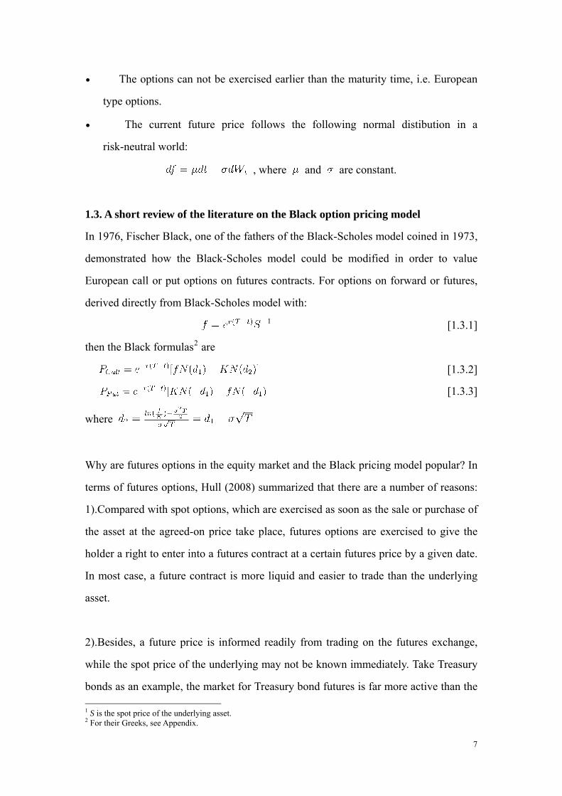
The options can not be exercised earlier than the maturity time, i.e. European
type options.
The current future price follows the following normal distibution in a
risk-neutral world:
, where and are constant.
1.3. A short review of the literature on the Black option pricing model
In 1976, Fischer Black, one of the fathers of the Black-Scholes model coined in 1973,
demonstrated how the Black-Scholes model could be modified in order to value
European call or put options on futures contracts. For options on forward or futures,
derived directly from Black-Scholes model with:
1 [1.3.1]
then the Black formulas2 are
[1.3.2]
[1.3.3]
where
Why are futures options in the equity market and the Black pricing model popular? In
terms of futures options, Hull (2008) summarized that there are a number of reasons:
1).Compared with spot options, which are exercised as soon as the sale or purchase of
the asset at the agreed-on price take place, futures options are exercised to give the
holder a right to enter into a futures contract at a certain futures price by a given date.
In most case, a future contract is more liquid and easier to trade than the underlying
asset.
2).Besides, a future price is informed readily from trading on the futures exchange,
while the spot price of the underlying may not be known immediately. Take Treasury
bonds as an example, the market for Treasury bond futures is far more active than the
1 S is the spot price of the underlying asset. 2 For their Greeks, see Appendix.
7

one for any Treasury bond. The current market price of a bond can not be available
but contacting dealers, whereas a bond futures price is obtained shortly from trading
on the Chicago Board of Trade.
3).One of beauties of a future option for most capitalists is that exercising it does not,
more often than not, result in delivery of the underlying asset, since the underlying
futures contract is closed out prior to delivery commonly. They are eventually settled
in cash.
4).Another advantage for futures options is that they are traded in the same exchange
and facilitates speculation hedging and arbitrage and tends to require lower
transaction costs than spot options to make the markets more efficient.
Traders prefer to Black pricing model to price not only European options on physical
commodities, forward or futures, but also interest rates derivative instruments,
including bond options, interest rate caps and floors and swaptions primarily. They are
widely used to either speculate on the future course of interest rates or to hedge the
interest payments or receipts on an underlying position. Besides, they allow an
investor to benefit from changes in interest rates while limiting any downside losses.
For instance, Black’s model can be used to imply a term structure of forward rates
from actively traded index option.
1.4. Problem formulation
Therefore, it has become a hot issue in the study of pricing interest rate derivatives
like interest rate cap & floors, options of Forward Rate Agreement or European
swaptions. The Black model, alternatively referred as the Black-76 model, is available
as the standard model for valuing these over-the-counter interest rate options. This
model is classified into a class of models known as log-normal forward models under
the assumption that the underlying asset, i.e. the interest rate, is lognormal distributed.
Unfortunately, in the current interest rate market situation with very low or even
8

negative interest rates, different from that of the equity market, the parameter of strike
price (and/or the forward rate (“the price” )can take zero or negative values which
makes a log-normal model hardly take effect and give accurate market prices.
To handle this puzzle, a normal distributed Black model is required. As a matter of
fact, this case was initially considered by Bachelier’s model illustrated as below [1.4.1]
of arithmetic Brownian motion in 1900, it came to be was regarded as an instructive
dead end though. The main reason is that it took time value of money (i.e. lack of the
discount factor) out of consideration. Nonetheless, I suggest here that it is premature
to conclude that an option pricing model with a normal underlying is of no use. In
addition to the work of Bachelier (1990), I would like to mention papers with
introduction related to the research questions by Hagan and Woodward (1998),
Iwasawa (2001), Henrard (2005), Blake, Dawson and Dowd (2007), Grunspan (2011),
together with Benhamou and Nodelman (2013).
[1.4.1]
Accordingly, this brings us to the problems of the paper: when the interest rate is
modeled with a normal distributed stochastic process, what does the model look like?
Do the two models give the identical price with the right volatility? Will the risk, i.e.
the Greeks (delta, gamma, vega, theta and rho), differ when we are shifting the yield
curve? Then the interest rate volatility is normal while in Black the volatility is
log-normal. Both models are supposed to give the same prices and there exists
formula to convert from normal to log-normal or vice verse. Therefore, in a trading
point of view and from a risk perspective, a study of a normal and a log-normal Black
model is of great interest.
For this paper, the author describes the current state of the interest rate derivatives
market in the context of normal distributed Black options pricing model against
classical Black model. The theory depends upon various areas of applied mathematics
9

with specialization in financial engineering, including stochastic calculus, the
implementation of a dynamic hedging strategy, the notable no-arbitrage argument, the
application of Feynman-Kač, the equivalent martingale measure and particularly risk
measures. Also singular perturbation theory explains how one can approximate
normal volatility with log-normal one. The paper unifies couples of results scattered
throughout the mathematical and financial literature and papers, as well as it tests
empirically new outcomes from this highly promising area by the author, with the
assistance of Excel VBA.
2. Derivation of equation and formulas
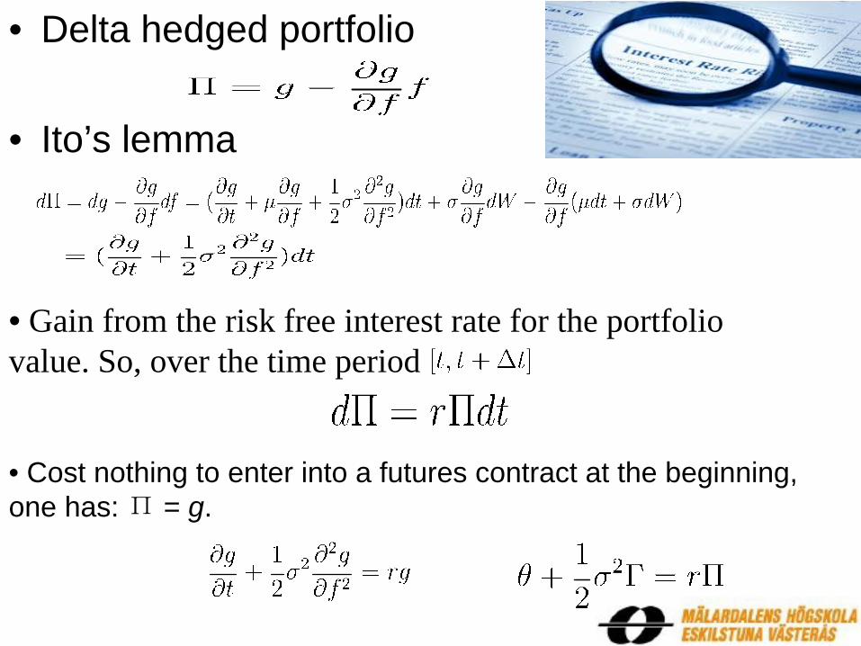
Start by constructing a certain portfolio, called the delta hedged portfolio, consisting
of being long delta shares of future contract and short one derivative in question. Say,
call it Π. Let us also denote the value of derivative by g. Then, the value of the
delta-hedged portfolio is given by:
[2.1]
So applying Ito’s lemma using the SDE given above into the changes of the portfolio
value, one gets:
[2.2]
Notice that the term has vanished. Thus uncertainty has been eliminated and the
portfolio is effectively riskless. The rate of return on this portfolio must be equal to
the rate of return on any other riskless instrument; otherwise, there would be
opportunities for arbitrage. We want the above riskless portfolio to be a martingale
under the discounted expectation. This is to say that the above quantity equals the
gain from the risk free interest rate for the portfolio value. So, over the time
period we have:
[2.3]
10

Since it cost nothing to enter into a futures contract at the beginning, one has: Π = g.
Thus, we arrive at the following partial differential equation:
[2.4]
To test the effectiveness of this strategy, simulate the returns to dealers with short
positions in payer and receiver swaptions respectively who perform daily rehedging
over the lifetime of the swaptions. Monte Carlo simulation is available to model the
evolution of the underlying forward swap price, assuming a normal distribution. It is
assumed that a dealer starts with zero cash and borrowing or depositing at the riskless
interest rate in response to the cashflows gained by the dynamic hedging strategy.
As Merton (1973) and Blake, Dawson and Dowd (2007) indicate, since the portfolio
requires zero investment, it must be that to avoid “arbitrage” profits, the expected and
realized return on the portfolio with this strategy is zero. Merton’s model was
predicated on rehedging in continuous time, which would bring about expected and
realized returns being identical. In practice, traders tend to use discrete time rehedging
alternatively. One outcome of this is that, over a large number of simulations, the
expected return will be zero, although on any individual simulation, the realized
return may differ from zero.
In a risk neutral world, the process followed by the variable V known as a Wiener
process is giving as with the trivial solution, from integration over the
interval [t, T]:
[2.5]
As far as we can see , since has a standardized normal distribution with mean 0 and
variance 1, then is a Gaussian process; , i.e. with mean and
variance . According to the above parabolic partial differential equation
[2.4], the terminal payoff is .By the application of Feynman-Kač to
11

compute the expectations of random process equivalent to the integral of a solution to
a diffusion equation, we obtain the following solution:
[2.6]
where 3
Intuitively, couple [2.5] with [2.6] and the solution can also be expressed as:
[2.7]
Therefore, the formula for the above can be simplified by simply expanding the
expression inside the integral. The detail will be shown for more general audience.
For the call, we have:
[2.8]
Set and with we get
3 refers to ; Similarly, refers to .
12
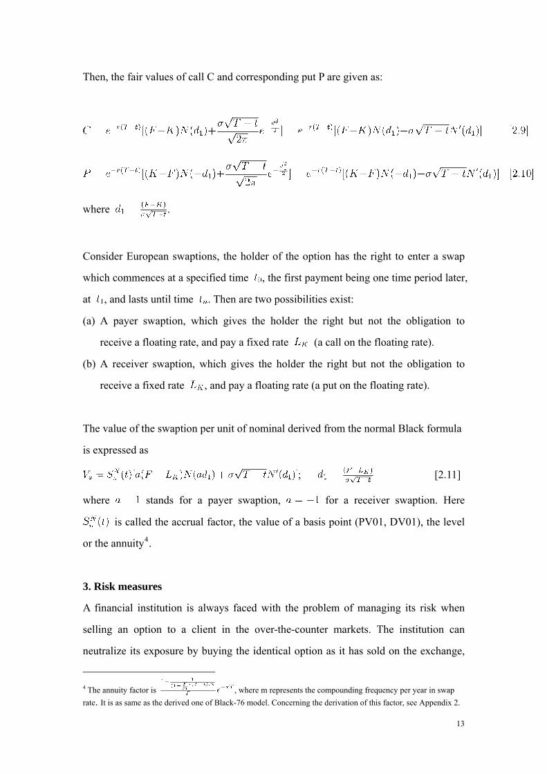
Then, the fair values of call C and corresponding put P are given as:
where .
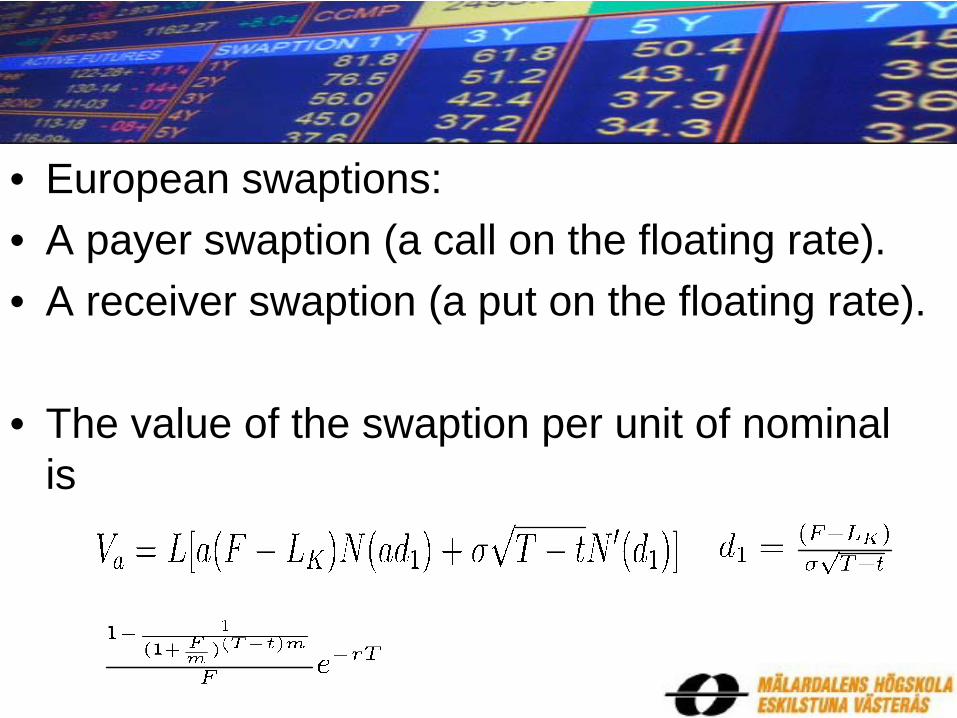
Consider European swaptions, the holder of the option has the right to enter a swap
which commences at a specified time , the first payment being one time period later,
at , and lasts until time . Then are two possibilities exist:
(a) A payer swaption, which gives the holder the right but not the obligation to
receive a floating rate, and pay a fixed rate (a call on the floating rate).
(b) A receiver swaption, which gives the holder the right but not the obligation to
receive a fixed rate , and pay a floating rate (a put on the floating rate).
The value of the swaption per unit of nominal derived from the normal Black formula
is expressed as
; [2.11]
where stands for a payer swaption, for a receiver swaption. Here
is called the accrual factor, the value of a basis point (PV01, DV01), the level
or the annuity4.
3. Risk measures
A financial institution is always faced with the problem of managing its risk when
selling an option to a client in the over-the-counter markets. The institution can
neutralize its exposure by buying the identical option as it has sold on the exchange,
4 The annuity factor is , where m represents the compounding frequency per year in swap
rate. It is as same as the derived one of Black-76 model. Concerning the derivation of this factor, see Appendix 2.
13

as long as the option happens to be the same as one that is traded on an exchange.
However, when the option has been customized to the demands of a client and does
not correspond to the standardized products traded by exchanges, then hedging the
exposure is much trickier.
To solve this, alternative approaches are commonly referred to as the ‘Greeks’. The
Greeks are vital tools in risk management. Each Greek letter measures the risk in a
different dimension in an option position and the purpose of a trader is to manage the
Greeks so that all risks are acceptable enough. Limits are defined for each Greek letter.
For example, the delta limit is often expressed as the equivalent maximum position in
the underlying asset. Besides, the vega limit is usually expressed as a maximum dollar
exposure per 1% change in the volatility. And special permission is necessary if a
trader intends to exceed a limit at the end of a trading day. Moreover, the first-order
Greeks (delta, gamma, vega, theta and rho) are computed by simple differentiation of
the above formulas, as exhibited below one by one in this section.
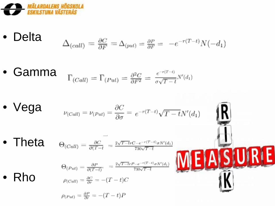
3.1. Delta
Most importantly, the delta of an option is the rate of change of its price with
respect to the price of the underlying asset. According to the put–call parity, a long
call plus a short put (a call minus a put) replicates a forward, which has delta equal to
1. That is, for a European call and put option for the same strike price and time to
maturity of underlying, and without dividend yield, the sum of the absolute values of
the delta of each option will be 1.00.
Since the delta of underlying asset is always 1.0, the trader could delta-hedge his
entire position in the underlying by buying or shorting the number of shares indicated
by the total delta. For example, if the delta of a portfolio of options in Z (expressed as
shares of the underlying) is +1.75, the trader would be able to delta-hedge the
portfolio by selling short 1.75 shares of the underlying. This portfolio will then keep
its total value whichever direction the price of Z moves. The delta of an option varies
14

over time, thus the position in the underlying asset has to be rebalanced by traders at
least on a daily basis.
[3.1]
[3.2]
In the equity market, delta is trivial since an underlying instrument can vary in price.
Nevertheless, in the context of interest rate theory, the changes occur as a change in
the interest rate curve. Not a single value (point), but the whole curve. This implies
that delta risk is the risk associated with a shift in the zero curve. Thus, delta can be
defined in several alternatives:
i) By shifting the swap rate (F), i.e., the fixed rate in an underlying swap. It is the
standard in some trading systems to take the analytical derivative of the
swaption price with respect to the forward swap rate, ignoring the annuity
term which also depends on the swap rate via the discount factors.
ii) By shifting the yield curve (the zero coupon curve) with one basis-point (1bp
= 0.01 %). This is sometimes termed as DV01 or PV015. This approach
assumes implicitly a parallel evolution of the interest rate curve.
iii) By shifting the quoted rate, before bootstrapping the market quotes to a zero
curve. Traders argue that the zero curve can changes only if the quote for the
instruments used to calculate the zero curve changes. In this delta definition,
one computes as many as deltas as there are market instruments. Each delta
corresponds to the isolated influence of the change of the market quote of one
5 PV01 is the variation in ‘‘Present Value’’ of a 1 basis-point shift of the rate; DV01 refers to the same ratio expressed in “Dollar”. They are analogous to the delta in derivative pricing and almost the same.
15
market instrument. Thus it makes sense to outline the exposures arising from
the changes in the quote.
iv) By calculating the change in the value of the swaption with respect to the
change of the underlying swap value when making a shift in the curve as ii) or
iii).
v) By shifting of certain section or time buckets of the interest rate curve. The
risk profile is aggregated, as bucket delta measures the impact of shifting the
rates of a given bucket by one basis point while the other buckets stay
unchanged. The fair forward swap rate is dependent upon the bootstrap and
interpolation method associated with the construction of the yield curve. When
applying continuous compounding of the interest rate mathematically to
express the forward rate, the yield on all maturities can change by the same
number of basis points and a parallel shift in the yield curve occurs.
Unfortunately, the world is far from that simple because the zero rates can tilt
up or down over a long term and the risk is placed unevenly in time buckets.
As a result, a change in the yield curve with different maturities in which the
changes in yields do not occur evenly in the financial market. This method is
quite useful to give a condensed overview of the risk when the traders intend
to hedge partially risks.
3.2. Gamma
Once an option position has been made delta neutral, the next step is to focus on its
gamma .It is the rate of change of its delta with respect to the price of the
underlying asset. It is a measure of the curvature of the relationship between the
option price and the asset price. The impact of this curvature on the performance of
delta hedging can be decreased by making an option position gamma neutral. To be
more exactly, if is the gamma of the position being hedged, this decrease is often
completed by taking a position in a traded option that has a gamma of . It is
16

evident from the Put-Call parity that by differentiating the put and call formula twice
with respect to the underlier establishes the equality of gamma of put and call for
option models.
[3.3]
3.3. Vega
Practically, volatilities of the underlying asset are stochastic throughout the time,
while delta and gamma hedging are under the assumption that the volatility remains
constant. The vega of an option or an option portfolio measures the rate of change
of its value with respect to volatility. Vega can be an important Greek to monitor for
an option trader, especially in volatile markets. Making the position vega neutral can
help trader hedge an option position against volatility changes. Again, from the
Put-Call parity, by differentiating the put and call formula twice with respect to
comes to the equality of put and call for option models.
[3.4]
Put-Call Parity:
Since vega is conventionally presented by practitioners in terms of a one percentage
point change in volatility, then vega can also be . To create both
gamma and vega neutrality, two traded derivatives dependent on the underlying asset
must be used. Unlike delta, typically it is far from feasible to maintain gamma and
vega neutrality regularly. If they get too large, trading is curtailed or corrective action
17

is taken.
3.4. Theta and Rho
Another measure of the risk of an option position is theta which measures the rate
of change of the value of the position with respect to the passage of time, with the rest
holding constant. As demonstrated below, the chain rule and the product rule as well
as the sum rule are applied implicitly. By convention, practitioners quote theta as the
change in an option’s value as one day passes, as exhibited [3.5B]&[3.6B]. On top of
those, to measure the rate of change of the value of the position with respect to the
interest rate, rho is available. The value of an option is generally less sensitive to
changes in the risk free interest rate than to changes in other parameters. For this
reason, rho is the least used of the first-order Greeks.
[3.5A]
[3.5B]
[3.6A]
18

[3.6B]
[3.7]
[3.8]
It has been proved previously that the price of a single derivative dependent on a
future contract must satisfy the differential equation [2.4]. It follows that the value of
of a portfolio of such derivatives also satisfies the differential equation
. [3.9]
Since
,
then it follows that
. [3.10]
4. Equivalence between the normal and the lognormal implied volatility
In the real market, it is standard practice to quote the swaptions in term of log-normal
volatility (Black volatility) which is inserted into the Black model to find the price.
Meanwhile, normalized volatility is also the market convention though, primarily
because normalized volatility deals with basis point changes in rates rather than, as in
lognormal volatility, with percentage changes in rates. Therefore one needs to
calculate the implied normal volatility.
In this derived model, the interest rate is modeled with a normal distributed stochastic
process. Then the interest rate volatility is normal while the volatility is log-normal in
Black-76 model. Both models are supposed to give the same prices and there exist
formula to convert from normal to log-normal or log-normal to normal. Such formula
can be derived with the help of perturbation theory which is applicable if the problem
at hand can be formulated by adding a "small" term to the mathematical description of
19

the exactly solvable problem.
4.1 Singular perturbation expansion
Consider a European call with expiration date , settlement date , and strike K. As
before, let be the stochastic process for the forward price as seen at date with
‘‘adjustment’’. We are assuming that
[4.1]
under the forward measure. Under this measure, the value of the option at date is
, where the function is given by the expected value
[4.2]
Here is the discount factor to the settlement date at date .
By using singular perturbation methods to solve the scaled problem, we analyze
Black’s model to determine the volatility which would yield the same value of
the option. As Hagan and Woodward (1998) proved previously, the value of the call
option is
, [4.3]
where
Lastly, the equivalent Black volatility implied by this price is computed as below:
Where [4.4]
To yield the more precise equivalent volatility formula, arbitrarily high order can be
performed via . A similar analysis shows that the implied volatility for a
European put option is given by the same formula.
20

4.2 Conversion between log normal and normal volatility
Black’s model is where is present forward swap (or
caplet) rate and is the implied log normal volatility, while the normal model is
, where is the normal volatility. To translate from normal
to lognormal vol., the formula proved earlier by Hagan(1998) and Viorel and Dan
(2011) is
[4.5]
as
Alternatively, considering some terms are too small to affect its precision, the formula
could be simplified as below:
[4.6]
when With these formulas and the normal volatility, then make use of
a global Newton method to find log-normal one approximately.
5. Empirical test on disparities between Black model and normal Black model
In this section, to take a close graphical look at how the risks for a swaption differ
between the log-normal Black model and normal one, some empirical tests are
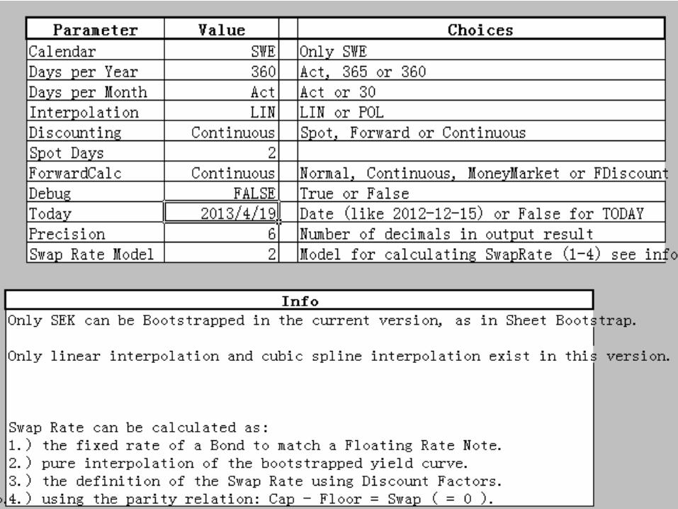
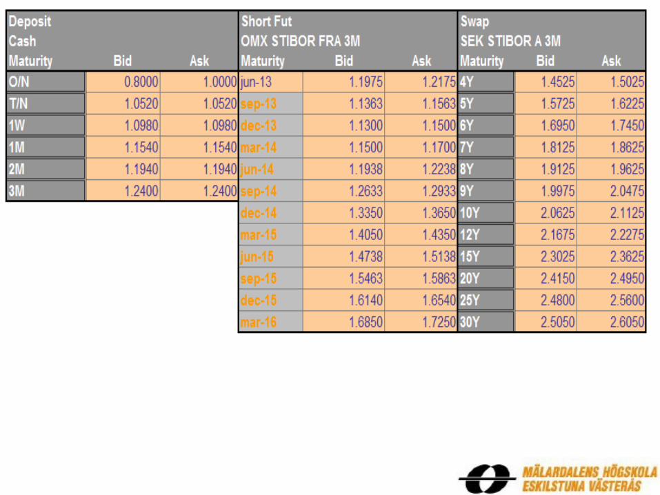
performed by the Excel VBA.6 Starting from the setup, the values of parameters are
defined specifically. Only Swedish calendar is valid to bootstrap, as well as 360 days
per year actual days per month. The beginning date is 2013/4/19. The rates quoted in
the market are par yields from which the zero coupon rate is derived. To bootstrap a
zero-coupon curve, there are liquid instruments on the Swedish market, i.e. an
over-night rate (O/N), a tomorrow-next rate (T/N), deposit rates for one week, one,
two and three month maturities, some OMX STIBOR Forward Rate Agreements
6 This VBA application was programmed originally by Jan Röman. See the demo of input-output interfaces in the Appendix.
21
(FRA) and finally swaps from 4 year up to 30 year. Swap rate is calculated as pure
interpolation of the bootstrapped yield curve. For the years when there is shortage of
swap rates, use the linear extrapolation to find the zero rates and then in the same way
to calculate the discount factors as well as forward rate in turn.
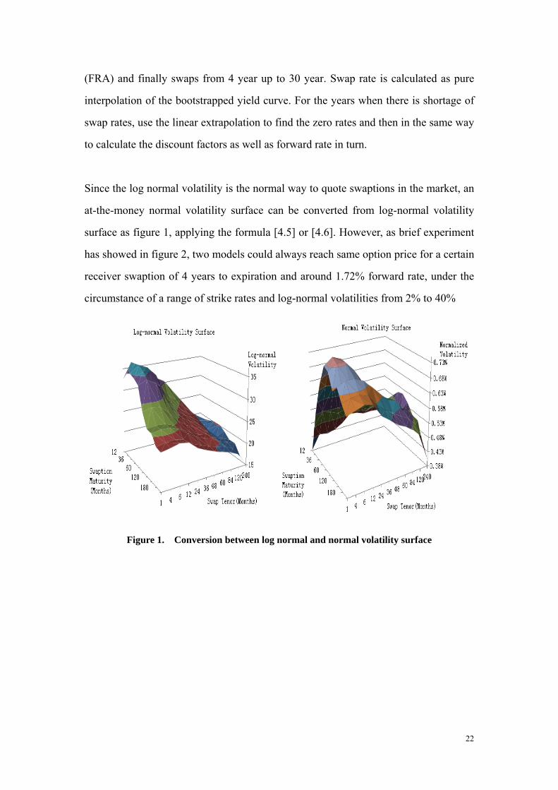
Since the log normal volatility is the normal way to quote swaptions in the market, an
at-the-money normal volatility surface can be converted from log-normal volatility
surface as figure 1, applying the formula [4.5] or [4.6]. However, as brief experiment
has showed in figure 2, two models could always reach same option price for a certain
receiver swaption of 4 years to expiration and around 1.72% forward rate, under the
circumstance of a range of strike rates and log-normal volatilities from 2% to 40%
Figure 1. Conversion between log normal and normal volatility surface
22

Figure 2. Approximation experiments on receiver Swaption price surface with Black model
and normal Black model
In terms of delta and vega, their disparities between models are also of significance.
On one hand, when the forward rate is identical to strike rate and the log-normal
volatility increases, its vega decreases and its delta rises, while the curves of their
normal counterparties hovers, exhibited as figure 3. On the other hand, if the forward
rate differs from the strike rate, the difference between log-normal delta and normal
one accelerates with respect to the growing volatility; whereas the gap between
log-normal vega and normal vega tend to not only go up majorly but move down to
zero somewhere by all means, as demonstrated in figure 4&5.
Figure 3. Disparity between the Black Vega(Delta) and normal Vega(Delta) with respect to
Black volatility when forward rate is as same as strike rate (At the Money)
23
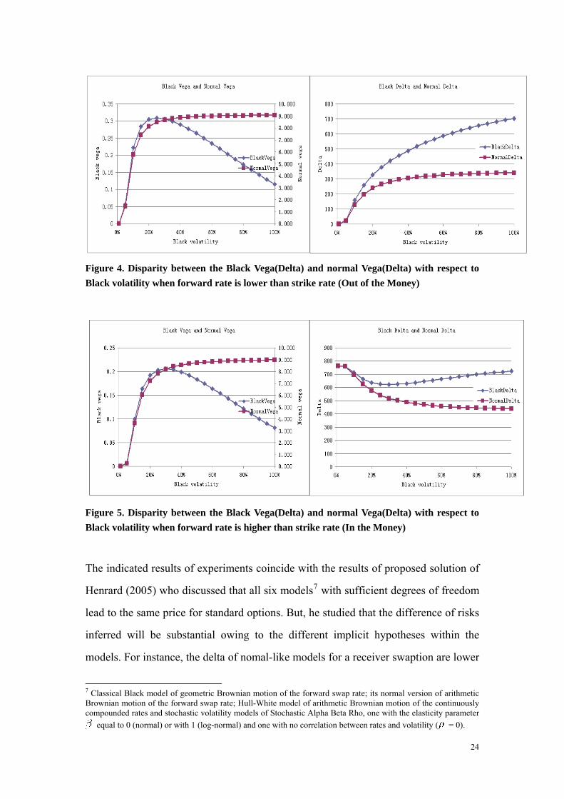
Figure 4. Disparity between the Black Vega(Delta) and normal Vega(Delta) with respect to
Black volatility when forward rate is lower than strike rate (Out of the Money)
Figure 5. Disparity between the Black Vega(Delta) and normal Vega(Delta) with respect to
Black volatility when forward rate is higher than strike rate (In the Money)
The indicated results of experiments coincide with the results of proposed solution of
Henrard (2005) who discussed that all six models7 with sufficient degrees of freedom
lead to the same price for standard options. But, he studied that the difference of risks
inferred will be substantial owing to the different implicit hypotheses within the
models. For instance, the delta of nomal-like models for a receiver swaption are lower
7 Classical Black model of geometric Brownian motion of the forward swap rate; its normal version of arithmetic Brownian motion of the forward swap rate; Hull-White model of arithmetic Brownian motion of the continuously compounded rates and stochastic volatility models of Stochastic Alpha Beta Rho, one with the elasticity parameter
equal to 0 (normal) or with 1 (log-normal) and one with no correlation between rates and volatility ( = 0).
24

than that of log-normal-like Black models. The difference in the delta can reach 10%
or more of the underlying even if models are calibrated to the identical prices.
Therefore, it is convincible enough to ensure that the above investigated analysis
holds strongly.
6.Conclusion
Ever since it became clear that a geometric Brownian motion process provides a more
plausible model of asset prices than an arithmetic Brownian motion process, it has
been taken for granted that there was no point in developing an option pricing model
for a normally distributed underlying. Nonetheless, it has been argued that there are
potential in which we might need such a model when the forward rate is zero and/or
when the strike rate is equal zero or negative, and a contemporary example is when
the interest rate is negative.
In the second section, the derivation of the model is subject to the assumption that
implementation of a dynamic hedging strategy will eliminate the risk of holding long
or short positions in such options. Additionally, the derivation of the formulas has
been proved mathematically by the famous no-arbitrage argument. The idea of the
theory is that the fair value of any derivative security is computed as the expectation
of the payoff under an equivalent martingale measure. In the section 3, the Greeks
have been derived analytically by differentiation. Also brief explanation regarding
how one can approximate log-normal Black with normal version has been explored in
the fourth section. Eventually, there is an empirical test for swaptions on an
at-the-money volatility surface, given as Black (log-normal) volatilities, which is
converted to a normal volatility surface. Then calculate and plot how delta and vega
differs between the models.
Admittedly, both models have limitations in routine pricing and do not provide a
description of how interest rates evolve through time, concerning pricing interest rate
derivatives such as American style swap options. Interest rate derivatives are tougher
25

to value than equity and foreign exchange derivative due to the complicated behavior
of an individual interest rate and the varying volatilities of different points on the
yield curve. As a matter of fact, other notable models, like Hull-White model, can be
calibrated to the market as well. I believe that either model can be valuable in my
future study.
To sum up, the crucial risk sensitivities for such fixed income derivatives as swaptions
are delta (PV01, DV01) and Vega among Geeks, as a result of their risk limits set by
the trading desk. Thanks to the conversion formula between log-normal volatility and
normal volatility, it has been found in this paper that both models results in same
option value despite of the disparities in their risks. Accordingly, an option-pricing
model based on a normal underlying is not some flawed relative of Black, as it is
usually considered to be, but is instead the key to correctly pricing this type of
derivatives– and hence, from a risk perspective as well as in a trading point of view, a
very helpful tool in the rapidly emerging interest rate derivatives market.
26
7. Reference
Bachelier, L., (1900) ,Théorie de la Spéculation., Paris: Gauthier-Villars
Benhamou, E. and S. Nodelman, (2013), Delta Risk on Interest Rate Derivatives,
London FICC, Goldman Sachs International
Black, F., and M. Scholes, (1973), The Pricing of Options and Corporate Liabilities,
Journal of Political Economy. 81:637-654
Blake, D., Dawson, P., and K. Dowd, (2007), Options on Normal Underlyings,
Nottingham University Business School
Downes, J. and J. Goodman, (2010), Dictionary of Finance and Investment Terms, 8th
edition, published by Barron's Educational Series Inc
Grunspan, C., (2011), A Note on the Equivalence between the Normal and the
Lognormal Implied Volatility: A Model Free Approach, Department of Financial
Engineering, ESLV, Paris
Hagan, P., Volatility Conversion Calculators, Bloomberg
Hagan, P. and D. Woodward, (1998), Equivalent Black Volatilities ,March 30,1998,
The bank of Tokyo-Mitsubishi
Henrard, M., (2005), Swaptions:1 Price, 10 Deltas, And … 6 1/2Gammas, Derivatives
Group, Banking Department, Bank for International Settlements, Basel Switzerland
Hull, J., (2008), Options, Futures and Other Derivatives, 7th edition, Pearson Prentice
Hall
27

28
Karatzas, I., and S.E. Shreve, (1988), Brownian Motion and Stochastic Calculus,
Springer-Verlag, New York
Iwasawa, K., (2001), Analytical Formula for the European Normal Black Scholes
Formula, Department of Mathematics, New York University
Merton, C., (1973), Theory of Rational Option Pricing, Bell Journal of Economics
and Management Science. 4: P141 – 183.
Röman, J., (2012), Lecture Notes in Analytical Finance II, Department of
Mathematics and Physics, Mälardelen University, Sweden
West, G. and L. West, (2011), Introduction to Black’s Model for Interest Rate
Derivatives, Financial Modelling Agency Inc, South Africa
Remarks concerned the use of Internet, correctness of citations:
I certify that I have checked the correctness of citations in this thesis, and I did not
copy material from any Internet Web page, but used the Internet preprint. The data in
the Excel are taken by Jan Röman from one of trading system at Swedbank, Murex ,
Mx3.

Appendix
Table 1: Risk measures for the Black model
Greeks Call Put
Delta
Gamma
Vega
Theta
Rho

2. Black formulas expressed for Caps/Floors and Swaptions & annuity factor
The Black formula for the time-t value of a caplet and a floorlet are expressed as:
Where is the tenor, the face value and F the implied forward rate between time
t and at the caplets/floorlets maturity, T.
From Black model, a payer swaption and a receiver swaption are expressed as :
where T-t = Tenor of swap in years (time between swaption maturity and swap maturity). F = Forward rate of the underlying swap. K = Strike rate of the swaption. r = Risk-free interest rate. T = Time to swaption expiration in years.
= Volatility of the forward-starting swap rate.
m = Compounding’s per year in swap rate.
Derivation of annuity factor of swaptions8
To derive the factor for a swaption, start by studying a forward starting swap. That is a swap that starts at a future time where we exchange floating for fixed cash flows. A
swap means a swap that start at time and have maturity at time .
Define the reset days for any swap as: and denote as The holder of a forward starting payer swap with tenor receives fixed payments at times and pay at the same times floating payments. For each period , the LIBOR rate is set at time and the floating leg is received at . For the same period the fixed leg is
8 Röman, J., (2012), Lecture Notes in Analytical Finance II, Mälardelen University, p370-373.

paid at where F is the (fixed) swap rate.
The non-arbitrage value at of the floating payment made at is given by . The total value of the floating legs at time t for equals
where the forward rate is given by:
The value at the starting day is the same as the face value = 1. In a swap, there is not any final payment of the face value. This gives the swap value at the starting day t = 0, as 1 – p(0, T). Between to resets therefore must the swap value must be as:
where is the time for the next reset day. This explains the formula above. The total value at time t for the fixed side equals
where F is called the swap rate. This is a par rate since it makes the price of the swap to be equal zero when entering the swap contract. So the total value of the payer swap is given by
Thus define the forward swap rate (at par) of the swap as the value of F for which the total value above is zero. I.e.,
In addition, define for each pair n, k with n < k, the process
as the accrual factor or the value of a basis point (also called the level, DV01, PV0l, annuity or numerical duration of the swap). Then express the swap value as:
In the market there are no quoted prices for different swaps. Instead there are market quotes for the par swap rates. Calculate the arbitrage free price for a payer swap with
31

the strike rate K as
A payer swaption is then a contract given by:
This contract gives the holder the right to enter a swap contract at time with swaption strike (fixed rate) K. Under the numeraire process a payer swaption is then a call option on with strike\ price K. The value of this contract is given by the Black-76 formula:
The Black formula can be written as:
If denote the Forward swap-rate between and as F, at it is:
Now let be the maturity of the swaption, F the Forward swap-rate above) and introducing m reset days per year (the frequency).
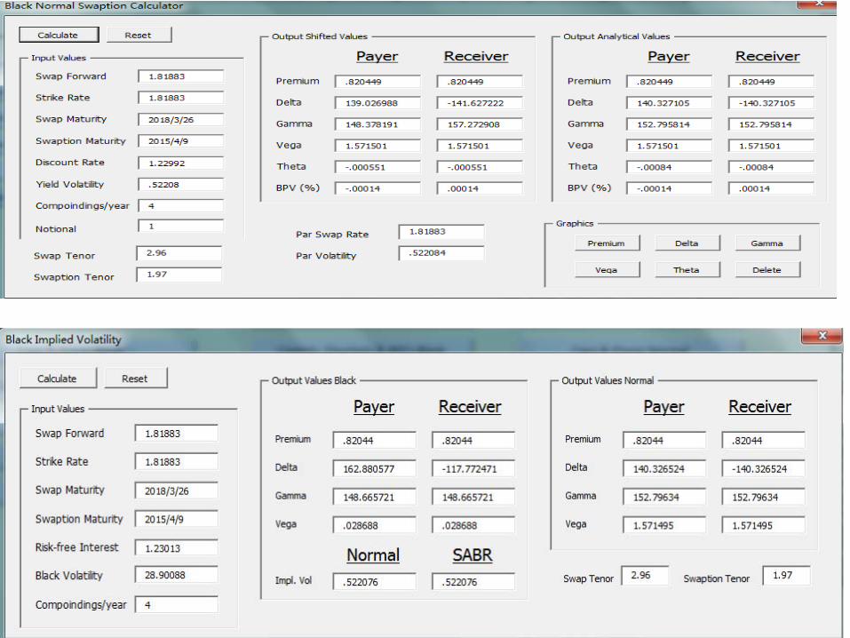
3. Presentation of input-output interfaces
Figure 6. Demo of classical Black and normal Black swaption calculator given Black implied
volatility
32

Figure 7. Demo of Black normal swaption calculator
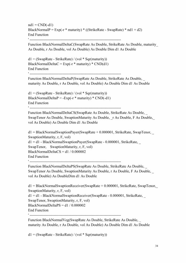
4. Extract of VBA program codes
' Base function for the normal Black model (C = Call, P = Put options) 'For all functions below, the following is used. ' The SwapRate, StrikeRate, r and vol is given in %. I.e., 3.4 % as 0.034 ' The SwapTenor and SwaptionMaturity are given in years. ' F is the frequency, i.e., the mumber of cash-flows per year ' N (the face value, notional) is not used (use this outside this function) ' ===================================================== Function Annuity(SwapRate As Double, Tenor As Double, F As Double) As Double Annuity = (1 - 1 / Pow(1 + SwapRate / F, F * Tenor)) / SwapRate End Function ' ------------------------------------------------------------------------- Function BlackNormalC(SwapRate As Double, StrikeRate As Double, maturity As_ Double, r As Double, vol As Double) As Double Dim d1 As Double, d2 As Double,_ nd1 As Double d1 = (SwapRate - StrikeRate) / (vol * Sqr(maturity)) d2 = vol * Sqr(maturity / (2 * 3.141592654)) * Exp(-d1 * d1 / 2) nd1 = CND(d1) BlackNormalC = Exp(-r * maturity) * ((SwapRate - StrikeRate) * nd1 + d2) End Function ' ------------------------------------------------------------------------- Function BlackNormalP(SwapRate As Double, StrikeRate As Double, maturity As_ Double, r As Double, vol As Double) As Double Dim d1 As Double, d2 As Double,_ nd1 As Double d1 = (SwapRate - StrikeRate) / (vol * Sqr(maturity)) d2 = vol * Sqr(maturity / (2 * 3.141592654)) * Exp(-d1 * d1 / 2)
33
nd1 = CND(-d1) BlackNormalP = Exp(-r * maturity) * ((StrikeRate - SwapRate) * nd1 + d2) End Function ' ------------------------------------------------------------------------- Function BlackNormalDeltaC(SwapRate As Double, StrikeRate As Double, maturity_ As Double, r As Double, vol As Double) As Double Dim d1 As Double d1 = (SwapRate - StrikeRate) / (vol * Sqr(maturity)) BlackNormalDeltaC = Exp(-r * maturity) * CND(d1) End Function ' ------------------------------------------------------------------------- Function BlackNormalDeltaP(SwapRate As Double, StrikeRate As Double, _ maturity As Double, r As Double, vol As Double) As Double Dim d1 As Double d1 = (SwapRate - StrikeRate) / (vol * Sqr(maturity)) BlackNormalDeltaP = -Exp(-r * maturity) * CND(-d1) End Function ' ------------------------------------------------------------------------- Function BlackNormalDeltaCS(SwapRate As Double, StrikeRate As Double, _ SwapTenor As Double, SwaptionMaturity As Double, _r As Double, F As Double,_ vol As Double) As Double Dim d1 As Double d1 = BlackNormalSwaptionPayer(SwapRate + 0.000001, StrikeRate, SwapTenor, _ SwaptionMaturity, r, F, vol) d1 = d1 - BlackNormalSwaptionPayer(SwapRate - 0.000001, StrikeRate, _ SwapTenor, SwaptionMaturity, r, F, vol) BlackNormalDeltaCS = d1 / 0.000002 End Function ' ------------------------------------------------------------------------- Function BlackNormalDeltaPS(SwapRate As Double, StrikeRate As Double, _ SwapTenor As Double, SwaptionMaturity As Double, r As Double, F As Double, _ vol As Double) As DoubleDim d1 As Double d1 = BlackNormalSwaptionReceiver(SwapRate + 0.000001, StrikeRate, SwapTenor,_ SwaptionMaturity, r, F, vol) d1 = d1 - BlackNormalSwaptionReceiver(SwapRate - 0.000001, StrikeRate, _ SwapTenor, SwaptionMaturity, r, F, vol) BlackNormalDeltaPS = d1 / 0.000002 End Function ' ------------------------------------------------------------------------- Function BlackNormalVeg(SwapRate As Double, StrikeRate As Double, _ maturity As Double, r As Double, vol As Double) As Double Dim d1 As Double d1 = (SwapRate - StrikeRate) / (vol * Sqr(maturity))
34
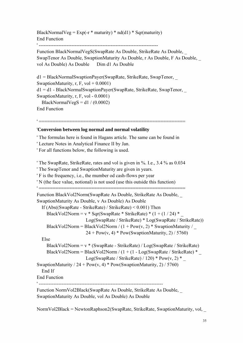
BlackNormalVeg = Exp(-r * maturity) * nd(d1) * Sqr(maturity) End Function ' ------------------------------------------------------------------------- Function BlackNormalVegS(SwapRate As Double, StrikeRate As Double, _ SwapTenor As Double, SwaptionMaturity As Double, r As Double, F As Double, _ vol As Double) As Double Dim d1 As Double d1 = BlackNormalSwaptionPayer(SwapRate, StrikeRate, SwapTenor, _ SwaptionMaturity, r, F, vol + 0.0001) d1 = d1 - BlackNormalSwaptionPayer(SwapRate, StrikeRate, SwapTenor, _ SwaptionMaturity, r, F, vol - 0.0001) BlackNormalVegS = d1 / (0.0002) End Function ' =====================================================
'Conversion between log normal and normal volatility
' The formulas here is found in Hagans article. The same can be found in ' Lecture Notes in Analytical Finance II by Jan. ' For all functions below, the following is used. ' The SwapRate, StrikeRate, rates and vol is given in %. I.e., 3.4 % as 0.034 ' The SwapTenor and SwaptionMaturity are given in years. ' F is the frequency, i.e., the mumber od cash-flows per year ' N (the face value, notional) is not used (use this outside this function) ' ===================================================== Function BlackVol2Norm(SwapRate As Double, StrikeRate As Double, _ SwaptionMaturity As Double, v As Double) As Double If (Abs((SwapRate - StrikeRate) / StrikeRate) < 0.001) Then BlackVol2Norm = v * Sqr(SwapRate * StrikeRate) * (1 + (1 / 24) * _ Log(SwapRate / StrikeRate) * Log(SwapRate / StrikeRate)) BlackVol2Norm = BlackVol2Norm / (1 + Pow(v, 2) * SwaptionMaturity / _ 24 + Pow(v, 4) * Pow(SwaptionMaturity, 2) / 5760) Else BlackVol2Norm = v * (SwapRate - StrikeRate) / Log(SwapRate / StrikeRate) BlackVol2Norm = BlackVol2Norm / (1 + (1 - Log(SwapRate / StrikeRate) * _ Log(SwapRate / StrikeRate) / 120) * Pow(v, 2) * _ SwaptionMaturity / 24 + Pow(v, 4) * Pow(SwaptionMaturity, 2) / 5760) End If End Function ' ---------------------------------------------------------------------------- Function NormVol2Black(SwapRate As Double, StrikeRate As Double, _ SwaptionMaturity As Double, vol As Double) As Double NormVol2Black = NewtonRaphson2(SwapRate, StrikeRate, SwaptionMaturity, vol, _
35

2 * vol / (SwapRate + StrikeRate)) End Function ' ---------------------------------------------------------------------------- Function NewtonRaphson2(SwapRate As Double, StrikeRate As Double, _ SwaptionMaturity As Double, cm As Double, Optional initial As Double) As Double Dim dVol As Double Dim EPSILON As Double Dim maxIter As Double Dim vol_1 As Double Dim vol_2 As Double Dim vol_3 As Double Dim old_err As Double Dim i As Double Dim dX As Double Dim Value_1 As Double Dim Value_2 As Double dVol = 0.00001 EPSILON = 0.00001 maxIter = 100 vol_1 = initial i = 1 old_err = 9E+99 Do Value_1 = BlackVol2Norm(SwapRate, StrikeRate, SwaptionMaturity, vol_1) vol_2 = vol_1 - dVol Value_2 = BlackVol2Norm(SwapRate, StrikeRate, SwaptionMaturity, vol_2) dX = (Value_2 - Value_1) / dVol If Abs(old_err) < EPSILON Or i > maxIter Or dX = 0 Then Exit Do old_err = -(cm - Value_1) / dX vol_1 = vol_1 - (cm - Value_1) / dX Debug.Print vol_1 i = i + 1 Loop Debug.Print vol_1 NewtonRaphson2 = vol_1 End Function ' ----------------------------------------------------------------------------
5. Summary of reflection of objectives in the thesis
Objective 1.
Survey of literature with comments related to the current research questions:
Second paragraph of section 1.4.
36

37
Survey and comparison of alternative methods related to the subject of the
project: Section 3.1
Deeper presentation of specific methods supposed to be used in the project:
Section 2, 3, 4, 5.
Objective 2.
Description of the model and comparisons with alternative models: Section1.3
Analysis of data, their quality, volume, shortage, etc. (if any): First
paragraph of section 5
Objective 3.
Formulation of the problem studied in the project and the goals of the project:
Section 1.4
Evaluation of possible solution in the time framework and presentation of
solution (algorithms, results of experiments, description of programs,
presentation of input-output interfaces, etc): Section 5, Appendix 3. The
algorithms are based on the formulas of section 3,4.
Program codes: Appendix 4
Objective 4.
Print of the oral presentation of the project. PowerPoint
Improved English and the thesis structure (abstract, table of contents, sections,
conclusion, references). Everywhere
The place of results in the area; the list of main results and achievements;
potential use of results; possible future continuation of the project: Section 6.
Objective 6.
Popular presentation of project and its results: Last paragraph of Section 1.4.
Remarks concerned the use of Internet and correctness of citations: In the end
of section 7.
Acknowledgement: Page 2
Risk Measures with Normal Distributed Black Options Pricing Model
WenqingWenqing
HuangHuang
Supervised by AnatoliyAnatoliy MalyarenkoMalyarenko & Jan & Jan RRöömanman
Bachelor Degree Project in Financial Mathematics

Contents•• 1.Introduction1.Introduction• 1.1. Negative interest rates• 1.2. The notations and assumptions• 1.3. A short review of the literature on the Black option pricing model• 1.3. Problem formulation
•• 2. Derivation of equation and formulas2. Derivation of equation and formulas
•• 3. Risk measures3. Risk measures
•• 4. Equivalence between the normal and the lognormal implied vola4. Equivalence between the normal and the lognormal implied volatilitytility• 4.1 Singular perturbation expansion• 4.2 Conversion between log normal and normal volatility
•• 5. Empirical test on disparities between Black model and normal 5. Empirical test on disparities between Black model and normal Black Black modelmodel
•• 6.Conclusion6.Conclusion•• AppendixAppendix
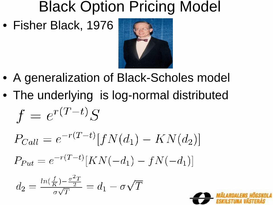
Black Option Pricing Model• Fisher Black, 1976
• A generalization of Black-Scholes model
• The underlying is log-normal distributed

• Equity market
• Interest rate derivatives market
Bond options
Caps and floors
Swaptions
FRA
…
• Future option VS Spot one
• More liquid , price known readliy, settle in cash, lower cost

Negative Interest Rate
• Macroeconomics
Japan, in 1990s
Sweden’s Riksbank,-0.25% in 2009
Real Interest Rate=Nominal IR﹣Inflation Rate
• Finance
Debt-plus-warrants called Squarz by Goldman Sachs

Normal Distributed Option Pricing Model
• Bachelier’s Model, in 1900
• Arithmetic Brownian Motion

Normal Distributed Black Options Pricing Model
• Partial differential equation• Formulas of call and put options

Assumptions• No arbitrage opportunity • Borrow and lend cash at a known constant risk-free
interest rate
• Buy and sell any amount, even fractional, of the underlying.
• Frictionless market: no transactions costs& no dividend.
• European type options.• The current future price follows the following normal
process in a risk-neutral world
• Delta hedged portfolio
• Ito’s lemma
• Gain from the risk free interest rate for the portfolio value. So, over the time period
• Cost nothing to enter into a futures contract at the beginning, one has: Π = g.

To test the effectiveness of this strategy:To test the effectiveness of this strategy:
•• ToolTool: Monte Carlo simulation
•• AssumeAssume: normal distribution for Underlying forward swap price
• Zero cash & borrowing /depositing at the riskless interest rate
• Short positions in payer and receiver swaptions
• Perform daily rehedging over the lifetime of the swaptions
•• ResultResult: the expected return will be zero, over a large number of simulations

Application of Feynman-Kač
Gaussian process Gaussian process
• European swaptions:
• A payer swaption (a call on the floating rate).
• A receiver swaption (a put on the floating rate).
• The value of the swaption per unit of nominal is
• Delta
• Gamma
• Vega
• Theta
• Rho

Alternatives to define Delta
• i) By shifting the swap rate (F), i.e., the fixed rate in an underlying swap.
• ii) By shifting the yield curve (the zero coupon curve) with one basis-point (1bp = 0.01 %).
• iii) By shifting the quoted rate (before bootstrapping the quotes to a zero curve).
• iv) By calculating the change in the value of the swaption with respect to the change of the underlying swap value when making a shift in the curve as ii) or iii).
• v) By shifting of certain section or buckets of the interest rate curve.

Equivalence between the normal and the lognormal implied volatility
• Singular perturbation expansion
• Conversion between log normal and normal volatility


Disparity between the Black Vega(Delta) and normal Vega(Delta) with respect to Black volatility
At the Money

Out of the Money
In the Money
Conclusion