Risk Factors for Consumer Loan Default :

A Censored Quantile Regression Analysis

Sarah Miller∗

June 7, 2010

Abstract

Using a dataset on the repayment histories of over 20,000 loans, I employ the

censored quantile regression technique suggested by Portnoy (2003) to analyze the

effect of a borrower’s financial characteristics on the probability of default and compare

these results with those derived from the Cox proportional hazard model. I find that

several standard predictors of credit-worthiness influence default probability differently

depending on the amount of time that a loan has been active. Past bankruptcies predict

a lower probability of default early in the life of a loan but increase default probability

in later periods, consistent with the temporary institutional constraints associated with

bankruptcy laws. Social groups seem effective at reducing very early default but are

associated with higher levels of late default. Furthermore, having a large number of

open credit lines is associated with less default initially, but this effect disappears for

later quantiles.

∗I would like to thank Roger Koenker for his generous advice and guidance. I am also

grateful for helpful discussions with Dan Bernhardt and Darren Lubotsky. Any remaining

mistakes are my own.

1

1 Introduction

Poor understanding of default risk is credited with causing major disturbances in the market

for loanable funds, including the recent international financial disaster. The analysis of loan

default based on traditional measures of credit-worthiness can be enhanced by the use of a

flexible approach that allows the impact of covariates to vary over the life of a loan. Recent

advances in quantile regression allow researchers to capture a complete distributional picture

of default timing even in the presence of random censoring. In this paper, I illustrate the

benefits of using censored quantile regression to model default risk in consumer credit by

contrasting the implications of the Cox proportional hazard model against an analysis that

models the timing of loan default at different quantiles.

Standard analysis of default timing in consumer credit markets often employs the pro-

portional hazard model first intorduced by Cox (1974); see Adams et al. (2009) or Ravina

(2008) for recent examples. The Cox model restricts the effect of covariates to shift the haz-

ard of default proportional to a fixed baseline hazard. However, economic reason suggests

that the effect of available indicators of credit worthiness on default probability may change

over time: a recent bankruptcy may provide a temporarily binding constraint, available ex-

ternal sources of credit can be exhausted over time, and random adverse shocks dilute the

power of past credit market activity to predict future default behavior. Employing a new

technique introduced by Portnoy (2003), I find that typical predictors of loan performance

behave differently for early or late defaulters in ways that cannot be captured by the standard

approach.

For example, the number of past public records (such as liens and bankruptcies) has a

negative effect on default probability for early defaulters but a positive effect for later default-

ers. The impact of multiple open credit lines also exhibits a “crossover” tendency: having

many other open credit lines makes early defaulting less likely, but this effect disappears

for upper quantiles, suggesting that consumers with multiple credit cards that can be used

to make loan payments may initially delay default, but are not necessarily better long-run

credit risks. Traditional measures of credit-worthiness such as credit score and homeowner-

ship, as well as “soft factors” such as membership in Prosper social groups, also benefit from

2

quantile analysis.

This paper uses publicly available data on loan repayment schedules from the peer-to-peer

lending website Prosper.com. This website is particularly well-suited for analyzing default

probabilities as it uses standardized loan terms, publishes complete repayment histories for

all loans, and provides access to all borrower data that lenders have when making their

investment decisions.

2 Context

My paper uses publicly available data on loans made on the peer-to-peer lending website

Prosper.com between February 2007 and November 2009. This website connects borrowers

and lenders in the United States to facilitate small loans. Potential borrowers post a request

for a loan and also specify the maximum interest rate they are willing to pay. Lenders

can then choose to invest in the loan. If enough lenders invest such that the full amount

requested by the borrower is subscribed, then lenders compete with each other by bidding

down the interest rate below the borrower-set maximum. When the bidding ends, the lowest

interest rate becomes the interest rate on the loan and Prosper facilitates the transaction.

If too few lenders are attracted and the loan is not sufficiently funded, the loan request is

cancelled and no money changes hands.

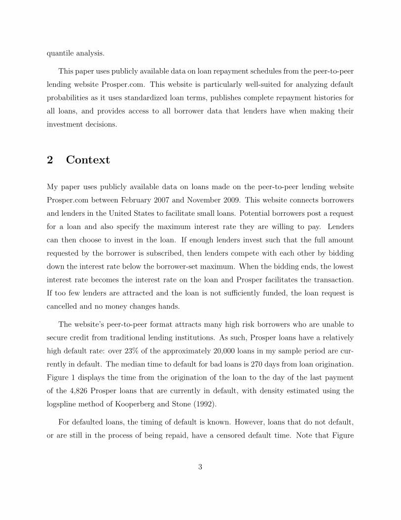
The website’s peer-to-peer format attracts many high risk borrowers who are unable to

secure credit from traditional lending institutions. As such, Prosper loans have a relatively

high default rate: over 23% of the approximately 20,000 loans in my sample period are cur-

rently in default. The median time to default for bad loans is 270 days from loan origination.

Figure 1 displays the time from the origination of the loan to the day of the last payment

of the 4,826 Prosper loans that are currently in default, with density estimated using the

logspline method of Kooperberg and Stone (1992).

For defaulted loans, the timing of default is known. However, loans that do not default,

or are still in the process of being repaid, have a censored default time. Note that Figure

3

1 is limited only to uncensored observations and does not make any attempt to account

for censoring. Thus, we would expect that the true uncensored density of default timing

would put more weight in the right portion of the graph than is observed in the censored

data. Since the sample covers only two and one half years, early defaulters are more likely

to appear as having defaulted than later defaulters.

[Figure 1 about here.]

Prosper provides the data used to generate its website to the public, so that every financial

variable available to the lenders is observed. The borrower financial characteristics considered

in this analysis are the current number of delinquent accounts, the total number of open

credit lines, the number of delinquent accounts in the last seven years, the number of credit

inquiries in the last six months, self-reported employment status, debt to income ratio,

homeownership status, and credit grade, which is derived from the Experion credit rating

and ranges from AA as the most credit-worthy to HR standing for “high risk” as the least

credit-worthy.

Discrete credit grades have been mapped to a credit score derived from the Experion

credit rating range, as described in Table 2. Lenders can also see if borrowers have joined

any Prosper “groups,” voluntary social organizations that do not provide any joint liability.

Other researchers have explored the impact of social organizations on lending terms on

Prosper; see, for example, Freedman and Jin (2008) or Karney and Miller (2009).

Data are available on the amount of the loan and the interest rate of the loan, as well as

the complete repayment history of all loans for all borrowers. All transactions on Prosper

are three-year, uncollateralized loans. Descriptive statistics, as well as a brief description of

each variable, are provided in Table 1.

[Table 1 about here.]

4

3 Cox Proportional Hazard Model

This section uses the proportional hazard model, first proposed by Cox (1974), to analyze

the effect of borrower characteristics on default probability. The model is:

h(t|xi, zi) = h0(t) exp(x>i β + z>i γ). (1)

The Cox model assumes a baseline hazard function, h0(t), that is the same for all borrow-

ers. The model makes no assumptions about the shape of h0(t), but assumes a parametric

form on the effects of observed characteristics. A key assumption is that the effect of the

covariates is multiplicatively seperable from the temporal effect embodied in h0(t), so that

the parameters simply shift the underlying hazard function up or down.

Hazard rates for borrower i at time t are affected by two sets of characteristics: the bor-

rower’s credit-worthiness metrics and the loan terms. Measurements of credit risk included

are credit score, credit score squared, current delinquencies, delinquncies in the last 7 years,

credit inquiries, public records, total number of credit lines, an indicator of living in a city

and full time employment, debt to income ratio, social group membership, and homeown-

ership status. These characteristics are denoted in (1) by xi. The terms of the loan, i.e.

interest rate, interest rate squared, and loan size, are given by zi. Loans that are not in

default are considered to have censored default times.

[Table 2 about here.]

[Table 3 about here.]

[Table 4 about here.]

The Cox estimates are found in Table 3. There are two observations about the estimates

that may be surprising. The first is that having a public record, such as a bankruptcy, has

only a small impact on default probability almost indistinguishable from zero at the 5%

level. This seems implausible, as it implies that past legal entanglements due to poor credit

5

behavior do not have a substantial impact on whether or not a borrower will default on a

new loan. It seems plausible that this finding may reflect institutional constraints and will

be further explored in the quantile regression model in Section 4.

The second observation is that once other financial characteristics are controlled for,

credit score does not measurably impact default probability. Credit score is a function of

both the financial variables included in the model and other financial characteristics that are

not displayed on Prosper. The Cox estimates suggest that the available variables capture

the aspects of credit score that influence default probability and thus the remaining marginal

information contained in credit score is negligible. Even in a model that includes only credit

score and credit score squared, the proportional hazard model does not find individually

significant effects, although a model with only credit score finds a strong negative relationship

between credit score and default probability. See Tables 4 and 5.

Other indicators of credit worthiness appear to consistently predict lower default prob-

abilities in the proportional hazard model. A long credit history is associated with lower

default rates. Borrowers who are employed full time are about 14% less likely to default than

those who are not and those who list a city as their place of residence are about 13% less

likely to default. Having alternative lines of credit also is associated with lower default risk,

as borrowers are able to fall back on other lending sources to make payments. One might

speculate that this type of credit cycling does not work indefinitely. Open credit lines may

also be correlated with family income. Alternatively, credit card companies may have access

to additional credit-worthiness metrics that are not observed on Prosper, and the low default

probability associated with open credit lines may be related to these measures of credit risk.

Current delinquencies and debt to income ratio are associated with higher default risk.

Membership in a Prosper group is also associated with higher credit risk, most likely because

these groups often attract lower quality borrowers; group members default at rates about 12%

higher than non-group members with similar characteristics. See Karney and Miller (2009)

or Freedman and Jin (2008) for more information on Prosper groups. A larger number

of credit inquiries, the number of times banks or businesses request the borrower’s credit

report, is associated with higher default rates, as is home ownership. Credit score, credit

6

score squared and public records are not statistically distinguishable from zero.

Although the Cox model provides a good overview of the effect of borrower characteristic

on default rates, relaxing the assumptions of the model may lead to more nuanced insights.

In the next section, I explore whether the analysis of defaults can be improved using quantile

regression.

4 Censored Quantile Regression Model

The proportionality assumption of the Cox proportional hazard model may be too restrictive

in some cases. Forcing the parameters to shift the baseline hazard up or down monotonically

does not allow the model to identify effects that change over the lifetime of a loan.1 In this

section I briefly summarize the methodology introduced by Portnoy (2003) and describe

results from its application to the model of default timing.

4.1 Methodology

Quantile regression, first introduced by Koenker and Bassett (1978), permits the modeling of

conditional quantiles rather than the conditional mean. In this paper, a quantile regression

treatment of the survival model is useful as it allows the variables to have a different effect

on defaulters based on how long the loan has been active.

In other quantile duration studies, such as those by Koenker and Geling (2001) and

Koenker and Bilias (2001), random censoring is not an issue: the “event time” is known

1The validity of this assumption has been explored in other duration applications. For

example, in a study of the mortality of fruitflies, Koenker and Geling (2001) find that at high

survival times, the effect of gender reverses: early in their lives, male fruitflies have better

survival rates than females, but if they make it to a sufficiently advanced age, the gender

effect reverses sign and female flies have better survival prospects. These crossover effects

are not possible to capture in a traditional Cox proportional hazard model.

7

for all observations. However, in the Prosper data, all loans that are not in default are

considered censored. As only about 20% of the loans are in default, censoring is present in

a significant degree.

The problem of estimating the conditional quantile functions when the data are censored

was first explored by Powell (1984). Consider the case of right-censored data where the event

time Yi is observed if Yi < Ci, where Ci indicates a censoring time. In our application, Yi is

the time of default, measured in days, since the origination of the loan, and we use log(Yi)

as our right-hand side variable.

Event times are a function of covariates xi ∈ Rj, so that the observed Yi = min{Ci, x>i β+

ui} and the data set consists of a vector of pairs (Yi, xi). In a situation where the censoring

times Ci are known for all observations (i.e., “fixed censoring”), Powell (1986) shows that the

conditional quantile function for each quantile τ can be consistently estimated by solving,

β = arg minβ∈Rp

N∑i=1

ρτ (Yi −max(Ci, x′iβ)) (2)

where ρτ (u) = u(τ − I(u < 0)) and I(.) is the indicator function.

Unfortunately, censoring times Ci are not always known for all observations. With ran-

dom censoring, the censoring times are only observed for the observations that are censored.

To further complicate matters, the probability of being censored may depend on the covari-

ates themselves. In our case, the probability of being censored–that is, of not defaulting–is

positively correlated with a borrower’s credit-worthiness.

Kaplan and Meier (1958) introduced a non-parametric approach to analyzing survival

data with random censoring. They propose estimating the probability of surviving time t by

dividing the difference of nt, the number of observations neither dead nor censored at time

t (i.e., those “at risk”), and the number of observations “dead” at time t, dt, by nt. Then,

the probability of surviving beyond time t is the product of the conditional probabilities of

surviving all previous periods and t, 1, 2, ..., t−1, t. The probability of surviving passed time

t, denoted S(t), is

S(t) = P (Yi > t) = 1− F (Yi), (3)

8

and its estimate is given as

S(t) =∏ti≤t

pi =∏ti≤t

ni − dini

. (4)

Efron (1967) noted that the Kaplan Meier estimator is essentially a reweighting scheme

that moves some of the weight of the censored observations to pseudo-observations at points

above the observed Yi; for example, positive infinity.

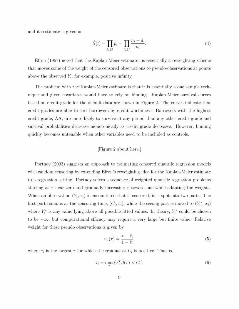
The problem with the Kaplan-Meier estimate is that it is essentially a one sample tech-

nique and given covariates would have to rely on binning. Kaplan-Meier survival curves

based on credit grade for the default data are shown in Figure 2. The curves indicate that

credit grades are able to sort borrowers by credit worthiness. Borrowers with the highest

credit grade, AA, are more likely to survive at any period than any other credit grade and

survival probabilities decrease monotonically as credit grade decreases. However, binning

quickly becomes untenable when other variables need to be included as controls.

[Figure 2 about here.]

Portnoy (2003) suggests an approach to estimating censored quantile regression models

with random censoring by extending Efron’s reweighting idea for the Kaplan-Meier estimate

to a regression setting. Portnoy solves a sequence of weighted quantile regression problems

starting at τ near zero and gradually increasing τ toward one while adapting the weights.

When an observation (Yi, xi) is encountered that is censored, it is split into two parts. The

first part remains at the censoring time, (Ci, xi), while the secong part is moved to (Y ∗i , xi)

where Y ∗i is any value lying above all possible fitted values. In theory, Y ∗i could be chosen

to be +∞, but computational efficacy may require a very large but finite value. Relative

weight for these pseudo observations is given by

wi(τ) =τ − τi1− τi

. (5)

where τi is the largest τ for which the residual at Ci is positive. That is,

τi = maxτ{xTi β(τ) < Ci} (6)

9

The following estimate of the coefficients β(τ) for each quantile τ are chosen to solve the

minimization problem

minβ∈Rp

∑i/∈K

ρτ (Yi − x>i β) +∑i∈K

wi(τ)ρτ (Ci − x>i β) + (1− wi(τ))ρτ (Y∗ − x>i β), (7)

where K denotes the set of censored observations that have been encountered up to quantile

τ .

In a one-sample setting, this estimation method will produce the same quantile function

as the Kaplan Meier technique; i.e. the quantile function corresponding to F (t) = 1− S(t).

4.2 Results

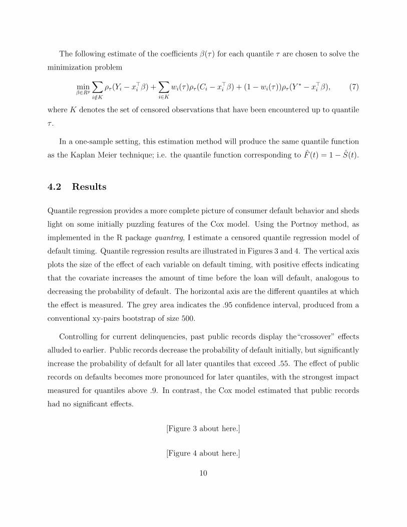
Quantile regression provides a more complete picture of consumer default behavior and sheds

light on some initially puzzling features of the Cox model. Using the Portnoy method, as

implemented in the R package quantreg, I estimate a censored quantile regression model of

default timing. Quantile regression results are illustrated in Figures 3 and 4. The vertical axis

plots the size of the effect of each variable on default timing, with positive effects indicating

that the covariate increases the amount of time before the loan will default, analogous to

decreasing the probability of default. The horizontal axis are the different quantiles at which

the effect is measured. The grey area indicates the .95 confidence interval, produced from a

conventional xy-pairs bootstrap of size 500.

Controlling for current delinquencies, past public records display the“crossover” effects

alluded to earlier. Public records decrease the probability of default initially, but significantly

increase the probability of default for all later quantiles that exceed .55. The effect of public

records on defaults becomes more pronounced for later quantiles, with the strongest impact

measured for quantiles above .9. In contrast, the Cox model estimated that public records

had no significant effects.

[Figure 3 about here.]

[Figure 4 about here.]

10

These results are consistent with the initial premise that the structure of U.S. bankruptcy

law effects the impact of past bankruptcies on current default probability differently over

time: after declaring bankruptcy, a debtor cannot file for bankruptcy again for four years.

Since these are three year loans, these prohibitions sometimes expire over the course of a

loan’s lifetime. The quantile model suggests that borrowers with past bankruptcies or liens

are not equally risky as those borrowers without such a history, as a naive researcher might

conclude from the Cox model, but rather that they are less credit-worthy borrowers who

are temporarily facing an institutional constraint. These results may explain, in part, why

post-bankruptcy borrowers are often aggressively solicited by lenders (see, e.g., Cohen-Cole

et al. (2009)).

The traditional credit risk summary measure, credit score, also invites a slightly different

interpretation when estimated using quantile regression. Whereas the Cox model estimated

the marginal impact of credit score and credit score squared to be indistinguishable from

zero once other observed credit metrics are controlled for, the quantile model finds significant

effects for the middle of the distribution (between τ = .3 and τ = .6). Although the

additional information contained in credit score may not be useful for very early or very late

defaulters, it helps predict default for intermediate durations and should not be discarded.

The Portnoy estimator provides a more nuanced interpretation of the effect of “open

credit lines.” Open credit lines are associated with higher repayment rates early in the loan’s

life, presumably because in hard times a borrower can fall back on other credit sources to

make loan payments. However, this credit cycling behavior does not last forever and the

effect eventually fades. For late defaulters, more credit lines do not decrease default prob-

ability, and the estimates of the effect for higher quantiles are negative, albeit statistically

insignficant. This crossover conjures the image of a frazzled borrower paying credit card bills

off with other credit cards – the strategy works for a while, but eventually the debt becomes

overwhelming.

The usefulness of other measures of credit worthiness in predicting defaut behavior also

change over time. For example, homeownership has little effect on upper and lower quantiles,

but significantly increases default probability for middle quantiles. Membership in a Prosper

11

social group prevents early default, but it is associated with higher default for most quantiles.

Groups may attract high credit risks that represent a poor investment overall, but they do

decrease the risk of potentially embarassing very early defaults, possibly through social

pressure.

To facilitate interpretation of the quantile regression results, the cumulative probability of

default is plotted against time in Figure 5. Distinct quantiles are smoothed for presentation

using a “running median” smoother (see Tukey (1977)). The y-axis indicates probability

of defaulting at or before a certain time. The x-axis plots time, by day, from the origin of

the loan. The lines indicates the cumulative predicted default probability for a borrower

with no public records (solid) and a borrower with four public records (dashed). All other

characteristics are evaluated at the sample median. In the first year of the loan, a borrower

with public records is less likely to default than a borrower without public records. The

last two years of the loan, the order switches, and the borrower with public records is more

likely to default. These differences are plotted by month in 6. Although these differences are

relatively modest, considering the volume of loans on Prosper alone exceeds $130 million, a

one to two percent change in the probability of default represents a substantial monetary

value. Additionally, the timing of default alters the recovery rates on defaulted loans in a

way that is potentially relevant to investor profit calculations.

[Figure 5 about here.]

[Figure 6 about here.]

5 Conclusion

This paper provides analyzes default behavior in loan performance data using the Cox pro-

portional hazard model and censored quantile regression. Using the (censored) repayment

histories of over 20,000 loans from Prosper.com, I find evidence that some traditional pre-

dictors of default behave differently for early or late defaulters, including “crossover” effects

that cannot be captured by a Cox proportional hazard model.

12

References

Adams, W., L. Einav, and J. Levin (2009). Liquidity constraints and imperfect information

in subprime lending. The American Economic Review 99 (1), 49–84.

Cohen-Cole, E., B. Duygan-Bump, and J. Montoriol-Garriga (2009). Forgive and forget:

Who gets credit after bankruptcy and why? Working Paper Series: Federal Reserve Bank

of Boston.

Cox, D. (1974). Regression models with life tables. Journal of the Royal Statistical Society 34,

187–220.

Efron, B. (1967). The two-sample problem with censored data. Proc. Fifth Berkeley Sym-

posium in Mathematical Statistics 4.

Freedman, S. and G. Jin (2008). Do social networks solve information problems for peer-to-

peer lending? Evidence from Prosper.com. Working Paper.

Kaplan, E. and P. Meier (1958). Nonparametric estimation from incomplete observations.

Journal of the American Statistical Association 53, 457–481.

Karney, D. and S. Miller (2009). Social lending and microcredit: Evidence from Prosper.com.

Working Paper.

Koenker, R. and G. W. Bassett (1978). Regression quantiles. Econometrica 46 (1), 33–50.

Koenker, R. and Y. Bilias (2001). Quantile regression for duration data: A reappraisal of

the Pennsylvania re-employment bonus experiments. Empirical Economics 26, 199–200.

Koenker, R. and O. Geling (2001). Reappraising medfly longevity: A quantile regression

survival analysis. Journal of the American Statistical Association 96, 458–468.

Kooperberg, C. and C. J. Stone (1992). Logspline density estimation for censored data.

Journal of Computational and Graphical Statistics 1, 301–328.

Portnoy, S. (2003). Censored regression quantiles. Journal of the American Statistical As-

sociation 98 (464), 1001–1012.

13

Powell, J. (1984). Least absolute deviations estimation for the censored regression model.

Journal of Econometrics 25, 303–325.

Powell, J. (1986). Censored regression quantiles. Journal of Econometrics 32, 143–155.

Ravina, E. (2008). Love and loans: The effect of beauty and personal characteristics in credit

markets. Working Paper.

Tukey, J. (1977). Exploratory Data Analysis. Reading, Massachusetts: Addison-Wesley.

14

Tab

le1:

Des

crip

tive

Sta

tist

ics

Var

iable

Nam

eD

escr

ipti

onM

ean

Min

/Max

Am

ount

Dol

lar

amou

nt

oflo

an65

3610

00/2

5000

Bor

row

erR

ate

Inte

rest

rate

pai

dby

bor

row

er18.0

30.

01/3

6.00

Cit

yD

um

my

Bin

ary

vari

able

takin

ga

valu

eof

1if

the

bor

row

er0.

160/

1

isa

resi

den

tof

aci

ty

Curr

entD

elin

quen

cies

Num

ber

ofcr

edit

lines

curr

entl

y1.

020/

83

list

edas

del

inquen

t

Deb

tToI

nco

meR

atio

Rat

ioof

dol

lar

valu

eof

outs

tandin

gdeb

t.3

40/

10

tose

lf-r

epor

ted

inco

me

Del

inquen

cies

Las

t7Y

ears

Num

ber

ofdel

inquen

tac

counts

inth

ela

stse

ven

year

s5.

130/

99

Fullti

me

Bin

ary

vari

able

takin

ga

valu

eof

1if

the

bor

row

er0.

880/

1

rep

orts

they

are

afu

ll-t

ime

emplo

yee

Gro

upD

um

my

Bin

ary

vari

able

takin

ga

valu

eof

1if

the

0.31

0/1

bor

row

eris

am

emb

erof

aP

rosp

erso

cial

grou

p

Hom

eB

inar

yva

riab

leta

kin

ga

valu

eof

1if

the

bor

row

er0/

1

isa

hom

eow

ner

Inquir

iesL

ast6

Mon

ths

Num

ber

ofti

mes

the

cred

itre

por

thas

bee

n2.

650/

63

PublicR

ecor

dsL

ast1

0Yea

rsN

um

ber

ofpublic

reco

rds,

such

asban

kru

ptc

ies

orlien

s,0.

380/

30

list

edon

the

bor

row

er’s

cred

itre

por

t.

Op

enC

redit

Lin

esN

um

ber

ofac

tive

lines

ofcr

edit

inth

eb

orro

wer

’snam

e8.

210/

45

15

Table 2: Credit Grade-Category Mapping

Grade Credit Score Range Credit Score Assigned Percent of SampleAA 760− 850 805.5 12.86A 720− 759 739.5 12.57B 680− 719 699.5 16.59C 640− 679 659.5 21.78D 600− 639 619.5 19.07E 560− 599 579.5 8.88

HR 520− 559 539.5 9.08

16

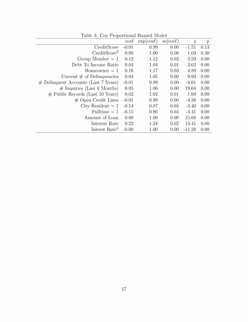
Table 3: Cox Proportional Hazard Modelcoef exp(coef) se(coef) z p

CreditScore -0.01 0.99 0.00 -1.51 0.13CreditScore2 0.00 1.00 0.00 1.03 0.30

Group Member = 1 0.12 1.12 0.03 3.59 0.00Debt To Income Ratio 0.04 1.04 0.01 3.62 0.00

Homeowner = 1 0.16 1.17 0.03 4.89 0.00Current # of Delinquencies 0.04 1.05 0.00 9.93 0.00

# Delinquent Accounts (Last 7 Years) -0.01 0.99 0.00 -4.61 0.00# Inquiries (Last 6 Months) 0.05 1.06 0.00 19.64 0.00

# Public Records (Last 10 Years) 0.02 1.02 0.01 1.69 0.09# Open Credit Lines -0.01 0.99 0.00 -4.38 0.00

City Resident = 1 -0.14 0.87 0.04 -3.40 0.00Fulltime = 1 -0.15 0.86 0.04 -3.41 0.00

Amount of Loan 0.00 1.00 0.00 15.68 0.00Interest Rate 0.22 1.24 0.02 14.41 0.00Interst Rate2 -0.00 1.00 0.00 -11.28 0.00

17

Table 4: Cox Proportional Hazard Model: Credit Score and Credit Score Squaredcoef exp(coef) se(coef) z p

Credit Score -0.00 1.00 0.00 -1.17 0.24Credit Score2 -0.00 1.00 0.00 -0.58 0.56

18

Table 5: Cox Proportional Hazard Model: Credit Scorecoef exp(coef) se(coef) z p

Credit Score -0.01 0.99 0.00 -26.56 0.00

19

Figure 1: Days from Origin of Loan to Default for Defaulted Loans, Logspline DensityEstimation

0 200 400 600 800

0.00

000.

0010

0.00

20

Days Until Default

Den

sity

20

0 200 400 600 800 1000

0.4

0.5

0.6

0.7

0.8

0.9

1.0

Days from Origination

Pro

babi

lity

of S

urvi

val

Figure 2: Kaplan-Meier Survival Curves by Credit GradeBlack indicates highest credit rating, AA. Increasingly lighter greys indicate A, B, C, D, E, and

HR ratings respectively.

21

Figure 3: Conditional Quantile Effects on Time to Default - 1

0.2 0.4 0.6 0.8

−0.

020.

040.

08

CreditScore

o o o o o o o oo

oo o o

oo

o

oo

0.2 0.4 0.6 0.8

−8e

−05

−2e

−05

CreditScore2

o o o o o o o oo

oo o o

o oo

o o

0.2 0.4 0.6 0.8

−1.

00.

00.

5

GroupDummy

oo o o

oo o o o o

o oo o

oo

o o

0.2 0.4 0.6 0.8−0.

0001

2−

0.00

004

Amount

o oo

oo

o o oo o

oo o o o

o

o o

0.2 0.4 0.6 0.8

−2.

0−

1.0

0.0

BorrowerRate

o o o o o o o o o o o o o

o o o

oo

0.2 0.4 0.6 0.8

0.00

0.02

0.04

BorrowerRate2

o o o o o o o o o o o o o

o o o

oo

0.2 0.4 0.6 0.8

−0.

15−

0.05

DebtToIncomeRatio

oo

oo

oo

oo o o

o o oo

o

o o o

0.2 0.4 0.6 0.8

−0.

60.

00.

4

Home

oo o o o

o o o o oo

oo o

o

o

o o

0.2 0.4 0.6 0.8

−0.

100.

00

CurrentDelinquencies

oo o o o o o o o o

o o o oo

oo o

22

Figure 4: Conditional Quantile Effects on Time to Default - 2

0.2 0.4 0.6 0.8

−0.

020.

000.

02

DelinquenciesLast7Years

o oo o o o o

o o o o oo

oo

o

o o

0.2 0.4 0.6 0.8

−0.

12−

0.06

InquiriesLast6Months

o oo o o o o o

oo

o o o o oo

o o

0.2 0.4 0.6 0.8

−0.

150.

00

PublicRecordsLast10Years

o

oo

o o o o o oo

oo o o

oo o o

0.2 0.4 0.6 0.8

−0.

100.

00

OpenCreditLines

o o o o o o o o o o o o o o

oo

o o

0.2 0.4 0.6 0.8

−0.

40.

20.

61.

0

CityDummy

o o o oo o o o

oo o

o o

oo

o

o o

0.2 0.4 0.6 0.8−

0.5

0.5

Fulltime

o o o o o o o o o o o oo

o o

o

oo

23

Figure 5: Conditional Quantile Effects of Public Records on Time to Default0 Public Records (Solid) vs. 4 Public Records (Dashed)

Days Until Default

Cum

ulat

ive

Pro

babi

lity

of D

efau

lt

0.00

0.05

0.10

0.15

0.20

0.25

0 200 400 600 800 1000

24

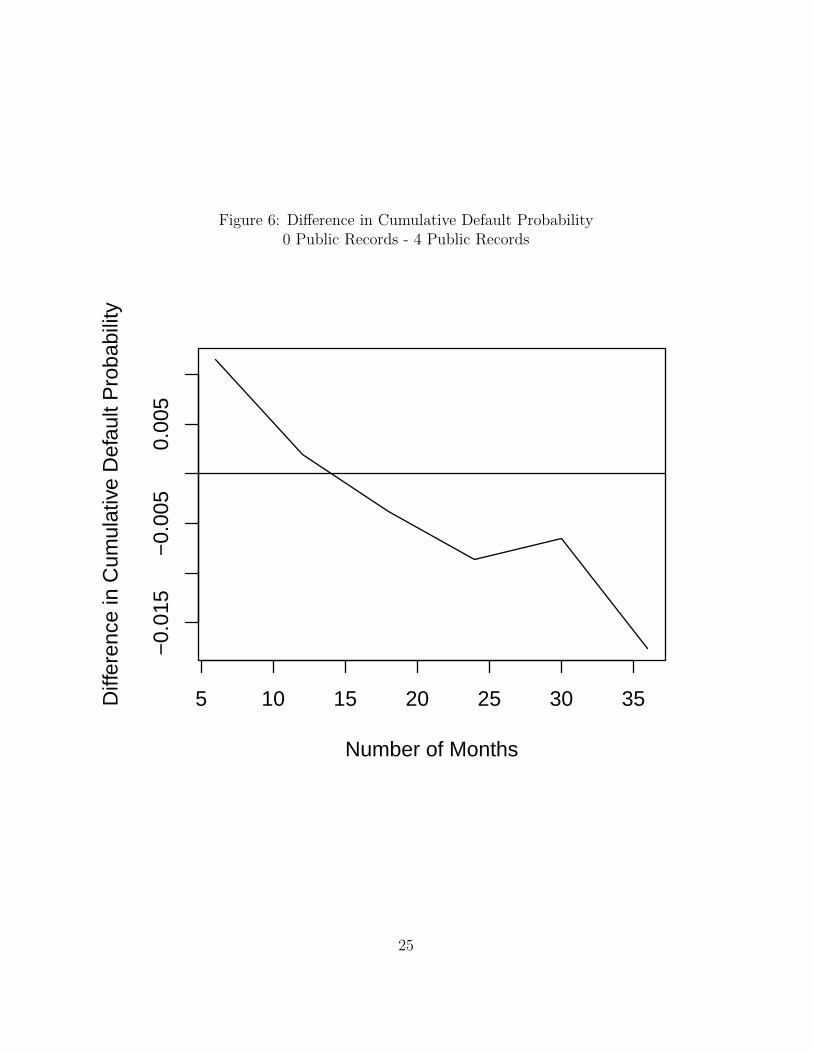
Figure 6: Difference in Cumulative Default Probability0 Public Records - 4 Public Records

5 10 15 20 25 30 35

−0.

015

−0.

005

0.00

5

Number of Months

Diff

eren

ce in

Cum

ulat

ive

Def

ault

Pro

babi

lity

25